A Stochastic Alternating Direction Method of Multipliers for Non-smooth and Non-convex Optimization

Abstract

Alternating direction method of multipliers (ADMM) is a popular first-order method owing to its simplicity and efficiency. However, similar to other proximal splitting methods, the performance of ADMM degrades significantly when the scale of the optimization problems to solve becomes large. In this paper, we consider combining ADMM with a class of stochastic gradient with variance reduction for solving large-scale non-convex and non-smooth optimization problems. Global convergence of the generated sequence is established under the extra additional assumption that the object function satisfies Kurdyka-Łojasiewicz (KL) property. Numerical experiments on graph-guided fused Lasso and computed tomography are presented to demonstrate the performance of the proposed methods.

Key words. Non-convex optimization $\cdot$ stochastic ADMM $\cdot$ variance reduction stochastic gradient

AMS subject classifications. 90C26 $\cdot$ 90C30 $\cdot$ 90C90 $\cdot$ 15A83 $\cdot$ 65K05

1 Introduction

Driven by the problems arising from diverse fields including signal/image processing, compressed sensing, inverse problems, computer vision and many others, the past decades have witnessed a tremendous success of non-smooth optimization and first-order proximal splitting algorithms [7]. Nowadays, with the advances of data acquisition tools and mathematical modeling, the problems to handle are becoming increasingly complex which imposes challenges, e.g. large dimension and non-smoothness, to design efficient numerical algorithms. In the fields of machine learning and related areas, stochastic optimization methods are widely adopted due its simplicity and fast convergence. Over the past few years, in traditional areas such as imaging science, stochastic methods are becoming popular due to the aforementioned challenges. In this paper, we follow this path and consider a stochastic version of the popular alternating direction method of multipliers (ADMM) [11, 35].

In this paper, we are interested in solving the following composite optimization problem

$$\min_{x\in\mathbb{R}^{d}}H(x)+F(Ax),$$ (1.1)

where $H=\frac{1}{n}\sum_{i=1}^{n}H_{i}(x)$ has finite sum structure, $A:\mathbb{R}^{d}\to\mathbb{R}^{m}$ is a linear mapping and $H,F$ are proper lower semi-continuous functions. Throughout this paper, no convexity is imposed to either $H$ or $F$. In practice, numerous problems can be formulated in to the form of (1.1). For example, in computed tomography (CT), the reconstruction task can be modeled as

$$\min_{x\in\mathbb{R}^{d}}{{\frac{\raisebox{0.41669pt}{\footnotesize$1$}}{\raisebox{-1.24994pt}{\footnotesize$n$}}}}\sum_{i=1}^{n}(\mathcal{R}_{i}x-b_{i})^{2}+F(Ax),$$ (1.2)

where $x$ is the image to be reconstructed, $n$ is the number of projection, $\mathcal{R}$ is Radon transform, $b_{i}$ is the $i_{th}$ observation. In order to ensure the quality of the reconstructed image, a large amount of projection is required, which means a large value of $n$. Another example is classification/regression, where one needs to solve the following problem

$$\min_{x\in\mathbb{R}^{d}}{{\frac{\raisebox{0.41669pt}{\footnotesize$1$}}{\raisebox{-1.24994pt}{\footnotesize$n$}}}}\sum_{i=1}^{n}H(a_{i}^{T}x,y_{i})+F(Ax),$$

where for each $i=1,...,n$, $(a_{i},y_{i})\in\mathbb{R}^{n}\times\mathbb{R}$ is given training data and its corresponding label; $H$ is the loss function, such as square loss or logistic loss. In many cases, one needs to use a large scale of training data which results in huge value of $n$. In both cases, $F(Ax)$ is called regularization term, where $A$ is a properly chosen linear transformation such as discrete gradient operator or wavelet transform, and $F$ is a low-complexity promoting functions such as $L_{0}$ or $L_{1}$-norms for sparsity. We refer to [46, 52, 45, 2, 43] and the references therein for more detailed discussions.

1.1 Alternating direction method of multipliers

In the literature, one popular method to solve (1.1) is alternating direction method of multipliers (ADMM). ADMM was developed around 1970s, where [11, 35] shaped the original form of the algorithm, deeper theoretical understanding of ADMM can be found in [12] and the nowadays popularity of ADMM partially owes to [6]. To apply ADMM to solve (1.1), one needs to add an auxiliary variable $z$ which leads to the following constrained problem

$$\min_{x\in\mathbb{R}^{d},u\in\mathbb{R}^{m}}H(x)+F(z)\quad\textrm{such\,that}\quad z=Ax.$$ (1.3)

The augmented Lagrangian formulation associated to (1.3) reads

$$\mathcal{L}_{\beta}(x,z,u)=F(z)+H(x)+\langle u,Ax-z\rangle+{{\frac{\raisebox{0.41669pt}{\footnotesize$\beta$}}{\raisebox{-1.24994pt}{\footnotesize$2$}}}}\|Ax-z\|^{2},$$

where $u$ is the Lagrange multiplier and $\beta>0$ is properly chosen [11, 35]. In this paper, we adopt a linearized ADMM proposed in [29, 47, 50, 36, 34], which takes the following form of iteration

$$z_{t+1} \in\arg\min_{z}F(z)+\langle u_{t},Ax_{t}-z\rangle+{{\frac{\raisebox{0.41669pt}{\footnotesize$\beta$}}{\raisebox{-1.24994pt}{\footnotesize$2$}}}}\|Ax_{t}-z\|^{2},$$ (1.4)

$$x_{t+1} =x_{t}-{{\frac{\raisebox{0.41669pt}{\footnotesize$1$}}{\raisebox{-1.24994pt}{\footnotesize$\tau$}}}}\big{(}{\nabla H(x_{t})+A^{T}u_{t}+\beta A^{T}(Ax_{t}-z_{t+1})}\big{)},$$

$$u_{t+1} =u_{t}+\sigma\beta(Ax_{t+1}-z_{t+1}),$$

where $\tau,\sigma>0$ are step-sizes. The difference between (1.4) and the standard ADMM lies in the update of $x_{t+1}$, for standard ADMM one needs to solve a proximal minimization of $H(x)$, while (1.4) takes the gradient descent for $H$.

Convergence guarantees of (1.4) in the convex case can be found in [29, 47, 50], while for the non-convex case results are available in [36, 34]. For the case of $H$ being a finite sum, computing the full gradient $\nabla H$ can be very time consuming which damps the efficiency of the method. To circumvent such difficulty, one can replace $\nabla H$ with its stochastic approximation, which results in a stochastic version of (1.4) and is the core of our contributions in this work.

1.2 Contributions

Motivated by the work of [10], in this paper we propose a stochastic version of ADMM (1.4) for solving non-smooth and non-convex objective (1.1). The key of our algorithm is replacing the full gradient computation $\nabla H$ in (1.4) with its stochastic approximations $\widetilde{\nabla}H$, and the resulted algorithm is described below in Algorithm 1.

  Step 0. Input $T$ and $\beta,\,\tau,\,\sigma>0$. Initialize $x_{0}$ and $u_{0}$.

  Step 1. For $t=0,1,\dots,T-1$ do

$$z_{t+1} \in\arg\min_{z}F(z)+\langle u_{t},Ax_{t}-z\rangle+{{\frac{\raisebox{0.41669pt}{\footnotesize$\beta$}}{\raisebox{-1.24994pt}{\footnotesize$2$}}}}\|Ax_{t}-z\|^{2},$$ (1.5a)

$$x_{t+1} =x_{t}-{{\frac{\raisebox{0.41669pt}{\footnotesize$1$}}{\raisebox{-1.24994pt}{\footnotesize$\tau$}}}}\big{(}{\widetilde{\nabla}H(x_{t})+A^{T}u_{t}+\beta A^{T}(Ax_{t}-z_{t+1})}\big{)},$$ (1.5b)

$$u_{t+1} =u_{t}+\sigma\beta(Ax_{t+1}-z_{t+1}).$$ (1.5c)

  Step 2. Iterate $x$ and $z$ chosen uniformly random from $\{x_{t},z_{t}\}_{t=1}^{T}$.

Algorithm 1 A Stochastic Alternating Direction Method of Multipliers (SADMM)

Various stochastic gradient approximations developed in the literature can be used by $\widetilde{\nabla}H$, for instance the simplest choice is the stochastic gradient [22]. Since $H$ has finite sum structure, variance reduced stochastic gradient approximations can also be applied, such as SAGA [3] and SVRG [38] which are unbiased, and SARAH [30] which is biased. Overall, our contributions in this paper consist the following

• By combing ADMM with stochastic gradient approximations, we propose a stochastic ADMM algorithm for non-convex and non-smooth optimization. Our algorithm is very general in the sense that it can incorporate with most existing stochastic gradient approximation in the literature.

• When the stochastic gradient approximation $\widetilde{\nabla}H$ is variance reduced (see Definition 2.1), a decent property is obtained for a specifically designed stability function which yields the convergence of the objective function. If moreover the objective function has Kurdyka-Łojasiewicz property (see Definition 2.6), convergence of the generated sequences is also established.

• Numerically, we test performance of SADMM using several well studied stochastic gradient approximations (e.g. SGD, SAGA, SVRG and SARAH) on problems including graph-guided fused Lasso, wavelet frame based 2D CT reconstruction and TV-L0 3D CT reconstruction. We also compare with some existing algorithms in the literature, and our result indicates SADMM achieves the best performance using SARAH gradient approximation.

1.3 Related work

Over the past years, extension of ADMM to the case of non-convex optimization and stochastic setting are widely studied. Along the direction of non-convex optimization, recently some theoretical foundations are established. For instance in [17], the authors studied the convergence of ADMM for a class of non-convex optimization problems. In [16, 15], convergence of a non-convex Bregman ADMM was studied. For non-convex separable objective functions with applications to consensus problem, the authors of [32] studied the properties of ADMM. Other related work can be found in for instance [51, 37] under different settings. It should be noted that all these works are studied under the deterministic setting, that is no randomness is involved in these results.

For stochastic versions of ADMM, the first attempt can be found in [23], where the authors proposed an online ADMM for large scale optimization. In recent years, the success of stochastic proximal gradient algorithms, such as SAG/SAGA [33, 4], SDCA [40], SVRG [38, 28] and SARAH [30], greatly boost the studies of stochastic ADMM. For example, in [31] the authors combined ADMM with SAG gradient approximation, which was further combined with Nesterov acceleration [49] in [39]. Stochastic ADMM with SDCA was studied in [44] for a wide range of regularized learning problems, and linear rate of convergence was obtained when the objective function obeys some strong convexity and smoothness property. The combinations of ADMM with SVRG can be found in [42, 48] under different settings. We also refer to [41] for related developments of stochastic ADMM. In [13] the authors studied the combination of ADMM and three different gradient approximations: SGD, SVRG and SAGA, for solving non-convex non-smooth problems. For each gradient approximation, the authors proved that $(x_{t^{*}},z_{t^{*}})$ is an $\varepsilon$-stationary point of the objective function, where $t^{*}=\arg\min_{2\leq t\leq T+1}\theta_{t}$ with $\theta_{t}$ being a variable associated the gradient estimator, while the authors showed that the mini-batch SGD/SVRG/SAGA-ADMM has a convergence rate of $\mathcal{O}({{\frac{\raisebox{0.29167pt}{\footnotesize$1$}}{\raisebox{-0.87495pt}{\footnotesize$T$}}}})$. Similar approach is used in [14] for the convergence analysis of a faster non-convex stochastic ADMM, which using a stochastic path-integrated differential estimator.

In comparison, our work is motivated by [10] where the authors proposed a generic stochastic version proximal alternating linearized minimization (PALM) algorithm [26], for which various variance-reduced gradient approximations are allowed. We extend the result of [10] to the case of ADMM, hence our proposed SADMM is very general in the sense that Algorithm 1 works with any stochastic gradient approximations which are variance reduced.

Paper organisation

The rest of the paper is organized as following. In Section 2, we collect some useful preliminary results which are essential to our analysis. The main theoretical analysis of our proposed algorithm can be found in Section 3, followed by numerical result in Section 4. Proofs of main theorems are differed in the appendix.

2 Preliminaries

In this section, we give some notation and definitions used in our paper. For theoretical analysis, we first recall the definition of variance reduction gradient estimators which is taken from [10].

Definition 2.1 ([10, Definition 2.1]).

A gradient estimator $\widetilde{\nabla}$ is called variance-reduced if there exist constants $V_{1},\,V_{2},\,V_{\Upsilon}\geq 0$ and $\rho\in(0,1]$ such that

• $($MSE Bound$)$ There exists a sequence having random variables $\{\Upsilon_{t}\}_{t\geq 1}$ of the form $\Upsilon_{t}=\sum_{i=1}^{s}\|v_{t}^{i}\|^{2}$ for some random vectors $v_{t}^{i}$ such that

  $$\mathbb{E}_{t}\|\widetilde{\nabla}H(x_{t})-\nabla H(x_{t})\|^{2}\leq\Upsilon_{t}+V_{1}(\mathbb{E}_{t}\|x_{t+1}-x_{t}\|^{2}+\|x_{t}-x_{t-1}\|^{2}),$$

  and, with $\Gamma_{t}=\sum_{i=1}^{s}\|v_{t}^{i}\|,$

  $$\mathbb{E}_{t}\|\widetilde{\nabla}H(x_{t})-\nabla H(x_{t})\|\leq\Gamma_{t}+V_{2}(\mathbb{E}_{t}\|x_{t+1}-x_{t}\|+\|x_{t}-x_{t-1}\|).$$ (2.1)

• $($Geometric Decay$)$ The sequence $\{\Upsilon_{t}\}_{t\geq 1}$ decays geometrically:

  $$\mathbb{E}_{t}\Upsilon_{t+1}\leq(1-\rho)\Upsilon_{t}+V_{\Upsilon}\big{(}{\mathbb{E}_{t}\|x_{t+1}-x_{t}\|^{2}+\|x_{t}-x_{t-1}\|^{2}}\big{)}.$$ (2.2)

• $($Convergence of Estimator$)$ For all sequences $\{x_{t}\}_{t=0}^{\infty}$ satisfying $\lim_{t\to\infty}\mathbb{E}\|x_{t}-x_{t-1}\|^{2}$ $\to 0,$ it follows that $\mathbb{E}\Upsilon_{t}\to 0$ and $\mathbb{E}\Gamma_{t}\to 0$.

As remarked in [10], most existing variance reduced gradient estimators in the literature satisfy the above definition, in this work we mainly consider SAGA [3] and SARAH [30] which are widely used. For these two estimators, we provide their definitions below and refer to Appendix A for their properties.

Definition 2.2 (SAGA [3]).

The SAGA gradient approximation $\widetilde{\nabla}^{\textnormal{\tiny SAGA}}H(x)$ is defined as follows:

$$\widetilde{\nabla}^{\textnormal{\tiny SAGA}}H(x_{t})={{\frac{\raisebox{0.41669pt}{\footnotesize$1$}}{\raisebox{-1.24994pt}{\footnotesize$b$}}}}{\big{(}}{\sum\nolimits_{j\in J_{t}}\nabla H_{j}(x_{t})-\nabla H_{j}(\varphi_{t}^{j})}{\big{)}}+{{\frac{\raisebox{0.60004pt}{\footnotesize$1$}}{\raisebox{-1.79993pt}{\footnotesize$n$}}}}\sum\nolimits_{i=1}^{n}\nabla H_{i}(\varphi_{t}^{i}),$$

where $J_{t}$ is mini-batches containing $b$ indices. The variables $\varphi_{t}^{i}$ follow the update rules $\varphi_{t+1}^{i}=x_{t}$ if $i\in J_{t}$ and $\varphi_{t+1}^{i}=\varphi_{t}^{i}$ otherwise.

Definition 2.3 (SARAH [30]).

The SARAH estimator reads for $t=0$ as

$$\widetilde{\nabla}^{\textnormal{\tiny SARAH}}H(x_{0})=\nabla H(x_{0}).$$

For $t=1,2,\dots$, define random variables $p_{t}\in\{0,1\}$ with $P(p_{t}=0)=\frac{1}{p}$ and $P(p_{t}=1)=1-\frac{1}{p}$, where $p\in(0,\infty)$ is a fixed chosen parameter. Let $J_{t}$ be a random subset uniformly drawn from $\{1,\dots,n\}$ of fixed batch size $b$. Then for $t=1,2,\dots$ the SARAH gradient approximation reads as

$$\widetilde{\nabla}^{\textnormal{\tiny SARAH}}H(x_{t})=\left\{\begin{aligned} \nabla H(x_{t})&:\textrm{if}\,p_{t}=0,\\ {{\frac{\raisebox{0.41669pt}{\footnotesize$1$}}{\raisebox{-1.24994pt}{\footnotesize$b$}}}}\big{(}{\mathbin{\scalebox{0.9}{$\sum$}}_{j\in J_{t}}\nabla H_{j}(x_{t})-\nabla H_{j}(x_{t-1})}\big{)}+\widetilde{\nabla}^{\textnormal{\tiny SARAH}}H(x_{t-1})&:\textrm{if}\,p_{t}=1.\end{aligned}\right.$$

Below we include supermartingale convergence result, and refer to [9] and [21] for more details.

Lemma 2.4.

Suppose $x_{1},\dots,x_{t}$ are independent random variables satisfying $\mathbb{E}_{t}x_{i}=0$ for all $i$. Then

$$\mathbb{E}_{t}\|x_{1}+\cdots+x_{t}\|^{2}=\mathbb{E}_{t}\big{[}\|x_{1}\|^{2}+\cdots+\|x_{t}\|^{2}\big{]}.$$

Lemma 2.5 (Supermartingale Convergence Theorem).

Let $\mathbb{E}_{t}$ denote the expectation conditional on the first $t$ iterations of Algorithm 1. Let $\{X_{t}\}_{t=0}^{\infty}$ and $\{Y_{t}\}_{t=0}^{\infty}$ be sequences of bounded non-negative random variables such that $X_{t}$ and $Y_{t}$ depend only on the first $t$ iterations of Algorithm 1. If

$$\mathbb{E}_{t}X_{t+1}+Y_{t}\leq X_{t},$$

then $\sum_{t=0}^{\infty}Y_{t}<\infty\,a.s.$ and $X_{t}$ converges $a.s.$.

As we are considering non-convex problem, to deliver convergence analysis, we need Kurdyka-Łojasiewicz (KL) property which is nowadays widely used in non-convex optimization. The definition of KL inequality is provided below and we refer to [19, 18, 24] and the references therein for more detailed accountant. For $\varepsilon_{1},\varepsilon_{2}$ satisfying $-\infty<\varepsilon_{1}<\varepsilon_{2}<+\infty$, define the set $[\varepsilon_{1}<F<\varepsilon_{2}]\stackrel{{\scriptstyle{\mathrm{def}}}}{{=}}\{x\in\mathbb{R}^{m_{1}}:\varepsilon_{1}<F(x)<\varepsilon_{2}\}$.

Definition 2.6 (KL inequality).

A function $F:\mathbb{R}^{n}\to\mathbb{R}\cup\{+\infty\}$ has the Kurdyka-Łojasiewicz property at $x^{*}\in$ dom $\partial F$ if there exist $\eta\in(0,\infty]$, a neighborhood $U$ of $x^{*}$, and a continuous concave function $\varphi:[0,\eta)\to\mathbb{R}_{+}$ such that:

• $\varphi(0)=0,\,\varphi\in C^{1}((0,\eta))$, and $\varphi^{{}^{\prime}}(s)>0$ for all $s\in(0,\eta)$;

• for all $x\in U\cap[F(x^{*})<F<F(x^{*})+\eta]$ the Kurdyka-Łojasiewicz inequality holds, i.e.,

  $$\varphi^{{}^{\prime}}(F(x)-F(x^{*}))\mathrm{dist}(0,\partial F(x))\geq 1.$$

If $F$ satisfies the Kurdyka-Łojasiewicz property at each point of dom $\partial F$, then it is called a KL function.

Roughly speaking, KL functions become sharp up to reparameterization via $\varphi$, called a desingularizing function for $R$. Typical KL functions are the class of semi-algebraic functions, see [24, 25]. For instance, the $\ell_{0}$ pseudo-norm and the rank function are KL.

3 Convergence analysis

In this section, we provide convergence analysis for Algorithm 1 for solving (1.1). To this end, we need some basic assumptions which are listed below.

Assumption 3.1.

For problem (1.1), we suppose that

1. Functions $F:\mathbb{R}^{m}\to\mathbb{R}\cap\{+\infty\}$ and $H:\mathbb{R}^{d}\to\mathbb{R}$ are proper, lower semi-continuous and bounded from below.

2. The linear operator $A$ is surjective.

3. For each $i=1,2,\cdots,n$, $H_{i}$ is smooth differentiable and there exists an $L>0$ such that

   $$\|\nabla H_{i}(x)-\nabla H_{i}(y)\|\leq L\|x-y\|,\,\,\,\,\,\forall\,x,\,y\in\mathbb{R}^{d}.$$

For convergence analysis of non-convex optimization problem and algorithms, the key element is finding a stability function for which decent property can be obtained. For our specific case, we find the following stability function

$$\Psi_{t} =L_{\beta}(x_{t},z_{t},u_{t})+C_{0}\|A^{T}(u_{t}-u_{t-1})+\sigma B(x_{t}-x_{t-1})\|^{2}+{{\frac{\raisebox{0.41669pt}{\footnotesize$1$}}{\raisebox{-1.24994pt}{\footnotesize$\rho$}}}}\big{(}{{{\frac{\raisebox{0.41669pt}{\footnotesize$32$}}{\raisebox{-1.24994pt}{\footnotesize$\sigma\beta\lambda_{m}$}}}}+{{\frac{\raisebox{0.41669pt}{\footnotesize$\eta$}}{\raisebox{-1.24994pt}{\footnotesize$2$}}}}}\big{)}\Upsilon_{t}$$ (3.1)

$$\qquad+{{\frac{\raisebox{0.41669pt}{\footnotesize$16$}}{\raisebox{-1.24994pt}{\footnotesize$\sigma\beta\lambda_{m}$}}}}\|\widetilde{\nabla}H(x_{t-1})-\nabla H(x_{t-1})\|^{2}+C_{3}\|x_{t}-x_{t-1}\|^{2},$$

where $\eta,C_{2}>0$ are some positive constants, and

$$\lambda_{m}=\lambda_{min}(AA^{T}),\,\,\,\,\,B\stackrel{{\scriptstyle{\mathrm{def}}}}{{=}}\tau Id-\beta A^{T}A,$$

$$C_{0}\stackrel{{\scriptstyle{\mathrm{def}}}}{{=}}{{\frac{\raisebox{0.41669pt}{\footnotesize$4(1-\sigma)$}}{\raisebox{-1.24994pt}{\footnotesize$\sigma^{2}\beta\lambda_{m}$}}}}\geq 0,\enskip C_{1}\stackrel{{\scriptstyle{\mathrm{def}}}}{{=}}{{\frac{\raisebox{0.41669pt}{\footnotesize$8(\sigma\tau+L)^{2}$}}{\raisebox{-1.24994pt}{\footnotesize$\sigma\beta\lambda_{m}$}}}}>0\enskip\textrm{and}\enskip C_{3}=\big{(}{{{\frac{\raisebox{0.41669pt}{\footnotesize$32$}}{\raisebox{-1.24994pt}{\footnotesize$\sigma\beta\lambda_{m}$}}}}+{{\frac{\raisebox{0.41669pt}{\footnotesize$\eta$}}{\raisebox{-1.24994pt}{\footnotesize$2$}}}}}\big{)}(V_{1}+{{\frac{\raisebox{0.41669pt}{\footnotesize$V_{\Upsilon}$}}{\raisebox{-1.24994pt}{\footnotesize$\rho$}}}})+C_{2}+C_{1}.$$

We have the following descent property for $\Psi_{t}$ for sequences generated by Algorithm 1.

Theorem 3.2.

For problem (1.1) and Algorithm 1, suppose that $2\tau\geq\beta\|A\|^{2}$ and Assumption 3.1 holds. Let $\{(x_{t},z_{t},u_{t})\}_{t\geq 0}$ be a sequence generated by Algorithm 1 using variance-reduced gradient estimators. Then for any $t\geq 1$ there holds

$$\mathbb{E}_{t}[\Psi_{t+1}+\tilde{\eta}\|x_{t+1}-x_{t}\|^{2}+C_{2}\|x_{t}-x_{t-1}\|^{2}+{{\frac{\raisebox{0.41669pt}{\footnotesize$1$}}{\raisebox{-1.24994pt}{\footnotesize$\sigma\beta$}}}}\|u_{t+1}-u_{t}\|^{2}]\leq\Psi_{t},$$ (3.2)

where $\Psi_{t}$ is given in (3.1), $C_{2}>0$ and

$$\tilde{\eta}=\tau-{{\frac{\raisebox{0.41669pt}{\footnotesize$L+\beta\|A\|^{2}$}}{\raisebox{-1.24994pt}{\footnotesize$2$}}}}-{{\frac{\raisebox{0.41669pt}{\footnotesize$4\sigma\tau^{2}$}}{\raisebox{-1.24994pt}{\footnotesize$\beta\lambda_{m}$}}}}-{{\frac{\raisebox{0.41669pt}{\footnotesize$8(\sigma\tau+L)^{2}$}}{\raisebox{-1.24994pt}{\footnotesize$\sigma\beta\lambda_{m}$}}}}-{{\frac{\raisebox{0.41669pt}{\footnotesize$1$}}{\raisebox{-1.24994pt}{\footnotesize$2\eta$}}}}-\big{(}{{{\frac{\raisebox{0.41669pt}{\footnotesize$64$}}{\raisebox{-1.24994pt}{\footnotesize$\sigma\beta\lambda_{m}$}}}}+\eta}\big{)}(V_{1}+{{\frac{\raisebox{0.41669pt}{\footnotesize$V_{\Upsilon}$}}{\raisebox{-1.24994pt}{\footnotesize$\rho$}}}})-C_{2}.$$

Moreover, if $\tilde{\eta}>0$, then we have the following finite summand in expectation

$$\sum_{t=0}^{\infty}\mathbb{E}[\|x_{t+1}-x_{t}\|^{2}+\|u_{t+1}-u_{t}\|^{2}+\|z_{t+1}-z_{t}\|^{2}]<+\infty.$$

• Below we provide a sketch of the proof while details can be found in Appendix A.

  Firstly, according to the optimization condition of each subproblem in Algorithm 1, we get the following basic relation (see also (A.12)),

  $$\mathbb{E}_{t}\big{[}\Phi_{t+1}+{{\frac{\raisebox{0.41669pt}{\footnotesize$16$}}{\raisebox{-1.24994pt}{\footnotesize$\sigma\beta\lambda_{m}$}}}}\|\widetilde{\nabla}H(x_{t})-\nabla H(x_{t})\|^{2}+(\tau-{{\frac{\raisebox{0.41669pt}{\footnotesize$L+\beta\|A\|^{2}$}}{\raisebox{-1.24994pt}{\footnotesize$2$}}}}-{{\frac{\raisebox{0.41669pt}{\footnotesize$4\sigma\tau^{2}$}}{\raisebox{-1.24994pt}{\footnotesize$\beta\lambda_{m}$}}}}-{{\frac{\raisebox{0.41669pt}{\footnotesize$8(\sigma\tau+L)^{2}$}}{\raisebox{-1.24994pt}{\footnotesize$\sigma\beta\lambda_{m}$}}}})\|x_{t+1}-x_{t}\|^{2}+{{\frac{\raisebox{0.41669pt}{\footnotesize$1$}}{\raisebox{-1.24994pt}{\footnotesize$\sigma\beta$}}}}\|u_{t+1}-u_{t}\|^{2}\big{]}$$

  $$\leq\Phi_{t}+{{\frac{\raisebox{0.41669pt}{\footnotesize$16$}}{\raisebox{-1.24994pt}{\footnotesize$\sigma\beta\lambda_{m}$}}}}\|\widetilde{\nabla}H(x_{t-1})-\nabla H(x_{t-1})\|^{2}+({{\frac{\raisebox{0.41669pt}{\footnotesize$32$}}{\raisebox{-1.24994pt}{\footnotesize$\sigma\beta\lambda_{m}$}}}}+{{\frac{\raisebox{0.41669pt}{\footnotesize$\eta$}}{\raisebox{-1.24994pt}{\footnotesize$2$}}}})\mathbb{E}_{t}\|\widetilde{\nabla}H(x_{t})-\nabla H(x_{t})\|^{2}+{{\frac{\raisebox{0.41669pt}{\footnotesize$1$}}{\raisebox{-1.24994pt}{\footnotesize$2\eta$}}}}\mathbb{E}_{t}\|x_{t+1}-x_{t}\|^{2}.$$

  We can see that the above inequality contains $\mathbb{E}_{t}\|\tilde{\nabla}H(x_{t})-\nabla H(x_{t})\|^{2}$, therefore it is necessary to estimate this term.
  Secondly, we use the MSE bound of $\mathbb{E}_{t}\|\tilde{\nabla}H(x_{t})-\nabla H(x_{t})\|^{2}$ and the geometric decreasing property of $\Upsilon_{t}$ in Definition 2.1, then we get the descent property for stability function $\Psi_{t}$ (see also (A.15)),

  $$\mathbb{E}_{t}[\Psi_{t+1}+\tilde{\eta}\|x_{t+1}-x_{t}\|^{2}+{{\frac{\raisebox{0.41669pt}{\footnotesize$1$}}{\raisebox{-1.24994pt}{\footnotesize$\sigma\beta$}}}}\|u_{t+1}-u_{t}\|^{2}+C_{2}\|x_{t}-x_{t-1}\|^{2}]\leq\Psi_{t}.$$

  Finally, applying the full expectation operator to (A.15) and combining the lower boundedness of $\{\Psi_{t}\}_{t\geq 1}$ (see Lemma A.7), we get the conclusion. ∎

Remark 3.3 (Positivity of $\tilde{\eta}$).

Here we provide a short discussion on the positivity of $\tilde{\eta}$. Apparently, if $\tilde{\eta}>0$, then

$$-2\tilde{\eta}={{\frac{\raisebox{0.41669pt}{\footnotesize$24\sigma\tau^{2}$}}{\raisebox{-1.24994pt}{\footnotesize$\beta\lambda_{m}$}}}}-2\big{(}{1-{{\frac{\raisebox{0.41669pt}{\footnotesize$16L$}}{\raisebox{-1.24994pt}{\footnotesize$\beta\lambda_{m}$}}}}}\big{)}\tau+{{\frac{\raisebox{0.41669pt}{\footnotesize$16L^{2}$}}{\raisebox{-1.24994pt}{\footnotesize$\sigma\beta\lambda_{m}$}}}}+L+\beta\|A\|^{2}+{{\frac{\raisebox{0.41669pt}{\footnotesize$1$}}{\raisebox{-1.24994pt}{\footnotesize$\eta$}}}}+\big{(}{{{\frac{\raisebox{0.41669pt}{\footnotesize$128$}}{\raisebox{-1.24994pt}{\footnotesize$\sigma\beta\lambda_{m}$}}}}+2\eta}\big{)}(V_{1}+{{\frac{\raisebox{0.41669pt}{\footnotesize$V_{\Upsilon}$}}{\raisebox{-1.24994pt}{\footnotesize$\rho$}}}})+2C_{2}<0,$$ (3.3)

where the RHS of the equal sign is a quadratic function of $\tau$. The reduced discriminant of the quadratic function of $\tau$ then reads

$$\Delta_{\tau}^{\prime}\stackrel{{\scriptstyle{\mathrm{def}}}}{{=}}\big{(}{1-{{\frac{\raisebox{0.41669pt}{\footnotesize$16L$}}{\raisebox{-1.24994pt}{\footnotesize$\beta\lambda_{m}$}}}}}\big{)}^{2}-{{\frac{\raisebox{0.41669pt}{\footnotesize$24\sigma$}}{\raisebox{-1.24994pt}{\footnotesize$\beta\lambda_{m}$}}}}{\big{(}}{{{\frac{\raisebox{0.50003pt}{\footnotesize$16L^{2}$}}{\raisebox{-1.49994pt}{\footnotesize$\sigma\beta\lambda_{m}$}}}}+L+\beta\|A\|^{2}+{{\frac{\raisebox{0.50003pt}{\footnotesize$1$}}{\raisebox{-1.49994pt}{\footnotesize$\eta$}}}}+({{\frac{\raisebox{0.50003pt}{\footnotesize$128$}}{\raisebox{-1.49994pt}{\footnotesize$\sigma\beta\lambda_{m}$}}}}+2\eta)(V_{1}+{{\frac{\raisebox{0.50003pt}{\footnotesize$V_{\Upsilon}$}}{\raisebox{-1.49994pt}{\footnotesize$\rho$}}}})+2C_{2}}{\big{)}}>0.$$ (3.4)

which, after expansion, is another quadratic function of $\beta$. Since $\beta>0$, we then get from above

$$(1-24\sigma\kappa(AA^{T}))\beta^{2}-2{\big{(}}{4+3\sigma+{{\frac{\raisebox{0.50003pt}{\footnotesize$3\sigma$}}{\raisebox{-1.49994pt}{\footnotesize$\eta L$}}}}+{{\frac{\raisebox{0.50003pt}{\footnotesize$6\sigma\eta$}}{\raisebox{-1.49994pt}{\footnotesize$L$}}}}(V_{1}+{{\frac{\raisebox{0.50003pt}{\footnotesize$V_{\Upsilon}$}}{\raisebox{-1.49994pt}{\footnotesize$\rho$}}}})+{{\frac{\raisebox{0.50003pt}{\footnotesize$6\sigma C_{2}$}}{\raisebox{-1.49994pt}{\footnotesize$L$}}}}}{\big{)}}\nu\beta-8\nu^{2}-{{\frac{\raisebox{0.60004pt}{\footnotesize$192\nu^{2}$}}{\raisebox{-1.79993pt}{\footnotesize$L^{2}$}}}}(V_{1}+{{\frac{\raisebox{0.60004pt}{\footnotesize$V_{\Upsilon}$}}{\raisebox{-1.79993pt}{\footnotesize$\rho$}}}})>0.$$ (3.5)

Note that the reduced discriminant of the quadratic function in $\beta$ in the above relation is always greater than $0$ provided that $0<\sigma<{{\frac{\raisebox{0.29167pt}{\footnotesize$1$}}{\raisebox{-0.87495pt}{\footnotesize$24\kappa(AA^{T})$}}}}$. Hence, if $\beta>\beta_{+}$ with $\beta_{+}$ being a larger root of the quadratic function in $\beta$, then (3.5) holds and hence (3.4) is also true. On the other hand, it is not difficult to compute that the larger root $\tau_{+}$ of the quadratic equation on $\tau$ in (3.3) is equal to ${{\frac{\raisebox{0.29167pt}{\footnotesize$\beta\lambda_{m}$}}{\raisebox{-0.87495pt}{\footnotesize$24\sigma$}}}}(1-{{\frac{\raisebox{0.29167pt}{\footnotesize$4\nu$}}{\raisebox{-0.87495pt}{\footnotesize$\beta$}}}}+\sqrt{\Delta_{\tau}^{\prime}})$ where $\nu\stackrel{{\scriptstyle{\mathrm{def}}}}{{=}}{{\frac{\raisebox{0.29167pt}{\footnotesize$4L$}}{\raisebox{-0.87495pt}{\footnotesize$\lambda_{m}$}}}}>0$. Next we show $\tau_{+}>{{\frac{\raisebox{0.29167pt}{\footnotesize$\beta\|A\|^{2}$}}{\raisebox{-0.87495pt}{\footnotesize$2$}}}}>0$. This is easy to see, according to (3.4), we get

$${{\frac{\raisebox{0.41669pt}{\footnotesize$\beta\|A\|^{2}$}}{\raisebox{-1.24994pt}{\footnotesize$2$}}}}<{{\frac{\raisebox{0.41669pt}{\footnotesize$\beta\lambda_{m}$}}{\raisebox{-1.24994pt}{\footnotesize$24\sigma$}}}}\big{(}{1-{{\frac{\raisebox{0.41669pt}{\footnotesize$4\nu$}}{\raisebox{-1.24994pt}{\footnotesize$\beta$}}}}}\big{)}\Leftrightarrow 1-{{\frac{\raisebox{0.41669pt}{\footnotesize$4\nu$}}{\raisebox{-1.24994pt}{\footnotesize$\beta$}}}}-12\sigma\kappa(AA^{T})>0,$$ (3.6)

which follows from $\beta>\beta_{+}$ immediately.

For convenience, let’s define:

$$\Phi(x,z,u,x^{\prime},u^{\prime})\stackrel{{\scriptstyle{\mathrm{def}}}}{{=}}L_{\beta}(x,z,u)+{{\frac{\raisebox{0.41669pt}{\footnotesize$4(1-\sigma)$}}{\raisebox{-1.24994pt}{\footnotesize$\sigma^{2}\beta\lambda_{m}$}}}}\|A^{T}(u-u^{\prime})+\sigma B(x-x^{\prime})\|^{2}+{{\frac{\raisebox{0.41669pt}{\footnotesize$8(\sigma\tau+L)^{2}$}}{\raisebox{-1.24994pt}{\footnotesize$\sigma\beta\lambda_{m}$}}}}\|x-x^{\prime}\|^{2}$$ (3.7)

$$\Phi_{t}\stackrel{{\scriptstyle{\mathrm{def}}}}{{=}}\Phi(x_{t},z_{t},u_{t},x_{t-1},u_{t-1}),\,\,\,\,X_{t}=(x_{t},z_{t},u_{t},x_{t-1},u_{t-1}),\,\,\,\,X^{*}=(x^{*},z^{*},u^{*},x^{*},u^{*}),$$

where $\{x_{t},z_{t},u_{t}\}$ is the sequence generated by Algorithm 1.

Next, under the condition that the objective function satisfies the KL property (see [26, 19]), we make full use of the decreasing property of stability functional $\Psi_{t}$ and the boundedness of $\mathrm{dist}(0,\partial\Phi(X_{t}))$ (see Lemma A.8) to prove the following convergence results. See Appendix A for details of the proof.

Theorem 3.4.

For problem (1.1) and Algorithm 1, suppose $2\tau\geq\beta\|A\|^{2}$ and that Assumption 3.1 holds, and $\Phi$ is a semialgebraic function with $KL$ exponent $\theta\in[0,1).$ Let $\{X_{t}\}_{t=0}^{\infty}$ be a bounded sequence of iterates of Algorithm 1 using a variance-reduced gradient estimator and $\tilde{\eta}>0$. Then either $X_{t}$ is a critical point after a finite number of iterations, or $\{X_{t}\}_{t=0}^{\infty}$ almost surely satisfies the finite length property in expectation:

$$\sum_{t=0}^{\infty}\mathbb{E}\|x_{t+1}-x_{t}\|<\infty,\quad\sum_{t=0}^{\infty}\mathbb{E}\|u_{t+1}-u_{t}\|<\infty\quad\textrm{and}\quad\sum_{t=0}^{\infty}\mathbb{E}\|z_{t+1}-z_{t}\|<\infty.$$ (3.8)

Moreover, there exists an iteration $m$ such that for all $i>m$,

$$\sum_{t=m}^{i}\mathbb{E}\|x_{t+1}-x_{t}\|+\mathbb{E}\|x_{t}-x_{t-1}\|+\mathbb{E}\|u_{t+1}-u_{t}\|$$

$$\leq\sqrt{\mathbb{E}\|x_{m}-x_{m-1}\|^{2}}+\sqrt{\mathbb{E}\|x_{m-1}-x_{m-2}\|^{2}}+\sqrt{\mathbb{E}\|u_{m}-u_{m-1}\|^{2}}+{{\frac{\raisebox{0.41669pt}{\footnotesize$(2\sqrt{2}+1)\sqrt{s}$}}{\raisebox{-1.24994pt}{\footnotesize$3K_{1}\rho$}}}}\sqrt{\mathbb{E}\Upsilon_{m-1}}+K_{3}\Delta_{m,i+1},$$

where

$$K_{1}=p+{{\frac{\raisebox{0.41669pt}{\footnotesize$2\sqrt{s}\sqrt{V_{r}}$}}{\raisebox{-1.24994pt}{\footnotesize$\rho$}}}},\,\,\,\,K=\min\{\tilde{\eta},{{\frac{\raisebox{0.41669pt}{\footnotesize$1$}}{\raisebox{-1.24994pt}{\footnotesize$\sigma\beta$}}}},C_{2}\},\,\,\,K_{3}={{\frac{\raisebox{0.41669pt}{\footnotesize$(4\sqrt{2}+2)K_{1}$}}{\raisebox{-1.24994pt}{\footnotesize$3K$}}}},$$

and $\Delta_{m,n}\stackrel{{\scriptstyle{\mathrm{def}}}}{{=}}\phi(\mathbb{E}[\Psi_{m}-\Phi_{m}^{*}])-\phi(\mathbb{E}[\Psi_{n}-\Phi_{n}^{*}])$. Here $p$ is a constant in Lemma A.8.

• Below we also only provide a sketch and refer to Appendix A for details. First of all, we show an upper estimate of subgradients of the function $\Phi$ at $(x_{t},z_{t},u_{t},x_{t-1},u_{t-1})$ for every $t\geq 1$ in Lemma A.8. Next, we split the proof into three steps.
  Step 1. We show that $\Phi$ also satisfies the KL property with exponent $\theta\in(0,1)$ in expectation (see Theorem A.10), and we prove that the stability function $\Psi$ satisfies the following inequality:

  $$\phi^{\prime}(\mathbb{E}[\Psi_{t}-\Phi_{t}^{*}]){\bf C_{t}}\geq 1,\,\,\,\forall t>m.$$

  Step 2. By using the concavity of $\phi$ and the decreasing property of $\Psi_{t}$, we have (see also (A.22))

  $$\Delta_{t,t+1}{\bf C_{t}}\geq K\mathbb{E}\|x_{t+1}-x_{t}\|^{2}+K\mathbb{E}\|x_{t}-x_{t-1}\|^{2}+K\mathbb{E}\|u_{t+1}-u_{t}\|^{2}.$$

  Step 3. Combining the above inequality, Young’s inequality and Jensen’s inequality, we have $\{\|x_{t+1}-x_{t}\|,\|u_{t+1}-u_{t}\|,\|z_{t+1}-z_{t}\|\}$ is summable and end the proof. ∎

Remark 3.5.

Follow the result of [10], convergence rates can also be obtained under KL exponent. However, we refer to [10] for discussions since the obtained rates are no different from the standard deterministic scenario, that is for the function $\Phi$, finite termination can be reached if the exponent $\theta=0$, linear convergence for $\theta\in]0,1/2]$ and sub-linear rate for $\theta\in]1/2,1[$.

4 Numerical experiments

In this section, we provide numerical experiments to verify the performance of Algorithm 1. Three problems are considered:graph-guided Fussed Lasso, wavelet frame based 2D CT reconstruction and TV-$L_{0}$ for 3D CT reconstruction. All experiments are run in MATLAB R2019a on a desktop equipped with a 4.0GHz 8-core AMD processor and 16GB memory.

4.1 Graph-guided Fused Lasso

We first consider a binary classification problem which combines correlations between features. Given a set of training samples $\{(a_{i},b_{i})\}_{i=1}^{n}$, where $a_{i}\in\mathbb{R}^{m}$ and $b_{i}\in\{-1,+1\}$ for $i\in\{1,2,\cdots,n\}.$ We solve this problem by using the following model, called the graph-guided fused lasso [2]:

$$\min_{x}{{\frac{\raisebox{0.41669pt}{\footnotesize$1$}}{\raisebox{-1.24994pt}{\footnotesize$n$}}}}\sum_{i=1}^{n}f_{i}(x)+\lambda_{1}\|Ax\|_{1},$$ (4.1)

where $f_{i}(x)={{\frac{\raisebox{0.29167pt}{\footnotesize$1$}}{\raisebox{-0.87495pt}{\footnotesize$1+\mbox{exp}(b_{i}a_{i}^{T}x)$}}}}$ is the sigmoid loss function which is nonconvex and smooth, and $\lambda_{1}$ is the regularization parameter. The matrix $A=[G;I]$ and $G$ is obtained by sparse inverse covariance matrix estimation [27, 8].

In this experiment, we set $H(x)={{\frac{\raisebox{0.29167pt}{\footnotesize$1$}}{\raisebox{-0.87495pt}{\footnotesize$n$}}}}\sum_{i=1}^{n}f_{i}(x)$ and $F(Ax)=\lambda_{1}\|Ax\|_{1}$. We consider the four publicly available datasets [1] shown in Table 1.

datasets	$\sharp$training	$\sharp$test	$\sharp$features	$\sharp$classes
a8a	11348	11348	123	2
ijcnn	17500	17500	22	2
mushrooms	4062	4062	112	2
w3a	22418	22419	300	2

Table 1: Real datasets for graph-guided fused lasso.

We evaluate the following several algorithms when applied to the model (4.1): SADMM with SARAH estimator, SADMM with SAGA estimator, ADMM with SVRG estimator [13], ADMM with SGD estimator [13] and the deterministic ADMM [17]. We fix the parameter $\lambda_{1}=1e-5,\sigma=0.95$ and $\beta=1$. We point out that the selection of parameter $\eta$ in [13] and the selection of $\tau$ in Algorithm 1 are conservative. We choose the parameters $\eta$ and $\tau$ to guarantee the convergence, and achieve the optimal result at the same time. Since we have no requirement for the batch size $b$, we choose the batch size in each algorithm that gives the optimal experimental result. We take $x^{0}=0$ for the initialization.

(a) a8a

(b) ijcnn

(c) mushrooms

(d) w3a

Figure 1: Test loss for different methods with the same CPU-time.

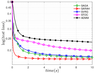
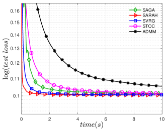
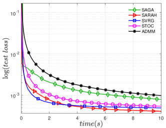
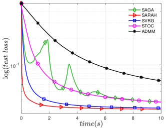
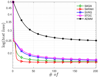
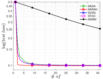
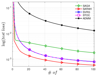
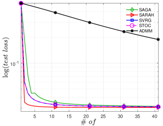
In Figure 1, we give the results of different methods for test loss with the same running time. Figure 2 shows that the results of different algorithms for solving the problem (4.1) by using the same number of epoch, where each epoch estimates $n$ component gradients. We can see that the SARAH-ADMM always has the lowest test-loss and it also faster than SAGA-ADMM, SVRG-ADMM, STOC-ADMM and ADMM. We also note that SVRG-ADMM and SAGA-ADMM have the similar behaviors and both algorithms are faster than the deterministic ADMM.

(a) a8a

(b) ijcnn

(c) mushrooms

(d) w3a

Figure 2: Test loss for different methods with the same number of epoch.

4.2 Wavelet Frame Based 2D CT Reconstruction

In the past decade, wavelet frame based models have been widely used for image denoising, reconstruction and restoration [52]. Wavelet frame based approaches utilized the observation that images can often be sparsely approximated by properly designed wavelet frames. At the same time, a wavelet frame based $L_{0}$ minimization model has presented its advantages [5]. In this subsection, we use the wavelet frame based $L_{0}$ norm as a regularization term for 2D CT reconstruction problem:

$$\min_{x}{{\frac{\raisebox{0.41669pt}{\footnotesize$1$}}{\raisebox{-1.24994pt}{\footnotesize$n$}}}}\sum_{i=1}^{n}(\mathcal{R}_{i}x-b_{i})^{2}+\sum_{i}\lambda_{i}\|(\mathcal{W}x)_{i}\|_{0},$$

where $\mathcal{R}$ is the Radon operator generated by using fan beam scanning geometry [20] and the number of detectors is 512. We generate the observed data in the following two cases:

Case 1. Let the number of viewers be 360, then the dimension of observed data $b$ is 184320. We add the white noise with mean 0 variance 0.5 on the measured data $b$.

Case 2. Let the number of viewers be 60, then the dimension of observed data $b$ is 30720. We add the white noise with mean 0 variance 0.15 on the measured data $b$.

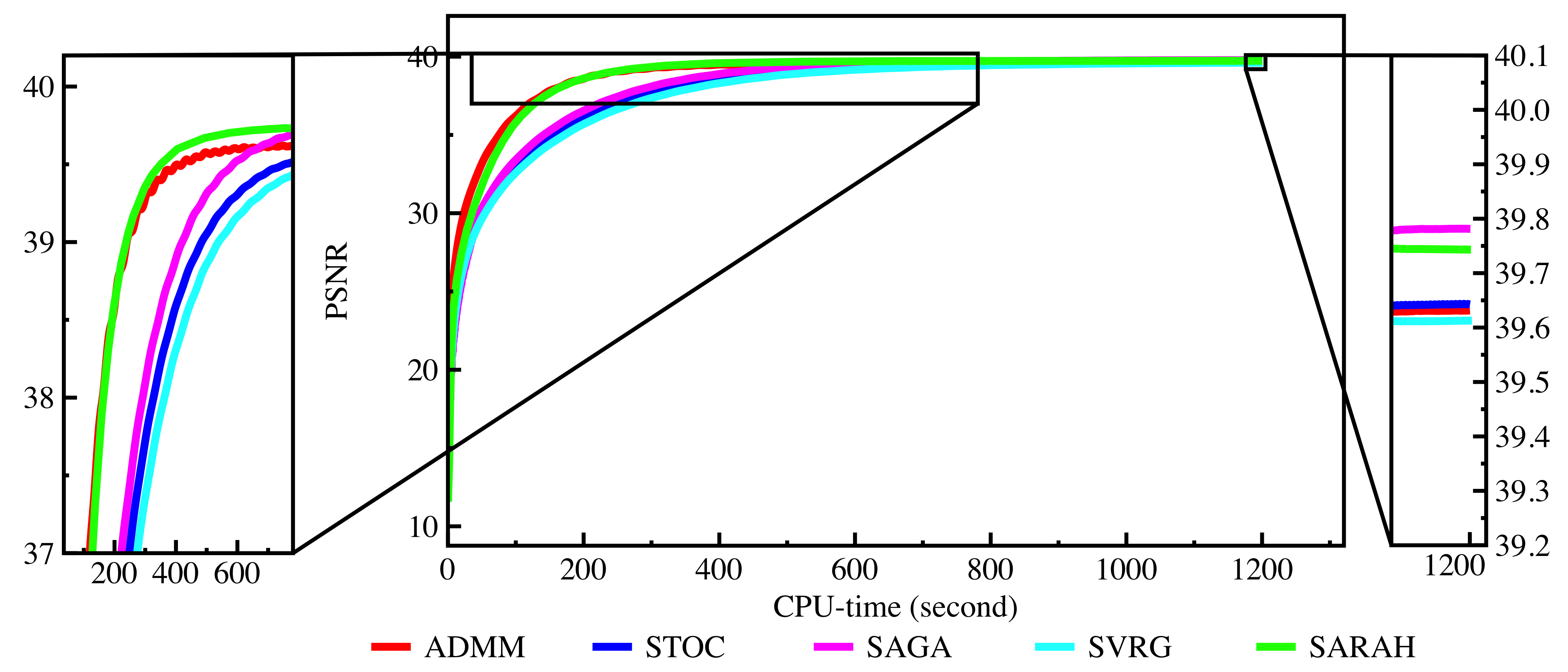
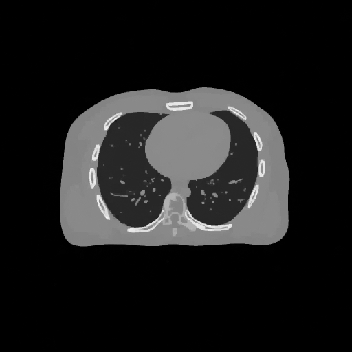
We solve the above two cases by using SARAH-ADMM, SAGA-ADMM, SVRG-ADMM, STOC-ADMM and deterministic ADMM. In two cases, we set $\lambda=1e-5$ and $\beta=1e-4$. In each algorithm, $\tau$ and batch size are taken to be the value that makes the experiment result best. Figure 3 shows how the PSNR of images changes as the running time increases. As we can see in the magnified image on the left, ADMM and SARAH-ADMM can achieve relatively high PSNR in the shortest time. From the magnified image on the right and Figure 4, we see that the final PSNR of SARAH-ADMM is relatively high. The SAGA-ADMM can also reach a relatively high PSNR, but its speed is relatively slow. In Figure 4 and Figure 5, we give the final CT image reconstruction results for Case 1 and Case 2 respectively, from which we see that SARAH-ADMM gets better results than other methods.

Figure 3: PSNR results of different methods for Case 1

(a) Ground truth

(b) STOC= 39.64

(c) SVRG= 39.61

(d) ADMM = 39.63

(e) SAGA= 39.78

(f) SARAH= 39.74

Figure 4: Final reconstruction images of different methods for Case 1.

(a) Ground truth

(b) STOC= 38.27

(c) SVRG= 37.99

(d) ADMM = 37.99

(e) SAGA= 37.54

(f) SARAH= 38.71

Figure 5: Final reconstruction images of different methods for Case 2.

4.3 TV-$L_{0}$ for 3D CT Reconstruction

In this subsection, we consider the 3D CT reconstruction problem by using TV-$L_{0}$ norm as the regularization :

$$\min_{x}{{\frac{\raisebox{0.41669pt}{\footnotesize$1$}}{\raisebox{-1.24994pt}{\footnotesize$n$}}}}\sum_{i=1}^{n}(\mathcal{R}_{i}x-b_{i})^{2}+\lambda\|\nabla x\|_{0},$$

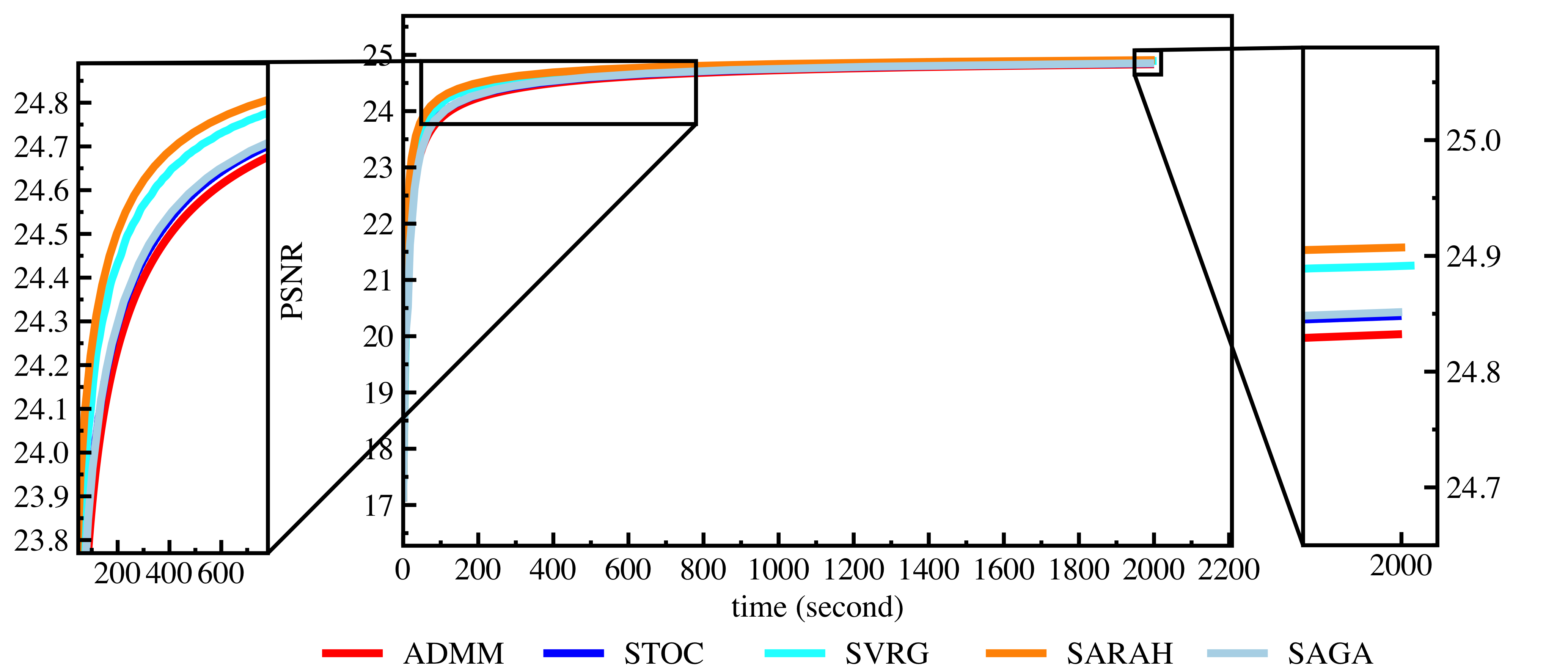
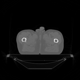
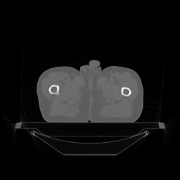
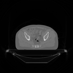
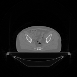
where $\mathcal{R}$ is the Radon transform generated by using the cone beam scanning geometry [20], the detectors plane is $512\times 384$ and the number of viewers is 668. The size of 3D image which will be constructed is $256\times 256\times 64$. Then the size of observed data $b$ is 131334144, that is to say, $n$ is considerably large. Here, we compare SARAH-ADMM with SVRG-ADMM, STOC-ADMM and ADMM. We let $\lambda=\mathcal{O}(1e-2)$, $\beta=\mathcal{O}(1e-11)$ and $\sigma=0.95$. The parameters $\tau$ and batch size $b$ are selected so that each algorithm can achieve the best result. Figure 6 shows how the PSNR of 3D images changes as the running time increases. Figure 7, 8 present the images and PSNR of the 15th, 55th slices of the 3D image. We can see that SARAH-ADMM and SVRG-ADMM can achieve a better PSNR in a relatively short time. However, STOC-ADMM and ADMM are relatively slow. From Figure 7 and Figure 8, we also can see that the final PSNR of SARAH-ADMM and SVRG-ADMM is better.

Figure 6: PSNR for different methods

(a) Ground truth

(b) STOC= 49.05

(c) SVRG= 52.37

(d) ADMM = 47.82

(e) SAGA= 49.39

(f) SARAH= 53.58

Figure 7: Final reconstruction image of different methods for the 15th slice.

(a) Ground truth

(b) STOC= 46.86

(c) SVRG= 49.99

(d) ADMM = 45.78

(e) SAGA= 47.12

(f) SARAH= 51.60

Figure 8: Final reconstruction image of different methods for the 55th slice.

5 Conclusion

In this paper, we propose stochastic version ADMM which incorporates a class of variance reduction gradient estimators including SAGA and SARAH. Based on an MSE bound and KL property, we establish the convergence for the proposed algorithm. We demonstrate the performance of the proposed algorithm with SARAH, SAGA gradient estimators for three different problems: graphed-guided fused lasso, wavelet frame based 2D CT reconstruction and TV-$L_{0}$ for 3D CT reconstruction.

Acknowledgement

This work was supported by NSFC (No.11771288) and National key research and development program (No.2017YFB0202902). We thank the Student Innovation Center at Shanghai Jiao Tong University for providing us the computing services. Jingwei Liang was partly supported by Leverhulme Trust and Newton Trust.

Appendix A Proofs of main theorems

A.1 Properties of SAGA gradient approximation

The MSE bound, geometric decay and convergence of the SAGA estimator have been established in [10], we present them here for the sake of convenience.

Lemma A.1 (MSE bound).

The SAGA estimator satisfies

$$\mathbb{E}_{t}\|\widetilde{\nabla}H(x_{t})-\nabla H(x_{t})\|^{2}\leq{{\frac{\raisebox{0.41669pt}{\footnotesize$1$}}{\raisebox{-1.24994pt}{\footnotesize$bn$}}}}\sum\nolimits_{i=1}^{n}\|\nabla H_{i}(x_{t})-\nabla H_{i}(\varphi_{t}^{i})\|^{2},$$ (A.1)

as well as

$$\mathbb{E}_{t}\|\widetilde{\nabla}H(x_{t})-\nabla H(x_{t})\|\leq{{\frac{\raisebox{0.41669pt}{\footnotesize$1$}}{\raisebox{-1.24994pt}{\footnotesize$\sqrt{bn}$}}}}\sum\nolimits_{i=1}^{n}\|\nabla H_{i}(x_{t})-\nabla H_{i}(\varphi_{t}^{i})\|.$$ (A.2)

• According to the definition of SAGA operator (2.2), we have

  $$\mathbb{E}_{t}\|\widetilde{\nabla}H(x_{t})-\nabla H(x_{t})\|^{2} =\mathbb{E}_{t}\|{{\frac{\raisebox{0.41669pt}{\footnotesize$1$}}{\raisebox{-1.24994pt}{\footnotesize$b$}}}}\mathbin{\scalebox{1.125}{$\sum$}}_{j\in J_{t}}(\nabla H_{j}(x_{t})-\nabla H_{j}(\varphi_{t}^{j}))+{{\frac{\raisebox{0.41669pt}{\footnotesize$1$}}{\raisebox{-1.24994pt}{\footnotesize$n$}}}}\mathbin{\scalebox{1.125}{$\sum$}}_{i=1}^{n}\nabla H_{i}(\varphi_{t}^{i})-\nabla H(x_{t})\|^{2}$$

  $$={{\frac{\raisebox{0.41669pt}{\footnotesize$1$}}{\raisebox{-1.24994pt}{\footnotesize$b^{2}$}}}}\mathbb{E}_{t}\sum\nolimits_{j\in J_{t}}\|\nabla H_{j}(x_{t})-\nabla H_{j}(\varphi_{t}^{j})\|^{2}$$

  $$={{\frac{\raisebox{0.41669pt}{\footnotesize$1$}}{\raisebox{-1.24994pt}{\footnotesize$bn$}}}}\sum\nolimits_{i=1}^{n}\|\nabla H_{i}(x_{t})-\nabla H_{i}(\varphi_{t}^{i})\|^{2},$$

  where the second equality is obtained by $\mathbb{E}( \xi-\mathbb{E}\xi)^{2}=\mathbb{E}\xi^{2}$. By the Jensen inequality, we can say that

  $$\mathbb{E}_{t}\|\widetilde{\nabla}H(x_{t})-\nabla H(x_{t})\| \leq\sqrt{\mathbb{E}_{t}\|\widetilde{\nabla}H(x_{t})-\nabla H(x_{t})\|^{2}}$$

  $$\leq{{\frac{\raisebox{0.41669pt}{\footnotesize$1$}}{\raisebox{-1.24994pt}{\footnotesize$\sqrt{bn}$}}}}\sqrt{\mathbin{\scalebox{1.125}{$\sum$}}_{i=1}^{n}\|\nabla H_{i}(x_{t})-\nabla H_{i}(\varphi_{t}^{i})\|^{2}}$$

  $$\leq{{\frac{\raisebox{0.41669pt}{\footnotesize$1$}}{\raisebox{-1.24994pt}{\footnotesize$\sqrt{bn}$}}}}\sum\nolimits_{i=1}^{n}\|\nabla H_{i}(x_{t})-\nabla H_{i}(\varphi_{t}^{i})\|.$$

  Hence, we get (A.1) and (A.2). ∎

Lemma A.2 (Geometric decay).

For the SAGA estimator, we define

$$\Upsilon_{t+1}={{\frac{\raisebox{0.41669pt}{\footnotesize$1$}}{\raisebox{-1.24994pt}{\footnotesize$bn$}}}}\sum\nolimits_{i=1}^{n}\|\nabla H_{i}(x_{t+1})-\nabla H_{i}(\varphi_{t+1}^{i})\|^{2},$$

$$\Gamma_{t+1}={{\frac{\raisebox{0.41669pt}{\footnotesize$1$}}{\raisebox{-1.24994pt}{\footnotesize$\sqrt{bn}$}}}}\sum\nolimits_{i=1}^{n}\|\nabla H_{i}(x_{t+1})-\nabla H_{i}(\varphi_{t+1}^{i})\|.$$

Then the sequence $\{\Upsilon_{t}\}_{t\geq 1}$ decays geometrically:

$$\mathbb{E}_{t}{\Upsilon_{t+1}}\leq(1-\rho)\Upsilon_{t}+V_{\Upsilon}\mathbb{E}_{t}\|x_{t+1}-x_{t}\|^{2},$$

where $\rho={{\frac{\raisebox{0.29167pt}{\footnotesize$b$}}{\raisebox{-0.87495pt}{\footnotesize$n$}}}}$ and $V_{\Upsilon}=\frac{nL^{2}}{bn-1}$.

• Now, we show that $\mathbb{E}\Upsilon_{t+1}$ is decreasing at a geometric rate by applying the inequality $\|a-c\|^{2}\leq(1+\delta)\|a-b\|^{2}+(1+\delta^{-1})\|b-c\|^{2}$ twice.

  $$\mathbb{E}_{t}\Upsilon_{t+1} ={{\frac{\raisebox{0.41669pt}{\footnotesize$1$}}{\raisebox{-1.24994pt}{\footnotesize$bn$}}}}\mathbb{E}_{t}\big{[}\mathbin{\scalebox{1.125}{$\sum$}}_{i=1}^{n}\|\nabla H_{i}(x_{t+1})-\nabla H_{i}(\varphi_{t+1}^{i})\|^{2}\big{]}$$

  $$\leq{{\frac{\raisebox{0.41669pt}{\footnotesize$1$}}{\raisebox{-1.24994pt}{\footnotesize$bn$}}}}\sum_{i=1}^{n}\mathbb{E}_{t}\|\nabla H_{i}(x_{t+1})-\nabla H_{i}(x_{t})+\nabla H_{i}(x_{t})-\nabla H_{i}(\varphi_{t+1}^{i})\|^{2}$$

  $$\leq{{\frac{\raisebox{0.41669pt}{\footnotesize$1+\delta^{-1}$}}{\raisebox{-1.24994pt}{\footnotesize$bn$}}}}\mathbb{E}_{t}\sum_{i=1}^{n}\|\nabla H_{i}(x_{t+1})-\nabla H_{i}(x_{t})\|^{2}+{{\frac{\raisebox{0.41669pt}{\footnotesize$1+\delta$}}{\raisebox{-1.24994pt}{\footnotesize$bn$}}}}\mathbb{E}_{t}\sum_{i=1}^{n}\|\nabla H_{i}(x_{t})-\nabla H_{i}(\varphi_{t+1}^{i})\|^{2}$$

  $$\leq{{\frac{\raisebox{0.41669pt}{\footnotesize$1+\delta^{-1}$}}{\raisebox{-1.24994pt}{\footnotesize$bn$}}}}\mathbb{E}_{t}\sum_{i=1}^{n}\|\nabla H_{i}(x_{t+1})-\nabla H_{i}(x_{t})\|^{2}+{{\frac{\raisebox{0.41669pt}{\footnotesize$(1+\delta)(1-{{\frac{\raisebox{0.23334pt}{\footnotesize$b$}}{\raisebox{-0.69997pt}{\footnotesize$n$}}}})$}}{\raisebox{-1.24994pt}{\footnotesize$bn$}}}}\sum_{i=1}^{n}\|\nabla H_{i}(x_{t})-\nabla H_{i}(\varphi_{t}^{i})\|^{2}$$

  $$\leq{{\frac{\raisebox{0.41669pt}{\footnotesize$(1+\delta)(1-{{\frac{\raisebox{0.23334pt}{\footnotesize$b$}}{\raisebox{-0.69997pt}{\footnotesize$n$}}}})$}}{\raisebox{-1.24994pt}{\footnotesize$bn$}}}}\sum_{i=1}^{n}\|\nabla H_{i}(x_{t})-\nabla H_{i}(\varphi_{t}^{i})\|^{2}+{{\frac{\raisebox{0.41669pt}{\footnotesize$(1+\delta^{-1})L^{2}$}}{\raisebox{-1.24994pt}{\footnotesize$b$}}}}\mathbb{E}_{t}\|x_{t+1}-x_{t}\|^{2}.$$

  Choosing $\delta=bn-1$, we have $\frac{(1+\delta)(1-\frac{b}{n})}{bn}=1-\frac{b}{n}<1$. Then we can get the geometric decay of $\{\Upsilon_{t}\}_{t\geq 1}$:

  $$\mathbb{E}_{t}{\Upsilon_{t+1}}\leq(1-\rho)\Upsilon_{t}+V_{r}\mathbb{E}_{t}\|x_{t+1}-x_{t}\|^{2},$$

  where $\rho=\frac{b}{n}$ and $V_{\Upsilon}=\frac{nL^{2}}{bn-1}$. This completes the proof. ∎

Lemma A.3 (Convergence of estimator).

If $\lim_{t\to\infty}\mathbb{E}\|x_{t}-x_{t-1}\|=0,$ it follows that $\mathbb{E}\Upsilon_{t}\to 0$ and $\mathbb{E}\Gamma_{t}\to 0$.

• From the conclusion in Lemma A.2, we can see that if $\mathbb{E}\|x_{t}-x_{t-1}\|^{2}\to 0$, then so do $\Upsilon_{t}$ and $\Gamma_{t}$. First, we show that $\sum_{i=1}^{n}\mathbb{E}\|\nabla H_{i}(x_{t})-H_{i}(\varphi_{t}^{i})\|^{2}\to 0.$
  

  $$\sum_{i=1}^{n}\mathbb{E}\|\nabla H_{i}(x_{t})-\nabla H_{i}(\varphi_{t}^{i})\|^{2} \leq L^{2}\sum_{i=1}^{n}\mathbb{E}\|x_{t}-\varphi_{t}^{i}\|^{2}$$

  $$\leq L^{2}n(1+{{\frac{\raisebox{0.41669pt}{\footnotesize$2n$}}{\raisebox{-1.24994pt}{\footnotesize$b$}}}})\mathbb{E}\|x_{t}-x_{t-1}\|^{2}+(1+{{\frac{\raisebox{0.41669pt}{\footnotesize$b$}}{\raisebox{-1.24994pt}{\footnotesize$2n$}}}})\sum_{i=1}^{n}\mathbb{E}\|x_{t-1}-\varphi_{t}^{i}\|^{2}$$

  $$\leq L^{2}n(1+{{\frac{\raisebox{0.41669pt}{\footnotesize$2n$}}{\raisebox{-1.24994pt}{\footnotesize$b$}}}})\mathbb{E}\|x_{t}-x_{t-1}\|^{2}+(1+{{\frac{\raisebox{0.41669pt}{\footnotesize$b$}}{\raisebox{-1.24994pt}{\footnotesize$2n$}}}})(1-{{\frac{\raisebox{0.41669pt}{\footnotesize$b$}}{\raisebox{-1.24994pt}{\footnotesize$n$}}}})\sum_{i=1}^{n}\mathbb{E}\|x_{t-1}-\varphi_{t-1}^{i}\|^{2}$$

  $$\leq L^{2}n(1+{{\frac{\raisebox{0.41669pt}{\footnotesize$2n$}}{\raisebox{-1.24994pt}{\footnotesize$b$}}}})\mathbb{E}\|x_{t}-x_{t-1}\|^{2}+(1-{{\frac{\raisebox{0.41669pt}{\footnotesize$b$}}{\raisebox{-1.24994pt}{\footnotesize$2n$}}}})\sum_{i=1}^{n}\mathbb{E}\|x_{t-1}-\varphi_{t-1}^{i}\|^{2}$$

  $$\leq L^{2}n(1+{{\frac{\raisebox{0.41669pt}{\footnotesize$2n$}}{\raisebox{-1.24994pt}{\footnotesize$b$}}}})\sum_{l=1}^{t}(1-{{\frac{\raisebox{0.41669pt}{\footnotesize$b$}}{\raisebox{-1.24994pt}{\footnotesize$2n$}}}})^{t-l}\mathbb{E}\|x_{l}-x_{l-1}\|^{2},$$

  where the third inequality is obtained by using the definition of $\varphi_{t}$ in Definition 2.2. Furthermore, because $\|x_{t}-x_{t-1}\|^{2}\to 0,$ it is clear that the bound on the right goes to zero as $t\to\infty.$ The fact that $\Gamma_{t}\to 0$ follows similarly:

  $$\sum_{i=1}^{n}\mathbb{E}\|\nabla H_{i}(x_{t})-\nabla H_{i}(\varphi_{t}^{i})\| \leq L\sum\nolimits_{i=1}^{n}\mathbb{E}\|x_{t}-\varphi_{t}^{i}\|$$

  $$\leq nL\|x_{t}-x_{t-1}\|+\sum\nolimits_{i=1}^{n}\mathbb{E}\|x_{t-1}-\varphi_{t}^{i}\|$$

  $$\leq nL\|x_{t}-x_{t-1}\|+(1-{{\frac{\raisebox{0.41669pt}{\footnotesize$b$}}{\raisebox{-1.24994pt}{\footnotesize$n$}}}})\sum\nolimits_{i=1}^{n}\mathbb{E}\|x_{t-1}-\varphi_{t-1}^{i}\|$$

  $$\leq nL\sum\nolimits_{l=1}^{t}(1-{{\frac{\raisebox{0.41669pt}{\footnotesize$b$}}{\raisebox{-1.24994pt}{\footnotesize$n$}}}})^{t-l}\mathbb{E}\|x_{t}-x_{t-1}\|.$$

  As $\|x_{t}-x_{t-1}\|\to 0,$ it follows that the bound on the right goes to zero as $t\to\infty$, so $\Gamma_{t}\to 0$. ∎

A.2 Properties of SARAH gradient approximation

Lemma A.4 (MSE bound).

The SARAH gradient estimator satisfies

$$\mathbb{E}_{t}\|\widetilde{\nabla}H(x_{t})-\nabla H(x_{t})\|^{2}\leq\big{(}{1-{{\frac{\raisebox{0.41669pt}{\footnotesize$1$}}{\raisebox{-1.24994pt}{\footnotesize$p$}}}}}\big{)}\|\widetilde{\nabla}H(x_{t-1})-\nabla H(x_{t-1})\|^{2}+{{\frac{\raisebox{0.41669pt}{\footnotesize$L^{2}$}}{\raisebox{-1.24994pt}{\footnotesize$b$}}}}\|x_{t}-x_{t-1}\|^{2},$$

as well as

$$\mathbb{E}_{t}\|\widetilde{\nabla}H(x_{t})-\nabla H(x_{t})\|\leq\sqrt{1-\tfrac{1}{p}}\|\widetilde{\nabla}H(x_{t-1})-\nabla H(x_{t-1})\|+{{\frac{\raisebox{0.41669pt}{\footnotesize$L$}}{\raisebox{-1.24994pt}{\footnotesize$\sqrt{b}$}}}}\|x_{t}-x_{t-1}\|.$$

• By using the definition of SARAH estimator in Definition 2.3, we have

  $$\mathbb{E}_{t,p}\widetilde{\nabla}H(x_{t}) =\mathbb{E}_{t,p}\big{[}{{\frac{\raisebox{0.41669pt}{\footnotesize$1$}}{\raisebox{-1.24994pt}{\footnotesize$b$}}}}\mathbin{\scalebox{1.125}{$\sum$}}_{j\in J_{t}}\nabla H_{j}(x_{t})-\nabla H_{j}(x_{t-1})+\widetilde{\nabla}H(x_{t-1})\big{]}$$

  $$=\nabla H(x_{t})-\nabla H(x_{t-1})+\widetilde{\nabla}H(x_{t-1}).$$

  In the following, we begin with a bound on $\mathbb{E}_{t,p}\|\widetilde{\nabla}H(x_{t})-\nabla H(x_{t})\|^{2}$.

  $$\mathbb{E}_{t,p}\|\widetilde{\nabla}H(x_{t})-\nabla H(x_{t})\|^{2}$$

  $$=\mathbb{E}_{t,p}\|\widetilde{\nabla}H(x_{t-1})-\nabla H(x_{t-1})+\nabla H(x_{t-1})-\nabla H(x_{t})+\widetilde{\nabla}H(x_{t})-\widetilde{\nabla}H(x_{t-1})\|^{2}$$

  $$=\|\widetilde{\nabla}H(x_{t-1})-\nabla H(x_{t-1})\|^{2}+\|\nabla H(x_{t-1})-\nabla H(x_{t})\|^{2}+\mathbb{E}_{t,p}\|\widetilde{\nabla}H(x_{t})-\widetilde{\nabla}H(x_{t-1})\|^{2}$$

  $$\qquad+2\langle\nabla H(x_{t-1})-\widetilde{\nabla}H(x_{t-1}),\nabla H(x_{t})-\nabla H(x_{t-1})\rangle$$

  $$\qquad-2\langle\nabla H(x_{t-1})-\widetilde{\nabla}H(x_{t-1}),\mathbb{E}_{t,p}[\widetilde{\nabla}H(x_{t})-\widetilde{\nabla}H(x_{t-1})]\rangle$$

  $$\qquad-2\langle\nabla H(x_{t})-\nabla H(x_{t-1}),\mathbb{E}_{t,p}[\widetilde{\nabla}H(x_{t})-\widetilde{\nabla}H(x_{t-1})]\rangle.$$

  To simplify the inner product terms, we use the fact that

  $$\mathbb{E}_{t,p}[\widetilde{\nabla}H(x_{t})-\widetilde{\nabla}H(x_{t-1})]=\nabla H(x_{t})-\nabla H(x_{t-1}).$$

  With this equality established, we see that the second inner product is equal to

  $$2\langle\nabla H(x_{t-1})-\widetilde{\nabla}H(x_{t-1}),\mathbb{E}_{t,p}[\widetilde{\nabla}H(x_{t})-\widetilde{\nabla}H(x_{t-1})]\rangle=2\langle\nabla H(x_{t-1})-\widetilde{\nabla}H(x_{t-1}),\nabla H(x_{t})-\nabla H(x_{t-1})\rangle.$$

  The third inner product is equal to

  $$2\langle\nabla H(x_{t})-\nabla H(x_{t-1}),\mathbb{E}_{t,p}[\widetilde{\nabla}H(x_{t})-\widetilde{\nabla}H(x_{t-1})]\rangle=2\|\nabla H(x_{t})-\nabla H(x_{t-1})\|^{2}.$$

  Consequently, we have

  $$\mathbb{E}_{t,p}\|\widetilde{\nabla}H(x_{t})-\nabla H(x_{t})\|^{2}$$

  $$\leq\|\widetilde{\nabla}H(x_{t-1})-\nabla H(x_{t-1})\|^{2}-\|\nabla H(x_{t})-\nabla H(x_{t-1})\|^{2}+\mathbb{E}_{t,p}\|\widetilde{\nabla}H(x_{t})-\widetilde{\nabla}H(x_{t-1})\|^{2}$$

  $$\leq\|\widetilde{\nabla}H(x_{t-1})-\nabla H(x_{t-1})\|^{2}+\mathbb{E}_{t,p}\|\widetilde{\nabla}H(x_{t})-\widetilde{\nabla}H(x_{t-1})\|^{2}.$$

  We can bound the second term by computing the expectation,

  $$\mathbb{E}_{t,p}\|\widetilde{\nabla}H(x_{t})-\widetilde{\nabla}H(x_{t-1})\|^{2} =\mathbb{E}_{t,p}\|{{\frac{\raisebox{0.41669pt}{\footnotesize$1$}}{\raisebox{-1.24994pt}{\footnotesize$b$}}}}\big{(}{\mathbin{\scalebox{1.125}{$\sum$}}_{j\in J_{t}}\nabla H_{j}(x_{t})-\nabla H_{j}(x_{t-1})}\big{)}\|^{2}$$

  $$\leq{{\frac{\raisebox{0.41669pt}{\footnotesize$1$}}{\raisebox{-1.24994pt}{\footnotesize$b^{2}$}}}}\mathbb{E}_{t,p}\big{[}\mathbin{\scalebox{1.125}{$\sum$}}_{j\in J_{t}}\|\nabla H_{j}(x_{t})-\nabla H_{j}(x_{t-1})\|^{2}\big{]}$$

  $$={{\frac{\raisebox{0.41669pt}{\footnotesize$1$}}{\raisebox{-1.24994pt}{\footnotesize$bn$}}}}\sum_{i=1}^{n}\|\nabla H_{i}(x_{t})-\nabla H_{i}(x_{t-1})\|^{2}.$$

  Then we have

  $$\mathbb{E}_{t,p}\|\widetilde{\nabla}H(x_{t})-\nabla H(x_{t})\|^{2}\leq\|\widetilde{\nabla}H(x_{t-1})-\nabla H(x_{t-1})\|^{2}+{{\frac{\raisebox{0.41669pt}{\footnotesize$1$}}{\raisebox{-1.24994pt}{\footnotesize$bn$}}}}\sum_{i=1}^{n}\|\nabla H_{i}(x_{t})-\nabla H_{i}(x_{t-1})\|^{2}.$$

  When the full gradient is computed, the MSE is equal to zero, so

  $$\mathbb{E}_{t}\|\widetilde{\nabla}H(x_{t})-\nabla H(x_{t})\|^{2} \leq\big{(}{1-{{\frac{\raisebox{0.41669pt}{\footnotesize$1$}}{\raisebox{-1.24994pt}{\footnotesize$p$}}}}}\big{)}\big{(}{\|\widetilde{\nabla}H(x_{t-1})-\nabla H(x_{t-1})\|^{2}+{{\frac{\raisebox{0.41669pt}{\footnotesize$1$}}{\raisebox{-1.24994pt}{\footnotesize$bn$}}}}\mathbin{\scalebox{1.125}{$\sum$}}_{i=1}^{n}\|\nabla H_{i}(x_{t})-\nabla H_{i}(x_{t-1})\|^{2}}\big{)}$$

  $$\leq\big{(}{1-{{\frac{\raisebox{0.41669pt}{\footnotesize$1$}}{\raisebox{-1.24994pt}{\footnotesize$p$}}}}}\big{)}\|\widetilde{\nabla}H(x_{t-1})-\nabla H(x_{t-1})\|^{2}+{{\frac{\raisebox{0.41669pt}{\footnotesize$L^{2}$}}{\raisebox{-1.24994pt}{\footnotesize$b$}}}}\|x_{t}-x_{t-1}\|^{2}.$$

  Due to Jensen’s inequality:

  $$\mathbb{E}_{t}\|\widetilde{\nabla}H(x_{t})-\nabla H(x_{t})\| \leq\sqrt{\mathbb{E}_{t}\|\widetilde{\nabla}H(x_{t})-\nabla H(x_{t})\|^{2}}$$

  $$\leq\sqrt{(1-\tfrac{1}{p})\|\widetilde{\nabla}H(x_{t-1})-\nabla H(x_{t-1})\|^{2}+{{\frac{\raisebox{0.41669pt}{\footnotesize$L^{2}$}}{\raisebox{-1.24994pt}{\footnotesize$b$}}}}\|x_{t}-x_{t-1}\|^{2}}$$

  $$\leq\sqrt{1-\tfrac{1}{p}}\|\widetilde{\nabla}H(x_{t-1})-\nabla H(x_{t-1})\|+{{\frac{\raisebox{0.41669pt}{\footnotesize$L$}}{\raisebox{-1.24994pt}{\footnotesize$\sqrt{b}$}}}}\|x_{t}-x_{t-1}\|.$$

  This completes the proof. ∎

Lemma A.5 (Geometric decay).

For the SARAH gradient estimator, we define

$$\Upsilon_{t+1}=\|\widetilde{\nabla}H(x_{t})-\nabla H(x_{t})\|^{2},$$ (A.4a)

$$\Gamma_{t+1}=\|\widetilde{\nabla}H(x_{t})-\nabla H(x_{t})\|.$$ (A.4b)

Then the sequence $\{\Upsilon_{t}\}_{t\geq 1}$ decays geometrically:

$$\mathbb{E}_{t}{\Upsilon_{t+1}}\leq(1-\rho)\Upsilon_{t}+V_{\Upsilon}\mathbb{E}_{t}\|x_{t}-x_{t-1}\|^{2},$$ (A.5)

where $\rho={{\frac{\raisebox{0.29167pt}{\footnotesize$1$}}{\raisebox{-0.87495pt}{\footnotesize$p$}}}}$ and $V_{r}={{\frac{\raisebox{0.29167pt}{\footnotesize$L^{2}$}}{\raisebox{-0.87495pt}{\footnotesize$b$}}}}$.

• This is a direct result of Lemma A.4. ∎

Lemma A.6 (Convergence of estimator).

If $\lim_{t\to\infty}\mathbb{E}\|x_{t}-x_{t-1}\|=0,$ it follows that $\mathbb{E}\Upsilon_{t}\to 0$ and $\mathbb{E}\Gamma_{t}\to 0$.

• By (A.5) we have

  $$\mathbb{E}\Upsilon_{t}\leq(1-{{\frac{\raisebox{0.41669pt}{\footnotesize$1$}}{\raisebox{-1.24994pt}{\footnotesize$p$}}}})\mathbb{E}\Upsilon_{t-1}+{{\frac{\raisebox{0.41669pt}{\footnotesize$L^{2}$}}{\raisebox{-1.24994pt}{\footnotesize$b$}}}}\mathbb{E}\|x_{t}-x_{t-1}\|^{2}\leq{{\frac{\raisebox{0.41669pt}{\footnotesize$L^{2}$}}{\raisebox{-1.24994pt}{\footnotesize$b$}}}}\sum_{l=1}^{t}(1-{{\frac{\raisebox{0.41669pt}{\footnotesize$1$}}{\raisebox{-1.24994pt}{\footnotesize$p$}}}})^{t-l}\mathbb{E}\|x_{l}-x_{l-1}\|^{2}.$$

  It implies $\mathbb{E}\Upsilon_{t}\to 0.$ By Jensen’s inequality, we have $\mathbb{E}\Gamma_{t}\to 0$ as well. ∎

A.3 Proofs of main theorems

Before giving the proof of Theorem 3.2, we first show that the sequence $\{\Psi_{t}\}$ is bounded from below in the following lemma, which will be used in the proof of Theorem 3.2. Recall

$$\Phi(x,z,u,x^{\prime},u^{\prime})\stackrel{{\scriptstyle{\mathrm{def}}}}{{=}}L_{\beta}(x,z,u)+{{\frac{\raisebox{0.41669pt}{\footnotesize$4(1-\sigma)$}}{\raisebox{-1.24994pt}{\footnotesize$\sigma^{2}\beta\lambda_{m}$}}}}\|A^{T}(u-u^{\prime})+\sigma B(x-x^{\prime})\|^{2}+{{\frac{\raisebox{0.41669pt}{\footnotesize$8(\sigma\tau+L)^{2}$}}{\raisebox{-1.24994pt}{\footnotesize$\sigma\beta\lambda_{m}$}}}}\|x-x^{\prime}\|^{2}$$ (A.6)

$$\Phi_{t}\stackrel{{\scriptstyle{\mathrm{def}}}}{{=}}\Phi(x_{t},z_{t},u_{t},x_{t-1},u_{t-1}),\,\,\,\,X_{t}=(x_{t},z_{t},u_{t},x_{t-1},u_{t-1}),\,\,\,\,X^{*}=(x^{*},z^{*},u^{*},x^{*},u^{*}).$$

We also denote $\underline{\Phi}\stackrel{{\scriptstyle{\mathrm{def}}}}{{=}}\inf_{(x,z)}\{F(z)+H(x)\}>-\infty.$

Lemma A.7.

Suppose that (a1) of Assumption 3.1 is satisfied and $\{x_{t},z_{t},u_{t}\}_{t\geq 0}$ is a sequence generated by Algorithm 1. Then the sequence $\{\Psi_{t}\}_{t\geq 0}$ is bounded from below.

• We show that $\underline{\Phi}$ is a lower bound of $\{\Psi_{t}\}_{t\geq 1}$. Suppose by contradiction that there exists $t_{0}\geq 1$ such that $\Psi_{t_{0}}-\underline{\Phi}<0.$ According to (3.2), for any $T\geq t_{0}$,

  $$\sum_{t=1}^{T}\mathbb{E}(\Psi_{t}-\underline{\Phi})\leq\sum_{t=1}^{t_{0}-1}\mathbb{E}(\Psi_{t}-\Phi)+(T-t_{0}+1)(\Psi_{t_{0}}-\underline{\Phi}),$$

  which implies that

  $$\lim_{T\to\infty}\sum_{t=1}^{T}\mathbb{E}(\Psi_{t}-\underline{\Phi})=-\infty.$$

  On the other hand, for any $t\geq 1$ it holds that

  $$\Psi_{t}-\underline{\Phi} \geq F(z_{t})+H(x_{t})+\langle u_{t},Ax_{t}-z_{t}\rangle-\underline{\Phi}$$

  $$\geq\langle u_{t},Ax_{t}-z_{t}\rangle$$

  $$={{\frac{\raisebox{0.41669pt}{\footnotesize$1$}}{\raisebox{-1.24994pt}{\footnotesize$\sigma\beta$}}}}\langle u_{t},u_{t}-u_{t-1}\rangle$$

  $$={{\frac{\raisebox{0.41669pt}{\footnotesize$1$}}{\raisebox{-1.24994pt}{\footnotesize$2\sigma\beta$}}}}\|u_{t}\|^{2}+{{\frac{\raisebox{0.41669pt}{\footnotesize$1$}}{\raisebox{-1.24994pt}{\footnotesize$2\sigma\beta$}}}}\|u_{t}-u_{t-1}\|^{2}-{{\frac{\raisebox{0.41669pt}{\footnotesize$1$}}{\raisebox{-1.24994pt}{\footnotesize$2\sigma\beta$}}}}\|u_{t-1}\|^{2}.$$

  Therefore, for any $T\geq 1$, we have

  $$\sum_{t=1}^{T}\mathbb{E}(\Psi_{t}-\underline{\Phi})\geq{{\frac{\raisebox{0.41669pt}{\footnotesize$1$}}{\raisebox{-1.24994pt}{\footnotesize$2\sigma\beta$}}}}\sum_{t=1}^{T}\mathbb{E}\|u_{t}-u_{t-1}\|^{2}+{{\frac{\raisebox{0.41669pt}{\footnotesize$1$}}{\raisebox{-1.24994pt}{\footnotesize$2\sigma\beta$}}}}\|u_{T}\|^{2}-{{\frac{\raisebox{0.41669pt}{\footnotesize$1$}}{\raisebox{-1.24994pt}{\footnotesize$2\sigma\beta$}}}}\|u_{0}\|^{2}\geq-{{\frac{\raisebox{0.41669pt}{\footnotesize$1$}}{\raisebox{-1.24994pt}{\footnotesize$2\sigma\beta$}}}}\|u_{0}\|^{2},$$

  which leads to a contradiction. ∎

• From (1.5a) we obtain

  $$F(z_{t+1})+\langle u_{t},Ax_{t}-z_{t+1}\rangle+{{\frac{\raisebox{0.41669pt}{\footnotesize$\beta$}}{\raisebox{-1.24994pt}{\footnotesize$2$}}}}\|Ax_{t}-z_{t+1}\|^{2}\leq F(z_{t})+\langle u_{t},Ax_{t}-z_{t}\rangle+{{\frac{\raisebox{0.41669pt}{\footnotesize$\beta$}}{\raisebox{-1.24994pt}{\footnotesize$2$}}}}\|Ax_{t}-z_{t}\|^{2}.$$ (A.7)

  On the other hand, as the gradient of $H$ is Lipschitz continuous, we have

  $$H(x_{t+1})\leq H(x_{t})+\langle\nabla H(x_{t}),x_{t+1}-x_{t}\rangle+{{\frac{\raisebox{0.41669pt}{\footnotesize$L$}}{\raisebox{-1.24994pt}{\footnotesize$2$}}}}\|x_{t+1}-x_{t}\|^{2}.$$

  By taking into consideration (1.5b), we get

  $$H(x_{t+1}) \leq H(x_{t})+\langle\widetilde{\nabla}H(x_{t}),x_{t+1}-x_{t}\rangle+{{\frac{\raisebox{0.41669pt}{\footnotesize$L$}}{\raisebox{-1.24994pt}{\footnotesize$2$}}}}\|x_{t+1}-x_{t}\|^{2}+\langle\nabla H(x_{t})-\widetilde{\nabla}H(x_{t}),x_{t+1}-x_{t}\rangle$$ (A.8)

  $$\leq H(x_{t})+\langle\tau(x_{t}-x_{t+1})-A^{T}u_{t}+\beta A^{T}(Ax_{t}-z_{t+1}),x_{t+1}-x_{t}\rangle$$

  $$\qquad+{{\frac{\raisebox{0.41669pt}{\footnotesize$L$}}{\raisebox{-1.24994pt}{\footnotesize$2$}}}}\|x_{t+1}-x_{t}\|^{2}+\langle\nabla H(x_{t})-\widetilde{\nabla}H(x_{t}),x_{t+1}-x_{t}\rangle$$

  $$\leq H(x_{t})-\tau\|x_{t+1}-x_{t}\|^{2}-\langle u_{t},A(x_{t+1}-x_{t})\rangle-\beta\langle Ax_{t}-z_{t+1},Ax_{t+1}-Ax_{t}\rangle$$

  $$\qquad+{{\frac{\raisebox{0.41669pt}{\footnotesize$L$}}{\raisebox{-1.24994pt}{\footnotesize$2$}}}}\|x_{t+1}-x_{t}\|^{2}+\langle\nabla H(x_{t})-\widetilde{\nabla}H(x_{t}),x_{t+1}-x_{t}\rangle$$

  $$\leq H(x_{t})-\langle u_{t},Ax_{t+1}-Ax_{t}\rangle+{{\frac{\raisebox{0.41669pt}{\footnotesize$\beta$}}{\raisebox{-1.24994pt}{\footnotesize$2$}}}}\|Ax_{t}-z_{t+1}\|^{2}-{{\frac{\raisebox{0.41669pt}{\footnotesize$\beta$}}{\raisebox{-1.24994pt}{\footnotesize$2$}}}}\|Ax_{t+1}-z_{t+1}\|^{2}$$

  $$\qquad-(\tau-{{\frac{\raisebox{0.41669pt}{\footnotesize$L+\beta\|A\|^{2}$}}{\raisebox{-1.24994pt}{\footnotesize$2$}}}})\|x_{t+1}-x_{t}\|^{2}+\langle\nabla H(x_{t})-\widetilde{\nabla}H(x_{t}),x_{t+1}-x_{t}\rangle,$$

  where the last inequality is due to $\langle a,b\rangle={{\frac{\raisebox{0.29167pt}{\footnotesize$1$}}{\raisebox{-0.87495pt}{\footnotesize$2$}}}}(\|a+b\|^{2}-\|a\|^{2}-\|b\|^{2})$. Rewrite (A.8), we get

  $$H(x_{t}) \geq H(x_{t+1})+\langle u_{t},Ax_{t+1}-Ax_{t}\rangle-{{\frac{\raisebox{0.41669pt}{\footnotesize$\beta$}}{\raisebox{-1.24994pt}{\footnotesize$2$}}}}\|Ax_{t}-z_{t+1}\|^{2}+{{\frac{\raisebox{0.41669pt}{\footnotesize$\beta$}}{\raisebox{-1.24994pt}{\footnotesize$2$}}}}\|Ax_{t+1}-z_{t+1}\|^{2}$$ (A.9)

  $$\qquad+(\tau-{{\frac{\raisebox{0.41669pt}{\footnotesize$L+\beta\|A\|^{2}$}}{\raisebox{-1.24994pt}{\footnotesize$2$}}}})\|x_{t+1}-x_{t}\|^{2}-\langle\nabla H(x_{t})-\widetilde{\nabla}H(x_{t}),x_{t+1}-x_{t}\rangle.$$

  Combining (A.7) and (A.9), we get

  $$F(z_{t+1})+H(x_{t+1})+\langle u_{t},Ax_{t+1}-z_{t+1}\rangle+{{\frac{\raisebox{0.41669pt}{\footnotesize$\beta$}}{\raisebox{-1.24994pt}{\footnotesize$2$}}}}\|Ax_{t+1}-z_{t+1}\|^{2}$$

  $$\qquad+(\tau-{{\frac{\raisebox{0.41669pt}{\footnotesize$L+\beta\|A\|^{2}$}}{\raisebox{-1.24994pt}{\footnotesize$2$}}}})\|x_{t+1}-x_{t}\|^{2}-\langle\nabla H(x_{t})-\widetilde{\nabla}H(x_{t}),x_{t+1}-x_{t}\rangle$$

  $$\leq F(z_{t})+H(x_{t})+\langle u_{t},Ax_{t}-z_{t}\rangle+{{\frac{\raisebox{0.41669pt}{\footnotesize$\beta$}}{\raisebox{-1.24994pt}{\footnotesize$2$}}}}\|Ax_{t}-z_{t}\|^{2}.$$

  From the equation (1.5c), we have

  $$F(z_{t+1})+H(x_{t+1})+\langle u_{t+1},Ax_{t+1}-z_{t+1}\rangle-\sigma\beta\|Ax_{t+1}-z_{t+1}\|^{2}+{{\frac{\raisebox{0.41669pt}{\footnotesize$\beta$}}{\raisebox{-1.24994pt}{\footnotesize$2$}}}}\|Ax_{t+1}-z_{t+1}\|^{2}$$

  $$\qquad+(\tau-{{\frac{\raisebox{0.41669pt}{\footnotesize$L+\beta\|A\|^{2}$}}{\raisebox{-1.24994pt}{\footnotesize$2$}}}})\|x_{t+1}-x_{t}\|^{2}-\langle\nabla H(x_{t})-\widetilde{\nabla}H(x_{t}),x_{t+1}-x_{t}\rangle$$

  $$\leq F(z_{t})+H(x_{t})+\langle u_{t},Ax_{t}-z_{t}\rangle+{{\frac{\raisebox{0.41669pt}{\footnotesize$\beta$}}{\raisebox{-1.24994pt}{\footnotesize$2$}}}}\|Ax_{t}-z_{t}\|^{2}.$$

  By adding ${{\frac{\raisebox{0.29167pt}{\footnotesize$2$}}{\raisebox{-0.87495pt}{\footnotesize$\sigma\beta$}}}}\|u_{t+1}-u_{t}\|^{2}$, we have

  $$F(z_{t+1})+H(x_{t+1})+\langle u_{t+1},Ax_{t+1}-z_{t+1}\rangle+{{\frac{\raisebox{0.41669pt}{\footnotesize$\beta$}}{\raisebox{-1.24994pt}{\footnotesize$2$}}}}\|Ax_{t+1}-z_{t+1}\|^{2}$$ (A.10)

  $$\qquad+(\tau-{{\frac{\raisebox{0.41669pt}{\footnotesize$L+\beta\|A\|^{2}$}}{\raisebox{-1.24994pt}{\footnotesize$2$}}}})\|x_{t+1}-x_{t}\|^{2}+{{\frac{\raisebox{0.41669pt}{\footnotesize$1$}}{\raisebox{-1.24994pt}{\footnotesize$\sigma\beta$}}}}\|u_{t+1}-u_{t}\|^{2}-\langle\nabla H(x_{t})-\widetilde{\nabla}H(x_{t}),x_{t+1}-x_{t}\rangle$$

  $$\leq F(z_{t})+H(x_{t})+\langle u_{t},Ax_{t}-z_{t}\rangle+{{\frac{\raisebox{0.41669pt}{\footnotesize$\beta$}}{\raisebox{-1.24994pt}{\footnotesize$2$}}}}\|Ax_{t}-z_{t}\|^{2}+{{\frac{\raisebox{0.41669pt}{\footnotesize$2$}}{\raisebox{-1.24994pt}{\footnotesize$\sigma\beta$}}}}\|u_{t+1}-u_{t}\|^{2}.$$

  Next, we will focus on estimating $\|u_{t+1}-u_{t}\|^{2}$. We can rewrite (1.5b) as

  $$\tau(x_{t}-x_{t+1}) =\widetilde{\nabla}H(x_{t})+A^{T}u_{t}+\beta A^{T}(Ax_{t+1}-z_{t+1})+\beta A^{T}A(x_{t}-x_{t+1})$$

  $$=\widetilde{\nabla}H(x_{t})+A^{T}u_{t}+{{\frac{\raisebox{0.41669pt}{\footnotesize$1$}}{\raisebox{-1.24994pt}{\footnotesize$\sigma$}}}}A^{T}(u_{t+1}-u_{t})+\beta A^{T}A(x_{t}-x_{t+1})$$

  where the last equation is due to (1.5c). After multiplying both sides by $\sigma$ and rearranging the terms, we get

  $$A^{T}u_{t+1}+\sigma B(x_{t+1}-x_{t})=(1-\sigma)A^{T}u_{t}-\sigma\widetilde{\nabla}H(x_{t}),$$

  which is equivalent to

  $$A^{T}u_{t+1}+\sigma B(x_{t+1}-x_{t})=(1-\sigma)A^{T}u_{t}-\sigma\nabla H(x_{t})-\sigma\widetilde{\nabla}H(x_{t})+\sigma\nabla H(x_{t}).$$

  Since $t$ is arbitrary, we also have

  $$A^{T}u_{t}+\sigma B(x_{t}-x_{t-1})=(1-\sigma)A^{T}u_{t-1}-\sigma\nabla H(x_{t-1})-\sigma\widetilde{\nabla}H(x_{t-1})+\sigma\nabla H(x_{t-1}).$$

  Subtracting these two identities yields

  $$A^{T}(u_{t+1}-u_{t})+\sigma B(x_{t+1}-x_{t})= (1-\sigma)A^{T}(u_{t}-u_{t-1})+\sigma B(x_{t}-x_{t-1})+\sigma\big{(}{\nabla H(x_{t-1})-\nabla H(x_{t})}\big{)}$$

  $$-\sigma\big{(}{\widetilde{\nabla}H(x_{t})-\nabla H(x_{t})}\big{)}+\sigma\big{(}{\widetilde{\nabla}H(x_{t-1})-\nabla H(x_{t-1})}\big{)}.$$

  Notice that $0<\sigma<1$ and $\|B\|\leq\tau$, by Cauchy inequality we have

  $$\|A^{T}(u_{t+1}-u_{t})+\sigma B(x_{t+1}-x_{t})\|^{2}\leq(1-\sigma)\|A^{T}(u_{t}-u_{t-1})+\sigma B(x_{t}-x_{t-1})\|^{2}$$ (A.11)

  $$\qquad+\sigma\big{(}{\|\sigma B(x_{t}-x_{t-1})\|+\|\big{(}{\nabla H(x_{t-1})-\nabla H(x_{t})}\big{)}-\big{(}{\widetilde{\nabla}H(x_{t})-\nabla H(x_{t})}\big{)}+\big{(}{\widetilde{\nabla}H(x_{t-1})-\nabla H(x_{t-1})}\big{)}\|}\big{)}^{2}$$

  $$\leq(1-\sigma)\|A^{T}(u_{t}-u_{t-1})+\sigma B(x_{t}-x_{t-1})\|^{2}+2\sigma(\sigma\tau+L)^{2}\|x_{t}-x_{t-1}\|^{2}$$

  $$\qquad+2\sigma\|\big{(}{\widetilde{\nabla}H(x_{t})-\nabla H(x_{t})}\big{)}-\big{(}{\widetilde{\nabla}H(x_{t-1})-\nabla H(x_{t-1})}\big{)}\|^{2}.$$

  On the other hand, since the linear operator $A$ is surjective, we have

  $${{\frac{\raisebox{0.41669pt}{\footnotesize$\lambda_{m}$}}{\raisebox{-1.24994pt}{\footnotesize$2$}}}}\|u_{t+1}-u_{t}\|^{2}\leq{{\frac{\raisebox{0.41669pt}{\footnotesize$1$}}{\raisebox{-1.24994pt}{\footnotesize$2$}}}}\|A^{T}(u_{t+1}-u_{t})\|^{2}\leq\|A^{T}(u_{t+1}-u_{t})+\sigma B(x_{t+1}-x_{t})\|^{2}+\sigma^{2}\tau^{2}\|x_{t+1}-x_{t}\|^{2}.\\$$

  After combining this with (A.11), we get

  $${{\frac{\raisebox{0.41669pt}{\footnotesize$\sigma\lambda_{m}$}}{\raisebox{-1.24994pt}{\footnotesize$2$}}}}\|u_{t+1}-u_{t}\|^{2}+(1-\sigma)\|A^{T}(u_{t+1}-u_{t})+\sigma B(x_{t+1}-x_{t})\|^{2}-\sigma^{3}\tau^{2}\|x_{t+1}-x_{t}\|^{2}$$

  $$\leq(1-\sigma)\|A^{T}(u_{t}-u_{t-1})+\sigma B(x_{t}-x_{t-1})\|^{2}+2\sigma(\sigma\tau+L)^{2}\|x_{t}-x_{t-1}\|^{2}$$

  $$\qquad+2\sigma\|\big{(}{\widetilde{\nabla}H(x_{t})-\nabla H(x_{t})}\big{)}-\big{(}{\widetilde{\nabla}H(x_{t-1})-\nabla H(x_{t-1})}\big{)}\|^{2}.$$

  Multiplying the above relation by ${{\frac{\raisebox{0.29167pt}{\footnotesize$4$}}{\raisebox{-0.87495pt}{\footnotesize$\sigma^{2}\beta\lambda_{m}$}}}}>0$, we have

  $${{\frac{\raisebox{0.41669pt}{\footnotesize$2$}}{\raisebox{-1.24994pt}{\footnotesize$\sigma\beta$}}}}\|u_{t+1}-u_{t}\|^{2}-{{\frac{\raisebox{0.41669pt}{\footnotesize$4\sigma\tau^{2}$}}{\raisebox{-1.24994pt}{\footnotesize$\beta\lambda_{m}$}}}}\|x_{t+1}-x_{t}\|^{2}+{{\frac{\raisebox{0.41669pt}{\footnotesize$4(1-\sigma)$}}{\raisebox{-1.24994pt}{\footnotesize$\sigma^{2}\beta\lambda_{m}$}}}}\|A^{T}(u_{t+1}-u_{t})+\sigma B(x_{t+1}-x_{t})\|^{2}$$

  $$\leq{{\frac{\raisebox{0.41669pt}{\footnotesize$4(1-\sigma)$}}{\raisebox{-1.24994pt}{\footnotesize$\sigma^{2}\beta\lambda_{m}$}}}}\|A^{T}(u_{t}-u_{t-1})+\sigma B(x_{t}-x_{t-1})\|^{2}+{{\frac{\raisebox{0.41669pt}{\footnotesize$8(\sigma\tau+L)^{2}$}}{\raisebox{-1.24994pt}{\footnotesize$\sigma\beta\lambda_{m}$}}}}\|x_{t}-x_{t-1}\|^{2}$$

  $$\qquad+{{\frac{\raisebox{0.41669pt}{\footnotesize$8$}}{\raisebox{-1.24994pt}{\footnotesize$\sigma\beta\lambda_{m}$}}}}\|\big{(}{\widetilde{\nabla}H(x_{t})-\nabla H(x_{t})}\big{)}-\big{(}{\widetilde{\nabla}H(x_{t-1})-\nabla H(x_{t-1})}\big{)}\|^{2}.$$

  Adding the resulting inequality to (A.10) yields

  $$F(z_{t+1})+H(x_{t+1})+\langle u_{t+1},Ax_{t+1}-z_{t+1}\rangle+{{\frac{\raisebox{0.41669pt}{\footnotesize$\beta$}}{\raisebox{-1.24994pt}{\footnotesize$2$}}}}\|Ax_{t+1}-z_{t+1}\|^{2}$$

  $$\qquad+{{\frac{\raisebox{0.41669pt}{\footnotesize$4(1-\sigma)$}}{\raisebox{-1.24994pt}{\footnotesize$\sigma^{2}\beta\lambda_{m}$}}}}\|A^{T}(u_{t+1}-u_{t})+\sigma B(x_{t+1}-x_{t})\|^{2}+(\tau-{{\frac{\raisebox{0.41669pt}{\footnotesize$L+\beta\|A\|^{2}$}}{\raisebox{-1.24994pt}{\footnotesize$2$}}}})\|x_{t+1}-x_{t}\|^{2}$$

  $$\qquad+{{\frac{\raisebox{0.41669pt}{\footnotesize$1$}}{\raisebox{-1.24994pt}{\footnotesize$\sigma\beta$}}}}\|u_{t+1}-u_{t}\|^{2}-\langle\nabla H(x_{t})-\widetilde{\nabla}H(x_{t}),x_{t+1}-x_{t}\rangle-{{\frac{\raisebox{0.41669pt}{\footnotesize$4\sigma\tau^{2}$}}{\raisebox{-1.24994pt}{\footnotesize$\beta\lambda_{m}$}}}}\|x_{t+1}-x_{t}\|^{2}$$

  $$\leq F(z_{t})+H(x_{t})+\langle u_{t},Ax_{t}-z_{t}\rangle+{{\frac{\raisebox{0.41669pt}{\footnotesize$\beta$}}{\raisebox{-1.24994pt}{\footnotesize$2$}}}}\|Ax_{t}-z_{t}\|^{2}+{{\frac{\raisebox{0.41669pt}{\footnotesize$4(1-\sigma)$}}{\raisebox{-1.24994pt}{\footnotesize$\sigma^{2}\beta\lambda_{m}$}}}}\|A^{T}(u_{t}-u_{t-1})+\sigma B(x_{t}-x_{t-1})\|^{2}$$

  $$\qquad+{{\frac{\raisebox{0.41669pt}{\footnotesize$8(\sigma\tau+L)^{2}$}}{\raisebox{-1.24994pt}{\footnotesize$\sigma\beta\lambda_{m}$}}}}\|x_{t}-x_{t-1}\|^{2}+{{\frac{\raisebox{0.41669pt}{\footnotesize$8$}}{\raisebox{-1.24994pt}{\footnotesize$\sigma\beta\lambda_{m}$}}}}\|\big{(}{\widetilde{\nabla}H(x_{t})-\nabla H(x_{t})}\big{)}-\big{(}{\widetilde{\nabla}H(x_{t-1})-\nabla H(x_{t-1})}\big{)}\|^{2}.$$

  It follows from Cauchy inequality that

  $$F(z_{t+1})+H(x_{t+1})+\langle u_{t+1},Ax_{t+1}-z_{t+1}\rangle+{{\frac{\raisebox{0.41669pt}{\footnotesize$\beta$}}{\raisebox{-1.24994pt}{\footnotesize$2$}}}}\|Ax_{t+1}-z_{t+1}\|^{2}$$

  $$\qquad+{{\frac{\raisebox{0.41669pt}{\footnotesize$4(1-\sigma)$}}{\raisebox{-1.24994pt}{\footnotesize$\sigma^{2}\beta\lambda_{m}$}}}}\|A^{T}(u_{t+1}-u_{t})+\sigma B(x_{t+1}-x_{t})\|^{2}+{{\frac{\raisebox{0.41669pt}{\footnotesize$8(\sigma\tau+L)^{2}$}}{\raisebox{-1.24994pt}{\footnotesize$\sigma\beta\lambda_{m}$}}}}\|x_{t+1}-x_{t}\|^{2}$$

  $$\qquad+(\tau-{{\frac{\raisebox{0.41669pt}{\footnotesize$L+\beta\|A\|^{2}$}}{\raisebox{-1.24994pt}{\footnotesize$2$}}}}-{{\frac{\raisebox{0.41669pt}{\footnotesize$4\sigma\tau^{2}$}}{\raisebox{-1.24994pt}{\footnotesize$\beta\lambda_{m}$}}}}-{{\frac{\raisebox{0.41669pt}{\footnotesize$8(\sigma\tau+L)^{2}$}}{\raisebox{-1.24994pt}{\footnotesize$\sigma\beta\lambda_{m}$}}}})\|x_{t+1}-x_{t}\|^{2}+{{\frac{\raisebox{0.41669pt}{\footnotesize$1$}}{\raisebox{-1.24994pt}{\footnotesize$\sigma\beta$}}}}\|u_{t+1}-u_{t}\|^{2}$$

  $$\leq F(z_{t})+H(x_{t})+\langle u_{t},Ax_{t}-z_{t}\rangle+{{\frac{\raisebox{0.41669pt}{\footnotesize$\beta$}}{\raisebox{-1.24994pt}{\footnotesize$2$}}}}\|Ax_{t}-z_{t}\|^{2}+{{\frac{\raisebox{0.41669pt}{\footnotesize$4(1-\sigma)$}}{\raisebox{-1.24994pt}{\footnotesize$\sigma^{2}\beta\lambda_{m}$}}}}\|A^{T}(u_{t}-u_{t-1})+\sigma B(x_{t}-x_{t-1})\|^{2}$$

  $$\qquad+{{\frac{\raisebox{0.41669pt}{\footnotesize$8(\sigma\tau+L)^{2}$}}{\raisebox{-1.24994pt}{\footnotesize$\sigma\beta\lambda_{m}$}}}}\|x_{t}-x_{t-1}\|^{2}+{{\frac{\raisebox{0.41669pt}{\footnotesize$8$}}{\raisebox{-1.24994pt}{\footnotesize$\sigma\beta\lambda_{m}$}}}}\|\big{(}{\widetilde{\nabla}H(x_{t})-\nabla H(x_{t})}\big{)}-\big{(}{\widetilde{\nabla}H(x_{t-1})-\nabla H(x_{t-1})}\big{)}\|^{2}$$

  $$\qquad+\langle\nabla H(x_{t})-\widetilde{\nabla}H(x_{t}),x_{t+1}-x_{t}\rangle$$

  $$\leq F(z_{t})+H(x_{t})+\langle u_{t},Ax_{t}-z_{t}\rangle+{{\frac{\raisebox{0.41669pt}{\footnotesize$\beta$}}{\raisebox{-1.24994pt}{\footnotesize$2$}}}}\|Ax_{t}-z_{t}\|^{2}+{{\frac{\raisebox{0.41669pt}{\footnotesize$4(1-\sigma)$}}{\raisebox{-1.24994pt}{\footnotesize$\sigma^{2}\beta\lambda_{m}$}}}}\|A^{T}(u_{t}-u_{t-1})+\sigma B(x_{t}-x_{t-1})\|^{2}$$

  $$\qquad+{{\frac{\raisebox{0.41669pt}{\footnotesize$8(\sigma\tau+L)^{2}$}}{\raisebox{-1.24994pt}{\footnotesize$\sigma\beta\lambda_{m}$}}}}\|x_{t}-x_{t-1}\|^{2}+{{\frac{\raisebox{0.41669pt}{\footnotesize$16$}}{\raisebox{-1.24994pt}{\footnotesize$\sigma\beta\lambda_{m}$}}}}\|\widetilde{\nabla}H(x_{t})-\nabla H(x_{t})\|^{2}$$

  $$\qquad+{{\frac{\raisebox{0.41669pt}{\footnotesize$16$}}{\raisebox{-1.24994pt}{\footnotesize$\sigma\beta\lambda_{m}$}}}}\|\widetilde{\nabla}H(x_{t-1})-\nabla H(x_{t-1})\|^{2}+{{\frac{\raisebox{0.41669pt}{\footnotesize$\eta$}}{\raisebox{-1.24994pt}{\footnotesize$2$}}}}\|\nabla H(x_{t})-\widetilde{\nabla}H(x_{t})\|^{2}+{{\frac{\raisebox{0.41669pt}{\footnotesize$1$}}{\raisebox{-1.24994pt}{\footnotesize$2\eta$}}}}\|x_{t+1}-x_{t}\|^{2},$$

  where $\eta>0$ is a constant. Applying the conditional expectation operator $\mathbb{E}_{t}$,

  $$\mathbb{E}_{t}\left[\Phi_{t+1}+(\tau-{{\frac{\raisebox{0.41669pt}{\footnotesize$L+\beta\|A\|^{2}$}}{\raisebox{-1.24994pt}{\footnotesize$2$}}}}-{{\frac{\raisebox{0.41669pt}{\footnotesize$4\sigma\tau^{2}$}}{\raisebox{-1.24994pt}{\footnotesize$\beta\lambda_{m}$}}}}-{{\frac{\raisebox{0.41669pt}{\footnotesize$8(\sigma\tau+L)^{2}$}}{\raisebox{-1.24994pt}{\footnotesize$\sigma\beta\lambda_{m}$}}}})\|x_{t+1}-x_{t}\|^{2}+{{\frac{\raisebox{0.41669pt}{\footnotesize$1$}}{\raisebox{-1.24994pt}{\footnotesize$\sigma\beta$}}}}\|u_{t+1}-u_{t}\|^{2}\right]$$

  $$\leq\Phi_{t}+({{\frac{\raisebox{0.41669pt}{\footnotesize$16$}}{\raisebox{-1.24994pt}{\footnotesize$\sigma\beta\lambda_{m}$}}}}+{{\frac{\raisebox{0.41669pt}{\footnotesize$\eta$}}{\raisebox{-1.24994pt}{\footnotesize$2$}}}})\mathbb{E}_{t}\|\widetilde{\nabla}H(x_{t})-\nabla H(x_{t})\|^{2}+{{\frac{\raisebox{0.41669pt}{\footnotesize$16$}}{\raisebox{-1.24994pt}{\footnotesize$\sigma\beta\lambda_{m}$}}}}\mathbb{E}_{t}\|\widetilde{\nabla}H(x_{t-1})-\nabla H(x_{t-1})\|^{2}$$

  $$\qquad+{{\frac{\raisebox{0.41669pt}{\footnotesize$1$}}{\raisebox{-1.24994pt}{\footnotesize$2\eta$}}}}\mathbb{E}_{t}\|x_{t+1}-x_{t}\|^{2}.$$

  Adding ${{\frac{\raisebox{0.29167pt}{\footnotesize$16$}}{\raisebox{-0.87495pt}{\footnotesize$\sigma\beta\lambda_{m}$}}}}\mathbb{E}_{t}\|\widetilde{\nabla}H(x_{t})-\nabla H(x_{t})\|^{2}$ on the both sides,

  $$\mathbb{E}_{t}\big{[}\Phi_{t+1}+{{\frac{\raisebox{0.41669pt}{\footnotesize$16$}}{\raisebox{-1.24994pt}{\footnotesize$\sigma\beta\lambda_{m}$}}}}\|\widetilde{\nabla}H(x_{t})-\nabla H(x_{t})\|^{2}+(\tau-{{\frac{\raisebox{0.41669pt}{\footnotesize$L+\beta\|A\|^{2}$}}{\raisebox{-1.24994pt}{\footnotesize$2$}}}}-{{\frac{\raisebox{0.41669pt}{\footnotesize$4\sigma\tau^{2}$}}{\raisebox{-1.24994pt}{\footnotesize$\beta\lambda_{m}$}}}}-{{\frac{\raisebox{0.41669pt}{\footnotesize$8(\sigma\tau+L)^{2}$}}{\raisebox{-1.24994pt}{\footnotesize$\sigma\beta\lambda_{m}$}}}})\|x_{t+1}-x_{t}\|^{2}$$ (A.12)

  $$\qquad+{{\frac{\raisebox{0.41669pt}{\footnotesize$1$}}{\raisebox{-1.24994pt}{\footnotesize$\sigma\beta$}}}}\|u_{t+1}-u_{t}\|^{2}\big{]}$$

  $$\leq\Phi_{t}+{{\frac{\raisebox{0.41669pt}{\footnotesize$16$}}{\raisebox{-1.24994pt}{\footnotesize$\sigma\beta\lambda_{m}$}}}}\|\widetilde{\nabla}H(x_{t-1})-\nabla H(x_{t-1})\|^{2}+({{\frac{\raisebox{0.41669pt}{\footnotesize$32$}}{\raisebox{-1.24994pt}{\footnotesize$\sigma\beta\lambda_{m}$}}}}+{{\frac{\raisebox{0.41669pt}{\footnotesize$\eta$}}{\raisebox{-1.24994pt}{\footnotesize$2$}}}})\mathbb{E}_{t}\|\widetilde{\nabla}H(x_{t})-\nabla H(x_{t})\|^{2}+{{\frac{\raisebox{0.41669pt}{\footnotesize$1$}}{\raisebox{-1.24994pt}{\footnotesize$2\eta$}}}}\mathbb{E}_{t}\|x_{t+1}-x_{t}\|^{2}.$$

  Simplifying the above inequality,

  $$\mathbb{E}_{t}\big{[}\Phi_{t+1}+{{\frac{\raisebox{0.41669pt}{\footnotesize$16$}}{\raisebox{-1.24994pt}{\footnotesize$\sigma\beta\lambda_{m}$}}}}\|\widetilde{\nabla}H(x_{t})-\nabla H(x_{t})\|^{2}+(\tau-{{\frac{\raisebox{0.41669pt}{\footnotesize$L+\beta\|A\|^{2}$}}{\raisebox{-1.24994pt}{\footnotesize$2$}}}}-{{\frac{\raisebox{0.41669pt}{\footnotesize$4\sigma\tau^{2}$}}{\raisebox{-1.24994pt}{\footnotesize$\beta\lambda_{m}$}}}}-{{\frac{\raisebox{0.41669pt}{\footnotesize$8(\sigma\tau+L)^{2}$}}{\raisebox{-1.24994pt}{\footnotesize$\sigma\beta\lambda_{m}$}}}}-{{\frac{\raisebox{0.41669pt}{\footnotesize$1$}}{\raisebox{-1.24994pt}{\footnotesize$2\eta$}}}})\|x_{t+1}-x_{t}\|^{2}$$

  $$\qquad+{{\frac{\raisebox{0.41669pt}{\footnotesize$1$}}{\raisebox{-1.24994pt}{\footnotesize$\sigma\beta$}}}}\|u_{t+1}-u_{t}\|^{2}\big{]}$$

  $$\leq\Phi_{t}+{{\frac{\raisebox{0.41669pt}{\footnotesize$16$}}{\raisebox{-1.24994pt}{\footnotesize$\sigma\beta\lambda_{m}$}}}}\|\widetilde{\nabla}H(x_{t-1})-\nabla H(x_{t-1})\|^{2}+({{\frac{\raisebox{0.41669pt}{\footnotesize$32$}}{\raisebox{-1.24994pt}{\footnotesize$\sigma\beta\lambda_{m}$}}}}+{{\frac{\raisebox{0.41669pt}{\footnotesize$\eta$}}{\raisebox{-1.24994pt}{\footnotesize$2$}}}})\mathbb{E}_{t}\|\widetilde{\nabla}H(x_{t})-\nabla H(x_{t})\|^{2}$$

  $$\leq\Phi_{t}+{{\frac{\raisebox{0.41669pt}{\footnotesize$16$}}{\raisebox{-1.24994pt}{\footnotesize$\sigma\beta\lambda_{m}$}}}}\|\widetilde{\nabla}H(x_{t-1})-\nabla H(x_{t-1})\|^{2}+({{\frac{\raisebox{0.41669pt}{\footnotesize$32$}}{\raisebox{-1.24994pt}{\footnotesize$\sigma\beta\lambda_{m}$}}}}+{{\frac{\raisebox{0.41669pt}{\footnotesize$\eta$}}{\raisebox{-1.24994pt}{\footnotesize$2$}}}})\Upsilon_{t}+({{\frac{\raisebox{0.41669pt}{\footnotesize$32$}}{\raisebox{-1.24994pt}{\footnotesize$\sigma\beta\lambda_{m}$}}}}+{{\frac{\raisebox{0.41669pt}{\footnotesize$\eta$}}{\raisebox{-1.24994pt}{\footnotesize$2$}}}})V_{1}(\mathbb{E}_{t}\|x_{t+1}-x_{t}\|^{2}+\|x_{t}-x_{t-1}\|^{2}).$$

  Then we have

  $$\mathbb{E}_{t}\big{[}\Phi_{t+1}+{{\frac{\raisebox{0.41669pt}{\footnotesize$16$}}{\raisebox{-1.24994pt}{\footnotesize$\sigma\beta\lambda_{m}$}}}}\|\widetilde{\nabla}H(x_{t})-\nabla H(x_{t})\|^{2}+{{\frac{\raisebox{0.41669pt}{\footnotesize$1$}}{\raisebox{-1.24994pt}{\footnotesize$\sigma\beta$}}}}\|u_{t+1}-u_{t}\|^{2}$$ (A.13)

  $$\qquad+\big{(}{\tau-{{\frac{\raisebox{0.41669pt}{\footnotesize$L+\beta\|A\|^{2}$}}{\raisebox{-1.24994pt}{\footnotesize$2$}}}}-{{\frac{\raisebox{0.41669pt}{\footnotesize$4\sigma\tau^{2}$}}{\raisebox{-1.24994pt}{\footnotesize$\beta\lambda_{m}$}}}}-{{\frac{\raisebox{0.41669pt}{\footnotesize$8(\sigma\tau+L)^{2}$}}{\raisebox{-1.24994pt}{\footnotesize$\sigma\beta\lambda_{m}$}}}}-{{\frac{\raisebox{0.41669pt}{\footnotesize$1$}}{\raisebox{-1.24994pt}{\footnotesize$2\eta$}}}}-({{\frac{\raisebox{0.41669pt}{\footnotesize$32$}}{\raisebox{-1.24994pt}{\footnotesize$\sigma\beta\lambda_{m}$}}}}+{{\frac{\raisebox{0.41669pt}{\footnotesize$\eta$}}{\raisebox{-1.24994pt}{\footnotesize$2$}}}})V_{1}}\big{)}\|x_{t+1}-x_{t}\|^{2}\big{]}$$

  $$\leq\Phi_{t}+{{\frac{\raisebox{0.41669pt}{\footnotesize$16$}}{\raisebox{-1.24994pt}{\footnotesize$\sigma\beta\lambda_{m}$}}}}\|\widetilde{\nabla}H(x_{t-1})-\nabla H(x_{t-1})\|^{2}+({{\frac{\raisebox{0.41669pt}{\footnotesize$32$}}{\raisebox{-1.24994pt}{\footnotesize$\sigma\beta\lambda_{m}$}}}}+{{\frac{\raisebox{0.41669pt}{\footnotesize$\eta$}}{\raisebox{-1.24994pt}{\footnotesize$2$}}}})\Upsilon_{t}+({{\frac{\raisebox{0.41669pt}{\footnotesize$32$}}{\raisebox{-1.24994pt}{\footnotesize$\sigma\beta\lambda_{m}$}}}}+{{\frac{\raisebox{0.41669pt}{\footnotesize$\eta$}}{\raisebox{-1.24994pt}{\footnotesize$2$}}}})V_{1}\|x_{t}-x_{t-1}\|^{2}.$$

  Next using (2.2), we have

  $$({{\frac{\raisebox{0.41669pt}{\footnotesize$32$}}{\raisebox{-1.24994pt}{\footnotesize$\sigma\beta\lambda_{m}$}}}}+{{\frac{\raisebox{0.41669pt}{\footnotesize$\eta$}}{\raisebox{-1.24994pt}{\footnotesize$2$}}}})\Upsilon_{t} \leq({{\frac{\raisebox{0.41669pt}{\footnotesize$32$}}{\raisebox{-1.24994pt}{\footnotesize$\sigma\beta\lambda_{m}$}}}}+{{\frac{\raisebox{0.41669pt}{\footnotesize$\eta$}}{\raisebox{-1.24994pt}{\footnotesize$2$}}}}){{\frac{\raisebox{0.41669pt}{\footnotesize$1$}}{\raisebox{-1.24994pt}{\footnotesize$\rho$}}}}{\big{(}}{-\mathbb{E}_{t}\Upsilon_{t+1}+\Upsilon_{t}+V_{\Upsilon}(\mathbb{E}_{t}\|x_{t+1}-x_{t}\|^{2}+\|x_{t}-x_{t-1}\|^{2})}{\big{)}}.$$ (A.14)

  Combining (A.13) and (A.14), we have

  $$\mathbb{E}_{t}\big{[}\Phi_{t+1}+{{\frac{\raisebox{0.41669pt}{\footnotesize$16$}}{\raisebox{-1.24994pt}{\footnotesize$\sigma\beta\lambda_{m}$}}}}\|\widetilde{\nabla}H(x_{t})-\nabla H(x_{t})\|^{2}+{{\frac{\raisebox{0.41669pt}{\footnotesize$1$}}{\raisebox{-1.24994pt}{\footnotesize$\rho$}}}}({{\frac{\raisebox{0.41669pt}{\footnotesize$32$}}{\raisebox{-1.24994pt}{\footnotesize$\sigma\beta\lambda_{m}$}}}}+{{\frac{\raisebox{0.41669pt}{\footnotesize$\eta$}}{\raisebox{-1.24994pt}{\footnotesize$2$}}}})\Upsilon_{t+1}+{{\frac{\raisebox{0.41669pt}{\footnotesize$1$}}{\raisebox{-1.24994pt}{\footnotesize$\sigma\beta$}}}}\|u_{t+1}-u_{t}\|^{2}$$

  $$\qquad+\big{(}{\tau-{{\frac{\raisebox{0.41669pt}{\footnotesize$L+\beta\|A\|^{2}$}}{\raisebox{-1.24994pt}{\footnotesize$2$}}}}-{{\frac{\raisebox{0.41669pt}{\footnotesize$4\sigma\tau^{2}$}}{\raisebox{-1.24994pt}{\footnotesize$\beta\lambda_{m}$}}}}-{{\frac{\raisebox{0.41669pt}{\footnotesize$8(\sigma\tau+L)^{2}$}}{\raisebox{-1.24994pt}{\footnotesize$\sigma\beta\lambda_{m}$}}}}-{{\frac{\raisebox{0.41669pt}{\footnotesize$1$}}{\raisebox{-1.24994pt}{\footnotesize$2\eta$}}}}-({{\frac{\raisebox{0.41669pt}{\footnotesize$32$}}{\raisebox{-1.24994pt}{\footnotesize$\sigma\beta\lambda_{m}$}}}}+{{\frac{\raisebox{0.41669pt}{\footnotesize$\eta$}}{\raisebox{-1.24994pt}{\footnotesize$2$}}}})(V_{1}+{{\frac{\raisebox{0.41669pt}{\footnotesize$V_{\Upsilon}$}}{\raisebox{-1.24994pt}{\footnotesize$\rho$}}}})}\big{)}\|x_{t+1}-x_{t}\|^{2}\big{]}$$

  $$\leq\Phi_{t}+{{\frac{\raisebox{0.41669pt}{\footnotesize$16$}}{\raisebox{-1.24994pt}{\footnotesize$\sigma\beta\lambda_{m}$}}}}\|\widetilde{\nabla}H(x_{t-1})-\nabla H(x_{t-1})\|^{2}+{{\frac{\raisebox{0.41669pt}{\footnotesize$1$}}{\raisebox{-1.24994pt}{\footnotesize$\rho$}}}}({{\frac{\raisebox{0.41669pt}{\footnotesize$32$}}{\raisebox{-1.24994pt}{\footnotesize$\sigma\beta\lambda_{m}$}}}}+{{\frac{\raisebox{0.41669pt}{\footnotesize$\eta$}}{\raisebox{-1.24994pt}{\footnotesize$2$}}}})\Upsilon_{t}+({{\frac{\raisebox{0.41669pt}{\footnotesize$32$}}{\raisebox{-1.24994pt}{\footnotesize$\sigma\beta\lambda_{m}$}}}}+{{\frac{\raisebox{0.41669pt}{\footnotesize$\eta$}}{\raisebox{-1.24994pt}{\footnotesize$2$}}}})(V_{1}+{{\frac{\raisebox{0.41669pt}{\footnotesize$V_{\Upsilon}$}}{\raisebox{-1.24994pt}{\footnotesize$\rho$}}}})\|x_{t}-x_{t-1}\|^{2}.$$

  This is eqivalent to

  $$\mathbb{E}_{t}\big{[}\Phi_{t+1}+{{\frac{\raisebox{0.41669pt}{\footnotesize$16$}}{\raisebox{-1.24994pt}{\footnotesize$\sigma\beta\lambda_{m}$}}}}\|\widetilde{\nabla}H(x_{t})-\nabla H(x_{t})\|^{2}+{{\frac{\raisebox{0.41669pt}{\footnotesize$1$}}{\raisebox{-1.24994pt}{\footnotesize$\rho$}}}}({{\frac{\raisebox{0.41669pt}{\footnotesize$32$}}{\raisebox{-1.24994pt}{\footnotesize$\sigma\beta\lambda_{m}$}}}}+{{\frac{\raisebox{0.41669pt}{\footnotesize$\eta$}}{\raisebox{-1.24994pt}{\footnotesize$2$}}}})\Upsilon_{t+1}$$

  $$\qquad+\big{(}{({{\frac{\raisebox{0.41669pt}{\footnotesize$32$}}{\raisebox{-1.24994pt}{\footnotesize$\sigma\beta\lambda_{m}$}}}}+{{\frac{\raisebox{0.41669pt}{\footnotesize$\eta$}}{\raisebox{-1.24994pt}{\footnotesize$2$}}}})(V_{1}+{{\frac{\raisebox{0.41669pt}{\footnotesize$V_{\Upsilon}$}}{\raisebox{-1.24994pt}{\footnotesize$\rho$}}}})+C_{2}}\big{)}\|x_{t+1}-x_{t}\|^{2}+{{\frac{\raisebox{0.41669pt}{\footnotesize$1$}}{\raisebox{-1.24994pt}{\footnotesize$\sigma\beta$}}}}\|u_{t+1}-u_{t}\|^{2}+C_{2}\|x_{t}-x_{t-1}\|^{2}$$

  $$\qquad+\big{(}{\tau-{{\frac{\raisebox{0.41669pt}{\footnotesize$L+\beta\|A\|^{2}$}}{\raisebox{-1.24994pt}{\footnotesize$2$}}}}-{{\frac{\raisebox{0.41669pt}{\footnotesize$4\sigma\tau^{2}$}}{\raisebox{-1.24994pt}{\footnotesize$\beta\lambda_{m}$}}}}-{{\frac{\raisebox{0.41669pt}{\footnotesize$8(\sigma\tau+L)^{2}$}}{\raisebox{-1.24994pt}{\footnotesize$\sigma\beta\lambda_{m}$}}}}-{{\frac{\raisebox{0.41669pt}{\footnotesize$1$}}{\raisebox{-1.24994pt}{\footnotesize$2\eta$}}}}-({{\frac{\raisebox{0.41669pt}{\footnotesize$64$}}{\raisebox{-1.24994pt}{\footnotesize$\sigma\beta\lambda_{m}$}}}}+\eta)(V_{1}+{{\frac{\raisebox{0.41669pt}{\footnotesize$V_{\Upsilon}$}}{\raisebox{-1.24994pt}{\footnotesize$\rho$}}}})-C_{2}}\big{)}\|x_{t+1}-x_{t}\|^{2}\big{]}$$

  $$\leq\Phi_{t}+{{\frac{\raisebox{0.41669pt}{\footnotesize$16$}}{\raisebox{-1.24994pt}{\footnotesize$\sigma\beta\lambda_{m}$}}}}\|\widetilde{\nabla}H(x_{t-1})-\nabla H(x_{t-1})\|^{2}+{{\frac{\raisebox{0.41669pt}{\footnotesize$1$}}{\raisebox{-1.24994pt}{\footnotesize$\rho$}}}}({{\frac{\raisebox{0.41669pt}{\footnotesize$32$}}{\raisebox{-1.24994pt}{\footnotesize$\sigma\beta\lambda_{m}$}}}}+{{\frac{\raisebox{0.41669pt}{\footnotesize$\eta$}}{\raisebox{-1.24994pt}{\footnotesize$2$}}}})\Upsilon_{t}$$

  $$\qquad+\big{(}{({{\frac{\raisebox{0.41669pt}{\footnotesize$32$}}{\raisebox{-1.24994pt}{\footnotesize$\sigma\beta\lambda_{m}$}}}}+{{\frac{\raisebox{0.41669pt}{\footnotesize$\eta$}}{\raisebox{-1.24994pt}{\footnotesize$2$}}}})(V_{1}+{{\frac{\raisebox{0.41669pt}{\footnotesize$V_{\Upsilon}$}}{\raisebox{-1.24994pt}{\footnotesize$\rho$}}}})+C_{2}}\big{)}\|x_{t}-x_{t-1}\|^{2}$$

  for some constant $C_{2}\geq 0$. Then we have

  $$\mathbb{E}_{t}[\Psi_{t+1}+\tilde{\eta}\|x_{t+1}-x_{t}\|^{2}+{{\frac{\raisebox{0.41669pt}{\footnotesize$1$}}{\raisebox{-1.24994pt}{\footnotesize$\sigma\beta$}}}}\|u_{t+1}-u_{t}\|^{2}+C_{2}\|x_{t}-x_{t-1}\|^{2}]\leq\Psi_{t}.$$ (A.15)

  Thus (3.2) is established.

  Now we apply the full expectation operator to (A.15) and sum the resulting inequality from $t=0$ to $t=T-1$,

  $$\mathbb{E}\Psi_{T}+\tilde{\eta}\sum_{t=0}^{T-1}\mathbb{E}\|x_{t+1}-x_{t}\|^{2}+{{\frac{\raisebox{0.41669pt}{\footnotesize$1$}}{\raisebox{-1.24994pt}{\footnotesize$\sigma\beta$}}}}\sum_{t=0}^{T-1}\mathbb{E}\|u_{t+1}-u_{t}\|^{2}+C_{2}\sum_{t=0}^{T-1}\mathbb{E}\|x_{t}-x_{t-1}\|^{2}\leq\Psi_{0}.$$

  From Lemma A.7, we know

  $$\tilde{\eta}\sum_{t=0}^{T-1}\mathbb{E}\|x_{t+1}-x_{t}\|^{2}+{{\frac{\raisebox{0.41669pt}{\footnotesize$1$}}{\raisebox{-1.24994pt}{\footnotesize$\sigma\beta$}}}}\sum_{t=0}^{T-1}\mathbb{E}\|u_{t+1}-u_{t}\|^{2}+C_{2}\sum_{t=0}^{T-1}\mathbb{E}\|x_{t}-x_{t-1}\|^{2}\leq\Psi_{0}-\underline{\Phi}.$$

  Taking the limit $T\to\infty$, we have $\mathbb{E}\|x_{t+1}-x_{t}\|\to 0$ and $\mathbb{E}\|u_{t+1}-u_{t}\|\to 0$. Since for any $t\geq 1$ it holds that

  $$\|z_{t+1}-z_{t}\|\leq\|A\|\|x_{t+1}-x_{t}\|+{{\frac{\raisebox{0.41669pt}{\footnotesize$1$}}{\raisebox{-1.24994pt}{\footnotesize$\sigma\beta$}}}}\|u_{t+1}-u_{t}\|+{{\frac{\raisebox{0.41669pt}{\footnotesize$1$}}{\raisebox{-1.24994pt}{\footnotesize$\sigma\beta$}}}}\|u_{t}-u_{t-1}\|.$$ (A.16)

  Applying the full expectation operator to (A.16), we have $\mathbb{E}\|z_{t+1}-z_{t}\|\to 0$. Therefore, we obtain the following conclusion

  $$\lim_{t\to\infty}\mathbb{E}\|x_{t+1}-x_{t}\|=\lim_{t\to\infty}\mathbb{E}\|u_{t+1}-u_{t}\|=\lim_{t\to\infty}\mathbb{E}\|z_{t+1}-z_{t}\|=0.$$

  This completes the proof. ∎

Before proving Theorem 3.4, we first consider the upper estimates of subgradients of the function $\Phi$ at $(x_{t},z_{t},u_{t},x_{t-1},u_{t-1})$ for every $t\geq 1$ in the following lemma, where $\Phi$ is given in (A.6).

Lemma A.8.

Suppose that $2\tau\geq\beta\|A\|^{2}$ and Assumption 3.1 is satisfied. Let $\{(x_{t},z_{t},u_{t})_{t\geq 0}\}$ be a sequence generated by Algorithm 1 and denote $(\partial\Phi_{x}^{t},\partial\Phi_{z}^{t},\partial\Phi_{u}^{t},\partial\Phi_{x^{\prime}}^{t},\partial\Phi_{u^{\prime}}^{t})\in\partial\Phi(X_{t})$. Then there exists a positive constant $p$ such that

$$\mathbb{E}_{t-1}\|(\partial\Phi_{x}^{t},\partial\Phi_{z}^{t},\partial\Phi_{u}^{t},\partial\Phi_{x^{\prime}}^{t},\partial\Phi_{u^{\prime}}^{t})\|\leq p(\mathbb{E}_{t-1}\|u_{t}-u_{t-1}\|+\mathbb{E}_{t-1}\|x_{t}-x_{t-1}\|+\|x_{t-1}-x_{t-2}\|)+\Gamma_{t-1}$$

for any $t\geq 1$.

• From the definition of $\Phi$, for any $t\geq 1$, we have

  $$\partial\Phi_{x}^{t}=\nabla H(x_{t})+A^{T}u_{t}+\beta A^{T}(Ax_{t}-z_{t})+2C_{1}(x_{t}-x_{t-1})+2\sigma C_{0}B^{T}(A^{T}(u_{t}-u_{t-1})+\sigma B(x_{t}-x_{t-1})),$$ (A.17a)

  $$\partial\Phi_{z}^{t}=u_{t-1}-u_{t}+\beta A(x_{t-1}-x_{t}),$$ (A.17b)

  $$\partial\Phi_{u}^{t}=Ax_{t}-z_{t}+2C_{0}A(A^{T}(u_{t}-u_{t-1})+\sigma B(x_{t}-x_{t-1})),$$ (A.17c)

  $$\partial\Phi_{x^{\prime}}^{t}=-2C_{0}\sigma B^{T}(A^{T}(u_{t}-u_{t-1})+\sigma B(x_{t}-x_{t-1}))-2C_{1}(x_{t}-x_{t-1}),$$ (A.17d)

  $$\partial\Phi_{u^{\prime}}^{t}=-2C_{0}A(A^{T}(u_{t}-u_{t-1})+\sigma B(x_{t}-x_{t-1})).$$ (A.17e)

  By (1.5b) and (1.5c) we have

  $$A^{T}u_{t+1} =A^{T}u_{t}+\sigma\beta A^{T}(Ax_{t+1}-z_{t+1})$$

  $$=A^{T}u_{t}+(\sigma-1)\beta A^{T}(Ax_{t+1}-z_{t+1})+\beta A^{T}(Ax_{t+1}-z_{t+1})$$

  $$=(1-{{\frac{\raisebox{0.41669pt}{\footnotesize$1$}}{\raisebox{-1.24994pt}{\footnotesize$\sigma$}}}})A^{T}(u_{t+1}-u_{t})+A^{T}u_{t}+\beta A^{T}(Ax_{t}-z_{t+1})+\beta A^{T}A(x_{t+1}-x_{t})$$

  $$=(1-{{\frac{\raisebox{0.41669pt}{\footnotesize$1$}}{\raisebox{-1.24994pt}{\footnotesize$\sigma$}}}})A^{T}(u_{t+1}-u_{t})+\tau(x_{t}-x_{t+1})-\widetilde{\nabla}H(x_{t})+\beta A^{T}A(x_{t+1}-x_{t})$$

  $$=(1-{{\frac{\raisebox{0.41669pt}{\footnotesize$1$}}{\raisebox{-1.24994pt}{\footnotesize$\sigma$}}}})A^{T}(u_{t+1}-u_{t})+B(x_{t}-x_{t+1})-\widetilde{\nabla}H(x_{t}).$$

  Then it follows from (A.17a) that we have

  $$\partial\Phi_{x}^{t} =\nabla H(x_{t})-\widetilde{\nabla}H(x_{t-1})+(1-{{\frac{\raisebox{0.41669pt}{\footnotesize$1$}}{\raisebox{-1.24994pt}{\footnotesize$\sigma$}}}})A^{T}(u_{t}-u_{t-1})+B(x_{t-1}-x_{t})+{{\frac{\raisebox{0.41669pt}{\footnotesize$1$}}{\raisebox{-1.24994pt}{\footnotesize$\sigma$}}}}A^{T}(u_{t}-u_{t-1})$$

  $$\qquad+2C_{1}(x_{t}-x_{t-1})+2\sigma C_{0}B^{T}(A^{T}(u_{t}-u_{t-1})+\sigma B(x_{t}-x_{t-1}))$$

  $$=\nabla H(x_{t})-\widetilde{\nabla}H(x_{t-1})+\big{(}{(1+2\sigma C_{0}B^{T})A^{T}}\big{)}(u_{t}-u_{t-1})+(2\sigma^{2}C_{0}B^{T}B-B+2C_{1})(x_{t}-x_{t-1}).$$

  Hence, we get

  $$\|\partial\Phi_{x}^{t}\| \leq\|\nabla H(x_{t})-\widetilde{\nabla}H(x_{t-1})\|+(2C_{1}+2\sigma^{2}C_{0}\tau^{2}+\tau)\|x_{t}-x_{t-1}\|+\left(1+2\sigma\tau C_{0}\right)\|A\|\|u_{t}-u_{t-1}\|$$

  $$\leq\|\nabla H(x_{t})-\nabla H(x_{t-1})\|+\|\nabla H(x_{t-1})-\widetilde{\nabla}H(x_{t-1})\|$$

  $$\qquad+(2C_{1}+2\sigma^{2}C_{0}\tau^{2}+\tau)\|x_{t}-x_{t-1}\|+\left(1+2\sigma\tau C_{0}\right)\|A\|\|u_{t}-u_{t-1}\|$$

  $$\leq\|\nabla H(x_{t-1})-\widetilde{\nabla}H(x_{t-1})\|+(L+2C_{1}+2\sigma^{2}C_{0}\tau^{2}+\tau)\|x_{t}-x_{t-1}\|+\left(1+2\sigma\tau C_{0}\right)\|A\|\|u_{t}-u_{t-1}\|.$$

  From (A.17b), (A.17c), (A.17d) and (A.17e), we easily get the following estimate :

  $$\|\partial\Phi_{z}^{t}\|\leq\|u_{t}-u_{t-1}\|+\beta\|A\|\|x_{t}-x_{t-1}\|,$$

  $$\|\partial\Phi_{u}^{t}\| \leq\|Ax_{t}-z_{t}\|+2C_{0}\|A\|^{2}\|u_{t}-u_{t-1}\|+2\sigma\tau C_{0}\|A\|\|x_{t}-x_{t-1}\|$$

  $$\leq({{\frac{\raisebox{0.41669pt}{\footnotesize$1$}}{\raisebox{-1.24994pt}{\footnotesize$\sigma\beta$}}}}+2C_{0}\|A\|^{2})\|u_{t}-u_{t-1}\|+2\sigma\tau C_{0}\|A\|\|x_{t}-x_{t-1}\|,$$

  $$\|\partial\Phi_{x^{\prime}}^{t}\|\leq(2\sigma^{2}C_{0}\tau^{2}+2C_{1})\|x_{t}-x_{t-1}\|+2\sigma C_{0}\tau\|A\|\|u_{t}-u_{t-1}\|,$$

  $$\|\partial\Phi_{u^{\prime}}^{t}\|\leq 2C_{0}\|A\|^{2}\|u_{t}-u_{t-1}\|+2C_{0}\sigma\tau\|A\|\|x_{t}-x_{t-1}\|.$$

  Therefore, we have

  $$\mathbb{E}_{t-1}\|(\partial\Phi_{x}^{t},\partial\Phi_{z}^{t},\partial\Phi_{u}^{t},\partial\Phi_{x^{\prime}}^{t},\partial\Phi_{u^{\prime}}^{t})\|$$ (A.18)

  $$\leq\mathbb{E}_{t-1}[\|\partial\Phi_{x}^{t}\|+\|\partial\Phi_{z}^{t}\|+\|\partial\Phi_{u}^{t}\|+\|\partial\Phi_{x^{\prime}}^{t}\|+\|\partial\Phi_{u^{\prime}}^{t})\|]$$

  $$\leq p\left(\mathbb{E}_{t-1}\|u_{t}-u_{t-1}\|+\mathbb{E}_{t-1}\|x_{t}-x_{t-1}\|\right)+\mathbb{E}_{t-1}\|\nabla H(x_{t-1})-\widetilde{\nabla}H(x_{t-1})\|$$

  $$\leq p\left(\mathbb{E}_{t-1}\|u_{t}-u_{t-1}\|+\mathbb{E}_{t-1}\|x_{t}-x_{t-1}\|+\|x_{t-1}-x_{t-2}\|\right)+\Gamma_{t-1},$$

  where $p=\max\{L+4C_{1}+4\sigma\tau C_{0}(\sigma\tau+\|A\|)+\tau+\beta\|A\|+V_{2},\,1+{{\frac{\raisebox{0.29167pt}{\footnotesize$1$}}{\raisebox{-0.87495pt}{\footnotesize$\sigma\beta$}}}}+4C_{0}\|A\|(\sigma\tau+\|A\|)+({{\frac{\raisebox{0.29167pt}{\footnotesize$2$}}{\raisebox{-0.87495pt}{\footnotesize$\sigma$}}}}-1)\|A\|\}.$ ∎

We define $\Omega\stackrel{{\scriptstyle{\mathrm{def}}}}{{=}}\Omega(\{X_{t}\}_{t\geq 1})$ is the set of cluster points of $\{X_{t}\}_{t\geq 1}$, which is nonempty due to the boundedness of $\{X_{t}\}_{t\geq 1}.$ The following lemma will introduce some properties of $\Omega$.

Lemma A.9.

The following statements are true:

• $\sum_{t=1}^{\infty}\|X_{t}-X_{t-1}\|^{2}\leq\infty\,\,a.s.$ and $\|X_{t}-X_{t-1}\|\to 0\,\,a.s.$;

• $\mathbb{E}\Phi(X_{t})\to\Phi^{*}$, where $\Phi^{*}\in[\underline{\Phi},\infty)$;

• $\mathbb{E}\mathrm{dist}(0,\partial\Phi(X_{t}))\to 0$;

• The set $\Omega$ is non-empty, and for all $X^{*}\in\Omega$, $\mathbb{E}\mathrm{dist}(0,\partial\Phi(X^{*}))=0$;

• $\mathrm{dist}(X_{t},\Omega)\to 0\,a.s.$;

• $\Omega$ is $a.s.$ compact and connected;

• $\mathbb{E}\Phi(X^{*})=\Phi^{*}$ for all $X^{*}\in\Omega$.

• ${\bf(i)}$ From (A.15), we know

  $$\mathbb{E}_{t}[\Psi_{t+1}+\tilde{\eta}\|x_{t+1}-x_{t}\|^{2}+{{\frac{\raisebox{0.41669pt}{\footnotesize$1$}}{\raisebox{-1.24994pt}{\footnotesize$\sigma\beta$}}}}\|u_{t+1}-u_{t}\|^{2}+C_{2}\|x_{t}-x_{t-1}\|^{2}]\leq\Psi_{t}.$$

  Adding $\tilde{\eta}\|x_{t}-x_{t-1}\|^{2}+{{\frac{\raisebox{0.29167pt}{\footnotesize$1$}}{\raisebox{-0.87495pt}{\footnotesize$\sigma\beta$}}}}\|u_{t}-u_{t-1}\|^{2}$ on the both sides, we have

  $$\mathbb{E}_{t}[\Psi_{t+1}+\tilde{\eta}\|x_{t+1}-x_{t}\|^{2}+{{\frac{\raisebox{0.41669pt}{\footnotesize$1$}}{\raisebox{-1.24994pt}{\footnotesize$\sigma\beta$}}}}\|u_{t+1}-u_{t}\|^{2}]+(\tilde{\eta}+C_{2})\|x_{t}-x_{t-1}\|^{2}+{{\frac{\raisebox{0.41669pt}{\footnotesize$1$}}{\raisebox{-1.24994pt}{\footnotesize$\sigma\beta$}}}}\|u_{t}-u_{t-1}\|^{2}$$

  $$\leq\Psi_{t}+\tilde{\eta}\|x_{t}-x_{t-1}\|^{2}+{{\frac{\raisebox{0.41669pt}{\footnotesize$1$}}{\raisebox{-1.24994pt}{\footnotesize$\sigma\beta$}}}}\|u_{t}-u_{t-1}\|^{2}.$$

  The supermartingale convergence theorem implies that $\sum_{t=1}^{t=\infty}\|u_{t}-u_{t-1}\|^{2}<\infty\,a.s.$ and $\sum_{t=1}^{t=\infty}\|x_{t}-x_{t-1}\|^{2}<\infty\,a.s.$. Furthermore, from $\eqref{eq33}$, we have $\sum_{t=1}^{t=\infty}\|z_{t}-z_{t-1}\|^{2}<\infty\,a.s.$ and it follows that

  $$\lim_{t\to\infty}\|x_{t}-x_{t-1}\|=\lim_{t\to\infty}\|u_{t}-u_{t-1}\|=\lim_{t\to\infty}\|z_{t}-z_{t-1}\|=0,\,\,a.s.$$

  This proves Claim $(i)$.
  

  ${\bf(ii)}$ The supermartingale convergence theorem also ensures $\Psi_{t}+\tilde{\eta}\|x_{t}-x_{t-1}\|^{2}+{{\frac{\raisebox{0.29167pt}{\footnotesize$1$}}{\raisebox{-0.87495pt}{\footnotesize$\sigma\beta$}}}}\|u_{t}-u_{t-1}\|^{2}$ convergence $a.s.$ to a finite, positve random variable. Because $\lim_{t\to\infty}\|X_{t}-X_{t-1}\|=0\,a.s.$ and $\mathbb{E}\Upsilon_{t}\to 0$, we can say $\lim_{t\to\infty}\mathbb{E}\Psi_{t}+\tilde{\eta}\|x_{t}-x_{t-1}\|^{2}+{{\frac{\raisebox{0.29167pt}{\footnotesize$1$}}{\raisebox{-0.87495pt}{\footnotesize$\sigma\beta$}}}}\|u_{t}-u_{t-1}\|^{2}=\lim_{t\to\infty}\mathbb{E}\Phi(X_{t})\in[\underline{\Phi},\infty)$, this is implies Claim $(ii)$.
  

  ${\bf(iii)}$ Claim $(iii)$ holds because, by (A.18),

  $$\mathbb{E}_{t-1}\|(\partial\Phi_{x}^{t},\partial\Phi_{z}^{t},\partial\Phi_{u}^{t},\partial\Phi_{x^{\prime}}^{t},\partial\Phi_{u^{\prime}}^{t})\|$$

  $$\leq p\left(\mathbb{E}_{t-1}\|u_{t}-u_{t-1}\|+\mathbb{E}_{t-1}\|x_{t}-x_{t-1}\|+\|x_{t-1}-x_{t-2}\|\right)+\Gamma_{t-1}.$$

  We have that $\|u_{t}-u_{t-1}\|\to 0\,a.s.$, $\|x_{t}-x_{t-1}\|\to 0\,a.s.$ and $\mathbb{E}\Gamma_{t-1}\to 0.$ This ensures that $\mathbb{E}\|\partial\Phi(X^{t})\|\to 0$.
  

  ${\bf(iv)}$ To prove Claim $(iv)$, suppose $X_{*}=(x^{*},y^{*},z^{*},u^{*},x^{*},u^{*})$ is a limit point of the sequence $\{X_{t}\}_{t=0}^{\infty}$. This means there exists a subsequence $X_{t_{k}}$ satisfying $\lim_{k\to\infty}X_{t_{k}}\to X_{*}$. From (1.5a) we have, for any $k\geq 1$,

  $$F(z_{t_{k}})+\langle u_{t_{k-1}},Ax_{t_{k-1}}-z_{t_{k-1}}\rangle+{{\frac{\raisebox{0.41669pt}{\footnotesize$\beta$}}{\raisebox{-1.24994pt}{\footnotesize$2$}}}}\|Ax_{t_{k-1}}-z_{t_{k-1}}\|^{2}$$

  $$\leq F(z^{*})+\langle u_{t_{k-1}},Ax_{t_{k-1}}-z_{*}\rangle+{{\frac{\raisebox{0.41669pt}{\footnotesize$\beta$}}{\raisebox{-1.24994pt}{\footnotesize$2$}}}}\|Ax_{t_{k-1}}-z_{*}\|^{2}.$$

  Because the $\|u_{t}-u_{t-1}\|\to 0\,a.s.$, we have $\|Ax_{t}-z_{t-1}\|\to 0\,a.s.$ and $\|Ax_{t}-z_{*}\|\to 0\,a.s.$. Taking the limit superior as $k\to\infty$ on the both sides of the above inequalities, we get

  $$\lim\sup_{k\to\infty}F(z_{t_{k}})\leq F(z^{*}),$$

  which combined with the lower semicontinuity of $F$, lead to

  $$\lim_{k\to\infty}F(z_{t_{k}})=F(z^{*}).$$

  Because the function $H$ is continuous, it follows that

  $$\lim_{k\to\infty}\Phi(x_{t_{k}},z_{t_{k}},u_{t_{k}},x_{t_{k-1}},u_{t_{k-1}})=\Phi(x^{*},z^{*},u^{*},x^{*},u^{*})=\Phi(X^{*}).$$

  Claim $(iii)$ ensures that $X^{*}$ is a critical point of $\Phi$ because $\mathbb{E}\mathrm{dist}(0,\partial\Phi(X_{t}))\to 0$ as $t\to\infty$ and $\partial\Phi(X^{*})$ is closed.
  

  ${\bf(v)\,and\,(vi)}$ Claim $(v)$ and $(vi)$ hold for any sequence satisfying $\|X_{t}-X_{t-1}\|\to 0\,a.s.$.
  

  ${\bf(vii)}$ Finally, we must show that $\Phi$ has constant expectation over $\Omega$. From Claim $(ii)$, we have that $\mathbb{E}\Phi(X_{t})\to\Phi^{*}$, which implies that $\mathbb{E}\Phi(X_{t_{k}})\to\Phi(X^{*})$, so $\mathbb{E}\Phi(X^{*})=\Phi^{*}$ for all $X^{*}\in\Omega$. ∎

Next, we present the following random version of the KL inequality, whose proof is same as that of Lemma C.4 in [10], hence here we omit its proof.

Theorem A.10.

Let $\{X_{t}\}_{t=0}^{\infty}$ be a bounded sequence of iterates of Algorithm 1 using a variance-reduced gradient estimator, and suppose that $X_{t}$ is not a critical point after a finite number of iterations. Let $\Phi$ be a semialgebraic function satisfying the Kurdyka-$\L$ojasiewicz property (see Definition 2.6) with exponent $\theta$. Then there exists an index $m$ and desingularizing function $\phi=ar^{1-\theta}$ so that the following holds almost surely:

$$\phi^{\prime}(\mathbb{E}[\Phi(X_{t})-\Phi_{t}^{*}])\mathbb{E}\mathrm{dist}(0,\partial\Phi(X_{t}))\geq 1,\,\,\,\,\,\forall t>m,$$

where $\Phi_{t}^{*}$ is an non-decreasing sequence converging to $\mathbb{E}\Phi(X^{*})$ for some $X^{*}\in\partial\Omega$, where $\Omega$ is the set of cluster points of $\{X_{t}\}_{t\geq 1}$.

• If $\theta\in(0,{{\frac{\raisebox{0.29167pt}{\footnotesize$1$}}{\raisebox{-0.87495pt}{\footnotesize$2$}}}})$, then $\Phi$ satisfies the KL property with exponent ${{\frac{\raisebox{0.29167pt}{\footnotesize$1$}}{\raisebox{-0.87495pt}{\footnotesize$2$}}}}$, so we consider only the case $\theta\in[{{\frac{\raisebox{0.29167pt}{\footnotesize$1$}}{\raisebox{-0.87495pt}{\footnotesize$2$}}}},1).$ By Theorem A.10 there exists a function $\phi_{0}(r)=ar^{1-\theta}$ such that, almost surely,

  $$\phi_{0}^{\prime}(\mathbb{E}[\Phi(X_{t})-\Phi_{t}^{*}])\mathbb{E}\mathrm{dist}(0,\partial\Phi(X_{t}))\geq 1,\forall t>m.$$

  Lemma A.8 provides a bound on $\mathbb{E}\mathrm{dist}(0,\partial\Phi(X_{t}))$,

  $$\mathbb{E}\mathrm{dist}(0,\partial\Phi(X_{t})) \leq\mathbb{E}\|\partial\Phi(X_{t})\|$$

  $$\leq p(\mathbb{E}\|u_{t}-u_{t-1}\|+\mathbb{E}\|x_{t}-x_{t-1}\|+\mathbb{E}\|x_{t-1}-x_{t-2}\|)+\mathbb{E}\Gamma_{t-1}$$

  $$\leq p(\sqrt{\mathbb{E}\|u_{t}-u_{t-1}\|^{2}}+\sqrt{\mathbb{E}\|x_{t}-x_{t-1}\|^{2}}+\sqrt{\mathbb{E}\|x_{t-1}-x_{t-2}\|^{2}})+\sqrt{s\mathbb{E}\Upsilon_{t-1}}.$$

  The final inequality is Jense$n^{\prime}$s. Because of $\Gamma_{t}=\sum_{i=1}^{s}\|v_{t}^{i}\|$ for some vectors $v_{k}^{I}$, we have $\mathbb{E}\Gamma_{t}=\mathbb{E}\sum_{i=1}^{s}\|v_{k}^{i}\|\leq\mathbb{E}\sqrt{s\sum_{i=1}^{s}\|v_{k}^{i}\|^{2}}\leq\sqrt{s\mathbb{E}\Upsilon_{t}}$. We can bound the term $\sqrt{\mathbb{E}\Upsilon_{t}}$:

  $$\sqrt{\mathbb{E}\Upsilon_{t}} \leq\sqrt{(1-\rho)\mathbb{E}\Upsilon_{t-1}+V_{r}\mathbb{E}\|x_{t}-x_{t-1}\|^{2}+V_{r}\mathbb{E}\|x_{t-1}-x_{t-2}\|^{2}}$$ (A.19)

  $$\leq\sqrt{1-\rho}\sqrt{\mathbb{E}\Upsilon_{t-1}}+\sqrt{V_{r}}\sqrt{\mathbb{E}\|x_{t}-x_{t-1}\|^{2}}+\sqrt{V_{r}}\sqrt{\mathbb{E}\|x_{t-1}-x_{t-2}\|^{2}}$$

  $$\leq(1-{{\frac{\raisebox{0.41669pt}{\footnotesize$\rho$}}{\raisebox{-1.24994pt}{\footnotesize$2$}}}})\sqrt{\mathbb{E}\Upsilon_{t-1}}+\sqrt{V_{r}}\sqrt{\mathbb{E}\|x_{t}-x_{t-1}\|^{2}}+\sqrt{V_{r}}\sqrt{\mathbb{E}\|x_{t-1}-x_{t-2}\|^{2}}.$$

  This implies that

  $$\sqrt{\mathbb{E}\Upsilon_{t-1}}\leq{{\frac{\raisebox{0.41669pt}{\footnotesize$2$}}{\raisebox{-1.24994pt}{\footnotesize$\rho$}}}}(\sqrt{\mathbb{E}\Upsilon_{t-1}}-\sqrt{\mathbb{E}\Upsilon_{t}})+{{\frac{\raisebox{0.41669pt}{\footnotesize$2$}}{\raisebox{-1.24994pt}{\footnotesize$\rho$}}}}\sqrt{V_{r}}\sqrt{\mathbb{E}\|x_{t}-x_{t-1}\|^{2}}+{{\frac{\raisebox{0.41669pt}{\footnotesize$2$}}{\raisebox{-1.24994pt}{\footnotesize$\rho$}}}}\sqrt{V_{r}}\sqrt{\mathbb{E}\|x_{t-1}-x_{t-2}\|^{2}},$$

  and multiply $\sqrt{s}$,

  $$\sqrt{s\mathbb{E}\Upsilon_{t-1}}\leq{{\frac{\raisebox{0.41669pt}{\footnotesize$2\sqrt{s}$}}{\raisebox{-1.24994pt}{\footnotesize$\rho$}}}}(\sqrt{\mathbb{E}\Upsilon_{t-1}}-\sqrt{\mathbb{E}\Upsilon_{t}})+{{\frac{\raisebox{0.41669pt}{\footnotesize$2\sqrt{s}\sqrt{V_{r}}$}}{\raisebox{-1.24994pt}{\footnotesize$\rho$}}}}\sqrt{\mathbb{E}\|x_{t}-x_{t-1}\|^{2}}++{{\frac{\raisebox{0.41669pt}{\footnotesize$2\sqrt{s}\sqrt{V_{r}}$}}{\raisebox{-1.24994pt}{\footnotesize$\rho$}}}}\sqrt{\mathbb{E}\|x_{t-1}-x_{t-2}\|^{2}}.$$ (A.20)

  Then we have

  $$\mathbb{E}\mathrm{dist}(0,\partial\Phi(X_{t}))$$

  $$\leq p\sqrt{\mathbb{E}\|u_{t}-u_{t-1}\|^{2}}+(p+{{\frac{\raisebox{0.41669pt}{\footnotesize$2\sqrt{s}\sqrt{V_{r}}$}}{\raisebox{-1.24994pt}{\footnotesize$\rho$}}}})\sqrt{\mathbb{E}\|x_{t}-x_{t-1}\|^{2}}+(p+{{\frac{\raisebox{0.41669pt}{\footnotesize$2\sqrt{s}\sqrt{V_{r}}$}}{\raisebox{-1.24994pt}{\footnotesize$\rho$}}}})\sqrt{\mathbb{E}\|x_{t-1}-x_{t-2}\|^{2}}$$

  $$\,\,\,\,+{{\frac{\raisebox{0.41669pt}{\footnotesize$2\sqrt{s}$}}{\raisebox{-1.24994pt}{\footnotesize$\rho$}}}}(\sqrt{\mathbb{E}\Upsilon_{t-1}}-\sqrt{\mathbb{E}\Upsilon_{t}})$$

  $$\leq K_{1}\sqrt{\mathbb{E}\|u_{t}-u_{t-1}\|^{2}}+K_{1}\sqrt{\mathbb{E}\|x_{t}-x_{t-1}\|^{2}}+K_{1}\sqrt{\mathbb{E}\|x_{t-1}-x_{t-2}\|^{2}}+{{\frac{\raisebox{0.41669pt}{\footnotesize$2\sqrt{s}$}}{\raisebox{-1.24994pt}{\footnotesize$\rho$}}}}(\sqrt{\mathbb{E}\Upsilon_{t-1}}-\sqrt{\mathbb{E}\Upsilon_{t}}),$$

  where $K_{1}\stackrel{{\scriptstyle{\mathrm{def}}}}{{=}}p+{{\frac{\raisebox{0.29167pt}{\footnotesize$2\sqrt{s}\sqrt{V_{r}}$}}{\raisebox{-0.87495pt}{\footnotesize$\rho$}}}}$. Denote ${\bf C_{t}}$ as the right side of this inequality:

  $${\bf C_{t}}\stackrel{{\scriptstyle{\mathrm{def}}}}{{=}}K_{1}\sqrt{\mathbb{E}\|u_{t}-u_{t-1}\|^{2}}+K_{1}\sqrt{\mathbb{E}\|x_{t}-x_{t-1}\|^{2}}+K_{1}\sqrt{\mathbb{E}\|x_{t-1}-x_{t-2}\|^{2}}+{{\frac{\raisebox{0.41669pt}{\footnotesize$2\sqrt{s}$}}{\raisebox{-1.24994pt}{\footnotesize$\rho$}}}}(\sqrt{\mathbb{E}\Upsilon_{t-1}}-\sqrt{\mathbb{E}\Upsilon_{t}}).$$

  We then have

  $$\phi_{0}^{\prime}(\mathbb{E}[\Phi(X_{t})-\Phi(X_{t}^{*})]){\bf C_{t}}\geq 1,\,\,\,\,\,\forall t>m.$$

  By the definition of $\phi_{0}$, this is equivalent to

  $${{\frac{\raisebox{0.41669pt}{\footnotesize$a(1-\theta){\bf C_{t}}$}}{\raisebox{-1.24994pt}{\footnotesize$(\mathbb{E}[\Phi(X_{t})-\Phi_{t}^{*}])^{\theta}$}}}}\geq 1,\,\,\,\,\,\forall t>m.$$ (A.21)

  We would like the inequality above to hold for $\Psi_{t}$ rather than $\Phi(X_{t})$. Repalcing $\mathbb{E}\Phi(X_{t})$ with $\mathbb{E}\Psi_{t}$ introduces a term of $\mathcal{O}\big{(}{(\mathbb{E}[\|\widetilde{\nabla}H(x_{t-1})-\nabla H(x_{t-1})\|^{2}+\Upsilon_{t}+\|x_{t}-x_{t-1}\|^{2}])^{\theta}}\big{)}$ in the denominator. We show that inequality (A.21) still holds after this adjustment because these terms are small compared to ${\bf C_{t}}$.
  
  The quantity ${\bf C_{t}}\geq\mathcal{O}(\sqrt{\mathbb{E}\|x_{t}-x_{t-1}\|^{2}}+\sqrt{\mathbb{E}\|x_{t-1}-x_{t-2}\|^{2}}+\sqrt{\mathbb{E}\|u_{t}-u_{t-1}\|^{2}}+\sqrt{\mathbb{E}\Upsilon_{t-1}})$, and because $\mathbb{E}\|\widetilde{\nabla}H(x_{t-1})-\nabla H(x_{t-1})\|^{2},\,\mathbb{E}\Upsilon_{t}\to 0$, $\mathbb{E}\|x_{t}-x_{t-1}\|\to 0$ and $\theta>{{\frac{\raisebox{0.29167pt}{\footnotesize$1$}}{\raisebox{-0.87495pt}{\footnotesize$2$}}}}$, there exists an index $m$ and a constant $c>0$ such that

  $$\mathbb{E}\big{[}{{\frac{\raisebox{0.41669pt}{\footnotesize$16$}}{\raisebox{-1.24994pt}{\footnotesize$\sigma\beta\lambda_{m}$}}}}\|\widetilde{\nabla}H(x_{t-1})-\nabla H(x_{t-1})\|^{2}+({{\frac{\raisebox{0.41669pt}{\footnotesize$32$}}{\raisebox{-1.24994pt}{\footnotesize$\sigma\beta\lambda_{m}$}}}}+{{\frac{\raisebox{0.41669pt}{\footnotesize$\eta$}}{\raisebox{-1.24994pt}{\footnotesize$2$}}}}){{\frac{\raisebox{0.41669pt}{\footnotesize$\Upsilon_{t}$}}{\raisebox{-1.24994pt}{\footnotesize$\rho$}}}}+\big{(}({{\frac{\raisebox{0.41669pt}{\footnotesize$32$}}{\raisebox{-1.24994pt}{\footnotesize$\sigma\beta\lambda_{m}$}}}}+{{\frac{\raisebox{0.41669pt}{\footnotesize$\eta$}}{\raisebox{-1.24994pt}{\footnotesize$2$}}}})(V_{1}+{{\frac{\raisebox{0.41669pt}{\footnotesize$V_{\Upsilon}$}}{\raisebox{-1.24994pt}{\footnotesize$\rho$}}}})+C_{2}\big{)}\|x_{t}-x_{t-1}\|^{2}\big{]}$$

  $$\leq\mathbb{E}\big{[}{{\frac{\raisebox{0.41669pt}{\footnotesize$16$}}{\raisebox{-1.24994pt}{\footnotesize$\sigma\beta\lambda_{m}$}}}}\Upsilon_{t-1}+\big{(}{{\frac{\raisebox{0.41669pt}{\footnotesize$16V_{1}$}}{\raisebox{-1.24994pt}{\footnotesize$\sigma\beta\lambda_{m}$}}}}+({{\frac{\raisebox{0.41669pt}{\footnotesize$32$}}{\raisebox{-1.24994pt}{\footnotesize$\sigma\beta\lambda_{m}$}}}}+{{\frac{\raisebox{0.41669pt}{\footnotesize$\eta$}}{\raisebox{-1.24994pt}{\footnotesize$2$}}}})(V_{1}+{{\frac{\raisebox{0.41669pt}{\footnotesize$V_{\Upsilon}$}}{\raisebox{-1.24994pt}{\footnotesize$\rho$}}}})+C_{2}\big{)}\|x_{t}-x_{t-1}\|^{2}+{{\frac{\raisebox{0.41669pt}{\footnotesize$16V_{1}$}}{\raisebox{-1.24994pt}{\footnotesize$\sigma\beta\lambda_{m}$}}}}\|x_{t-1}-x_{t-2}\|^{2}$$

  $$\,\,\,\,+({{\frac{\raisebox{0.41669pt}{\footnotesize$32$}}{\raisebox{-1.24994pt}{\footnotesize$\sigma\beta\lambda_{m}$}}}}+{{\frac{\raisebox{0.41669pt}{\footnotesize$\eta$}}{\raisebox{-1.24994pt}{\footnotesize$2$}}}}){{\frac{\raisebox{0.41669pt}{\footnotesize$\Upsilon_{t}$}}{\raisebox{-1.24994pt}{\footnotesize$\rho$}}}}\big{]}$$

  $$\leq\mathbb{E}\big{[}({{\frac{\raisebox{0.41669pt}{\footnotesize$16$}}{\raisebox{-1.24994pt}{\footnotesize$\sigma\beta\lambda_{m}$}}}}+({{\frac{\raisebox{0.41669pt}{\footnotesize$32$}}{\raisebox{-1.24994pt}{\footnotesize$\sigma\beta\lambda_{m}$}}}}+{{\frac{\raisebox{0.41669pt}{\footnotesize$\eta$}}{\raisebox{-1.24994pt}{\footnotesize$2$}}}}){{\frac{\raisebox{0.41669pt}{\footnotesize$1-\rho$}}{\raisebox{-1.24994pt}{\footnotesize$\rho$}}}})\Upsilon_{t-1}+\big{(}{{\frac{\raisebox{0.41669pt}{\footnotesize$16V_{1}$}}{\raisebox{-1.24994pt}{\footnotesize$\sigma\beta\lambda_{m}$}}}}+({{\frac{\raisebox{0.41669pt}{\footnotesize$32$}}{\raisebox{-1.24994pt}{\footnotesize$\sigma\beta\lambda_{m}$}}}}+{{\frac{\raisebox{0.41669pt}{\footnotesize$\eta$}}{\raisebox{-1.24994pt}{\footnotesize$2$}}}})(V_{1}+{{\frac{\raisebox{0.41669pt}{\footnotesize$2V_{\Upsilon}$}}{\raisebox{-1.24994pt}{\footnotesize$\rho$}}}})+C_{2}\big{)}\|x_{t}-x_{t-1}\|^{2}$$

  $$\,\,\,\,+\big{(}{{\frac{\raisebox{0.41669pt}{\footnotesize$16V_{1}$}}{\raisebox{-1.24994pt}{\footnotesize$\sigma\beta\lambda_{m}$}}}}+({{\frac{\raisebox{0.41669pt}{\footnotesize$32$}}{\raisebox{-1.24994pt}{\footnotesize$\sigma\beta\lambda_{m}$}}}}+{{\frac{\raisebox{0.41669pt}{\footnotesize$\eta$}}{\raisebox{-1.24994pt}{\footnotesize$2$}}}}){{\frac{\raisebox{0.41669pt}{\footnotesize$V_{\Upsilon}$}}{\raisebox{-1.24994pt}{\footnotesize$\rho$}}}}\big{)}\|x_{t-1}-x_{t-2}\|^{2}\big{]}$$

  $$\leq\mathcal{O}\big{(}\mathbb{E}[\Upsilon_{t-1}+\|x_{t}-x_{t-1}\|^{2}+\|x_{t-1}-x_{t-2}\|^{2}]\big{)}$$

  $$\leq c{\bf C_{t}}^{{{\frac{\raisebox{0.20834pt}{\footnotesize$1$}}{\raisebox{-0.62497pt}{\footnotesize$\theta$}}}}},\,\,\,\forall t>m.$$

  Denote

  $$\Lambda_{t}\stackrel{{\scriptstyle{\mathrm{def}}}}{{=}}{{\frac{\raisebox{0.41669pt}{\footnotesize$16$}}{\raisebox{-1.24994pt}{\footnotesize$\sigma\beta\lambda_{m}$}}}}\|\widetilde{\nabla}H(x_{t-1})-\nabla H(x_{t-1})\|^{2}+({{\frac{\raisebox{0.41669pt}{\footnotesize$32$}}{\raisebox{-1.24994pt}{\footnotesize$\sigma\beta\lambda_{m}$}}}}+{{\frac{\raisebox{0.41669pt}{\footnotesize$\eta$}}{\raisebox{-1.24994pt}{\footnotesize$2$}}}}){{\frac{\raisebox{0.41669pt}{\footnotesize$\Upsilon_{t}$}}{\raisebox{-1.24994pt}{\footnotesize$\rho$}}}}+\big{(}{({{\frac{\raisebox{0.41669pt}{\footnotesize$32$}}{\raisebox{-1.24994pt}{\footnotesize$\sigma\beta\lambda_{m}$}}}}+{{\frac{\raisebox{0.41669pt}{\footnotesize$\eta$}}{\raisebox{-1.24994pt}{\footnotesize$2$}}}})(V_{1}+{{\frac{\raisebox{0.41669pt}{\footnotesize$V_{\Upsilon}$}}{\raisebox{-1.24994pt}{\footnotesize$\rho$}}}})+C_{2}}\big{)}\|x_{t}-x_{t-1}\|^{2}.$$

  Because the terms above are small compared to ${\bf C_{t}}$, there exists a constant $+\infty>d>c$ such that

  $${{\frac{\raisebox{0.41669pt}{\footnotesize$ad(1-\theta){\bf C_{t}}$}}{\raisebox{-1.24994pt}{\footnotesize$(\mathbb{E}[\Phi(X_{t})-\Phi_{t}^{*}])^{\theta}+\left(\mathbb{E}\Lambda_{t}\right)^{\theta}$}}}}\geq 1$$

  for all $t>m$. Using the fact that $(a+b)^{\theta}\leq a^{\theta}+b^{\theta}$ because $\theta\in[{{\frac{\raisebox{0.29167pt}{\footnotesize$1$}}{\raisebox{-0.87495pt}{\footnotesize$2$}}}},1)$, we have

  $${{\frac{\raisebox{0.41669pt}{\footnotesize$ad(1-\theta){\bf C_{t}}$}}{\raisebox{-1.24994pt}{\footnotesize$(\mathbb{E}[\Psi_{t}-\Phi_{t}^{*}])^{\theta}$}}}}={{\frac{\raisebox{0.41669pt}{\footnotesize$ad(1-\theta){\bf C_{t}}$}}{\raisebox{-1.24994pt}{\footnotesize$(\mathbb{E}[\Phi_{t}-\Phi_{t}^{*}+\Lambda_{t}])^{\theta}$}}}}\geq{{\frac{\raisebox{0.41669pt}{\footnotesize$ad(1-\theta){\bf C_{t}}$}}{\raisebox{-1.24994pt}{\footnotesize$(\mathbb{E}[\Phi_{t}-\Phi_{t}^{*}])^{\theta}+(\mathbb{E}\Lambda_{t})^{\theta}$}}}}\geq 1,\,\,\forall t>m.$$

  Therefore, with $\phi(r)=adr^{1-\theta}$,

  $$\phi^{\prime}(\mathbb{E}[\Psi_{t}-\Phi_{t}^{*}]){\bf C_{t}}\geq 1,\,\,\,\forall t>m.$$

  By the concavity of $\phi$,

  $$\phi(\mathbb{E}[\Psi_{t}-\Phi_{t}^{*}])-\phi(\mathbb{E}[\Psi_{t+1}-\Phi_{t+1}^{*}]) \geq\phi^{\prime}(\mathbb{E}[\Psi_{t}-\Phi_{t}^{*}])(\mathbb{E}[\Psi_{t}-\Phi_{t}^{*}+\Phi_{t+1}^{*}-\Psi_{t+1}])$$

  $$\geq\phi^{\prime}(\mathbb{E}[\Psi_{t}-\Phi_{t}^{*}])(\mathbb{E}[\Psi_{t}-\Psi_{t+1}]),$$

  where the last inequality follows from the fact that $\Phi_{t}^{*}$ is non-decreasing. Denote $\Delta_{p,q}\stackrel{{\scriptstyle{\mathrm{def}}}}{{=}}\phi(\mathbb{E}[\Psi_{p}-\Phi_{p}^{*}])-\phi(\mathbb{E}[\Psi_{q}-\Phi_{q}^{*}]),$ we have shown

  $$\Delta_{t,t+1}{\bf C_{t}}\geq\mathbb{E}[\Psi_{t}-\Psi_{t+1}].$$

  Using (A.15), we can bound $\mathbb{E}[\Psi_{t}-\Psi_{t+1}]$ below by both $\mathbb{E}\|x_{t+1}-x_{t}\|^{2}$, $\mathbb{E}\|x_{t}-x_{t-1}\|^{2}$ and $\mathbb{E}\|u_{t+1}-u_{t}\|^{2}$. Specifically,

  $$\Delta_{t,t+1}{\bf C_{t}} \geq\tilde{\eta}\mathbb{E}\|x_{t+1}-x_{t}\|^{2}+C_{2}\mathbb{E}\|x_{t}-x_{t-1}\|^{2}+{{\frac{\raisebox{0.41669pt}{\footnotesize$1$}}{\raisebox{-1.24994pt}{\footnotesize$\sigma\beta$}}}}\mathbb{E}\|u_{t+1}-u_{t}\|^{2}$$ (A.22)

  $$\geq K\mathbb{E}\|x_{t+1}-x_{t}\|^{2}+K\mathbb{E}\|x_{t}-x_{t-1}\|^{2}+K\mathbb{E}\|u_{t+1}-u_{t}\|^{2},$$

  where $K=\min\{\tilde{\eta},{{\frac{\raisebox{0.29167pt}{\footnotesize$1$}}{\raisebox{-0.87495pt}{\footnotesize$\sigma\beta$}}}},C_{2}\}$. Applying Young’s inequality to (A.22) yields

  $$2\sqrt{\mathbb{E}\|x_{t+1}-x_{t}\|^{2}+\mathbb{E}\|x_{t}-x_{t-1}\|^{2}+\mathbb{E}\|u_{t+1}-u_{t}\|^{2}}$$

  $$\leq 2\sqrt{K^{-1}{\bf C_{t}}\Delta_{t,t+1}}\leq{{\frac{\raisebox{0.41669pt}{\footnotesize${\bf C_{t}}$}}{\raisebox{-1.24994pt}{\footnotesize$2K_{1}$}}}}+{{\frac{\raisebox{0.41669pt}{\footnotesize$2K_{1}\Delta_{t,t+1}$}}{\raisebox{-1.24994pt}{\footnotesize$K$}}}}$$

  $$\leq{{\frac{\raisebox{0.41669pt}{\footnotesize$\sqrt{\mathbb{E}\|u_{t}-u_{t-1}\|^{2}}$}}{\raisebox{-1.24994pt}{\footnotesize$2$}}}}+{{\frac{\raisebox{0.41669pt}{\footnotesize$\sqrt{\mathbb{E}\|x_{t}-x_{t-1}\|^{2}}$}}{\raisebox{-1.24994pt}{\footnotesize$2$}}}}+{{\frac{\raisebox{0.41669pt}{\footnotesize$\sqrt{\mathbb{E}\|x_{t-1}-x_{t-2}\|^{2}}$}}{\raisebox{-1.24994pt}{\footnotesize$2$}}}}+{{\frac{\raisebox{0.41669pt}{\footnotesize$\sqrt{s}$}}{\raisebox{-1.24994pt}{\footnotesize$K_{1}\rho$}}}}(\sqrt{\mathbb{E}\Upsilon_{t-1}}-\sqrt{\mathbb{E}\Upsilon_{t}})+{{\frac{\raisebox{0.41669pt}{\footnotesize$2K_{1}\Delta_{t,t+1}$}}{\raisebox{-1.24994pt}{\footnotesize$K$}}}}.$$

  Then we have

  $$\sqrt{\mathbb{E}\|x_{t+1}-x_{t}\|^{2}}+\sqrt{\mathbb{E}\|x_{t}-x_{t-1}\|^{2}}+\sqrt{\mathbb{E}\|u_{t+1}-u_{t}\|^{2}}$$ (A.23)

  $$\leq\sqrt{2}\sqrt{\mathbb{E}\|x_{t+1}-x_{t}\|^{2}+\mathbb{E}\|x_{t}-x_{t-1}\|^{2}+\mathbb{E}\|u_{t+1}-u_{t}\|^{2}}$$

  $$\leq{{\frac{\raisebox{0.41669pt}{\footnotesize$\sqrt{2}\sqrt{\mathbb{E}\|u_{t}-u_{t-1}\|^{2}}$}}{\raisebox{-1.24994pt}{\footnotesize$4$}}}}+{{\frac{\raisebox{0.41669pt}{\footnotesize$\sqrt{2}\sqrt{\mathbb{E}\|x_{t}-x_{t-1}\|^{2}}$}}{\raisebox{-1.24994pt}{\footnotesize$4$}}}}+{{\frac{\raisebox{0.41669pt}{\footnotesize$\sqrt{2}\sqrt{\mathbb{E}\|x_{t-1}-x_{t-2}\|^{2}}$}}{\raisebox{-1.24994pt}{\footnotesize$4$}}}}+{{\frac{\raisebox{0.41669pt}{\footnotesize$\sqrt{2}\sqrt{s}$}}{\raisebox{-1.24994pt}{\footnotesize$2K_{1}\rho$}}}}(\sqrt{\mathbb{E}\Upsilon_{t-1}}-\sqrt{\mathbb{E}\Upsilon_{t}})+{{\frac{\raisebox{0.41669pt}{\footnotesize$\sqrt{2}K_{1}\Delta_{t,t+1}$}}{\raisebox{-1.24994pt}{\footnotesize$K$}}}}.$$

  Summing inequality (A.23) from $t=m$ to $t=i$,

  $$\sum_{t=m}^{i}\sqrt{\mathbb{E}\|x_{t+1}-x_{t}\|^{2}}+\sum_{t=m}^{i}\sqrt{\mathbb{E}\|x_{t}-x_{t-1}\|^{2}}+\sum_{t=m}^{i}\sqrt{\mathbb{E}\|u_{t+1}-u_{t}\|^{2}}$$

  $$\leq{{\frac{\raisebox{0.41669pt}{\footnotesize$\sqrt{2}$}}{\raisebox{-1.24994pt}{\footnotesize$4$}}}}\sum_{t=m}^{i}\sqrt{\mathbb{E}\|x_{t}-x_{t-1}\|^{2}}+{{\frac{\raisebox{0.41669pt}{\footnotesize$\sqrt{2}$}}{\raisebox{-1.24994pt}{\footnotesize$4$}}}}\sum_{t=m}^{i}\sqrt{\mathbb{E}\|x_{t-1}-x_{t-2}\|^{2}}+{{\frac{\raisebox{0.41669pt}{\footnotesize$\sqrt{2}$}}{\raisebox{-1.24994pt}{\footnotesize$4$}}}}\sum_{t=m}^{i}\sqrt{\mathbb{E}\|u_{t}-u_{t-1}\|^{2}}$$

  $$\qquad+{{\frac{\raisebox{0.41669pt}{\footnotesize$\sqrt{2s}$}}{\raisebox{-1.24994pt}{\footnotesize$2K_{1}\rho$}}}}\sum_{t=m}^{i}(\sqrt{\mathbb{E}\Upsilon_{t-1}}-\sqrt{\mathbb{E}\Upsilon_{t}})+{{\frac{\raisebox{0.41669pt}{\footnotesize$\sqrt{2}K_{1}$}}{\raisebox{-1.24994pt}{\footnotesize$K$}}}}\sum_{t=m}^{i}\Delta_{t,t+1}$$

  $$\leq{{\frac{\raisebox{0.41669pt}{\footnotesize$\sqrt{2}$}}{\raisebox{-1.24994pt}{\footnotesize$4$}}}}\sum_{t=m}^{i}\sqrt{\mathbb{E}\|x_{t}-x_{t-1}\|^{2}}+{{\frac{\raisebox{0.41669pt}{\footnotesize$\sqrt{2}$}}{\raisebox{-1.24994pt}{\footnotesize$4$}}}}\sum_{t=m}^{i}\sqrt{\mathbb{E}\|x_{t-1}-x_{t-2}\|^{2}}+{{\frac{\raisebox{0.41669pt}{\footnotesize$\sqrt{2}$}}{\raisebox{-1.24994pt}{\footnotesize$4$}}}}\sum_{t=m}^{i}\sqrt{\mathbb{E}\|u_{t}-u_{t-1}\|^{2}}$$

  $$\qquad+{{\frac{\raisebox{0.41669pt}{\footnotesize$\sqrt{2s}$}}{\raisebox{-1.24994pt}{\footnotesize$2K_{1}\rho$}}}}(\sqrt{\mathbb{E}\Upsilon_{m-1}}-\sqrt{\mathbb{E}\Upsilon_{i}})+{{\frac{\raisebox{0.41669pt}{\footnotesize$\sqrt{2}K_{1}$}}{\raisebox{-1.24994pt}{\footnotesize$K$}}}}\Delta_{m,i+1}.$$

  This implies that

  $$\sum_{t=m}^{i}\sqrt{\mathbb{E}\|x_{t+1}-x_{t}\|^{2}}+\sum_{t=m}^{i}\sqrt{\mathbb{E}\|x_{t}-x_{t-1}\|^{2}}+\sum_{t=m}^{i}\sqrt{\mathbb{E}\|u_{t+1}-u_{t}\|^{2}}$$ (A.24)

  $$\leq{{\frac{\raisebox{0.41669pt}{\footnotesize$2\sqrt{2}+1$}}{\raisebox{-1.24994pt}{\footnotesize$6$}}}}\sqrt{\mathbb{E}\|x_{m}-x_{m-1}\|^{2}}+{{\frac{\raisebox{0.41669pt}{\footnotesize$2\sqrt{2}+1$}}{\raisebox{-1.24994pt}{\footnotesize$6$}}}}\sqrt{\mathbb{E}\|x_{m-1}-x_{m-2}\|^{2}}+{{\frac{\raisebox{0.41669pt}{\footnotesize$2\sqrt{2}+1$}}{\raisebox{-1.24994pt}{\footnotesize$6$}}}}\sqrt{\mathbb{E}\|u_{m}-u_{m-1}\|^{2}}$$

  $$\qquad+{{\frac{\raisebox{0.41669pt}{\footnotesize$(2\sqrt{2}+1)\sqrt{s}$}}{\raisebox{-1.24994pt}{\footnotesize$3K_{1}\rho$}}}}\sqrt{\mathbb{E}\Upsilon_{m-1}}+{{\frac{\raisebox{0.41669pt}{\footnotesize$(4\sqrt{2}+2)K_{1}$}}{\raisebox{-1.24994pt}{\footnotesize$3K$}}}}\Delta_{m,i+1}$$

  $$\leq\sqrt{\mathbb{E}\|x_{m}-x_{m-1}\|^{2}}+\sqrt{\mathbb{E}\|x_{m-1}-x_{m-2}\|^{2}}+\sqrt{\mathbb{E}\|u_{m}-u_{m-1}\|^{2}}+{{\frac{\raisebox{0.41669pt}{\footnotesize$(2\sqrt{2}+1)\sqrt{s}$}}{\raisebox{-1.24994pt}{\footnotesize$3K_{1}\rho$}}}}\sqrt{\mathbb{E}\Upsilon_{m-1}}+K_{3}\Delta_{m,i+1},$$

  where $K_{3}={{\frac{\raisebox{0.29167pt}{\footnotesize$(4\sqrt{2}+2)K_{1}$}}{\raisebox{-0.87495pt}{\footnotesize$3K$}}}}$. Applying Jensen’s inequality on the left leads to

  $$\sum_{t=m}^{i}\mathbb{E}\|x_{t+1}-x_{t}\|+\sum_{t=m}^{i}\mathbb{E}\|x_{t}-x_{t-1}\|+\sum_{t=m}^{i}\mathbb{E}\|u_{t+1}-u_{t}\|$$

  $$\leq\sum_{t=m}^{i}\sqrt{\mathbb{E}\|x_{t+1}-x_{t}\|^{2}}+\sum_{t=m}^{i}\sqrt{\mathbb{E}\|x_{t}-x_{t-1}\|^{2}}+\sum_{t=m}^{i}\sqrt{\mathbb{E}\|u_{t+1}-u_{t}\|^{2}}$$

  $$\leq\sqrt{\mathbb{E}\|x_{m}-x_{m-1}\|^{2}}+\sqrt{\mathbb{E}\|x_{m-1}-x_{m-2}\|^{2}}+\sqrt{\mathbb{E}\|u_{m}-u_{m-1}\|^{2}}+{{\frac{\raisebox{0.41669pt}{\footnotesize$(2\sqrt{2}+1)\sqrt{s}$}}{\raisebox{-1.24994pt}{\footnotesize$3K_{1}\rho$}}}}\sqrt{\mathbb{E}\Upsilon_{m-1}}+K_{3}\Delta_{m,i+1}.$$

  Since $\Delta_{m,i+1}$ is bounded, we get

  $$\sum_{t=m}^{\infty}\mathbb{E}\|x_{t+1}-x_{t}\|<\infty,\,\,\,\sum_{t=m}^{\infty}\mathbb{E}\|u_{t+1}-u_{t}\|<\infty.$$

  This, together with (A.16), gives

  $$\sum_{t=m}^{\infty}\mathbb{E}\|z_{t+1}-z_{t}\|<\infty.$$

  Thus the proof is completed. ∎

References

- [1] LIBSVM dataset. Public dataset.
- [2] S. Kim, K.-A. Sohn and E. P. Xing. A multivariate regression approach to association analysis of a quantitative trait network. Bioinformatics, 25(12):i204–i212, 2009.
- [3] A. Defazio, F. Bach and S. L. Julien. SAGA: A fast incremental gradient method with support for non-strongly convex composite objectives. In Advances in Neural Information Processing Systems, pages 1646–1654, 2014.
- [4] A. Defazio, F. Bach and S. L. Julien. SAGA: A fast incremental gradient method with support for non-strongly convex composite objectives. In In NIPS, pages 1646–1654, 2014.
- [5] B. Dong and Y. Zhang. An Efficient Algorithm for Minimization in Wavelet Frame Based Image Restoration. J. Sci. Comput., 54:350–368, 2013.
- [6] S. Boyd, N. Parikh, E. Chu, B. Peleato, J. Eckstein, et al. Distributed optimization and statistical learning via the alternating direction method of multipliers. Foundations and Trends® in Machine learning, 3(1):1–122, 2011.
- [7] A. Chambolle and T. Pock. An introduction to continuous optimization for imaging. Acta Numerica, 25:161–319, 2016.
- [8] C.J. Hsieh, M. A. Sustik, I. S. Dhillon and P. D. Ravikumar. QUIC: quadratic approximation for sparse inverse covariance estimation. Journal of Machine Learning Research, 15(1):2911–2947, 2014.
- [9] D. Davis. The asynchronous palm algorithm for nonsmooth nonconvex problems. arXiv:1604.00526, 2016.
- [10] D. Driggs, J. Tang, J. Liang, M. Davies and C. B. Schonlieb. SPRING: A fast stochastic proximal alternating method for non-smooth non-convex optimization. ArXiv preprint arXiv:2002.12266, 2020.
- [11] D. Gabay and B. Mercier. A dual algorithm for the solution of nonlinear variational problems via finite element approximation. Comput. Math. Appl., 2(1):17–40, 1976.
- [12] J. Eckstein and D. P. Bertsekas. On the douglas–rachford splitting method and the proximal point algorithm for maximal monotone operators. Mathematical Programming, 55(1-3):293–318, 1992.
- [13] F. Huang and S. Chen. Mini-batch Stochastic ADMMs for Nonconvex Nonsmooth Optimization. IEEE Trans. Pattern Analysis and Machine Intelligence, 2020.
- [14] F. Huang, S. Chen and H. Huang. Faster Stochastic Alternating Direction Method of Multipliers for Nonconvex Optimization. The 36th International Conference on Machine Learning, 2019.
- [15] F. Wang, W. Cao and Z. Xu. ConvergenceofBregmanalternatingdirectionmethodwithmultipliersfor nonconvex composite problems. arXiv preprint arXiv:1410.8625, 2014.
- [16] F. Wang, W. Cao and Z. Xu. Convergence of multi-block Bregman ADMM for nonconvex composite problems. science china, 61(122101):1–12, 2018.
- [17] G. Li and T.K. Pong. Global convergence of splitting methods for nonconvex composite optimization. SIAM J. Optim., 25(4):2434–2460, 2015.
- [18] H. Attouch, J. Bolte and B. F. Svaiter. Convergence of descent methods for semi-algebraic and tame problems: proximal algorithms, forward–backward splitting, and regularized Gauss–Seidel methods. Mathematical Programming, 137(1-2):91–129, 2013.
- [19] H. Attouch, J. Bolte, P. Redont and A. Soubeyran. Proximal alternating minimization and projection methods for nonconvex problems : An approach based on the Kurdyka–Łojasiewicz inequality. Math. Oper. Res., 35:438–457, 2010.
- [20] H. Gao. Fast parallel algorithms for the X-ray transform an its adjoint. Medical Physics, 2012.
- [21] H. Robbins and D. Siegmund. A convergence theorem for non-negative almost supermartingales and some applications. Optimizing Methods in Statistics, pages 233–257, 1971.
- [22] H. Robbins and S. Monro. A stochastic approximation method. Annals of Mathematical Statistics, 22(3):400–407, 1951.
- [23] H. Wang and A. Banerjee. Online alternating direction method. In Proceedings of the 29th International Conference on Machine Learning, pages 1119–1126, 2012.
- [24] J. Bolte, A. Daniilidis and A. Lewis. The Łojasiewicz inequality for nonsmooth subanalytic functions with applications to subgradient dynamical systems. SIAM J. Optim., 17:1205–1223, 2007.
- [25] J. Bolte, A. Daniilidis, O. Ley and L. Mazet. Characterizations of Łojasiewicz inequalities subgradient flows, talweg, convexity. Trans. Amer. Math. Soc., 362(6):3319–3363, 2010.
- [26] J. Bolte, S. Sabach and M. Teboulle. Proximal alternating linearized minimization for nonconvex and nonsmooth problems. Math. Program., Ser. A, 146:459–494, 2014.
- [27] J. Friedman, T. Hastie and R. Tibshirani. Sparse inverse covariance estimation with the graphical lasso. Biostatistics, 9(3):432–441, 2008.
- [28] J. Konecny, J. Liu, P. Richtarik and M. Takac. Mini-batch semi-stochastic gradient descent in the proximal setting. IEEE Journal of Selected Topics in Signal Processing, 10:242–255, 2016.
- [29] J. Yang and X. Yuan. Linearized augmented Lagrangian and alternating direction methods for nuclear norm minimization. Math. Comp., 82(301-329), 2013.
- [30] L. M. Nguyen, J. Liu, K. Scheinberg and M. Takac. SARAH: A novel method for machine learning problems using stochastic recursive gradient. In Proceedings of the 34th International Conference on Machine Learning, 70(2613-2621), 2017.
- [31] L. W. Zhong and J. T. Y. Kwok. Fast stochastic alternating direction method of multipliers. In 31st International Conference on Machine Learning, 2014.
- [32] M. Hong, Z. Q. Luo and M. Razaviyayn. Convergence analysis of alternating direction method of multiplies for a family of nonconvex problems. SIAM J. OPTIM., 26(1):337–364, 2016.
- [33] M. Schmidt, N. L. Roux, and F. Bach. Minimizing finite sums with the stochastic average gradient. Mathematical Programming, pages 1–30, 2016.
- [34] Q. Liu, X. Shen and Y. Gu. Linearized ADMM for non-convex non-smooth optimization with convergence analysis. arXiv:1705.02502, 2017.
- [35] R. Glowinski and A. Marroco. On the approximation by finite elements of order one, and resolution, penalisation-duality for a class of nonlinear dirichlet problems. ESAIM Math. Model. Numer. Anal., 9(R2):41–76, 1975.
- [36] R. I. Boţ and D. K. Nguyen. The proximal alternating direction method of multipliers in the nonconvex setting: convergence analysis and rates. Math. Oper. Res., 45(2):682–712, 2020.
- [37] R. I. Boţ, E. R. Csetnek and D. K. Nguyen. A Proximal minimization Algorithm For Structured Nonconvex and Nonsmooth Problems. SIAM J. Optim., 29(2):1300–1328, 2019.
- [38] R. Johnson and T. Zhang. Accelerating stochastic gradient descent using predictive variance reduction. In NIPS, pages 315–323, 2013.
- [39] S. Azadi and S. Sra. Towards an optimal stochastic alternating direction method of multipliers. in Proceedings of the 31st Interna- tional Conference on Machine Learning, pages 620–628, 2014.
- [40] S. S. Shwartz and T. Zhang. Stochastic dual coordinate ascent methods for regularized loss. Journal of Machine Learning Research, 14(1):567–599, 2013.
- [41] S. Y. Zhao, W. J. Li and Z. H. Zhou. Scalable stochastic alternating direction method of multipliers. arXiv preprint. arXiv:1502.03529,, 2015.
- [42] S. Zheng and J. T. Kwok. Fast and light stochastic admm. In The 25th International Joint Conference on Artificial Intelligence, pages 2407–2613, 2016.
- [43] T. Blumensath and M. Davies. Iterative thresholding for sparse approximations. J. Fourier Anal. Appl., 14:629–654, 2008.
- [44] T. Suzuki. Stochastic dual coordinate ascent with alternating direction method of multipliers. in Proceedings of The 31st Inter- national Conference on Machine Learning, pages 736–744, 2014.
- [45] W. Wang, C.L. Wu and X. C. Tai. A Globally Convergent Algorithm for a Constrained Non-Lipschitz Image Restoration Model. J. Sci. Comput., 83(14), 2020.
- [46] X. Chen, M. K. Ng, and C. Zhang. Non-Lipschitz-regularization and box constrained model for image restoration. IEEE Trans. Image Process., 21:4709–4721, 2012.
- [47] X. Q. Zhang, M. Burger, and S. Osher. A unified primal-dual algorithm framework based on Bregman iteration. J. Sci. Comput., 46:20–46, 2010.
- [48] Y. Liu, F. Shang and J. Cheng. Accelerated variance reduced stochastic admm. in AAAI, pages 2287–2293, 2017.
- [49] Y. Nesterov. Introductory Lectures on Convex Programming Volume I: Basic course, 2004.
- [50] Y. Ouyang, Y. Chen, G. Lan and E. Pasiliao, Jr. An accelerated linearized alternating direction method of multipliers. SIAM J. Imag. Sci., 8(1):644–681, 2015.
- [51] Y. Wang, W. Yin and J. Zeng. Global convergence of ADMM in nonconvex nonsmooth optimization. Journal of Scientific Computing, 78(1):29–63, 2019.
- [52] Y. Zhang, B. Dong and Z. Lu. minimization of wavelet frame based image restoration. UCLA CAM Report, pages 11–32, 2011.