Towards Accurate Spatiotemporal COVID-19 Risk Scores using High Resolution Real-World Mobility Data

Abstract.

As countries look towards re-opening of economic activities amidst the ongoing COVID-19 pandemic, ensuring public health has been challenging. While contact tracing only aims to track past activities of infected users, one path to safe reopening is to develop reliable spatiotemporal risk scores to indicate the propensity of the disease. Existing works which aim to develop risk scores either rely on compartmental model-based reproduction numbers (which assume uniform population mixing) or develop coarse-grain spatial scores based on reproduction number (R0) and macro-level density-based mobility statistics. Instead, in this paper, we develop a Hawkes process-based technique to assign relatively fine-grain spatial and temporal risk scores by leveraging high-resolution mobility data based on cell-phone originated location signals. While COVID-19 risk scores also depend on a number of factors specific to an individual, including demography and existing medical conditions, the primary mode of disease transmission is via physical proximity and contact. Therefore, we focus on developing risk scores based on location density and mobility behaviour. We demonstrate the efficacy of the developed risk scores via simulation based on real-world mobility data. Our results show that fine-grain spatiotemporal risk scores based on high-resolution mobility data can provide useful insights and facilitate safe re-opening.

1. Introduction

As the Coronavirus Disease, COVID-19, becomes a long-term challenge in our day-to-day lives, planning and learning effective ways to navigate the disease has become critical. In the earlier phases of the disease when there were relatively small number of cases, contact tracing – identifying people who may have come into contact with an infected individual – served as an effective tool to mitigate disease spread (Keeling et al., 2020). However, as the number of cases reach record levels, and a general sense of pandemic fatigue sets in, it has become important to develop practical tools for navigating the disease safely to resume normal activities (Times, 2020b, c; Ferguson et al., 2020).

COVID-19 transmits through contacts between individuals. It spreads in a population due to infected people moving and co-locating with people susceptible to the disease (Lotfi et al., 2020). For such susceptible individuals, infection risk boils down to going to locations with high probability of co-locating with infected individuals (for Disease Control (CDC), 2020). Thus, one approach towards allowing safe resumption of normal activities is assigning risk scores for different regions to show the danger in each area. This can be used both for policy making at the government level as well as individual decision making (e.g., to avoid high-risk areas). To this end, the risk-scores provided need to be (1) spatiotemporally fine-grained, (2) reliable, and (3) accurately evaluated.

Fine-Grained Risk-Scores using mobility patterns. Coarse-grain risk scores and reproduction number estimates at county or state level are not readily usable for public policy decisions at finer spatial and temporal scales (Chande et al., 2020; Institute, 2020). Analogous to traffic congestion prediction for transportation applications (e.g., car navigation) where high-resolution information such as average speed at a specific freeway segment at a particular time is critical to avoid potential congested routes, risk scores need to be local to an area to influence decision making (Kiamari et al., 2020). In other words, coarse-grain risk scores are akin to reporting average speed of cars for an entire city, which provides no useful information for both individual and policy-making plans. Nevertheless, such information becomes increasingly useful with finer granularity, both spatially and temporally. This improvement in spatiotemporal resolution has also led to recent advances in traffic prediction (Li et al., 2018).

Motivated from this insight, we focus on developing finer-grain spatiotemporal risk scores leveraging the real-world mobility patterns from one area in a city to another. Recent works which primarily focus on disease forecasting, consider coarse-grain mobility densities (at county-level) (Chiang et al., 2020), or densities at certain point-of-interests within a city (Chang et al., 2020b), potentially due to lack of access to fine-grained data. In this work, we leverage actual mobility – as opposed to relying on popularity of an area (density) – using Origin-Destination (OD) mobility graphs (Abrahamsson, 1998).

In contrast to traffic flow forecasting where the aim is to predict future traffic flow from the current flow, predicting risk score has an additional challenge of forecasting infections from the current spatial density and mobility behavior. That is, rather than predicting future mobility as is done for traffic forecasting, model needs to predict the future chance of infection that relies on both mobility behavior and rate of infection. To this end, we leverage a Hawkes process-based modelling procedure to predict future infections based on mobility patterns. Here, the Hawkes process-based modelling, which is extensively used to model event-based infection spread, provides a flexible way to incorporate the mobility data while allowing for explicit modelling of disease transmission (Chiang et al., 2020). In addition to the mobility-based model which leverages high-resolution location densities, we also develop a variant of our model which utilizes the mobility of infections from one region to another, i.e. infection mobility to aid infection and risk predictions. We show that use of high-resolution mobility patterns along with infection mobility leads to improved infection and risk prediction.

Reliable Risk Scores. Popular disease prediction models employ compartmental modelling based on the classical Susceptible-Infected-Removed (SIR) model (Kermack and McKendrick, 1927) to explicitly model disease transmission. Although popular in practice due to their simplicity, these models rely on the homogeneous population mixing (i.e., each person has equal probability of coming into contact with another individual) to learn the model parameters, and thus leading to coarse-grain reproduction number (R0) estimates (Bertozzi et al., 2020; Mohler et al., 2020; Pei and Shaman, 2020; Zou et al., 2020; Kamra et al., 2020). Nevertheless these are useful when finer-grain data is not available, and recent works leverage time-varying models to develop dynamic reproduction number for relatively finer scales, assuming homogeneous mixing (Kiamari et al., 2020).

One way to relax the homogeneous mixing assumption is to employ self-excitation-based Hawkes point process models (Meyer et al., 2015; Farrington et al., 2003) which are mathematically related to the compartmental models (Rizoiu et al., 2018). To this end, a recent work (Chiang et al., 2020) leverages the flexibility of the Hawkes process models to incorporate the demographic and mobility density indices for COVID-19 prediction. As a result, existing models either a) do not incorporate high-resolution mobility data (Chiang et al., 2020), or b) use compartmental models which assume homogeneous mixing (Kiamari et al., 2020). In this work, we show that incorporating high-resolution mobility data along with Hawkes process-based modeling leads to more reliable fine-grained risk scores.

Accurately Evaluating the Risk Scores. Another challenge in research on accurately modeling the spread of the disease is not having access to reliable fine-grain infection statistics. This is due to inaccurately reporting the number of infection in the real-world as not everyone who gets infected is tested for the virus (Times, 2020a). To address this, existing work either a) ignore this issue and use the reported number of infections as ground truth (Kiamari et al., 2020; Chiang et al., 2020; Bertozzi et al., 2020; Mohler et al., 2020) or try to circumvent it by b) using the number of deaths to study the spread of the disease (Chiang et al., 2020). In the former case, judging the accuracy of the model becomes difficult as it is not tested on the ground truth. In the latter case, the model will not be able to model how infections occur, but rather it only models number of deaths. Furthermore, fine-grained statistic for infection location is not publicly available. That is, at best we can know number of infections per county using public sources, which makes it difficult to assign risk scores to different locations (e.g., a zipcode or shopping center) within it.

To summarize, there are three main limitations with existing methods a) they assume homogeneous mixing of population i.e., do not incorporate mobility information, and/or b) assign coarse-grain scores (at county level at best) and c) they are difficult to evaluate. As a result, there is a need to build a technique to assign COVID-19 risk scores which is a) informative (fine-grain and time-varying), b) reliable (considers in-homogeneous mixing) and c) accurately evaluated.

1.1. Our Approach

To address these challenges, we develop a Hawkes process-based spatiotemporal risk measure, dubbed LocationRisk@T, which utilizes the high-resolution mobility patterns in a city available via cell-phone location signals (ver, 2020) (a location signal is a record containing the location of the device at a particular point in time). We specifically show that such fine-grained mobility information can be used to assign risk scores that closely track the future infections in a region. We corroborate the efficacy of LocationRisk@T by showing its ability to track infections on simulated disease spread on real-world mobility for months of December 2019, January and March 2020.

In particular, to evaluate LocationRisk@T, we use an agent-based simulation to compute the ground-truth number of infections. Our simulation, called SpreadSim, uses location signals from large number of cell-phones across the US. SpreadSim simulates how the disease spreads across the population by utilizing this real-world high-resolution mobility patterns. Since SpreadSim utilizes the real-world data of people’s movement, it can generate infection patterns for the population that are closer to the real-world. Furthermore, since the infection are generated by the simulation, we have access to the ground truth number of infections which allows for accurate evaluation of LocationRisk@T.

Overall, our disease transmission simulation uses real-world mobility patterns and co-locations to emulate the spread of disease in real-world. Our point-process-based prediction model then leverages the mobility patterns to forecast future infections, the resulting intensity function of the Hawkes process-based model yields the risk score. Our main contributions are as follows.

• SpreadSim: A Disease Spread Simulation Using Real-World Location Signals. We build a co-location-based disease spread model using real-world location signals. SpreadSim emulates the disease transmission process in the real-world to generate infection patterns, and can be of independent interest for analysis of disease spread and intervention policies.

• LocationRisk@T: High-resolution Spatiotemporal Risk Scores. As opposed to previous works which utilize coarse-grain location density indices, we first develop a mobility-aware Hawkes process-based model – LocationRisk@T_Mob – which leverages the high-resolution mobility patterns between different regions of a city to predict infections and assign spatiotemporal risk scores. Subsequently, we develop LocationRisk@T${}_{Mob^{+}}$, which also accounts for the movement of infected population to improve the performance of the model.

• Analyze the disease spread patterns. We leverage SpreadSim and LocationRisk@T to analyze the differences in disease spread at different conditions of real-world mobility rates, namely, before and after the March 2020 lockdown. Our results on cities across United States demonstrate that high-resolution mobility data can be used as a reliable public health tool to assess potential risk associated with parts of a city over time.

One possible application of LocationRisk@T risk score is to use it to reduce foot traffic to areas of high risk during the time the predicted risk score is high. Furthermore, since LocationRisk@T risk score leverages region-specific aggregate mobility patterns, it preserves privacy of device owners. In other words, although our SpreadSim, for evaluation purposes, utilizes individual-level co-locations, our LocationRisk@T risk prediction model can be used to assign risk scores while keeping the user data private.

1.2. Overview and Organization

Our approach can be summarized as follows.

First, our agent-base simulation, SpreadSim, uses real-world location signals to generate infection patterns. Specifically, SpreadSim takes as input location trajectories of a number of individuals, as well as parameters that control how the disease spreads between the individuals to simulate how the infection progresses in the population over time. Finally, it outputs a list of infected individuals during the simulation together with the time and location they became infected. The details of SpreadSim are discussed in Sec. 2.

Second, our LocationRisk@T takes as input the infection statistics (aggregate data, not individuals’ locations or co-locations) that were generated from the simulation. It uses the statistics for the first $n$ days of the simulation, for a parameter $n$, to learn a model that is able to accurately predict number of infections for different locations, as well as provide a risk score for each location. Infection statistics from day $n$ until the end of the simulation are used to evaluate the learned model. The details of LocationRisk@T are discussed in Sec. 3.

The rest of the paper is organized as follows. In Sec. 4, we present the results of the analysis over different months for different cities across the United States. We also discuss related works in context of the proposed technique in Sec. 5, and conclude our discussion in Sec. 6.

2. SpreadSim

Our agent-based simulation, SpreadSim, uses real-world mobility data and parameters from the existing literature on how COVID-19 spreads in a population to generate realistic infection patterns in the population. SpreadSim consists of a set of agents, collectively referred to as the population. Some agents are initially infected. Each agent moves and co-locates with other agents based on real-world fine-grain mobility data provided by Veraset (ver, 2020). As the agents move based on the location signal data (described in Sec. 2.1), according to their co-locations, they get infected and spread the disease following a variation of the SIR model and using incubation and generation periods of COVID-19 reported in the literature. The output of SpreadSim is the information on which agents get infected, when and where. Thus, SpreadSim is comprised of three components. (1) The location of each agent at each point in time is determined by a predefined mobility pattern. (2) The spread of the disease amongst the agents is determined by a transmission model. (3) Who is initially infected is determined by the initialization conditions. We next discuss each of the components and the relevant implementation details.

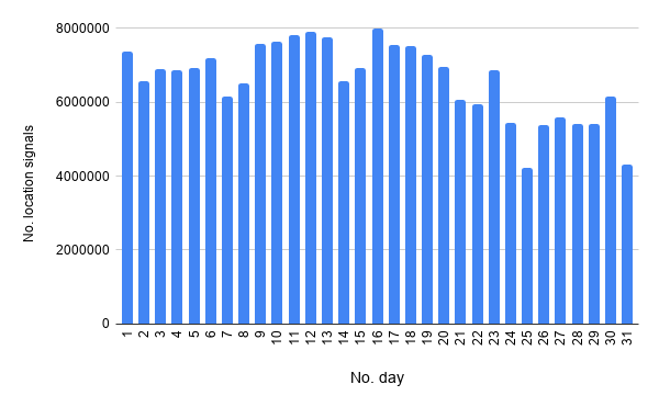
Figure 1. No. of location signals per Day in Manhattan in Dec 2019.

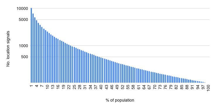
Figure 2. Distribution of location signals in Manhattan in Dec 2019.

2.1. Mobility Pattern

The mobility pattern determines where each agent is at each point in time during the simulation. We use real-world location signals provided by Veraset (ver, 2020). Veraset (ver, 2020) is a data-as-a-service company that provides anonymized population movement data collected through GPS signals of cell-phones across the US. We were provided access to this dataset for the months of December, January and (from 5th to 26th of) March. For a single day in December, there are 2,630,669,304 location signals across the US. Each location signal corresponds to a device_id and there are 28,264,106 device_ids across the US in that day. We assume each device_id corresponds to a unique individual . Fig. 2 shows the number of daily location signals recorded in the month of Dec. 2019 in the area of Manhattan, New York. Furthermore, Fig. 2 shows the distribution of location signals across individuals in Manhattan in Dec 2019. A point $(x,y)$ in Fig. 2 means that $x$ percent of the individuals have at least $y$ location signals in the month of Dec. in Manhattan. Using this real-world location data, we are able to create infection patterns for different cities and at different periods of time. This allows us to study the hypotheses that concern the spread of the disease for different cities and at different times.

Detailed statistics about the subset of the Veraset data we used for our experiments are discussed in Sec. 4. Here, we discuss our general approach of using real-world location signals for SpreadSim, independently of the actual dataset used. We consider a dataset such that each record in the dataset consists of an anonymized user_id, latitude, longitude and timestamp and is a location signal of the user with id user_id at the specified time and location. We consider each individual to be an agent in the simulation and for each agent, we have access to their latitude and longitude for various timestamps. Sorting this by time, we obtain a trajectory of location signals of an agent over time, denoted by the sequence $\langle c_{1},c_{2},...,c_{k}\rangle$. For two consecutive location signals, $c_{i}$ and $c_{i+1}$ of an agent at times $t_{i}$ and $t_{i+1}$, we assume the agent is at the location specified by $c_{i}$ from time $t_{i}$ to $t_{i+1}$. Using this interpolation, together with our location data, we have access to the location of every agent at every point in time during the simulation. We note that, although more sophisticated interpolations are possible, this falls beyond the scope of this paper, since our focus is on providing risk scores for different locations.

2.2. Transmission Model

Agents belong to either one of the following compartments: Susceptible (S), Infected and Not Spreading (INS), Infected and Spreading (IS) and Isolated or Recovered (R). An agent is said to be infected if they are in either INS or IS compartments. Intuitively, a susceptible agent can contract the disease, an INS agent is infected but cannot spread the disease, an IS agent is infected and can spread the disease and an Isolated or Recovered agent cannot spread the disease or contract it anymore. Figs. 4 and 4 illustrate the transmission model.

2.2.1. Compartments

All agents are initially Susceptible, with the exception of the agents that are infected initially as discussed in Sec. 2.3.1. We call the compartment an agent is in the agent’s status. Assume an agent gets infected at time $t$ based on the dynamics discussed in Sec. 2.2.2. Thus, at time $t$, the agent changes its status from Susceptible to Infected and Not Spreading. Consequently, at time $t+t_{IS}$, the agent becomes Infected and Spreading. Furthermore, at time $t+t_{R}$, the agent becomes Isolated or Recovered, where $t_{IS}\sim\mathcal{N}(\mu_{IS},\sigma_{IS})$ and $t_{R}\sim\mathcal{N}(\mu_{R},\sigma_{R})$, where $\mu_{IS},~{}\sigma_{IS},\mu_{R}$ and $\sigma_{R}$ are the parameters of the model. These parameters can be set based on existing research on COVID-19 (Ferretti et al., 2020; He et al., 2020; Li et al., 2020). For instance, (He et al., 2020) mentions that “ 1% of transmission would occur before 5 days and 9% of transmission would occur before 3 days prior to symptom onset”, while (Li et al., 2020) finds that incubation period (time from infection until onset of symptoms) has mean 5.2 days. Using this, we can find the parameter for the model that match the empirical evidence the best. We discuss the specific parameter setting used in our experiments in Sec. 4. We note that, first, $\mathcal{N}(\cdot)$ is a truncated normal distribution, such that if the sampled $t_{IS}$ or $t_{R}$ are less than zero, they are discarded and a new sample is obtained. Furthermore, if $t_{R}<t_{IS}$, the agent never spreads the disease, and moves directly from INS to the R compartment (the probability of either of these happening is very low based on the parameter setting chosen).

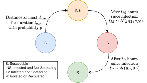
Figure 3. Transmission Model

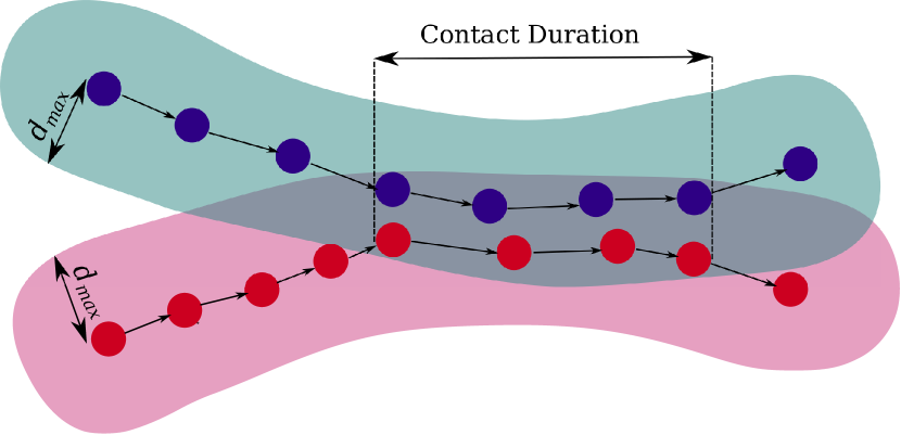
Figure 4. Transmission of disease through a co-location. Arrows show movement in time.

2.2.2. Transmission Dynamics

Only IS agents infect other agents, and only S agents get infected. Simply put, if an IS agent is within distance $d_{max}$ of an S agent for duration at least $t_{min}$ then, with probability $p$, the IS agent infects the S agent. $d_{max}$, $t_{min}$ and $p$ are the parameters of the transmission model. The model is designed to mimic how the disease spreads in the physical world, following the works of (Bromage, 2020; Wiersinga et al., 2020; Chu et al., 2020), where prolonged close-range contacts is the main source of transmission of the disease. Specifically, consider an IS agent, $u$, and an S agent $v$. At any time, $t$, during the simulation, consider the situation when the distance between $u$ and $v$ becomes at most $d_{max}$ (i.e., distance between $u$ and $v$ was larger than $d_{max}$ right before time $t$) from time $t$ until time at least $t+t_{min}$. Then, a number, uniformly at random, is generated in the range $[0,1]$. If the number is at most $p$, then $u$ infects $v$. When $v$ becomes infected, as explained in Sec. 2.2.1, its status changes from S to INS, and eventually to IS and R.

2.3. Initialization and Implementation

2.3.1. Initialization

. For a parameter $n_{init}$, we infect $n_{init}$ number of agents at the beginning of the simulation uniformly at random. The initial infections are treated as if the agent was infected by another agent. That is, an initially infected agent has initially the INS status and becomes IS after time $t_{IS}$ and recovered after $t_{R}$, where $t_{IS}$ and $t_{R}$ are sampled from the normal distributions discussed before.

2.3.2. Implementation

Our implementation SpreadSim first sorts all the location signals based on time. Subsequently, location signals are processed one by one in the order of time. Every location signal corresponds to an agent moving from an old location to a new location. As such, if the agent is susceptible, we check if there are any IS agents within $d_{max}$ of the new location. If the agent is IS, we check if there are any S agents within its $d_{max}$. We call it a co-location if an two agents are within $d_{max}$ distance of each other. Next, for any co-location between an S agent $u$ and an IS agent $v$, we check if it lasts for at least $t_{min}$. If it does, then, with probability $p$, we infect $u$. We use a grid to index the location of the agents. Given a new location signal at a new location, $(x,y)$, we perform a range search on the grid to find agents within $d_{max}$ of $(x,y)$. For each agent that matches the range search predicate, we then check if their co-location lasts for at least $t_{min}$. This can be optimized further by building a multidimensional index on both time and location.

3. Learning Spatiotemporal Risk Scores with LocationRisk@T

We now describe our Hawkes process model, LocationRisk@T, which leverages location data along with mobility patterns in a particular region to assign spatiotemporal risk scores. For a given city, we first form clusters $c\in\mathcal{C}$ using $k$-means clustering algorithm based on location signals in the city. The number of such clusters can be chosen according to the desired spatial resolution .

3.1. Mobility-aware Modelling

LocationRisk@T leverages the Origin-Destination (OD) matrix to represent the flow between two clusters $c$ and $c^{\prime}$ in a city. OD matrices are a popular way to encode spatial traffic flow information between two nodes in a transportation graph (Abrahamsson, 1998). Specifically, let $\mathcal{G}^{t}(V,E)$ denote a directed graph, where the edge weight $w_{i\rightarrow j}(t)$ encodes the traffic volume from cluster $i$ to $j$ between time $(t-1)$ and $t$. The OD matrix $W(t)\in\mathbb{R}^{|\mathcal{C}|\times|\mathcal{C}|}$ represents the traffic flows between different clusters $c\in\mathcal{C}$ in a city at time $t$. Here, the diagonal elements $w_{i\rightarrow i}(t)$ denote the traffic generated in a cluster $i$. We use this traffic flow information to inform LocationRisk@T.

We form the the mobility feature vector at time $t$, $\bm{m}_{\mathcal{G}_{c}}^{t}\in\mathbb{R}^{f}$, elements of which encode the different mobility features derived from the OD matrix $W$. Here, we develop two Hawkes process-based models a) LocationRisk@T_Mob, and b) LocationRisk@T${}_{Mob^{+}}$, depending upon the traffic flow features. For LocationRisk@T_Mob we set

(LocationRisk@T_Mob Features) $$\bm{m}_{c}^{t}=\begin{bmatrix}w_{c\rightarrow c}(t),~{}w_{to-c}(t),~{}w_{from-c}(t)\end{bmatrix}^{\top},$$

where

$$w_{to-c}(t):=\sum\limits_{c^{\prime}\in\mathcal{C}\backslash c}w_{c^{\prime}\rightarrow c}(t)\hskip 28.45274pt\text{and}\hskip 28.45274ptw_{from-c}(t):=\sum\limits_{c^{\prime}\in\mathcal{C}\backslash c}w_{c\rightarrow c^{\prime}}(t),$$

and $``\backslash^{\prime\prime}$ denotes the set difference operator. In effect, LocationRisk@T_Mob considers the net traffic to and from a clusters along with the location signals’ density, while being agnostic to the infections in each cluster.

To make the model infection-aware, we design LocationRisk@T${}_{Mob^{+}}$ which has additional mobility-based features to account for the infections at the origin cluster. Let $I_{c}(t)$ denote the infections in cluster $c$ at time $t$, and further let $I_{-c}(t)$ denote the total infections (over all clusters) except those in cluster $c$, i.e.,

$$I_{-c}(t)=\sum\limits_{c^{\prime}\in\mathcal{C}\backslash c}I_{c^{\prime}}(t).$$

We formulate the infection mobility to a cluster $c$ as

$$Im_{to-c}(t):=\dfrac{w_{to-c}(t)}{\sum\limits_{c^{\prime}\in\mathcal{C}\backslash c}\left(w_{to-c^{\prime}}(t)+w_{from-c^{\prime}}(t)\right)}\cdot I_{-c}(t).$$

Here, $Im_{to-c}(t)$ captures the proportion of infections travelling to a cluster $c$. Similarly, we also form $Im_{of-c}(t)$ to weigh the total number of infections in a cluster $c$ by the ratio of self-mobility and traffic from other clusters.

$$Im_{of-c}(t):=\dfrac{w_{c\rightarrow c}(t)}{w_{to-c}(t)}\cdot I_{c}(t).$$

With these features, we form the feature set for LocationRisk@T${}_{Mob^{+}}$ as follows.

(LocationRisk@T$${}_{Mob^{+}} \bm{m}_{c}^{t}=\begin{bmatrix}w_{c\rightarrow c}(t),~{}w_{to-c}(t),~{}w_{from-c}(t),~{}Im_{to-c}(t),~{}Im_{of-c}(t)\end{bmatrix}^{\top}$$ Features)

3.2. Incorporating Mobility Features into Hawkes Process

Now, given the daily infections at each cluster $c\in\mathcal{C}$, i.e. a realization of a point process $N_{c}(t)$ on $[0,T]$ for $T<\infty$, at timestamps $\mathcal{T}_{c}=\{t_{1}^{c},t_{2}^{c},\dots t_{n}^{c}\}$, we model the rate of new cases at time $t$, $\lambda_{c}(t)$ associated with a cluster $c$ by incorporating the corresponding traffic mobility features $\bm{m}_{c}^{t}$ developed in Sec. 3.1 as

(1) $$\lambda_{c}(t)=\mu_{c}+\sum_{t>t_{j},t_{j}\in\mathcal{T}}R_{c}^{t_{j}}(\bm{m}_{c}^{t_{j}-\Delta},\theta)~{}wbl(t_{i}-t_{j}),$$

where, $\mu_{c}$ is known as the background rate, and captures the inherent proclivity of a cluster to produce infections. We use Weibull distribution, $wbl(\cdot)$ with shape $\alpha$ and scale $\beta$ to model the inter-event time, which specifies the influence of past events. The time-delay parameter $\Delta$ is used to account for the delay between the mobility and the infections.

The mobility features are used to model the time-varying cluster-dependent reproduction number $R_{c}^{t}(\bm{m}_{c}^{t-\Delta},\theta)$. In particular, we model the dynamic reproduction number $R_{c}^{t}$ as a Poisson regression task (Chiang et al., 2020), including the traffic-flow based mobility features for each cluster as

(2) $$\bm{E}_{R}[R_{c}^{t_{j}}|\bm{m}_{c}^{t_{j}-\Delta},\theta]=\exp(\theta^{\top}\bm{m}_{c}^{t_{j}-\Delta}),$$

where $\bm{E}[\cdot]$ denotes the expectation operator.

The mobility and cluster-dependent reproduction number $R_{c}^{t}(\bm{m}_{c}^{t-\Delta},\theta)$ can be viewed as the average number of secondary infections caused by a primary infection (in the Granger sense (Granger, 1969; Eichler et al., 2017; Yuan et al., 2019)). In addition, the first term $\mu_{c}$ helps in modelling the effect of factors not captured by the mobility-dependent second term.

Overall, LocationRisk@T incorporates the actual high-resolution mobility patterns within a city, which enables us to learn informative spatiotemporal risk scores (developed in Sec. 3.4). As compared to related mobility-based methods (such as (Chiang et al., 2020)) which rely only on mobility density, LocationRisk@T leverage fine-grained flow information. The main task now is to infer the model parameters $\theta$ of LocationRisk@T using the mobility features and the infections. We now describe the Expectation Maximization-based inference procedure to learn $\theta$.

3.3. Expectation Maximization-based Inference Procedure

We adopt an Expectation Maximization-based approach to infer the parameters $\theta$. Our algorithm (outlined in Algorithm 1) provides an iterative way to evaluate the maximum-likelihood estimates of LocationRisk@T. We begin by introducing latent variables $Y$ in order to model the unobserved variables of our model. To this end, we begin by writing the likelihood $\mathcal{L}(\Theta;X)$ for Hawkes process given data $X=\left(\{t_{j}^{c}\}_{j=1,c=1}^{|\mathcal{T}_{c}|,|\mathcal{C}|},\{\bm{m}_{c}^{t}\}_{c=1,t=1}^{|\mathcal{C}|,|\mathcal{T}|}\right)$ and model parameters $\Theta=\left(\{\mu_{c}\}_{c=1}^{\mathcal{C}},\theta\right)$ as

(3) $$\mathcal{L}(\Theta;X)=\prod_{c=1}^{|\mathcal{C}|}\prod_{i=1}^{n}\lambda_{c}(t_{i})\exp^{-\int_{0}^{T}\lambda_{c}(t)dt}.$$

For the EM procedure, we introduce latent variables $Y^{c}_{ij}$ to indicate that an event $j$ is an off-spring event $i$ in cluster $c$, and $Y_{ii}^{c}$ to denote that it was generated by a background event (in $c$), to formulate the complete data log-likelihood as

(4) $$\log(\mathcal{L}(\Theta;X,Y))=\sum_{c=1}^{|\mathcal{C}|}\sum_{i=1}^{n}Y^{c}_{ii}\log(\mu_{c})+Y^{c}_{ij}\log\left(\sum_{t_{i}>t_{j},t_{j}\in\mathcal{T}}R_{c}^{t_{j}}(\bm{m}_{c}^{t_{j}-\Delta},\theta)~{}wbl(t-t_{j})\right)-\int_{0}^{T}\lambda_{c}(t)dt.$$

Algorithm 1 LocationRisk@T: Mobility-based Hawkes process Model using Poisson Regression

Input: The timestamps set $\mathcal{T}_{c}=\{t_{j}^{c}\}_{j=1}^{|\mathcal{T}|}$for each cluster $c\in\mathcal{C}$(e.g. daily infections in each cluster within a city). Daily Origin-Destination matrix $\{W(t)\}\}_{t=0}^{T}$consisting of mobility patterns within a city to form mobility features $\{\bm{m}_{c}^{t}\}_{c=1,t=0}^{|\mathcal{C}|,|\mathcal{T}|}$. Weibull shape and scale parameters $\alpha$and $\beta$, time delay parameter $\Delta$, and the tolerance parameter $\delta$.

Output: Estimates $\theta$ and $\{\mu_{c}\}_{c=1}^{\mathcal{C}}$.

Initialize: $\mu_{c}\leftarrow 0.5$ for all $c\in\mathcal{C}$, $R_{c}^{t}\leftarrow 1$ for all $c\in\mathcal{C}$ and $t\in\mathcal{T}$, $T\leftarrow\max\mathcal{T}$, and $k=1$.

while $\|\Delta\theta\|\geq\delta$ and $\|\Delta\mu_{c}\|\geq\delta$ for all $c\in\mathcal{C}$ do

Expectation Step:

      for $\forall~{}i\geq j$ and $0<i$, $j<T$ and $\forall~{}c\in\mathcal{C}$ do

             if i¿j then

                   $p_{c}(i,j)=\dfrac{R_{c}^{t_{j}}(\bm{m}_{c}^{t_{j}-\Delta},\theta)~{}wbl(t-t_{j})}{\lambda_{c}(t_{i})}$

            else if  i = j  then

                   $p_{c}(i,i)=\dfrac{\mu_{c}}{\lambda_{c}(t_{i})}$

            

       end for

Maximization Step:

Update $\theta$: $\hat{\theta}\leftarrow\underset{\theta}{\arg\max}\sum_{c=1}^{|\mathcal{C}|}\left(\sum_{j=1}^{n}P_{c}(j)\theta^{\top}\bm{m}_{c}^{t_{j}-\Delta}-\exp(\theta^{\top}\bm{m}_{c}^{t_{j}-\Delta})\right)$

Update $\mu_{c}$s: $\hat{\mu_{c}}\leftarrow\sum_{i=1}^{n}\tfrac{p_{c}(i,i)}{T}$ for all $c\in\mathcal{C}$.

$k\leftarrow k+1$

      

end while

3.3.1. Expectation Step

Since both $\log(\mathcal{L}(\Theta;X,Y))$ and $Y$ are random variables, at the $k$-th iteration in the E-step we evaluate the expectation function $Q(\Theta,\Theta^{k-1})$ as

(5) $$Q(\Theta,\Theta^{k-1}) =\bm{E}_{Y}[\log(\mathcal{L}(\Theta;X,Y))|X,\Theta^{k-1}],$$

$$=\int\log(\mathcal{L}(\Theta;X,Y))f(Y|X,\Theta^{k-1})dY,$$

where $\Theta^{k-1}$ are the estimated parameters at the $(k-1)$-th iteration, and $f(Y|X,\Theta^{k-1})$ is the conditional distribution of $Y$ given $X$ and $\Theta^{k-1}$. Specifically, as in (Chiang et al., 2020), we estimate the probability $p_{c}(i,j)$ as follows

$$p_{c}(i,j):=\bm{E}_{Y}[Y^{c}_{ij}|X,\Theta^{k-1}]=\dfrac{R_{c}^{t_{j}}(\bm{m}_{c}^{t_{j}-\Delta},\theta)~{}wbl(t-t_{j}|\alpha,\beta)}{\lambda_{c}(t_{i})}$$

and $p_{c}(i,i)$ as

$$p_{c}(i,i):=\bm{E}_{Y}[Y^{c}_{ii}|X,\Theta^{k-1}]=\dfrac{\mu_{c}}{\lambda_{c}(t_{i})}.$$

3.3.2. Maximization Step

Based on the probabilities $p_{c}(i,j)$ and $p_{c}(i,i)$, we estimate the parameters by maximizing $Q(\Theta,\Theta^{k-1})$ in (5) w.r.t. to each parameter. With this, we arrive at the following update steps for each parameter (Chiang et al., 2020). Specifically, we learn the parameters $\theta$ via Poisson regression as

$$\hat{\theta}:=\underset{\theta}{\arg\max}\sum_{c=1}^{|\mathcal{C}|}\left(\sum_{j=1}^{n}P_{c}(j)\theta^{\top}\bm{m}_{c}^{t_{j}-\Delta}-\exp(\theta^{\top}\bm{m}_{c}^{t_{j}-\Delta})\right),$$

where $P_{c}(j)=\sum_{i=j+1}^{n}p_{c}(i,j)$, and the following closed form update for the background rate parameters:

$$\hat{\mu_{c}}:=\underset{\mu_{c}}{\arg\max}\sum_{i=1}^{n}p_{c}(i,i)\log(\mu_{c})-\int_{0}^{T}\mu_{c}dt=\sum_{i=1}^{n}\tfrac{p_{c}(i,i)}{T}.$$

3.4. Characterizing Risk

The dynamic reproduction number (commonly referred to as $R0$) has been used to assign risk scores to communities (Kiamari et al., 2020). Indeed as explored by (Chiang et al., 2020), the reproduction number is dependent on the mobility density over time. However, since the reproduction number is highly sensitive to parameter choices and models (Delamater et al., 2019; Li et al., 2011), LocationRisk@T leverages both the dynamic reproduction number $R_{c}^{t}$ and the background rate $\mu_{c}$ associated with a cluster $c$ to assign risk scores. Specifically, we propose a spatiotemporal risk score based on the intensity function $\lambda_{c}(t)$ of LocationRisk@T. Let $\Lambda\in\mathbb{R}^{|\mathcal{C}|\times T}$ be a matrix where $\Lambda(c,t)=\lambda_{c}(t)$. Then, we define our risk score $\rho\in[0,1]$ for a cluster $c$ at time $t$ as

(6) $$Risk~{}Score~{}\rho_{c}(t)=\dfrac{\lambda_{c}(t)-\underset{c^{\prime}\in\mathcal{C},t^{\prime}\in T}{\min}~{}\Lambda(c^{\prime},t^{\prime})}{\underset{c^{\prime}\in\mathcal{C},t^{\prime}\in T}{\max}~{}\Lambda(c^{\prime},t^{\prime})-\underset{c^{\prime}\in\mathcal{C},t^{\prime}\in T}{\min}~{}\Lambda(c^{\prime},t^{\prime})}.$$

This essentially scales the intensity function of the disease relative to the intensities in other clusters over time, and alleviates the issues associated with calculating accurate reproduction number.

City	December	January	March
San Francisco	116$\times 10^{6}$	96$\times 10^{6}$	61$\times 10^{6}$
Miami	75$\times 10^{6}$	105$\times 10^{6}$	64$\times 10^{6}$
Chicago	135$\times 10^{6}$	175$\times 10^{6}$	107$\times 10^{6}$
Houston	135$\times 10^{6}$	182$\times 10^{6}$	105$\times 10^{6}$

Table 1. Total No. location signals per Month

City	December	January	March
San Francisco	62$\times 10^{3}$	72$\times 10^{3}$	55$\times 10^{3}$
Miami	42$\times 10^{3}$	55$\times 10^{3}$	46$\times 10^{3}$
Chicago	76$\times 10^{3}$	106$\times 10^{3}$	90$\times 10^{3}$
Houston	69$\times 10^{3}$	97$\times 10^{3}$	78$\times 10^{3}$

Table 2. No. Agents per Month

Parameter	Description	Value
$d_{max}$	Maximum distance for a co-location	$\sim 11m$
$t_{min}$	Minimum duration for infection	$1h$
$p$	Probability of infection	1
$n_{init}$	Number of agents initially infected	1,000
$\mu_{IS}$	Average number of days for an agent to become IS from infection	5
$\sigma_{IS}$	Std. deviation of number of days for an agent to become IS from infection	1
$\mu_{R}$	Average number of days for an agent to become R from infection	12
$\sigma_{R}$	Std. deviation of number of days for an agent to become R from infection	2.4

Table 3. SpreadSim Parameter Setting

4. Experimental Results

We now evaluate and compare the performance of our proposed method with competing techniques based on the accuracy of their infection and risk prediction over different months and cities in the United States (US).

4.1. Data

The statistics of our dataset is summarised in Tables 2 and 2. We obtained the data from Veraset (ver, 2020) a data-as-a-service company that provides anonymized population movement data collected through GPS signals of cell-phones across the US. The obtained dataset consists of location signals across the US for the time-periods December 1, 2019 to January 31, 2020, as well as March 5, 2020 to March 26, 2020. For each of the cities or counties considered, we first use a range defined by a rectangle that roughly covers the area of the city or county to select the location signals that fall within the area. Each record in the dataset consists of anonymized_device_id, latitude, longitude, timestamp and horizontal accuracy. We assume each anonymized_device_id corresponds to a unique individual. We discard any location signal with horizontal accuracy of worse than 25 meters. Furthermore, we filter out individuals with less than 100 location signals for every one-month period considered.

	Day $10$	Day $15$	Day $20$
Dec. ‘19
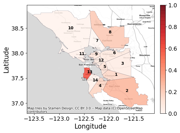
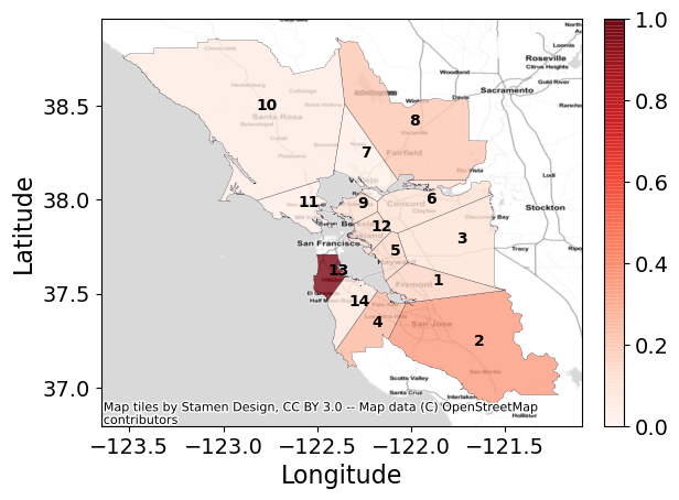
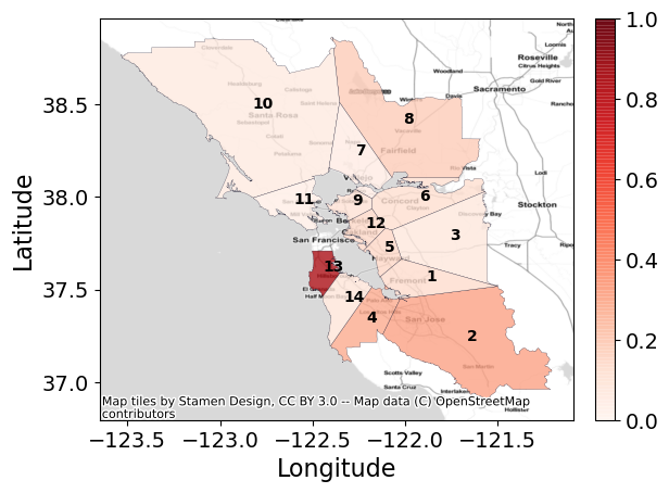
	(a-i)	(a-ii)	(a-iii)
Jan. ‘20
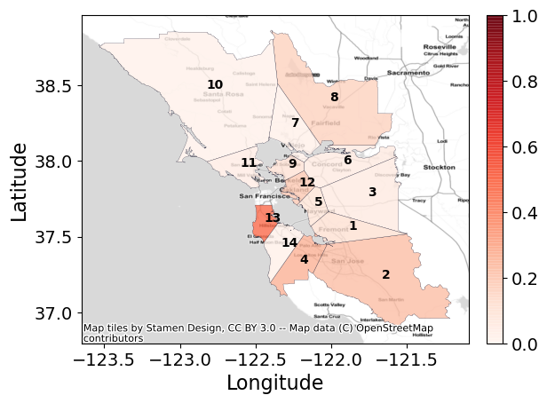
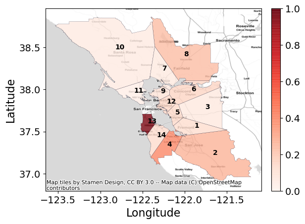
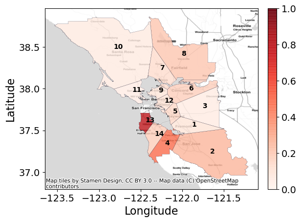
	(b-i)	(b-ii)	(b-iii)
Mar. ‘20
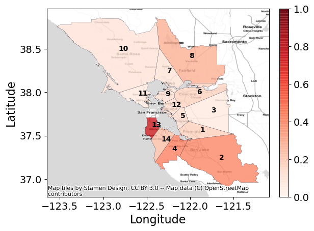
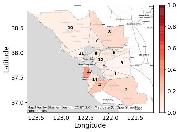
	(c-i)	(c-ii)	(c-iii)
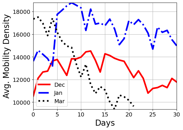
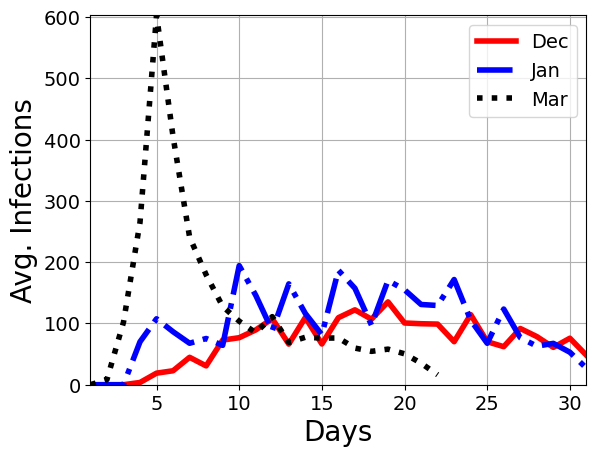
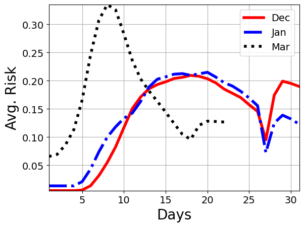
	(d-i)	(d-ii)	(d-iii)

Figure 5. Comparing the Risk across months in different regions of San Francisco–Bay Area, CA. Panels (a), (b), and (c) show the evaluated risk ($\rho$) for each cluster (marked via numbers) for the months of Dec ‘19, Jan ‘20, and Mar ‘20, respectively. The panels (i), (ii), and (iii) show the risk varying over day 10, 15, and 20, respectively. In addition, panel (d-i), (d-ii), and (d-iii) show the comparison between the average number of location signals, infections and risk, across clusters over months, respectively. We observe that while the risk for months of Dec and Jan show similar trends for different days, the month of Mar has lower risk later in the month, which can be attributed to the drop in mobility; see cluster $12$ (best viewed digitally).

Model	Infection and Risk Prediction for San Francisco–Bay Area, CA
	December ‘19				January ‘20				March ‘20
	$(\alpha,\beta,\Delta)=(2,2,3)$				$(\alpha,\beta,\Delta)=(2,2,12)$				$(\alpha,\beta,\Delta)=(2,2,12)$
	R-MAE(I)	$\sigma$(I)	MAE($\rho_{\mathrm{test}}$)	MAE($\rho_{\mathrm{all}}$)	R-MAE(I)	$\sigma$(I)	MAE($\rho_{\mathrm{test}})$	MAE($\rho_{\mathrm{all}}$)	R-MAE(I)	$\sigma$(I)	MAE($\rho_{\mathrm{test}}$)	MAE($\rho_{\mathrm{all}}$)
HawkesDen	0.272	0.138	0.073	0.037	0.615	0.162	0.117	0.048	1.284	0.197	0.168	0.139
LocationRisk@TMob	0.224	0.131	0.313	0.257	0.340	0.139	0.067	0.038	0.758	0.157	0.169	0.142
LocationRisk@T${}_{Mob^{+}}$	0.136	0.115	0.091	0.046	0.140	0.123	0.045	0.040	0.281	0.126	0.101	0.112

Table 4. Predicting (5-day) Infections and Risk for San Francisco–Bay Area, CA. The table shows the error in predicted infections (I), the corresponding standard deviation, risk ($\rho$) for the test set, and over all days for Dec ‘19, Jan ‘20, and Mar ‘20 for the top-$5$ clusters.

4.2. Experimental Setup

We run SpreadSim described in Sec. 2 for the areas around the cities of San Francisco (and the bay area), Miami (Miami-Dade county), Chicago (Cook county) and Houston (Harris county) over the available days in December 2019, January 2020, and March 2020. The results for more cities across the US can be found in Appendix A. For each city and month, SpreadSim starts on day 1 and ends on the last day of the month, generating a disease spread pattern based on activities of the agents. For each experiment, we use the last $5$ days as our test set to evaluate LocationRisk@T’s infection and risk prediction performance.

4.2.1. SpreadSim Parameters

For SpreadSim, the parameter setting is shown in Table 3. We set $\mu_{IS}$ to 5 similar to the mean incubation period reported in (Li et al., 2020), and $\sigma_{IS}=1$ since (He et al., 2020) observed that most infections occur within 3 days of symptom onset. The work in (He et al., 2020) reports “Infectiousness was estimated to decline quickly within 7 days”, so we set $\mu_{R}$ to $\mu_{IS}+7$. We use a larger value for $\sigma_{R}$ to account for the fact that some people may self-isolate after the onset of the symptoms. We use a value for $d_{max}$ larger than the common 2 meter (m) recommendation for social distancing as the discussion in (Bromage, 2020) shows how infections can happen through co-locations with a larger separation between individuals if the co-location lasts for a long enough duration. Thus, we also set $t_{min}$ to 1 hour, larger than the 15 minute minimum threshold mentioned by (Wiersinga et al., 2020). Moreover, because we consider co-locations that are at least 1h, we set $p=1$, as the probability of infection becomes higher when co-locations last for long periods.

Furthermore, note that the accuracy of our location data is to about 25m, which is larger than the value we used for $d_{max}$. Thus, the inaccuracy in our location data can affect who gets infected in the simulation. However, this does not impact the quality of the infection patterns generated, because the 25m accuracy still ensures that an agent in the same area as the infected agent will get infected. For instance, if an infected person is in a shopping mall, the other infected agents will still be in the shopping mall.

Finally, we note that although we have made every effort to design SpreadSim such that it follows the transmission dynamics of COVID-19, existing inaccuracies in the transmission model do not affect the observations made in this paper. This is because, firstly, SpreadSim is used to generate the ground-truth. The models predicting risk-scores are both trained and evaluated against on this ground-truth data. Secondly, SpreadSim is used consistently across all the baselines and our proposed models, and thus our evaluation is fair.

4.2.2. Baselines

We analyze the performance of LocationRisk@T_Mob and LocationRisk@T${}_{Mob^{+}}$ – the two variants which utilize the fine-grain mobility-flow information (as described in Sec. 3.1) along with Hawkes_Den, which relies only on the mobility density in the clusters and is the state-of-the-art approach for spatiotemporal modeling of COVID-19 from mobility data (Chiang et al., 2020). Specifically, Hawkes_Den uses the location signals at the clusters, with the mobility density feature defined as

(Hawkes_Den Features) $$\bm{m}_{c}^{t}=\begin{bmatrix}w_{c\rightarrow c}(t)\end{bmatrix}.$$

Model	Infection and Risk Prediction for Miami, FL
	December ‘19				January ‘20				March ‘20
	$(\alpha,\beta,\Delta)=(2,2,12)$				$(\alpha,\beta,\Delta)=(2,2,18)$				$(\alpha,\beta,\Delta)=(2,2,12)$
	R-MAE(I)	$\sigma$(I)	MAE($\rho_{\mathrm{test}}$)	MAE($\rho_{\mathrm{all}}$)	R-MAE(I)	$\sigma$(I)	MAE($\rho_{\mathrm{test}})$	MAE($\rho_{\mathrm{all}}$)	R-MAE(I)	$\sigma$(I)	MAE($\rho_{\mathrm{test}}$)	MAE($\rho_{\mathrm{all}}$)
HawkesDen	0.383	0.189	0.121	0.058	1.216	0.285	0.102	0.075	1.365	0.227	0.244	0.154
LocationRisk@TMob	0.162	0.164	0.087	0.043	0.196	0.178	0.064	0.076	1.229	0.219	0.235	0.147
LocationRisk@T${}_{Mob^{+}}$	0.092	0.146	0.064	0.040	0.152	0.163	0.031	0.054	0.308	0.128	0.117	0.110

Table 5. Predicting (5-day) Infections and Risk for Miami, FL. The table shows the error in predicted infections (I), the corresponding standard deviation, risk ($\rho$) for the test set, and over all days for Dec ‘19, Jan ‘20, and Mar ‘20 for the top-$5$ clusters.

4.2.3. Metrics

We evaluate the techniques on two main criteria – a) infection prediction, to judge the model fit, and b) risk prediction to analyze the efficacy of using the proposed risk metric in Eq. (6) as a reliable indicator for predicting potential risk associated with a region over time. For infection prediction we use mean relative absolute error (relative-MAE) between the predicted infection trajectory and the true infections (R-MAE(I)) as the performance metric. This relative measure accounts for the scale differences (in number of infections) across different clusters. In addition, we also report the standard deviation of the predicted infection trajectory ($\sigma$(I)) corresponding to our relative-MAE metric. For risk prediction, we report the mean absolute error (MAE) between the the predicted risk and the infections (scaled between 0 and 1) on the test set (MAE($\rho_{\mathrm{test}}$)) and overall (MAE($\rho_{\mathrm{all}}$)).

	Day $10$	Day $15$	Day $20$
Dec. ‘19
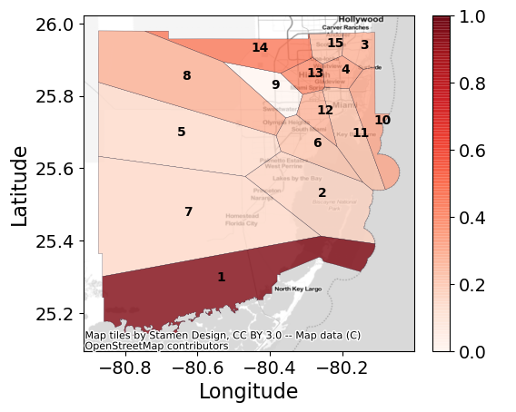
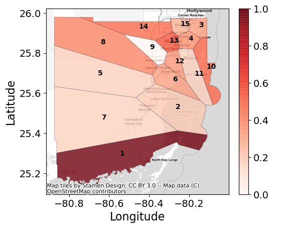
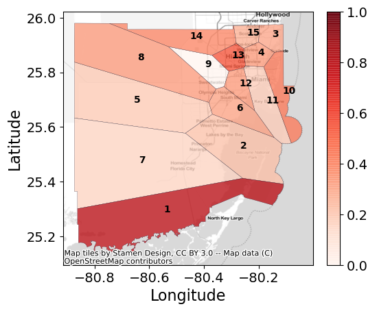
	(a-i)	(a-ii)	(a-iii)
Jan. ‘20
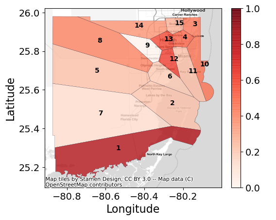
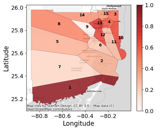
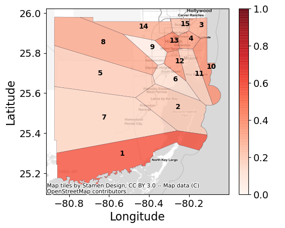
	(b-i)	(b-ii)	(b-iii)
Mar. ‘20
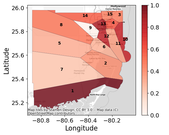
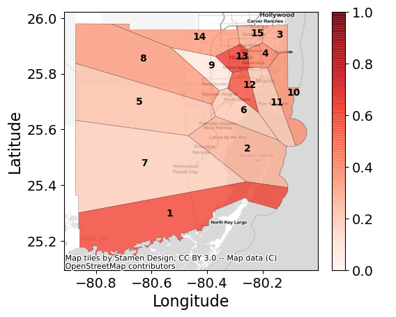
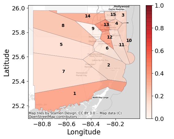
	(c-i)	(c-ii)	(c-iii)
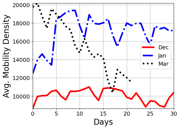
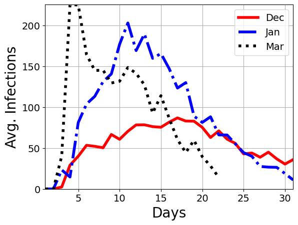
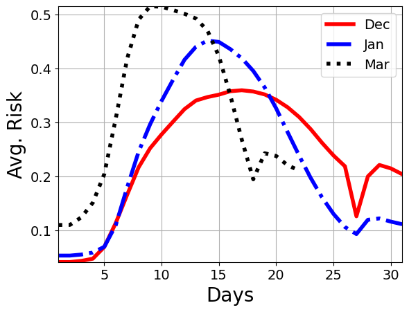
	(d-i)	(d-ii)	(d-iii)

Figure 6. Comparing the Risk across months in different regions of Miami, FL. Panels (a), (b), and (c) show the evaluated risk ($\rho$) for each cluster (marked via numbers) for the months of Dec ‘19, Jan ‘20, and Mar ‘20, respectively. The panels (i), (ii), and (iii) show the risk varying over day 10, 15, and 20, respectively. In addition, panel (d-i), (d-ii), and (d-iii) show the comparison between the average number of location signals, infections and risk, across clusters over months, respectively. We observe that while the risk for months of Dec and Jan show similar trends for different days, the month of Mar has lower risk later in the month, which can be attributed to the drop in mobility; see cluster $1$ (best viewed digitally).

4.2.4. Pre-processing steps

We use Origin-Destination (OD) matrix $W(t)$ as a means to gauge the traffic-flow characteristics on day $t$. The OD matrix is a $|\mathcal{C}|\times|\mathcal{C}|$ matrix where $|\mathcal{C}|$ is the number of clusters. In our experiments we set $|\mathcal{C}|=15$. The entry $w_{i\rightarrow j}(t)$ on the $i$-th row and the $j$-th column of $W(t)$ is calculated as the total count of consecutive location signals, $\mathscr{c}$ and $\mathscr{c}^{\prime}$, over all individuals, such that $\mathscr{c}$ is in cluster $i$ and $\mathscr{c}^{\prime}$ is in cluster $j$; see also Sec. 3.1.

Next, we use a 6-day moving median filter to smooth the infection and mobility traces. Empirically, we find that such a smoothing helps to counter the dominance of a cluster with sudden rise in cases on the learned model. All mobility features are standardized, meaning that we subtract the mean and divide by the standard deviation.

4.2.5. Parameter Choices

The main parameters of the model are the Weibull parameters ($\alpha$, $\beta$) and the time delay parameter $\Delta$. For each city and month, we choose set of parameters ($\alpha$, $\beta$, $\Delta$) which yields the best relative-MAE on infection prediction. For a fair comparison, all techniques are provided with the same set of parameters for a city and month.

4.3. Results

We show the infection prediction performance measured in terms of R-MAE and the risk prediction performance in terms of the MAE between the evaluated risk and scaled infections for top-$5$ clusters (in terms of location signals) of the metropolitan areas of San Francisco, Miami, Chicago and Houston in Tables 4, 5, 6, and 7, respectively. We provide additional results for the metro areas of Los Angeles, New York, Seattle, and Salt lake County in Appendix A. For each of these cities, LocationRisk@T${}_{Mob^{+}}$ yields the best infection prediction performance across all months considered. Furthermore, our models LocationRisk@T_Mob and LocationRisk@T${}_{Mob^{+}}$ are also more robust ($\rho_{\mathrm{test}}$ performance) and yield superior performance overall for risk prediction as compared to the density-only baseline of Hawkes_Den. Note that like any learning model, the prediction capabilities are sensitive to the amount of available infections. As a result, the prediction accuracy for clusters with small number of infections is not high. Arguably, the risk scores for clusters with large number of infections matter more, and for low-infection levels contact tracing may be a more effective tool.

Model	Infection and Risk Prediction for Chicago (Cook County), IL
	December ‘19				January ‘20				March ‘20
	$(\alpha,\beta,\Delta)=(2,2,7)$				$(\alpha,\beta,\Delta)=(2,2,9)$				$(\alpha,\beta,\Delta)=(2,2,9)$
	R-MAE(I)	$\sigma$(I)	MAE($\rho_{\mathrm{test}}$)	MAE($\rho_{\mathrm{all}}$)	R-MAE(I)	$\sigma$(I)	MAE($\rho_{\mathrm{test}})$	MAE($\rho_{\mathrm{all}}$)	R-MAE(I)	$\sigma$(I)	MAE($\rho_{\mathrm{test}}$)	MAE($\rho_{\mathrm{all}}$)
HawkesDen	0.536	0.165	0.080	0.041	0.941	0.177	0.075	0.048	1.005	0.142	0.215	0.143
LocationRisk@TMob	0.337	0.151	0.071	0.038	0.238	0.129	0.037	0.053	0.342	0.098	0.173	0.144
LocationRisk@T${}_{Mob^{+}}$	0.162	0.126	0.053	0.035	0.174	0.118	0.045	0.071	0.209	0.083	0.071	0.078

Table 6. Predicting (5-day) Infections and Risk for Chicago (Cook County), IL. The table shows the error in predicted infections (I), the corresponding standard deviation, risk ($\rho$) for the test set, and over all days for Dec ‘19, Jan ‘20, and Mar ‘20 for the top-$5$ clusters.

	Day $10$	Day $15$	Day $20$
Dec. ‘19
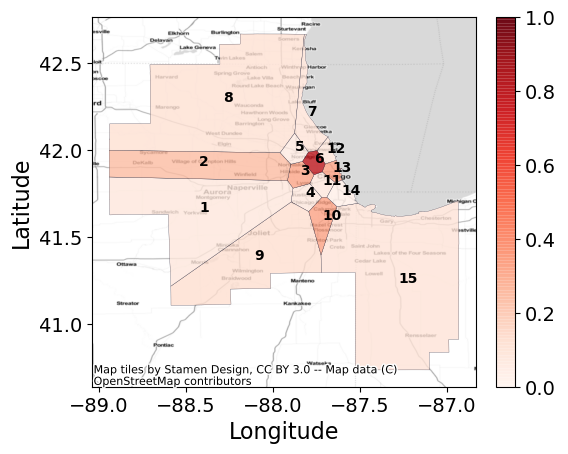
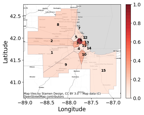
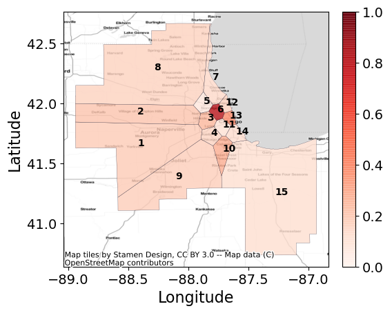
	(a-i)	(a-ii)	(a-iii)
Jan. ‘20
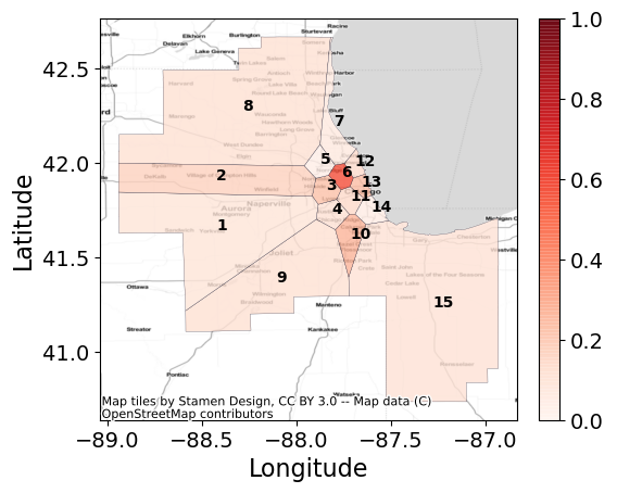
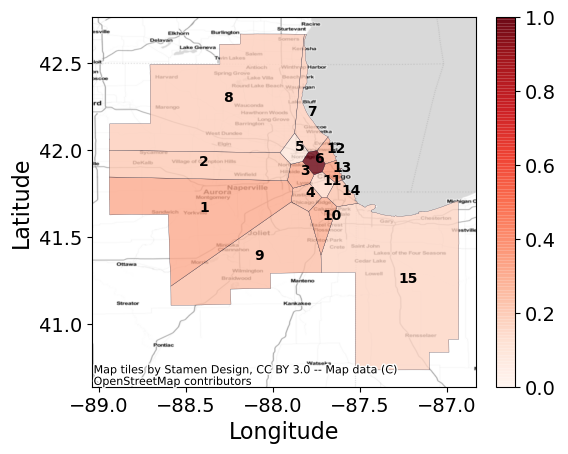
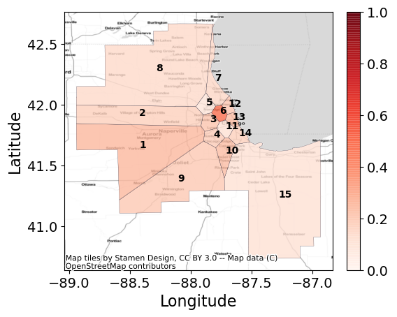
	(b-i)	(b-ii)	(b-iii)
Mar. ‘20
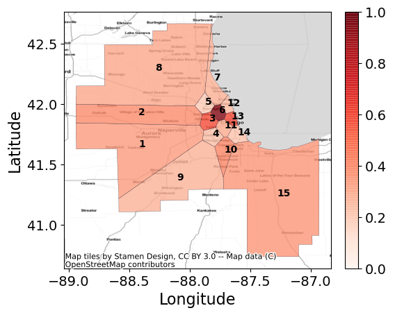
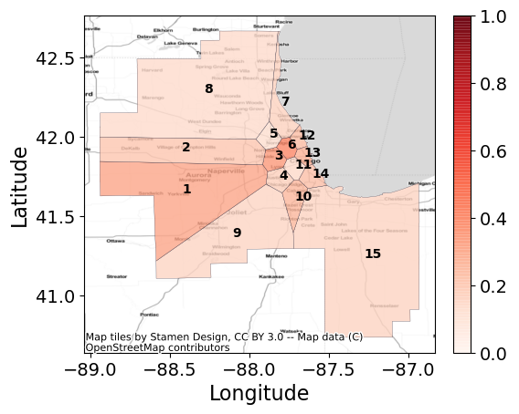
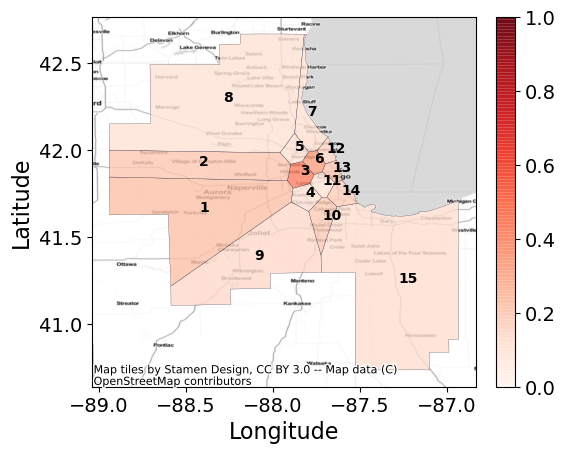
	(c-i)	(c-ii)	(c-iii)
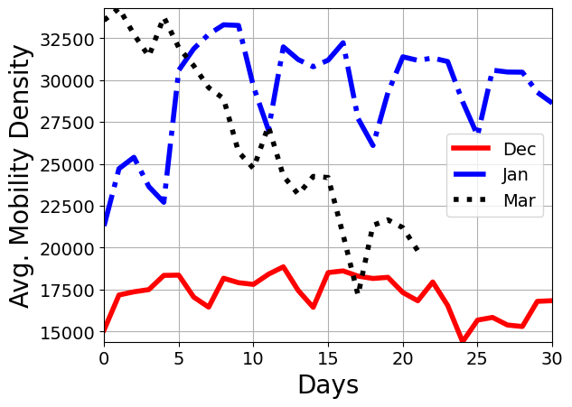
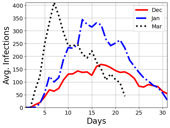
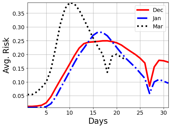
	(d-i)	(d-ii)	(d-iii)

Figure 7. Comparing the Risk across months in different regions of Chicago (Cook county), IL. Panels (a), (b), and (c) show the evaluated risk ($\rho$) for each cluster (marked via numbers) for the months of Dec ‘19, Jan ‘20, and Mar ‘20, respectively. The panels (i), (ii), and (iii) show the risk varying over day 10, 15, and 20, respectively. In addition, panel (d-i), (d-ii), and (d-iii) show the comparison between the average number of location signals, infections and risk, across clusters over months, respectively. We observe that while the risk for months of Dec and Jan show similar trends for different days, the month of Mar has lower risk later on, which can be attributed to the drop in mobility; see cluster $6$ (best viewed digitally).

In addition, in Figs. 5 6, 7, and 8 panels (a-c)(i-iii) we provide visualizations of the predicted spatiotemporal risk by LocationRisk@T${}_{Mob^{+}}$ corresponding to Tables 4, 5, 6, and 7, respectively, for day $10$, $15$, and $20$ of the months of Dec. 2019, Jan. 2020, and Mar. 2020. Furthermore, in panel (d) (i-iii) in each of these figures, we compare the corresponding average mobility density, infections and the predicted risk across all clusters (in a city) for these months. Note that here the risk scores are scaled from $[0,1]$ for each month, where a darker color represents a higher risk score relative to the risk in that month. From Figs. 5 6, 7, and 8 we note an interesting trend that the similar mobility patterns of the months of Dec. 2019 and Jan. 2020 (except for scale), leads to similar disease spread patterns, and ultimately similar risk scores. The month of Mar. 2020, however, is different for each of these cities from Dec. 2019 and Jan. 2020 across the board. Recall that the stay-at-home order was implemented in the middle of the Mar. 2020 (sta, 2020), hence our March dataset includes mobility patterns before, during and after the lock-down. Consequently, we observe higher mobility density during the beginning of the month (which results in higher infections early on). However, as the mobility drops (panel (d-i), there is a corresponding drop in the infections (panel (d-ii), and the risk scores by LocationRisk@T${}_{Mob^{+}}$ (panel (d-iii)). Here, LocationRisk@T${}_{Mob^{+}}$’s risk scores track the infections, emerging as a reliable spatiotemporal risk metric.

Lastly, another important observation is regarding the high-risk areas for each city. Our results using LocationRisk@T${}_{Mob^{+}}$ corroborates our intuition that popular destinations in a city are riskier. For instance, for the metro area of San Francisco, the actual downtown area turns out to be high-risk. This trend can also be observed in other cities as well. Here, the superior performance of LocationRisk@T${}_{Mob^{+}}$ over Hawkes_Den and LocationRisk@T_Mob for both infection and risk prediction can be attributed to modeling the infection mobility in addition to the location signal density and mobility. Incorporating the infection mobility as opposed to just relying on popularity of an area, as in case of Hawkes_Den, allows LocationRisk@T${}_{Mob^{+}}$ to improve infection prediction performance by being cognizant of the past infections in different areas in a city. As a result, LocationRisk@T${}_{Mob^{+}}$ underscores the importance of bringing together mobility patterns and infection spread prediction model to assign high-resolution risk scores.

5. Related Work

5.1. Disease Prediction and Mobility Indicators

Most popular disease prediction models employ compartmental models since they allow explicit modeling of the transmission characteristics. These mainly include variants of the classical Susceptible-Infected-Removed (SIR) model (Kermack and McKendrick, 1927), such as the S-Exposed-IR (SEIR) model and its variants, which primarily aim to add additional latent states to the SIR model (Miller et al., 2020). Popular in practice due to their simplicity, these models rely on the homogeneous population mixing to learn the model parameters, and have been used to predict reproduction number (R0) at coarser granularity for counties, states and entire countries (Bertozzi et al., 2020). Although useful to communicate the disease characteristics at early stages, coarse-grain risk scores and reproduction number estimates at county or state level are not readily usable for public policy decisions at finer spatial and temporal scales (Chande et al., 2020; Institute, 2020). On the other hand, Hawkes process-based point process disease spread models have also emerged as an alternative way to model COVID-19 spread (Chiang et al., 2020). Even though mathematical similarities between compartmental models and Hawkes process-based models exist, Hawkes process-based modeling does not involve complex parameter estimation, model identifiability and mis-specification as in the case of SEIR model (Kresin et al., 2020; Evans et al., 2005; Roosa and Chowell, 2019; Hengartner and Fenimore, 2018; Osthus et al., 2017).

Moving away from homogeneous mixing models therefore involves analyzing the specific mobility patterns, and utilizing these covariates in disease spread prediction. To this end, the study in (Chiang et al., 2020) leverages the flexibility of the Hawkes process models to incorporate the demographic and mobility indices for COVID-19 prediction. Their work shows that the dynamic reproduction number correlates with the time-delayed mobility density at the county-level across United States, where R0 is viewed as a proxy for the risk associated with a region. Although such coarse-grain risk scores are useful in policy decisions for a country or a state, these may not be informative enough for city-level planning. To this end, (Kiamari et al., 2020) use dynamic (time-varying) reproduction number to assign risk scores to communities using a compartmental based model (assume homogeneous mixing), but do not consider mobility features. To this end, LocationRisk@T leverages the Poisson Regression-based reproduction number modelling proposed by (Chiang et al., 2020) to incorporate the mobility patterns provided by OD matrices, and infection mobility covariates to develop the spatiotemporal risk scores, as discussed in Sec. 3 and 4.

5.2. Agent-Based Models and Simulations

Various agent-based simulations are used to model the spread of a disease in a population (Kerr et al., 2020; Chang et al., 2020a; Halloran et al., 2008; Ferguson et al., 2020, 2006). They generate synthetic contacts to simulate human contacts using contact matrices, where a pre-defined probability of contact between individuals in different groups of the society is used to decide whether there is contact between individuals at any point in time. Furthermore, their goal is to study different intervention policies. SpreadSim is different from the existing work in two aspects. First, we use real-world location signals to model human mobility. This allows us to create realistic infection patterns in a population that changes over time based on the mobility and is different for different populations. The existing simulations are incapable of capturing this because they generate contacts between individuals synthetically. Second, we use SpreadSim only as a means of generating realistic infection information to allow us to evaluate LocationRisk@T.

6. Conclusions and Future Work

In this work, we demonstrated that time-varying location-based risk scores can be a valuable public health tool to facilitate safe reopening of normal activities. The existing risk scores (based on reproduction number learned using compartmental models) either do not provide the information at spatial and time resolutions to be useful, or rely on uniform mixing of population, which is be unrealistic in practice.

We developed LocationRisk@T, a Hawkes process based model for infection and risk forecasting, where we incorporate actual mobility patterns along with mobility of infected population from different regions of city to assign spatiotemporal risk scores at relatively finer temporal and spatial scales. Subsequently, we demonstrated the applicability of model by, SpreadSim, which simulates the disease spread over actual mobility data from months of Dec. 2019, Jan. 2020, and Mar. 2020 across cities in the United States. Our risk scores emerge as a reliable metric while tracking the infections in a city. One limitation of our approach is that even though we rely on real-world co-locations, the disease spread mechanism is based on simulation, which is agnostic to any real physical barriers or other factors which may influence disease spread.

We plan to extend our work in three directions. First, we intend to develop individual-level user-specific risk scores by combining user trajectory prediction models with our spatiotemporal risk prediction model. Next, we plan to address the privacy issues associated with assigning user-specific risk scores. Finally, incorporating demographics and electronic medical records (EMR) data, considering spatiotemporal Hawkes process models (Yuan et al., 2019) and deep learning based models for long-term forecasting capability, also constitute our future work.

Model	Infection and Risk Prediction for Houston (Harris County), TX
	December ‘19				January ‘20				March ‘20
	$(\alpha,\beta,\Delta)=(2,2,5)$				$(\alpha,\beta,\Delta)=(2,2,10)$				$(\alpha,\beta,\Delta)=(2,2,10)$
	R-MAE(I)	$\sigma$(I)	MAE($\rho_{\mathrm{test}}$)	MAE($\rho_{\mathrm{all}}$)	R-MAE(I)	$\sigma$(I)	MAE($\rho_{\mathrm{test}})$	MAE($\rho_{\mathrm{all}}$)	R-MAE(I)	$\sigma$(I)	MAE($\rho_{\mathrm{test}}$)	MAE($\rho_{\mathrm{all}}$)
HawkesDen	0.357	0.145	0.097	0.055	1.022	0.206	0.085	0.074	1.285	0.166	0.200	0.115
LocationRisk@TMob	0.208	0.133	0.112	0.063	0.276	0.135	0.040	0.082	0.457	0.107	0.102	0.076
LocationRisk@T${}_{Mob^{+}}$	0.159	0.113	0.070	0.076	0.204	0.132	0.044	0.070	0.256	0.093	0.071	0.066

Table 7. Predicting (5-day) Infections and Risk for Houston (Harris County), TX. The table shows the error in predicted infections (I), the corresponding standard deviation, risk ($\rho$) for the test set, and over all days for Dec ‘19, Jan ‘20, and Mar ‘20 for the top-$5$ clusters.

	Day $10$	Day $15$	Day $20$
Dec. ‘19
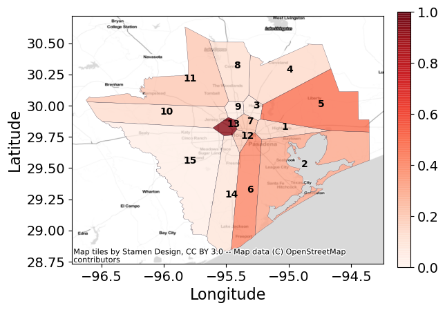
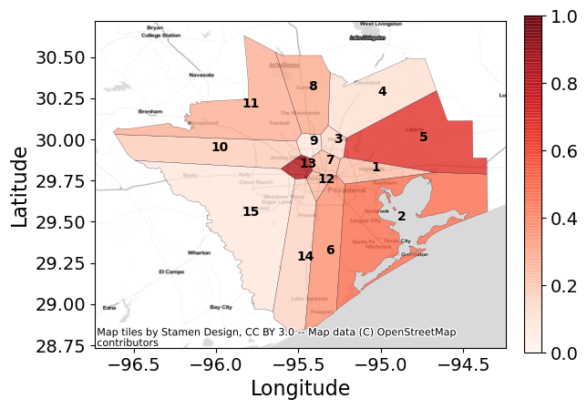
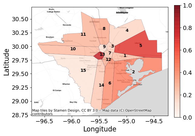
	(a-i)	(a-ii)	(a-iii)
Jan. ‘20
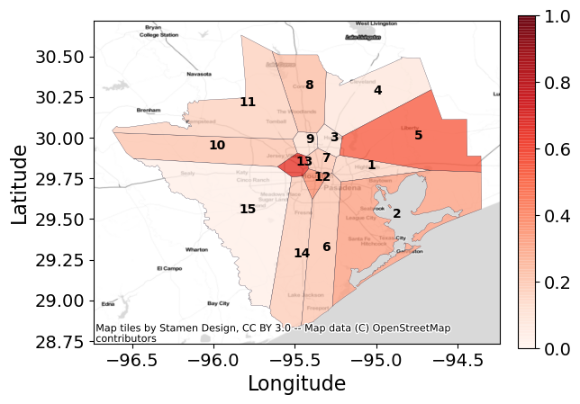
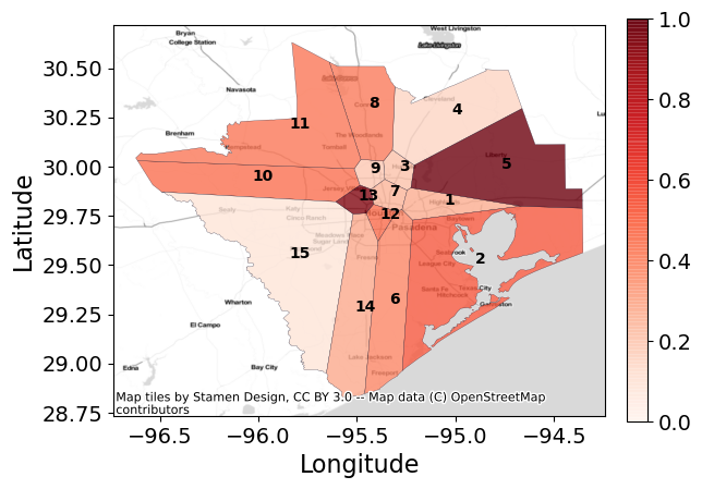
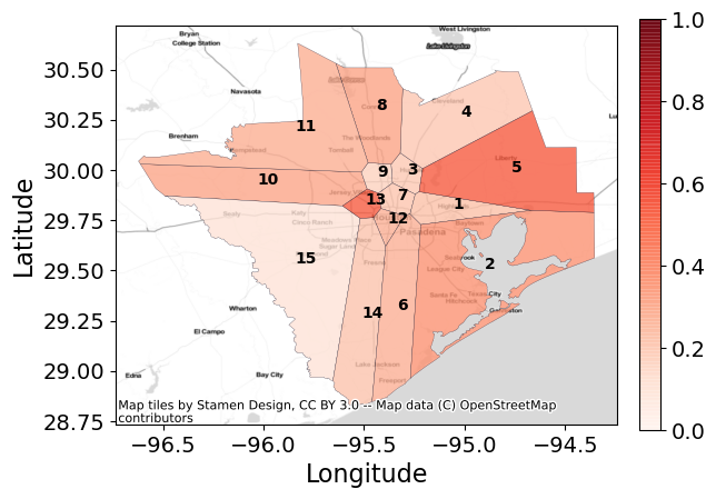
	(b-i)	(b-ii)	(b-iii)
Mar. ‘20
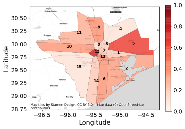
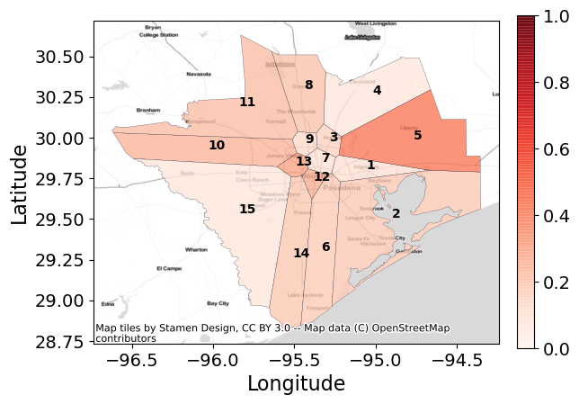
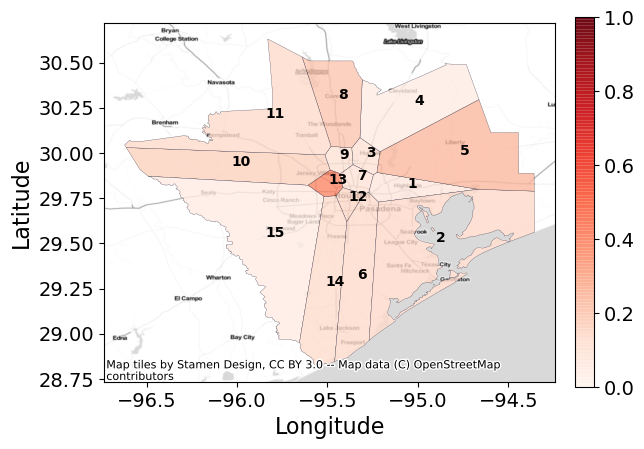
	(c-i)	(c-ii)	(c-iii)
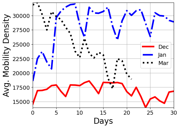
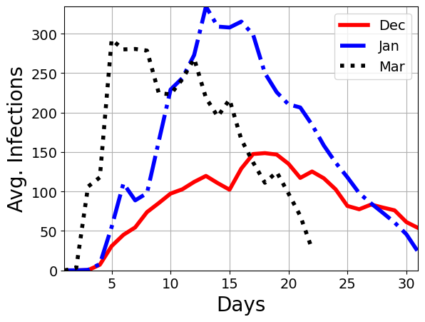
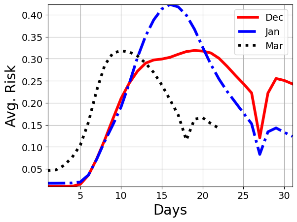
	(d-i)	(d-ii)	(d-iii)

Figure 8. Comparing the Risk across months in different regions of Houston (Harris County), TX. Panels (a), (b), and (c) show the evaluated risk ($\rho$) for each cluster (marked via numbers) for the months of Dec ‘19, Jan ‘20, and Mar ‘20, respectively. The panels (i), (ii), and (iii) show the risk varying over day 10, 15, and 20, respectively. In addition, panel (d-i), (d-ii), and (d-iii) show the comparison between the average number of location signals, infections and risk, across clusters over months, respectively. We observe that while the risk for months of Dec and Jan show similar trends for different days, the month of Mar has lower risk later in the month, which can be attributed to the drop in mobility; see cluster $5$ (best viewed digitally).

Appendix A Additional Experimental Results

	Day $10$	Day $15$	Day $20$
Dec. ‘19
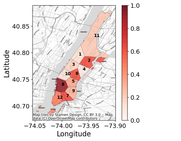
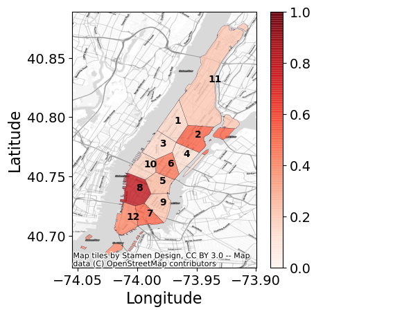
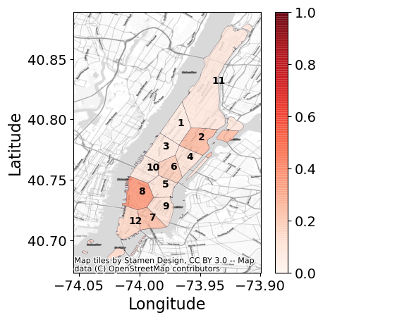
	(a-i)	(a-ii)	(a-iii)
Jan. ‘20
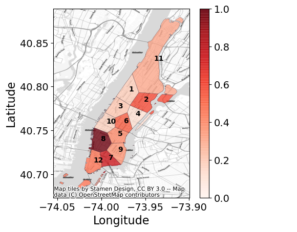
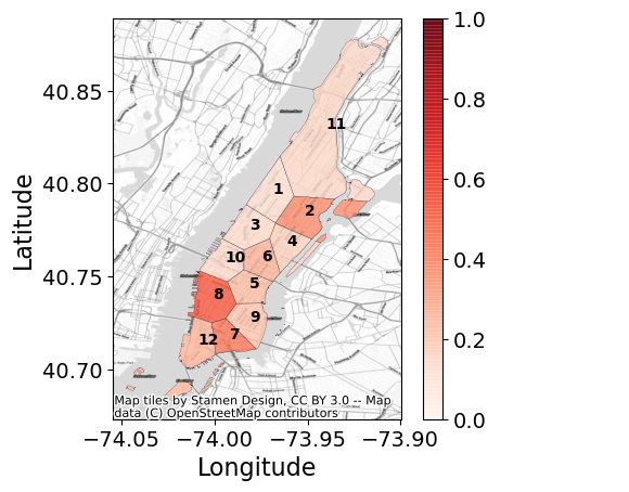
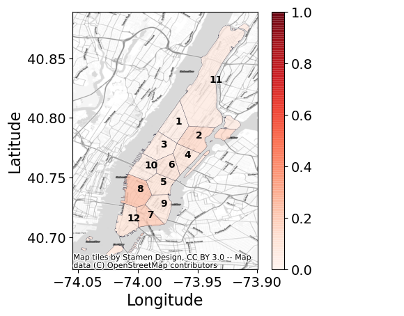
	(b-i)	(b-ii)	(b-iii)
Mar. ‘20
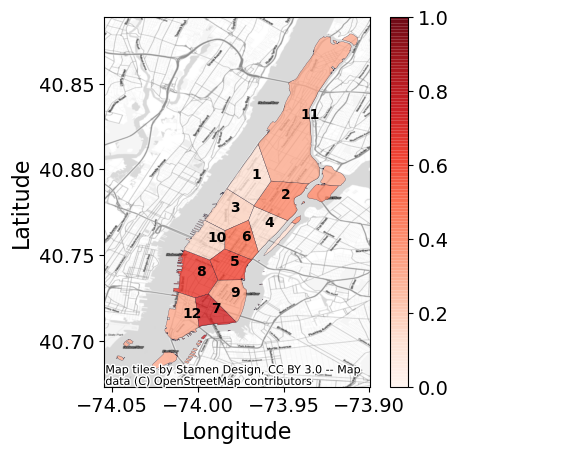
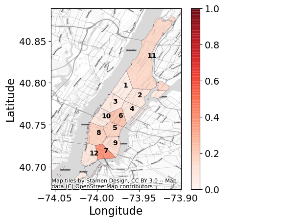
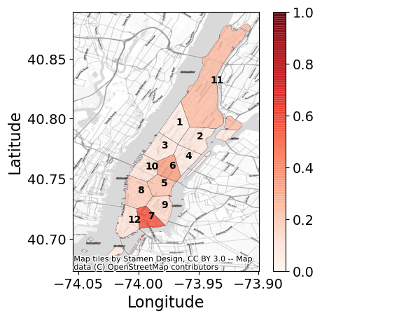
	(c-i)	(c-ii)	(c-iii)
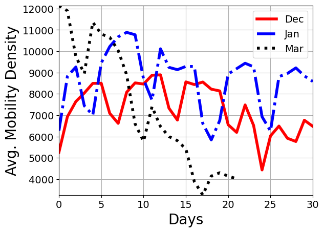
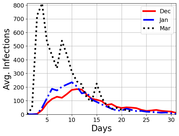
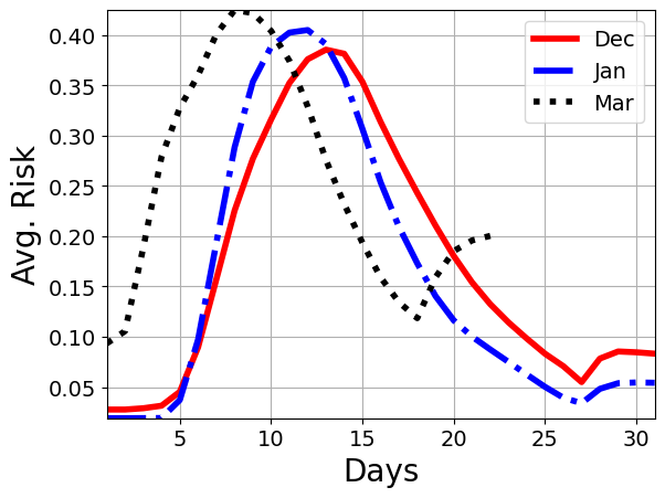
	(d-i)	(d-ii)	(d-iii)

Figure 11. Comparing the Risk across months in different regions of Manhattan (New York), NY. Panels (a), (b), and (c) show the evaluated risk ($\rho$) for each cluster (marked via numbers) for the months of Dec ‘19, Jan ‘20, and Mar ‘20, respectively. The panels (i), (ii), and (iii) show the risk varying over day 10, 15, and 20, respectively. In addition, panel (d-i), (d-ii), and (d-iii) show the comparison between the average number of location signals, infections and risk, across clusters over months, respectively. We observe that while the risk for months of Dec and Jan show similar trends for different days, the month of Mar has lower risk. This can be attributed to the drop in mobility.

	Day $10$	Day $15$	Day $20$
Dec. ‘19
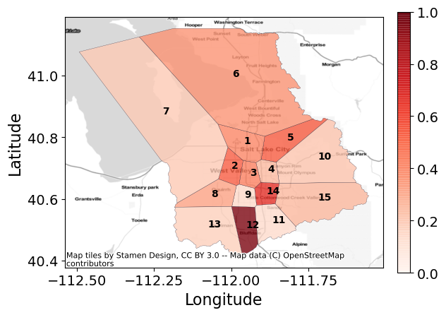
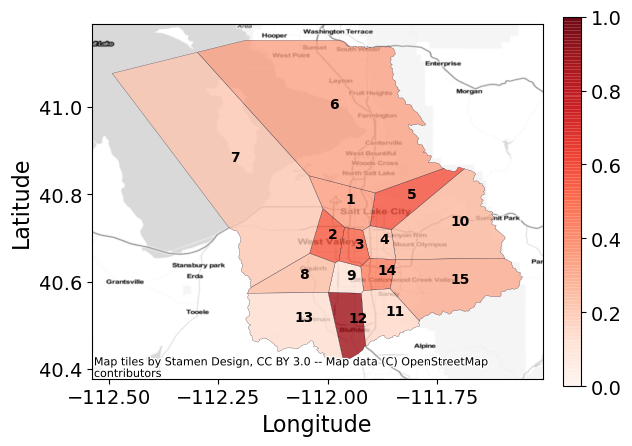
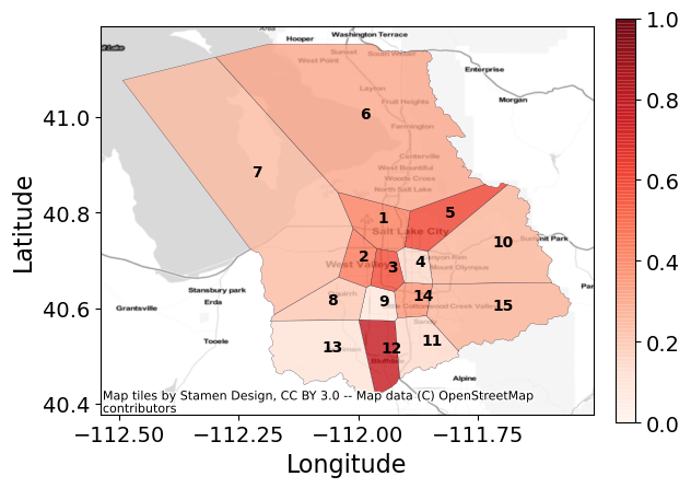
	(a-i)	(a-ii)	(a-iii)
Jan. ‘20
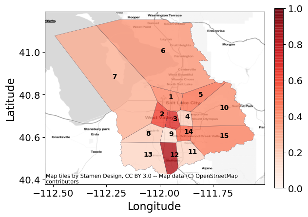
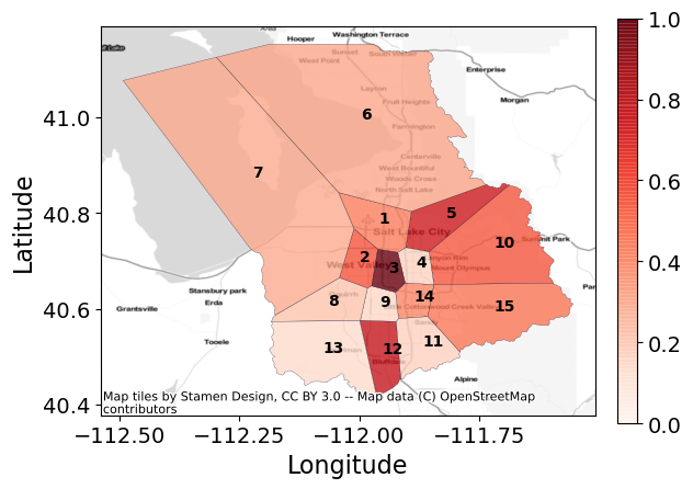
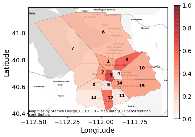
	(b-i)	(b-ii)	(b-iii)
Mar. ‘20
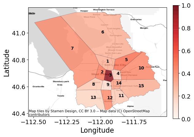
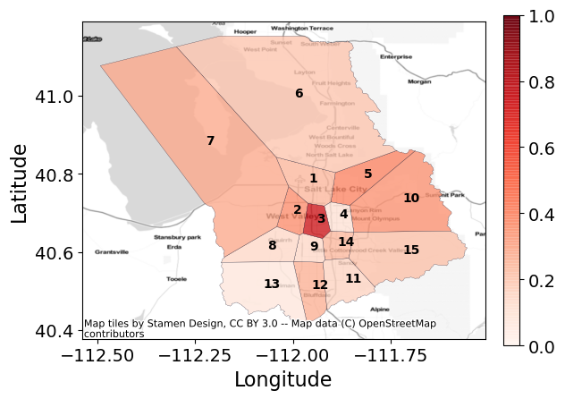
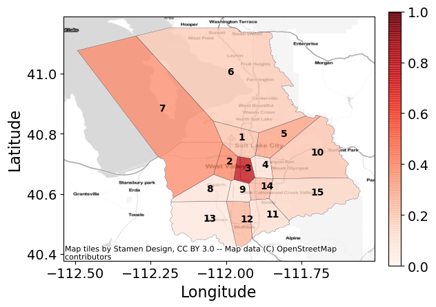
	(c-i)	(c-ii)	(c-iii)
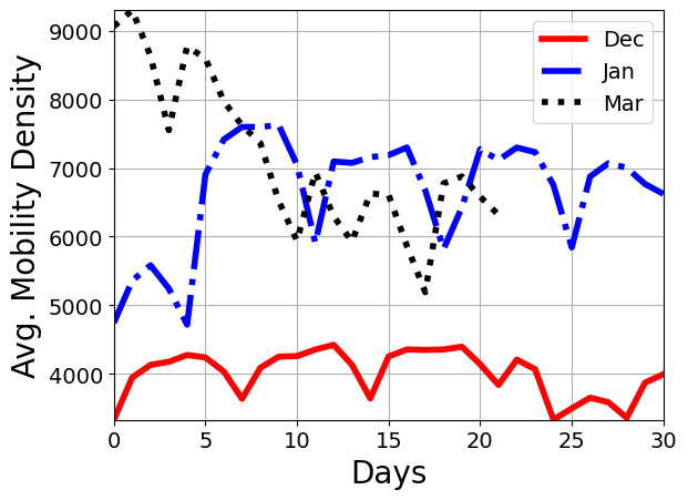
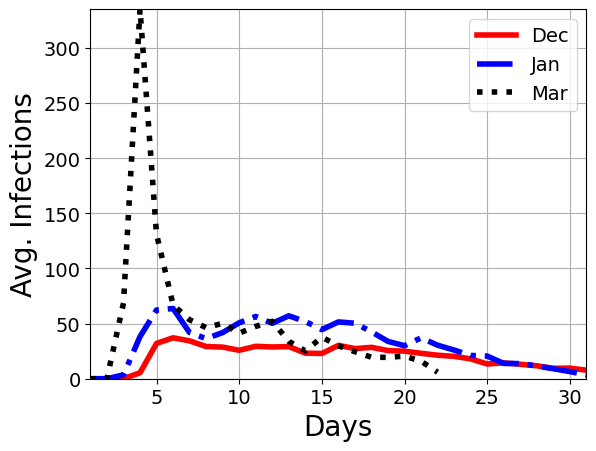
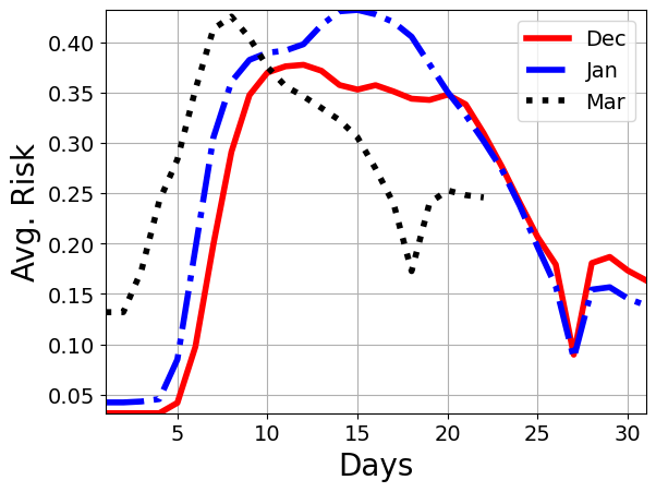
	(d-i)	(d-ii)	(d-iii)

Figure 12. Comparing the Risk across months in different regions of Salt Lake County, UT. Panels (a), (b), and (c) show the evaluated risk ($\rho$) for each cluster (marked via numbers) for the months of Dec ‘19, Jan ‘20, and Mar ‘20, respectively. The panels (i), (ii), and (iii) show the risk varying over day 10, 15, and 20, respectively.In addition, panel (d-i), (d-ii), and (d-iii) show the comparison between the average number of location signals, infections and risk, across clusters over months, respectively. We observe that while the risk for months of Dec and Jan show similar trends for different days, the month of Mar has lower risk. This can be attributed to the drop in mobility.

We ran our experiments, with the same setup described in Sec. 4, but for the areas around four more cities, namely Los Angeles, Seattle (King county), New York (Manhattan) and Salt Lake county. The statistics of these datasets can be found in Tables 9 and 9. The results are presented in Tables 10, 11, 12 and 13 and Figs. 9, 10, 11 and 12.

An interesting observation, in cities of New York (Manhattan) and Salt lake County shown in Fig 11 and Table 12, and Fig 12 and Table 13, respectively, is that an increased mobility in Mar. 2020 leading to a large number of infections decreases model’s capacity to predict later on when the infections drop. This is because the Hawkes process model tends to attribute the infections to the background rate $\mu_{c}$ rather than the mobility-dependent $R_{c}^{t}$. This leads to poor infection prediction performance (for all methods) since the model anticipates infections to happen at the relatively large background rate. In practice, such a modality can be avoided by using longer traces like (Chiang et al., 2020). Nevertheless, our risk scores (6) based on the intensity function $\lambda_{c}(t)$ (1) are still faithful to the infections since they take into account both the background rate and the mobility-dependence. This in fact highlights the advantages and reliability of the proposed risk score metric. In addition, our risk score for Manhattan (New York) also illustrates its applicability for fine-grained spatiotemporal risk assignment.

City	December	January	March
Los Angeles	$331\times 10^{6}$	282$\times 10^{6}$	171$\times 10^{6}$
Seattle	53$\times 10^{6}$	66$\times 10^{6}$	38$\times 10^{6}$
New York	41$\times 10^{6}$	36$\times 10^{6}$	21$\times 10^{6}$
Salt Lake	31$\times 10^{6}$	39$\times 10^{6}$	29$\times 10^{6}$

Table 8. Total No. location signals per Month

City	December	January	March
Los Angeles	159$\times 10^{3}$	171$\times 10^{3}$	131$\times 10^{3}$
Seattle	29$\times 10^{3}$	38$\times 10^{3}$	32$\times 10^{3}$
New York	40$\times 10^{3}$	41$\times 10^{3}$	32$\times 10^{3}$
Salt Lake	16$\times 10^{3}$	22$\times 10^{3}$	23$\times 10^{3}$

Table 9. No. Agents per Month

Model	Infection and Risk Prediction for Los Angeles, CA
	December ‘19				January ‘20				March ‘20
	$(\alpha,\beta,\Delta)=(2,2,5)$				$(\alpha,\beta,\Delta)=(2,2,5)$				$(\alpha,\beta,\Delta)=(2,2,5)$
	R-MAE(I)	$\sigma$(I)	MAE($\rho_{\mathrm{test}}$)	MAE($\rho_{\mathrm{all}}$)	R-MAE(I)	$\sigma$(I)	MAE($\rho_{\mathrm{test}})$	MAE($\rho_{\mathrm{all}}$)	R-MAE(I)	$\sigma$(I)	MAE($\rho_{\mathrm{test}}$)	MAE($\rho_{\mathrm{all}}$)
HawkesDen	0.249	0.099	0.105	0.047	0.526	0.091	0.148	0.101	0.517	0.054	0.162	0.133
LocationRisk@TMob	0.235	0.088	0.164	0.195	0.117	0.077	0.193	0.166	0.184	0.037	0.180	0.096
LocationRisk@T${}_{Mob^{+}}$	0.095	0.083	0.068	0.062	0.106	0.074	0.103	0.077	0.163	0.037	0.130	0.136

Table 10. Predicting (5-day) Infections and Risk for Los Angeles, CA. The table shows the error in predicted infections (I), the corresponding standard deviation, risk ($\rho$) for the test set, and over all days for Dec ‘19, Jan ‘20, and Mar ‘20 for the top-$5$ clusters.

	Day $10$	Day $15$	Day $20$
Dec. ‘19
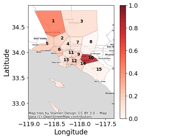
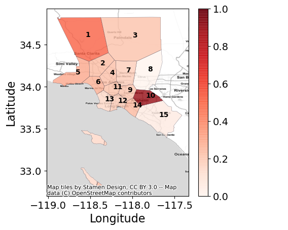
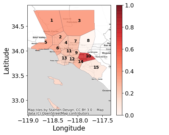
	(a-i)	(a-ii)	(a-iii)
Jan. ‘20
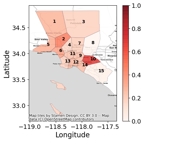
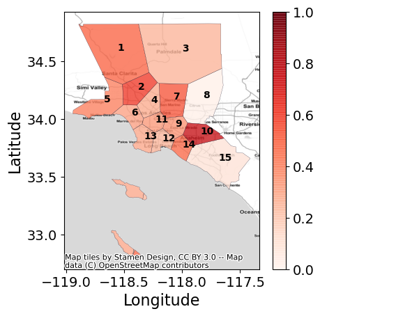
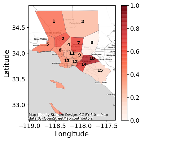
	(b-i)	(b-ii)	(b-iii)
Mar. ‘20
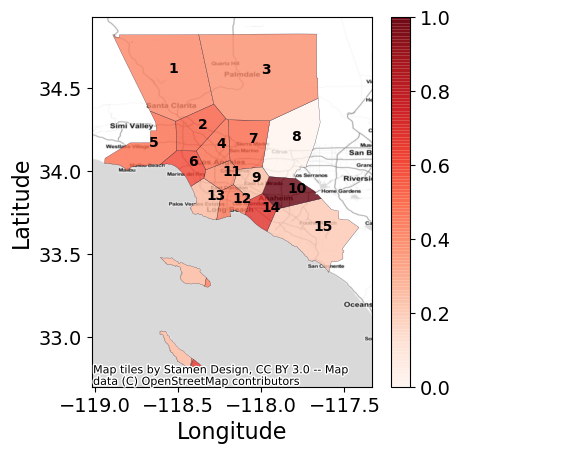
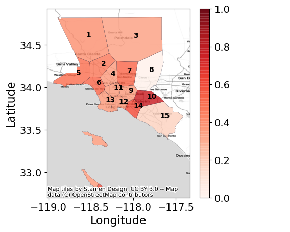
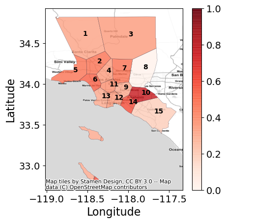
	(c-i)	(c-ii)	(c-iii)
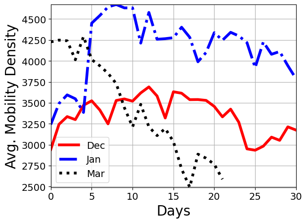
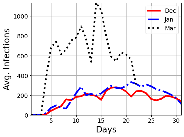
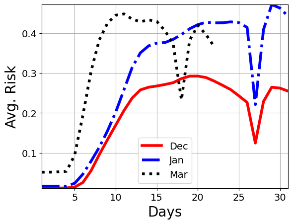
	(d-i)	(d-ii)	(d-iii)

Figure 9. Comparing the Risk across months in different regions of Los Angeles, CA. Panels (a), (b), and (c) show the evaluated risk ($\rho$) for each cluster (marked via numbers) for the months of Dec ‘19, Jan ‘20, and Mar ‘20, respectively. The panels (i), (ii), and (iii) show the risk varying over day 10, 15, and 20, respectively. In addition, panel (d-i), (d-ii), and (d-iii) show the comparison between the average number of location signals, infections and risk, across clusters over months, respectively. We observe that while the risk for months of Dec and Jan show similar trends for different days, the month of Mar has lower risk. This can be attributed to the drop in mobility.

Model	Infection and Risk Prediction for Seattle, WA
	December ‘19				January ‘20				March ‘20
	$(\alpha,\beta,\Delta)=(2,2,12)$				$(\alpha,\beta,\Delta)=(2,2,12)$				$(\alpha,\beta,\Delta)=(2,2,12)$
	R-MAE(I)	$\sigma$(I)	MAE($\rho_{\mathrm{test}}$)	MAE($\rho_{\mathrm{all}}$)	R-MAE(I)	$\sigma$(I)	MAE($\rho_{\mathrm{test}})$	MAE($\rho_{\mathrm{all}}$)	R-MAE(I)	$\sigma$(I)	MAE($\rho_{\mathrm{test}}$)	MAE($\rho_{\mathrm{all}}$)
HawkesDen	0.424	0.213	0.097	0.039	1.190	0.312	0.110	0.067	1.518	0.173	0.179	0.109
LocationRisk@TMob	0.259	0.198	0.075	0.038	0.756	0.267	0.100	0.052	1.329	0.168	0.206	0.115
LocationRisk@T${}_{Mob^{+}}$	0.227	0.195	0.077	0.032	0.614	0.254	0.085	0.055	0.504	0.131	0.155	0.104

Table 11. Predicting (5-day) Infections and Risk for Seattle, WA. The table shows the error in predicted infections (I), the corresponding standard deviation, risk ($\rho$) for the test set, and over all days for Dec ‘19, Jan ‘20, and Mar ‘20 for the top-$5$ clusters.

	Day $10$	Day $15$	Day $20$
Dec. ‘19
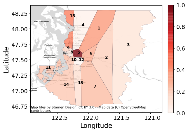
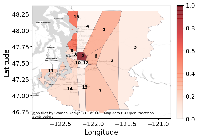
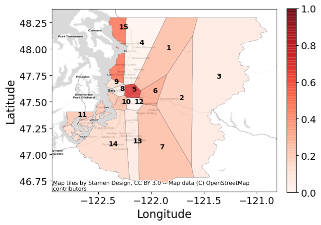
	(a-i)	(a-ii)	(a-iii)
Jan. ‘20
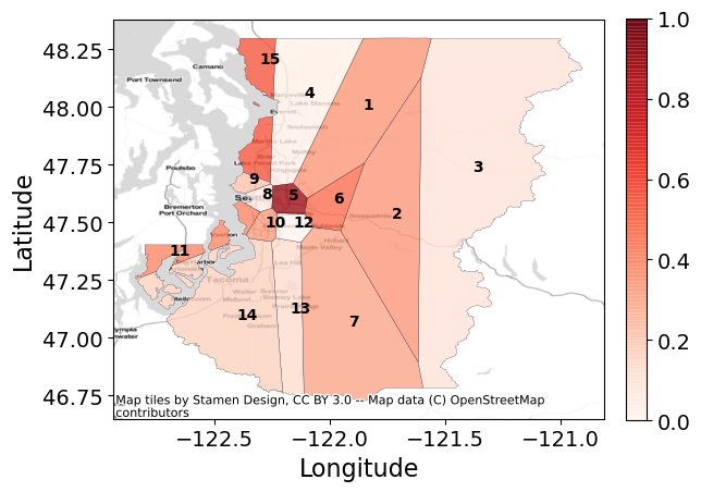
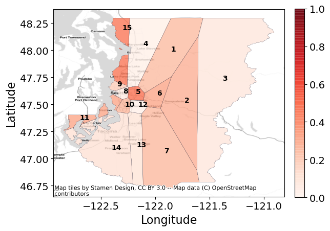
	(b-i)	(b-ii)	(b-iii)
Mar. ‘20
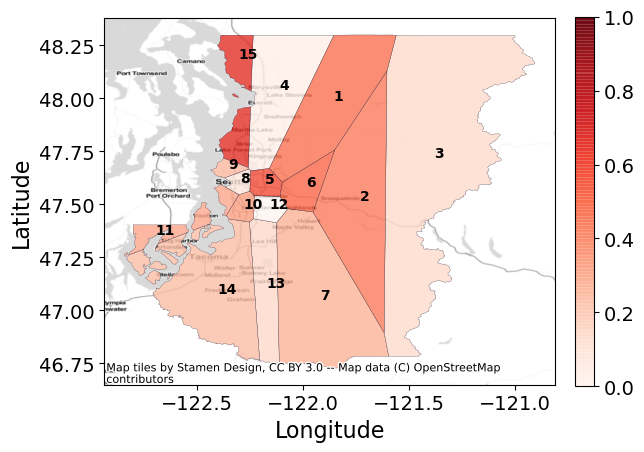
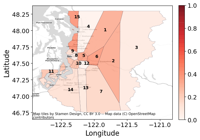
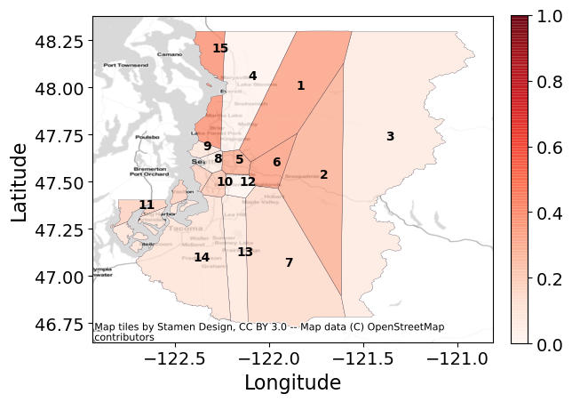
	(c-i)	(c-ii)	(c-iii)
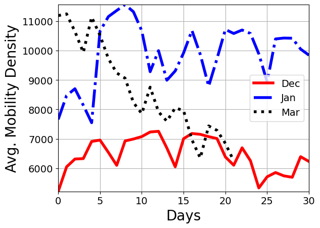
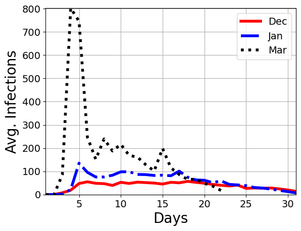
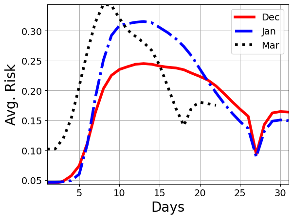
	(d-i)	(d-ii)	(d-iii)

Figure 10. Comparing the Risk across months in different regions of Seattle, WA. Panels (a), (b), and (c) show the evaluated risk ($\rho$) for each cluster (marked via numbers) for the months of Dec ‘19, Jan ‘20, and Mar ‘20, respectively. The panels (i), (ii), and (iii) show the risk varying over day 10, 15, and 20, respectively. In addition, panel (d-i), (d-ii), and (d-iii) show the comparison between the average number of location signals, infections and risk, across clusters over months, respectively. We observe that while the risk for months of Dec and Jan show similar trends for different days, the month of Mar has lower risk. This can be attributed to the drop in mobility.

Model	Infection and Risk Prediction for New York (Manhattan), NY
	December ‘19				January ‘20				March ‘20
	$(\alpha,\beta,\Delta)=(2,2,16)$				$(\alpha,\beta,\Delta)=(2,2,18)$				$(\alpha,\beta,\Delta)=(2,2,11)$
	R-MAE(I)	$\sigma$(I)	MAE($\rho_{\mathrm{test}}$)	MAE($\rho_{\mathrm{all}}$)	R-MAE(I)	$\sigma$(I)	MAE($\rho_{\mathrm{test}})$	MAE($\rho_{\mathrm{all}}$)	R-MAE(I)	$\sigma$(I)	MAE($\rho_{\mathrm{test}}$)	MAE($\rho_{\mathrm{all}}$)
HawkesDen	1.045	0.270	0.076	0.067	2.529∗	0.508∗	0.080∗	0.092∗	7.173	0.482	0.311	0.199
LocationRisk@TMob	0.210	0.170	0.035	0.058	1.068	0.356	0.060	0.089	7.446	0.492	0.344	0.205
LocationRisk@T${}_{Mob^{+}}$	0.145	0.162	0.021	0.061	0.448	0.294	0.037	0.080	4.440	0.370	0.248	0.174

Table 12. Predicting (5-day) Infections and Risk for New York (Manhattan), NY. The table shows the error in predicted infections (I), the corresponding standard deviation, risk ($\rho$) for the test set, and over all days for Dec ‘19, Jan ‘20, and Mar ‘20 for the top-$5$ clusters. ^∗ The model is essentially a constant model based on the $\chi^{2}$ statistic.

Model	Infection and Risk Prediction for Salt Lake County, UT
	December ‘19				January ‘20				March ‘20
	$(\alpha,\beta,\Delta)=(2,3,17)$				$(\alpha,\beta,\Delta)=(2,3,19)$				$(\alpha,\beta,\Delta)=(2,3,13)$
	R-MAE(I)	$\sigma$(I)	MAE($\rho_{\mathrm{test}}$)	MAE($\rho_{\mathrm{all}}$)	R-MAE(I)	$\sigma$(I)	MAE($\rho_{\mathrm{test}})$	MAE($\rho_{\mathrm{all}}$)	R-MAE(I)	$\sigma$(I)	MAE($\rho_{\mathrm{test}}$)	MAE($\rho_{\mathrm{all}}$)
HawkesDen	0.813∗	0.409∗	0.137∗	0.069∗	1.390	0.430	0.162	0.087	1.694	0.363	0.238	0.162
LocationRisk@TMob	0.197	0.298	0.070	0.062	0.624	0.335	0.110	0.072	1.133	0.308	0.198	0.141
LocationRisk@T${}_{Mob^{+}}$	0.189	0.287	0.069	0.059	0.429	0.308	0.088	0.066	1.064	0.307	0.234	0.167

Table 13. Predicting (5-day) Infections and Risk for Salt Lake County, UT. The table shows the error in predicted infections (I), the corresponding standard deviation, risk ($\rho$) for the test set, and over all days for Dec ‘19, Jan ‘20, and Mar ‘20 for the top-$5$ clusters. ^∗ The model is essentially a constant model based on the $\chi^{2}$ statistic.

References

- (1)
- sta (2020) 2020. Stay-at-home order. https://covid19.ca.gov/stay-home-except-for-essential-needs/#:~:text=All%20individuals%20living%20in%20the,the%20Questions%20%26%20Answers%20below). Accessed: 2020-11-10.
- ver (2020) 2020. Veraset Website. https://www.veraset.com/about-veraset. Accessed: 2020-10-25.
- Abrahamsson (1998) Torgil Abrahamsson. 1998. Estimation of origin-destination matrices using traffic counts-a literature survey. (1998).
- Bertozzi et al. (2020) Andrea L. Bertozzi, Elisa Franco, George Mohler, Martin B. Short, and Daniel Sledge. 2020. The challenges of modeling and forecasting the spread of COVID-19. Proceedings of the National Academy of Sciences 117, 29 (2020), 16732–16738. https://doi.org/10.1073/pnas.2006520117 arXiv:https://www.pnas.org/content/117/29/16732.full.pdf
- Bromage (2020) Erin Bromage. 2020. The Risks-Know Them-Avoid Them. Erin Bromage: COVID-19 Musings (2020).
- Chande et al. (2020) Aroon Chande, Seolha Lee, Mallory Harris, Quan Nguyen, Stephen J. Beckett, Troy Hilley, Clio Andris, and Joshua S. Weitz. 2020. Real-time, interactive website for US-county-level COVID-19 event risk assessment. Nature Human Behaviour (2020). https://doi.org/10.1038/s41562-020-01000-9
- Chang et al. (2020b) Serina Chang, Emma Pierson, Pang Wei Koh, Jaline Gerardin, Beth Redbird, David Grusky, and Jure Leskovec. 2020b. Mobility network models of COVID-19 explain inequities and inform reopening. Nature (2020), 1–6.
- Chang et al. (2020a) Sheryl L Chang, Nathan Harding, Cameron Zachreson, Oliver M Cliff, and Mikhail Prokopenko. 2020a. Modelling transmission and control of the COVID-19 pandemic in Australia. arXiv preprint arXiv:2003.10218 (2020).
- Chiang et al. (2020) Wen-Hao Chiang, Xueying Liu, and George Mohler. 2020. Hawkes process modeling of COVID-19 with mobility leading indicators and spatial covariates. medRxiv (2020). https://doi.org/10.1101/2020.06.06.20124149 arXiv:https://www.medrxiv.org/content/early/2020/06/08/2020.06.06.20124149.full.pdf
- Chu et al. (2020) Derek K Chu, Elie A Akl, Stephanie Duda, Karla Solo, Sally Yaacoub, Holger J Schünemann, Amena El-harakeh, Antonio Bognanni, Tamara Lotfi, Mark Loeb, et al. 2020. Physical distancing, face masks, and eye protection to prevent person-to-person transmission of SARS-CoV-2 and COVID-19: a systematic review and meta-analysis. The Lancet (2020).
- Delamater et al. (2019) Paul L Delamater, Erica J Street, Timothy F Leslie, Y Tony Yang, and Kathryn H Jacobsen. 2019. Complexity of the basic reproduction number (R0). Emerging infectious diseases 25, 1 (2019), 1.
- Eichler et al. (2017) Michael Eichler, Rainer Dahlhaus, and Johannes Dueck. 2017. Graphical modeling for multivariate hawkes processes with nonparametric link functions. Journal of Time Series Analysis 38, 2 (2017), 225–242.
- Evans et al. (2005) Neil D Evans, Lisa J White, Michael J Chapman, Keith R Godfrey, and Michael J Chappell. 2005. The structural identifiability of the susceptible infected recovered model with seasonal forcing. Mathematical biosciences 194, 2 (2005), 175–197.
- Farrington et al. (2003) CP Farrington, MN Kanaan, and NJ Gay. 2003. Branching process models for surveillance of infectious diseases controlled by mass vaccination. Biostatistics 4, 2 (2003), 279–295.
- Ferguson et al. (2020) Neil Ferguson, Daniel Laydon, Gemma Nedjati Gilani, Natsuko Imai, Kylie Ainslie, Marc Baguelin, Sangeeta Bhatia, Adhiratha Boonyasiri, ZULMA Cucunuba Perez, Gina Cuomo-Dannenburg, et al. 2020. Report 9: Impact of non-pharmaceutical interventions (NPIs) to reduce COVID19 mortality and healthcare demand. (2020).
- Ferguson et al. (2006) Neil M Ferguson, Derek AT Cummings, Christophe Fraser, James C Cajka, Philip C Cooley, and Donald S Burke. 2006. Strategies for mitigating an influenza pandemic. Nature 442, 7101 (2006), 448–452.
- Ferretti et al. (2020) Luca Ferretti, Chris Wymant, Michelle Kendall, Lele Zhao, Anel Nurtay, Lucie Abeler-Dörner, Michael Parker, David Bonsall, and Christophe Fraser. 2020. Quantifying SARS-CoV-2 transmission suggests epidemic control with digital contact tracing. Science 368, 6491 (2020).
- for Disease Control (CDC) (2020) Center for Disease Control (CDC). 2020. Coronavirus Disease 2019 (COVID-19): Daily Activities and Going Out. https://www.cdc.gov/coronavirus/2019-ncov/daily-life-coping/going-out.html. Accessed: 2020-11-12.
- Granger (1969) Clive WJ Granger. 1969. Investigating causal relations by econometric models and cross-spectral methods. Econometrica: journal of the Econometric Society (1969), 424–438.
- Halloran et al. (2008) M Elizabeth Halloran, Neil M Ferguson, Stephen Eubank, Ira M Longini, Derek AT Cummings, Bryan Lewis, Shufu Xu, Christophe Fraser, Anil Vullikanti, Timothy C Germann, et al. 2008. Modeling targeted layered containment of an influenza pandemic in the United States. Proceedings of the National Academy of Sciences 105, 12 (2008), 4639–4644.
- He et al. (2020) Xi He, Eric HY Lau, Peng Wu, Xilong Deng, Jian Wang, Xinxin Hao, Yiu Chung Lau, Jessica Y Wong, Yujuan Guan, Xinghua Tan, et al. 2020. Temporal dynamics in viral shedding and transmissibility of COVID-19. Nature medicine 26, 5 (2020), 672–675.
- Hengartner and Fenimore (2018) Nicolas Hengartner and Paul Fenimore. 2018. Quantifying Model Form Uncertainty of Epidemic Forecasting Models from Incidence Data. Online Journal of Public Health Informatics 10, 1 (2018).
- Institute (2020) Harvard Global Health Institute. 2020. Key Metrics for COVID Suppression. https://globalepidemics.org/key-metrics-for-covid-suppression/. Accessed: 2020-11-12.
- Kamra et al. (2020) Nitin Kamra, Yizhou Zhang, Sirisha Rambhatla, Chuizheng Meng, and Yan Liu. 2020. PolSIRD: Modeling Epidemic Spread under Intervention Policies and an Application to the Spread of COVID-19. arXiv:q-bio.PE/2009.01894
- Keeling et al. (2020) Matt J Keeling, T Deirdre Hollingsworth, and Jonathan M Read. 2020. Efficacy of contact tracing for the containment of the 2019 novel coronavirus (COVID-19). Journal of Epidemiology & Community Health 74, 10 (2020), 861–866. https://doi.org/10.1136/jech-2020-214051 arXiv:https://jech.bmj.com/content/74/10/861.full.pdf
- Kermack and McKendrick (1927) William Ogilvy Kermack and Anderson G McKendrick. 1927. A contribution to the mathematical theory of epidemics. Proceedings of the royal society of london. Series A, Containing papers of a mathematical and physical character 115, 772 (1927), 700–721.
- Kerr et al. (2020) Cliff C Kerr, Robyn M Stuart, Dina Mistry, Romesh G Abeysuriya, Gregory Hart, Katherine Rosenfeld, Prashanth Selvaraj, Rafael C Nunez, Brittany Hagedorn, Lauren George, et al. 2020. Covasim: an agent-based model of COVID-19 dynamics and interventions. medRxiv (2020).
- Kiamari et al. (2020) Mehrdad Kiamari, Gowri Ramachandran, Quynh Nguyen, Eva Pereira, Jeanne Holm, and Bhaskar Krishnamachari. 2020. COVID-19 Risk Estimation using a Time-varying SIR-model. 1st ACM SIGSPATIAL International Workshop on Modeling and Understanding the Spread of COVID-19 (2020).
- Kresin et al. (2020) Conor Kresin, Frederic Paik Schoenberg, and George Mohler. 2020. Comparison of the Hawkes and SEIR models for the spread of Covid-19. (2020).
- Li et al. (2011) Jing Li, Daniel Blakeley, et al. 2011. The failure of R 0. Computational and mathematical methods in medicine 2011 (2011).
- Li et al. (2020) Qun Li, Xuhua Guan, Peng Wu, Xiaoye Wang, Lei Zhou, Yeqing Tong, Ruiqi Ren, Kathy SM Leung, Eric HY Lau, Jessica Y Wong, et al. 2020. Early transmission dynamics in Wuhan, China, of novel coronavirus–infected pneumonia. New England Journal of Medicine (2020).
- Li et al. (2018) Yaguang Li, Rose Yu, Cyrus Shahabi, and Yan Liu. 2018. Diffusion Convolutional Recurrent Neural Network: Data-Driven Traffic Forecasting. In International Conference on Learning Representations. https://openreview.net/forum?id=SJiHXGWAZ
- Lotfi et al. (2020) Melika Lotfi, Michael R Hamblin, and Nima Rezaei. 2020. COVID-19: Transmission, prevention, and potential therapeutic opportunities. Clinica Chimica Acta (2020).
- Meyer et al. (2015) Sebastian Meyer, Leonhard Held, and Michael Höhle. 2015. Spatiotemporal analysis of epidemic phenomena using the R package surveillance. Statistics-Computation 1411.0416 (2015).
- Miller et al. (2020) Andrew C Miller, Nicholas J Foti, Joseph A Lewnard, Nicholas P Jewell, Carlos Guestrin, and Emily B Fox. 2020. Mobility trends provide a leading indicator of changes in SARS-CoV-2 transmission. medRxiv (2020). https://doi.org/10.1101/2020.05.07.20094441 arXiv:https://www.medrxiv.org/content/early/2020/05/11/2020.05.07.20094441.full.pdf
- Mohler et al. (2020) George Mohler, Frederic Schoenberg, Martin B Short, and Daniel Sledge. 2020. Analyzing the World-Wide Impact of Public Health Interventions on the Transmission Dynamics of COVID-19. arXiv preprint arXiv:2004.01714 (2020).
- Osthus et al. (2017) Dave Osthus, Kyle S Hickmann, Petruţa C Caragea, Dave Higdon, and Sara Y Del Valle. 2017. Forecasting seasonal influenza with a state-space SIR model. The annals of applied statistics 11, 1 (2017), 202.
- Pei and Shaman (2020) Sen Pei and Jeffrey Shaman. 2020. Initial Simulation of SARS-CoV2 Spread and Intervention Effects in the Continental US. medRxiv (2020).
- Rizoiu et al. (2018) Marian-Andrei Rizoiu, Swapnil Mishra, Quyu Kong, Mark Carman, and Lexing Xie. 2018. SIR-Hawkes: linking epidemic models and Hawkes processes to model diffusions in finite populations. In Proceedings of the 2018 World Wide Web Conference. 419–428.
- Roosa and Chowell (2019) Kimberlyn Roosa and Gerardo Chowell. 2019. Assessing parameter identifiability in compartmental dynamic models using a computational approach: application to infectious disease transmission models. Theoretical Biology and Medical Modelling 16, 1 (2019), 1.
- Times (2020a) New York Times. 2020a. Actual Coronavirus Infections Vastly Under counted, C.D.C. Data Shows. https://www.nytimes.com/2020/06/27/health/coronavirus-antibodies-asymptomatic.html. Accessed: 2020-10-27.
- Times (2020b) New York Times. 2020b. As the Coronavirus Surges, a New Culprit Emerges: Pandemic Fatigue. https://www.nytimes.com/2020/10/17/us/coronavirus-pandemic-fatigue.html. Accessed: 2020-10-29.
- Times (2020c) New York Times. 2020c. As Virus Surges in Europe, Resistance to New Restrictions Also Grows. https://www.nytimes.com/2020/10/09/world/europe/coronavirus-europe-fatigue.html. Accessed: 2020-10-29.
- Wiersinga et al. (2020) W Joost Wiersinga, Andrew Rhodes, Allen C Cheng, Sharon J Peacock, and Hallie C Prescott. 2020. Pathophysiology, transmission, diagnosis, and treatment of coronavirus disease 2019 (COVID-19): a review. Jama 324, 8 (2020), 782–793.
- Yuan et al. (2019) Baichuan Yuan, Hao Li, Andrea L Bertozzi, P Jeffrey Brantingham, and Mason A Porter. 2019. Multivariate spatiotemporal hawkes processes and network reconstruction. SIAM Journal on Mathematics of Data Science 1, 2 (2019), 356–382.
- Zou et al. (2020) Difan Zou, Lingxiao Wang, Pan Xu, Jinghui Chen, Weitong Zhang, and Quanquan Gu. 2020. Epidemic Model Guided Machine Learning for COVID-19 Forecasts in the United States. medRxiv (2020).