Strichartz estimates in Wiener amalgam spaces and applications to nonlinear wave equations

Abstract.

In this paper we obtain some new Strichartz estimates for the wave propagator $e^{it\sqrt{-\Delta}}$ in the context of Wiener amalgam spaces. While it is well understood for the Schrödinger case, nothing is known about the wave propagator. This is because there is no such thing as an explicit formula for the integral kernel of the propagator unlike the Schrödinger case. To overcome this lack, we instead approach the kernel by rephrasing it as an oscillatory integral involving Bessel functions and then by carefully making use of cancellation in such integrals based on the asymptotic expansion of Bessel functions. Our approach can be applied to the Schrödinger case as well. We also obtain some corresponding retarded estimates to give applications to nonlinear wave equations where Wiener amalgam spaces as solution spaces can lead to a finer analysis of the local and global behavior of the solution.

1. Introduction

The space-time integrability of the wave propagator $e^{it\sqrt{-\Delta}}$, known as Strichartz estimates, has been extensively studied over the past several decades and is completely understood:

$$\|e^{it\sqrt{-\Delta}}f\|_{L_{t}^{q}L_{x}^{r}}\lesssim\|f\|_{\dot{H}^{\sigma}},$$ (1.1)

where $(q,r)$ is wave-admissible, i.e., $2\leq q\leq\infty$, $2\leq r<\infty$,

$$\frac{2}{q}+\frac{n-1}{r}\leq\frac{n-1}{2}\quad\text{and}\quad\frac{1}{q}+\frac{n}{r}=\frac{n}{2}-\sigma.$$ (1.2)

The diagonal case $q=r$ was obtained in [18] in connection with the restriction theorems for the cone. See [15, 12] for the general case $q\neq r$.

In this paper we are concerned with obtaining these Strichartz estimates in Wiener amalgam spaces which, unlike the $L^{p}$ spaces, control the local regularity of a function and its decay at infinity separately. This separability makes it possible to perform a finer analysis of the local and global behavior of the propagator. These aspects were originally pointed out in the several works by Cordero and Nicola [3, 4, 5] in the context of the Schrödinger propagator $e^{it\Delta}$, although the spaces were first introduced by Feichtinger [6] and have already appeared as a technical tool in the study of partial differential equations ([19]). See also [16].

While it is well understood for the Schrödinger case, nothing is known about the wave propagator. The arguments used for the former case take advantage of the explicit formula for the integral kernel of $e^{it\Delta}$. This makes it possible to obtain some time-deay estimates just by calculating the kernel directly on Wiener amalgam spaces, and ultimately to appeal to the Keel-Tao approach [12]. However, it is no longer available for the wave case in which there is no such thing as an explicit formula for the corresponding kernel.

To overcome this lack, we instead consider the problem of obtaining a pointwise estimate for the integral kernel of the Fourier multiplier ${|\nabla|}^{-\sigma}e^{it\sqrt{-\Delta}}$ by rephrasing it as an oscillatory integral involving Bessel functions using polar coordinates and then by carefully estimating such integrals on Wiener amalgam spaces based on the asymptotic expansion of Bessel functions. Our approach in this paper is different from that of Cordero and Nicola mentioned above, and can be applied to the Schrödinger case as well ([13]).

Before stating our results, we recall the definition of Wiener amalgam spaces. Let $\varphi\in C_{0}^{\infty}$ be a test function satisfying $\|\varphi\|_{L^{2}}=1$. Let $1\leq p,q\leq\infty$. Then the Wiener amalgam space $W(p,q)$ is defined as the space of functions $f\in L_{\textrm{loc}}^{p}$ equipped with the norm

$$\|f\|_{W(p,q)}=\big{\|}\,\|f\tau_{x}\varphi\|_{L^{p}}\big{\|}_{L_{x}^{q}},$$

where $\tau_{x}\varphi(\cdot)=\varphi(\cdot-x)$. Here different choices of $\varphi$ generate the same space and yield equivalent norms. This space can be seen as a natural extension of $L^{p}$ space in view of $W(p,p)=L^{p}$, and $W(A,B)$ for Banach spaces $A$ and $B$ is also defined in the same way. We also list some basic properties of these spaces which will be frequently used in the sequel:

• Inclusion; if  $p_{0}\geq p_{1}$ and $q_{0}\leq q_{1}$,

  $$W(p_{0},q_{0})\subset W(p_{1},q_{1}).$$ (1.3)

• Convolution; if $1/p+1=1/p_{0}+1/p_{1}$ and $1/q+1=1/q_{0}+1/q_{1}$,

  $$W(p_{0},q_{0})*W(p_{1},q_{1})\subset W(p,q).$$ (1.4)

• Interpolation; if  $q_{0}<\infty$ or $q_{1}<\infty$,

  $$(W(p_{0},q_{0}),W(p_{1},q_{1}))_{[\theta]}=W(p_{\theta},q_{\theta}).$$ (1.5)

• Duality; if $p,q<\infty$,

  $$W(p,q)^{\prime}=W(p^{\prime},q^{\prime}).$$ (1.6)

We refer to [6, 7, 8, 10] for details.

1.1. Strichartz estimates in Wiener amalgam spaces

Our main results for the Strichartz estimates are now stated as follows.

Theorem 1.1.

Let $n\geq 3$ and $\frac{n}{4}<\sigma<\frac{n-1}{2}$. Assume that $2\leq\widetilde{q}<q<\infty$ and

$$\frac{2n}{n-2\sigma}<r\leq\widetilde{r}<\begin{cases}\frac{4}{n-4\sigma+1}\quad\text{if}\quad\sigma<\frac{n}{4}+\frac{1}{2(n-1)},\\ \frac{2n}{n-2\sigma-1}\quad\text{if}\quad\sigma\geq\frac{n}{4}+\frac{1}{2(n-1)}.\end{cases}$$ (1.7)

Then we have

$$\|e^{it\sqrt{-\Delta}}f\|_{W({\widetilde{q}},q)_{t}W({\widetilde{r}},r)_{x}}\lesssim\|f\|_{\dot{H}^{\sigma}}$$ (1.8)

if

$$\frac{1}{\widetilde{q}}+\frac{n-1}{\widetilde{r}}>\frac{n}{2}-\sigma\quad\text{and}\quad\frac{1}{q}+\frac{n}{r}=\frac{n}{2}-\sigma.$$ (1.9)

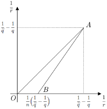
Figure 1. The region of $(1/r,1/\widetilde{r})$ for (1.8)

Remark 1.2.

Roughly speaking, the estimate (1.8) shows that the $W(\widetilde{r},r)_{x}$-norm of the propagator has a $L_{t}^{q}$-decay at infinity. But the second condition in (1.9) becomes equivalent to the scaling condition for the classical estimates (1.1). Hence, our estimates are better than the classical ones for large time since the classical $L_{x}^{r}$ norm in (1.1) is rougher than the $W(\widetilde{r},r)_{x}$-norm when $r<\widetilde{r}$ (see (1.3)), although locally the classical $L_{t}^{q}$ regularity is replaced by $L_{t}^{\widetilde{q}}$ with $\widetilde{q}<q$. In this regard, it is worth trying to obtain (1.8) especially when $r<\widetilde{r}$, and the theorem shows that $(1/r,1/\widetilde{r})$ can lie in some region inside the triangle with vertices $O,A,B$ in Figure 1. Note here that (1.9) determines the line through $A$ and $B$, $1/\widetilde{q}-1/q=n/r-(n-1)/\widetilde{r}$. Some estimates when $r>\widetilde{r}$ are of course derived trivially from the classical ones (1.1) using the inclusion relation (1.3).

Remark 1.3.

From complex interpolation (see (1.5)) between (1.8) and the classical estimates (1.1), we can easily obtain further estimates on Wiener amalgam spaces extending the range of $\sigma$ to $0\leq\sigma<n/2$. In a different way, one can also trivially increase $q,r$ and diminish $\widetilde{q},\widetilde{r}$ in (1.8) using the inclusion relation (1.3).

We also obtain the corresponding retarded estimates which are useful to control nonlinearities in relevant nonlinear problems discussed below.

Theorem 1.4.

Let $n\geq 3$ and $\gamma\in(\frac{n}{2},\frac{n+1}{2})\cup(\frac{n+1}{2},{n-1})$. Assume that

$$0<\frac{1}{q}+\frac{1}{q_{1}}<\frac{1}{\widetilde{q}}+\frac{1}{\widetilde{q}_{1}}\leq 1\quad(q\neq\infty)$$

and

$$\max\big{\{}\frac{n-2\gamma+1}{2},\,\frac{n-\gamma-1}{n}\big{\}}<\frac{1}{\widetilde{r}}+\frac{1}{\widetilde{r}_{1}}\leq\frac{1}{r}+\frac{1}{r_{1}}<\frac{n-\gamma}{n}.$$

Then we have

$$\bigg{\|}\int_{0}^{t}e^{i(t-s)\sqrt{-\Delta}}|\nabla|^{-\gamma}F(\cdot,s)ds\bigg{\|}_{W(\widetilde{q},q)_{t}W(\widetilde{r},r)_{x}}\lesssim\|F\|_{W({\widetilde{q}}_{1}^{\prime},q_{1}^{\prime})_{t}W(\widetilde{r}_{1}^{\prime},r_{1}^{\prime})_{x}}$$ (1.10)

if

$$\frac{1}{\widetilde{q}}+\frac{1}{\widetilde{q}_{1}}+\frac{n-1}{\widetilde{r}}+\frac{n-1}{\widetilde{r}_{1}}>n-\gamma\quad\text{and}\quad\frac{1}{q}+\frac{1}{q_{1}}+\frac{n}{r}+\frac{n}{r_{1}}=n-\gamma.$$ (1.11)

Remark 1.5.

It is well known that some retarded estimates can be derived from the homogeneous estimates using the $TT^{\ast}$ argument and the Christ-Kiselev lemma [2]. But this standard method is not accessible in the context of Wiener amalgam spaces because of lack of the corresponding lemma, and therefore we need to approach the matter more directly.

1.2. Application to nonlinear wave equations

Now we turn to a few applications of our estimates to local well-posedness of the Cauchy problem for nonlinear wave equations

$$\begin{cases}\partial_{t}^{2}u-\Delta u=F_{k}(u),\\ u(x,0)=f(x)\in\dot{H}^{\sigma},\\ \partial_{t}u(x,0)=g(x)\in\dot{H}^{\sigma-1},\end{cases}$$ (1.12)

where $(x,t)\in\mathbb{R}^{n}\times\mathbb{R}$ and the nonlinearity $F_{k}\in C^{1}(\mathbb{R})$ ($k>1$) satisfies

$$|F_{k}(u)|\lesssim|u|^{k}\quad\text{and}\quad|u||F_{k}^{\prime}(u)|\sim|F_{k}(u)|.$$ (1.13)

The typical models are when $F_{k}(u)=\pm u^{k}$ or $\pm|u|^{k-1}u$.

The problem of determining the largest $k$ for which (1.12) is locally well-posed was addressed for higher dimensions $n\geq 3$ in [11], and then almost completely answered ([14, 15, 12]); the problem (1.12) is ill-posed when

$$k>k(\sigma)=\begin{cases}1+\frac{4}{n+1-4\sigma}\quad\text{if}\quad\sigma\leq 1/2,\\ 1+\frac{4}{n-2\sigma}\quad\text{if}\quad\sigma\geq 1/2.\end{cases}$$ (1.14)

The endpoint case $\sigma=0$ ($k=2$) when $n=3$ is also ill-posed. When $\sigma\geq\frac{n-3}{2(n-1)}$, it is known that $k(\sigma)$ given by (1.14) is indeed best-possible, but for $\sigma<\frac{n-3}{2(n-1)}(<1/2)$ the sharpness is not yet known. The piecewise smooth curve in Figure 2 describes the maximal $k$ particularly when $n=3$.

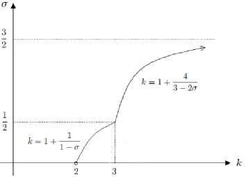
Figure 2. The maximal $k(\sigma)$ for $n=3$

The second aim in this paper is to study this nonlinear problem in the context of Wiener amalgam spaces by making use of our estimates. The motivation behind this is that these spaces as solution spaces can control the local regularity of the solution and its decay at infinity separately. This can lead to a finer analysis of the local and global behavior of the solution. Since the case $\sigma\geq 1/2$ was settled for all dimensions $n\geq 3$, we shall only discuss in detail the low-regularity case $\sigma\leq 1/2$ although the former case can be also handled in the same way. We shall also restrict ourselves to three physical dimension $n=3$ just for brevity since the proof of our existence results for higher dimensions $n\geq 4$ follows similar lines.

Theorem 1.6.

Let $0<\sigma\leq 1/2$ and $1<k<k(\sigma)$. Then there exist a time $T>0$ and a unique solution $u$ to (1.12) with

$$u\in W(\widetilde{q},q)_{t}([0,T];W(\widetilde{r},r)_{x}(\mathbb{R}^{3}))$$ (1.15)

where

$$\begin{gathered}0<\frac{1}{q}<\frac{1}{\widetilde{q}}\leq\frac{1}{4},\quad\frac{1}{4}<\frac{1}{\widetilde{r}}\leq\frac{1}{r}<\frac{1}{2},\\ 1\leq\frac{1}{q}+\frac{3}{r}<\min\big{\{}\frac{3}{2}-\frac{2}{\widetilde{q}},\,\frac{2}{\widetilde{q}}+\frac{4}{\widetilde{r}}-\frac{1}{2}\big{\}}.\end{gathered}$$ (1.16)

Furthermore, the solution satisfies

$$u\in C_{t}([0,T];\dot{H}^{\sigma})\cap C_{t}^{1}([0,T];\dot{H}^{\sigma-1})$$ (1.17)

and depends continuously (in the norms (1.15),(1.17)) on the data.

From the proof one can give a precise estimate for the life span of the solution according to the size of the initial data as

$$T\sim(\|f\|_{\dot{H}^{\sigma}}+\|g\|_{\dot{H}^{\sigma-1}})^{-c(k-1)}$$

for some $c=c(q,\widetilde{q},r,\widetilde{r},k)>0$ (see (6.11)). Once the local existence is shown for small $T$, it holds therefore for any finite time $T$ by a straightforward iteration using

$$\sup_{t\in[0,T]}\|u\|_{\dot{H}^{\sigma}}+\sup_{t\in[0,T]}\|u\|_{\dot{H}^{\sigma-1}}\lesssim\|f\|_{\dot{H}^{\sigma}}+\|g\|_{\dot{H}^{\sigma-1}}$$

(see (6.16),(6.17)).

Outline of the paper. In Section 2 we prove Theorem 1.1; using the $TT^{\ast}$ argument we first rephrase (1.8) as

$$\bigg{\|}\int_{\mathbb{R}}(K_{2\sigma}(\cdot,t-s)*F(\cdot,s))(x)ds\bigg{\|}_{W(\widetilde{q},q)_{t}W(\widetilde{r},r)_{x}}\lesssim\|F\|_{W(\widetilde{q}^{\prime},q^{\prime})_{t}W(\widetilde{r}^{\prime},r^{\prime})_{x}}$$

where $K_{\gamma}$ denotes the integral kernel of the Fourier multiplier $|\nabla|^{-\gamma}e^{it\sqrt{-\Delta}}$ given as in (2.2), and then make use of the convolution relation to reduce the matter to $\|K_{2\sigma}\|_{W(L^{\frac{\widetilde{q}}{2}},L^{\frac{q}{2},\infty})_{t}W(\frac{\widetilde{r}}{2},\frac{r}{2})_{x}}<\infty.$ This is carried out by estimating the time-decay estimates $\|K_{2\sigma}(\cdot,t)\|_{W(\frac{\widetilde{r}}{2},\frac{r}{2})_{x}}\lesssim|t|^{-\omega}$ with suitable $\omega(r,\widetilde{r},\sigma,n)>0$ to insure $|t|^{-\omega}\in W(L^{\frac{\widetilde{q}}{2}},L^{\frac{q}{2},\infty})_{t}$ under the second condition in (1.9). To obtain such decay estimates (Proposition 2.1), we first rephrase the kernel in Section 3 as an oscillatory integral like (3) involving Bessel functions to carefully estimate it making use of cancellation in such integrals based on the asymptotic expansion of Bessel functions, and then use these estimations (Proposition 3.1) to calculate the time-decay bounds in Section 4. Section 5 is devoted to proving the corresponding retarded estimates in Theorem 1.4, and finally we apply the Strichartz estimates to the nonlinear problem (1.12) to prove Theorem 1.6 in the final section, Section 6.

Throughout this paper, the letter $C$ stands for a positive constant which may be different at each occurrence. We also denote $A\lesssim B$ to mean $A\leq CB$ with unspecified constants $C>0$.

2. Homogeneous estimates

In this section we prove Theorem 1.1. To prove (1.8), we can apply the standard TT* argument because of the Hölder’s type inequality

$$|\langle F,G\rangle_{L^{2}_{x,t}}|\leq\|F\|_{W(\widetilde{q},q)_{t}W(\widetilde{r},r)_{x}}\|G\|_{W({\widetilde{q}}^{\prime},q^{\prime})_{t}W({\widetilde{r}}^{\prime},r^{\prime})_{x}}$$

which can be proved directly from the definition of Wiener amalgam spaces. Hence it is enough to show that

$$\bigg{\|}\int_{\mathbb{R}}|\nabla|^{-2\sigma}e^{i(t-s)\sqrt{-\Delta}}F(\cdot,s)ds\bigg{\|}_{W(\widetilde{q},q)_{t}W(\widetilde{r},r)_{x}}\lesssim\|F\|_{W(\widetilde{q}^{\prime},q^{\prime})_{t}W(\widetilde{r}^{\prime},r^{\prime})_{x}}.$$ (2.1)

We first write the integral kernel of the Fourier multiplier $|\nabla|^{-\gamma}e^{it\sqrt{-\Delta}}$ as

$$K_{\gamma}(x,t):=\frac{1}{(2\pi)^{n}}\int_{\mathbb{R}^{n}}e^{i(x\cdot\xi+t|\xi|)}\frac{d\xi}{|\xi|^{\gamma}}.$$ (2.2)

Then (2.1) is rephrased as follows:

$$\bigg{\|}\int_{\mathbb{R}}(K_{2\sigma}(\cdot,t-s)*F(\cdot,s))(x)ds\bigg{\|}_{W(\widetilde{q},q)_{t}W(\widetilde{r},r)_{x}}\lesssim\|F\|_{W(\widetilde{q}^{\prime},q^{\prime})_{t}W(\widetilde{r}^{\prime},r^{\prime})_{x}}.$$ (2.3)

Now we will prove (2.3). By Minkowski’s inequality and the convolution relation (1.4), it follows that

$$\bigg{\|}\int_{\mathbb{R}}(K_{2\sigma}(\cdot,t-s)* F(\cdot,s))(x)ds\bigg{\|}_{W(\widetilde{q},q)_{t}W(\widetilde{r},r)_{x}}$$

$$\leq\bigg{\|}\int_{\mathbb{R}}\|K_{2\sigma}(\cdot,t-s)*F(\cdot,s)\|_{W(\widetilde{r},r)_{x}}ds\bigg{\|}_{W(\widetilde{q},q)_{t}}$$

$$\leq\bigg{\|}\int_{\mathbb{R}}\|K_{2\sigma}(\cdot,t-s)\|_{W(\frac{\widetilde{r}}{2},\frac{r}{2})_{x}}\|F(\cdot,s)\|_{W(\widetilde{r}^{\prime},r^{\prime})_{x}}ds\bigg{\|}_{W(\widetilde{q},q)_{t}}.$$ (2.4)

Recall the Hardy-Littlewood-Sobolev fractional integration theorem (see e.g. [17], p. 119) in dimension $1$:

$$L^{\frac{1}{\alpha},\infty}\ast L^{p}\hookrightarrow L^{q}$$ (2.5)

for $0<\alpha<1$ and $1\leq p<q<\infty$ with $\frac{1}{q}+1=\frac{1}{p}+\alpha$. Using (2.5) with $\alpha=\frac{2}{q}$ and $p=q^{\prime}$ and the usual Young’s inequality, the convolution relation again gives

$$W(L^{\frac{\widetilde{q}}{2}},L^{\frac{q}{2},\infty})_{t}*W(\widetilde{q}^{\prime},q^{\prime})_{t}\subset W(\widetilde{q},q)_{t}$$

for $2\leq\widetilde{q}\leq\infty$ and $2<q<\infty$. Hence we get

$$\bigg{\|}\int_{\mathbb{R}}\|K_{2\sigma}(\cdot,t-s)\|_{W(\frac{\widetilde{r}}{2},\frac{r}{2})_{x}} \|F(\cdot,s)\|_{W(\widetilde{r}^{\prime},r^{\prime})_{x}}ds\bigg{\|}_{W(\widetilde{q},q)_{t}}$$

$$\lesssim \|K_{2\sigma}\|_{{W(L^{\frac{\widetilde{q}}{2}},L^{\frac{q}{2},\infty})_{t}}{W(\frac{\widetilde{r}}{2},\frac{r}{2})_{x}}}\|F\|_{W(\widetilde{q}^{\prime},q^{\prime})_{t}W(\widetilde{r}^{\prime},r^{\prime})_{x}}.$$ (2.6)

Combining (2) and (2), we now obtain the desired estimate (2.3) if

$$\|K_{2\sigma}\|_{{W(L^{\frac{\widetilde{q}}{2}},L^{\frac{q}{2},\infty})_{t}}{W(\frac{\widetilde{r}}{2},\frac{r}{2})_{x}}}<\infty$$ (2.7)

for $(\widetilde{q},\widetilde{r})$ and $(q,r)$ satisfying the same conditions as in Theorem 1.1.

To show (2.7), we use the following time-decay estimates for the integral kernel (2.2) which will be obtained in later sections.

Proposition 2.1.

Let $n\geq 3$ and $\gamma\in(\frac{n}{2},\frac{n+1}{2})\cup(\frac{n+1}{2},n-1)$. Assume that

$$\frac{2n}{n-\gamma}<r\leq\widetilde{r}<\begin{cases}\frac{4}{n-2\gamma+1}\quad\text{if}\quad\gamma<\frac{n}{2}+\frac{1}{n-1},\\ \frac{2n}{n-\gamma-1}\quad\text{if}\quad\gamma\geq\frac{n}{2}+\frac{1}{n-1}.\end{cases}$$ (2.8)

Then we have

$$\|K_{\gamma}(\cdot,t)\|_{W(\frac{\widetilde{r}}{2},\frac{r}{2})_{x}}\lesssim\begin{cases}|t|^{-n+\gamma+{2(n-1)}/{\widetilde{r}}}\quad\text{if}\quad|t|\leq 1,\\ |t|^{-n+\gamma+{2n}/{r}}\quad\text{if}\quad|t|\geq 1.\end{cases}$$ (2.9)

To begin with, we set $h(t)=\|K_{2\sigma}(\cdot,t)\|_{W(\frac{\widetilde{r}}{2},\frac{r}{2})_{x}}$ and choose $\varphi(t)\in C_{0}^{\infty}(\mathbb{R})$ supported on $\{t\in\mathbb{R}:|t|\leq 1\}$. To calculate $\|h\|_{{W(L^{\frac{\widetilde{q}}{2}},L^{\frac{q}{2},\infty})_{t}}}$ using (2.9), we handle $\|h\tau_{k}\varphi\|_{L_{t}^{\widetilde{q}/2}}$ dividing cases into $|k|\leq 1$, $1\leq|k|\leq 2$ and $|k|\geq 2$. First we consider the case $|k|\leq 1$. By using (2.9) with $\gamma=2\sigma$ and the support condition of $\varphi$,

$$\|h\tau_{k}\varphi\|_{L_{t}^{\tilde{q}/2}}^{\widetilde{q}/2}\lesssim\int_{0<|t|\leq 1}|t|^{\frac{\widetilde{q}}{2}(-n+2\sigma+\frac{2(n-1)}{\widetilde{r}})}dt+\int_{1\leq|t|\leq|k|+1}|t|^{\frac{\widetilde{q}}{2}(-n+2\sigma+\frac{2n}{r})}dt.$$ (2.10)

Since $\frac{\widetilde{q}}{2}(-n+2\sigma+\frac{2(n-1)}{\widetilde{r}})+1>0$ by the first condition in (1.9), the first integral in (2.10) is trivially finite. The second integral is bounded as follows:

$$\int_{1\leq|t|\leq|k|+1}|t|^{\frac{\widetilde{q}}{2}(-n+2\sigma+\frac{2n}{r})}dt \lesssim\frac{(|k|+1)^{\frac{\widetilde{q}}{2}(-n+2\sigma+\frac{2n}{r})+1}-1}{\frac{\widetilde{q}}{2}(-n+2\sigma+\frac{2n}{r})+1}$$

$$\lesssim|k|.$$ (2.11)

Indeed, since ${\frac{\widetilde{q}}{2}(-n+2\sigma+\frac{2n}{r})}<0$ by the first inequality in the condition (1.7), the second inequality in (2) follows easily from the mean value theorem. Hence we get

$$\|h\tau_{k}\varphi\|_{L_{t}^{\widetilde{q}/2}}^{\widetilde{q}/2}\lesssim 1$$

when $|k|\leq 1$. The other cases $1\leq|k|\leq 2$ and $|k|\geq 2$ are handled in the same way:

$$\|h\tau_{k}\varphi\|_{L_{t}^{\widetilde{q}/2}}^{\widetilde{q}/2} \lesssim\int_{|k|-1\leq|t|\leq 1}|t|^{\frac{\widetilde{q}}{2}(-n+2\sigma+\frac{2(n-1)}{\widetilde{r}})}dt+\int_{1\leq|t|\leq|k|+1}|t|^{\frac{\widetilde{q}}{2}(-n+2\sigma+\frac{2n}{r})}dt$$

$$\lesssim 1+|k|$$

$$\lesssim 1$$

when $1\leq|k|\leq 2$, and when $|k|\geq 2$

$$\|h\tau_{k}\varphi\|_{L_{t}^{\widetilde{q}/2}}^{\widetilde{q}/2} \lesssim\int_{{|k|-1}\leq|t|\leq{|k|+1}}|t|^{\frac{\widetilde{q}}{2}(-n+2\sigma+\frac{2n}{r})}dt$$

$$\lesssim\frac{(|k|+1)^{\frac{\widetilde{q}}{2}(-n+2\sigma+\frac{2n}{r})+1}-(|k|-1)^{\frac{\widetilde{q}}{2}(-n+2\sigma+\frac{2n}{r})+1}}{\frac{\widetilde{q}}{2}(-n+2\sigma+\frac{2n}{r})+1}$$

$$\lesssim(|k|-1)^{\frac{\widetilde{q}}{2}(-n+2\sigma+\frac{2n}{r})}.$$

Consequently, we get

$$\|h\tau_{k}\varphi\|_{L_{t}^{\widetilde{q}/2}}\lesssim\begin{cases}1\quad\textit{if}\quad|k|\leq 2,\\ (|k|-1)^{-(n-2\sigma-\frac{2n}{r})}\quad\textit{if}\quad|k|\geq 2.\end{cases}$$ (2.12)

By (2.12), $\|h\tau_{k}\varphi\|_{L_{t}^{\widetilde{q}/2}}$ belongs to $L^{\frac{q}{2},\infty}_{k}$ since we are assuming the second condition in (1.9) which is equivalent to $\frac{2}{q}=n-2\sigma-\frac{2n}{r}$. This finally implies

$$\|h\|_{{W(L^{\frac{\widetilde{q}}{2}},L^{\frac{q}{2},\infty})_{t}}}<\infty$$

for $(\widetilde{q},\widetilde{r})$ and $(q,r)$ satisfying the same conditions as in Theorem 1.1 except for the case $\sigma=(n+1)/4$ when $n\geq 4$. But this case can be shown by just interpolating the cases $\sigma=(n+1)/4-\varepsilon$ and $\sigma=(n+1)/4+\varepsilon$ with a sufficiently small $\varepsilon>0$. Note finally that the condition $q>\widetilde{q}$ in the theorem follows immediately from combining (1.9) and $r\leq\widetilde{r}$.

3. Pointwise estimates for the integral kernel

In this section we first obtain the following pointwise estimates for the integral kernel (2.2) which will be used in the next section to finish the proof of the time-decay estimates (Proposition 2.1):

Proposition 3.1.

Let $n\geq 3$. If $n\geq 4$ and $(n+1)/2<\gamma<n-1$,

$$|K_{\gamma}(x,t)|\lesssim\begin{cases}|x|^{-(n-\gamma)}\quad\text{if}\quad|x|\geq|t|/2,\\ |t|^{-1}|x|^{-(n-1-\gamma)}\quad\text{if}\quad\quad|x|\leq|t|/2,\end{cases}$$ (3.1)

and if $(n-1)/2<\gamma<(n+1)/2$

$$|K_{\gamma}(x,t)|\lesssim\begin{cases}|x|^{-\frac{n-1}{2}}\big{|}|x|-|t|\big{|}^{-(\frac{n+1}{2}-\gamma)}\quad{\text{if}}\quad|x|\geq|t|/2,\\ |t|^{-1}|x|^{-(n-1-\gamma)}\quad{\text{if}}\quad|x|\leq|t|/2.\end{cases}$$ (3.2)

(If $1/2<\gamma<1$, (3.2) is still true for $n=2$).

Proof.

Using polar coordinates $\xi=\omega\xi^{\prime}$ and $x=rx^{\prime}$ where $\xi^{\prime},x^{\prime}\in\mathbb{S}^{n-1}$, $\omega=|\xi|$ and $r=|x|$, we first write

$$K_{\gamma}(x,t) =\frac{1}{(2\pi)^{n}}\int_{0}^{\infty}e^{it\omega}\omega^{n-\gamma-1}\int_{\mathbb{S}^{n-1}}e^{ir\omega x^{\prime}\cdot\xi^{\prime}}d\xi^{\prime}d\omega$$

$$=C_{n}r^{-\frac{n-2}{2}}\int_{0}^{\infty}e^{it\omega}\omega^{\frac{n}{2}-\gamma}J_{\frac{n-2}{2}}(r\omega)d\omega.$$ (3.3)

Here we also used the fact (see, for example, [9], p. 428) that

$$\int_{\mathbb{S}^{n-1}}e^{ir\omega x^{\prime}\cdot\xi^{\prime}}d\xi^{\prime}=C_{n}(r\omega)^{-\frac{n-2}{2}}J_{\frac{n-2}{2}}(r\omega)$$

where $J_{\nu}$ denotes the Bessel function of complex order $\nu$ with $\text{Re}\,\nu>-1/2$.

3.1. The case $\frac{n+1}{2}<\gamma<n-1$

In this case we will obtain

$$|K_{\gamma}(x,t)|\lesssim\min\big{\{}|x|^{-n+\gamma},|t|^{-1}|x|^{-n+\gamma+1}\big{\}}$$

which implies (3.1). We first show $|K_{\gamma}(x,t)|\lesssim|x|^{-n+\gamma}$. Motivated by the following fact (see, for example, [9], Appendix B) that for $\text{Re}\,\nu>-1/2$

$$|J_{\nu}(m)|\leq\begin{cases}C_{\nu}m^{\text{Re}\nu}\quad\text{if}\quad 0<m<1,\\ C_{\nu}m^{-\frac{1}{2}}\quad\text{if}\quad m\geq 1,\end{cases}$$ (3.4)

we first split the integral in (3) into the regions $r\omega<1$ and $r\omega>1$:

$$\int_{0}^{1/r}e^{it\omega}\omega^{\frac{n}{2}-\gamma}J_{\frac{n-2}{2}}(r\omega)d\omega+\int_{1/r}^{\infty}e^{it\omega}\omega^{\frac{n}{2}-\gamma}J_{\frac{n-2}{2}}(r\omega)d\omega.$$ (3.5)

Using (3.4), the first part is then bounded as

$$\bigg{|}\int_{0}^{1/r}e^{it\omega}\omega^{\frac{n}{2}-\gamma}J_{\frac{n-2}{2}}(r\omega)d\omega\bigg{|} \lesssim\int_{0}^{1/r}\omega^{\frac{n}{2}-\gamma}\big{|}J_{\frac{n-2}{2}}(r\omega)\big{|}d\omega$$

$$\lesssim\int_{0}^{1/r}\omega^{\frac{n}{2}-\gamma}(r\omega)^{\frac{n-2}{2}}d\omega$$

$$\lesssim r^{\frac{n-2}{2}}r^{-n+\gamma}$$ (3.6)

when $\gamma<n$. A similar argument gives the same bound for the second part under the condition $\gamma>(n+1)/2$, and thus

$$|K_{\gamma}(x,t)|\lesssim|x|^{-n+\gamma},$$

if $\frac{n+1}{2}<\gamma<n$ (which is wider than what we want in the first place).

To show $|K_{\gamma}(x,t)|\lesssim|t|^{-1}|x|^{-n+\gamma+1}$ this time, we start with applying integration by parts to the integral in (3) as

$$\int_{0}^{\infty}e^{it\omega}\omega^{\frac{n}{2}-\gamma}J_{\frac{n-2}{2}}(r\omega)d\omega=-\int_{0}^{\infty}\frac{e^{it\omega}}{it}\frac{d}{d\omega}\big{(}\omega^{\frac{n}{2}-\gamma}J_{\frac{n-2}{2}}(r\omega)\big{)}d\omega,$$ (3.7)

where the boundary terms vanish when $\frac{n-1}{2}<\gamma<n-1$; using (3.4),

$$\bigg{|}\frac{e^{it\omega}}{it}r^{-\frac{n-2}{2}}\omega^{\frac{n}{2}-\gamma}J_{\frac{n-2}{2}}(r\omega)\bigg{|}\lesssim\begin{cases}|t|^{-1}\omega^{n-1-\gamma}\rightarrow 0\quad\text{as}\quad\omega\rightarrow 0,\\ |t|^{-1}r^{-\frac{n-1}{2}}\omega^{\frac{n-1}{2}-\gamma}\rightarrow 0\quad\text{as}\quad\omega\rightarrow\infty.\end{cases}$$

We then use the following property (see, for example, [9], p. 425)

$$\frac{d}{dm}(m^{-\nu}J_{\nu}(m))=-m^{-\nu}J_{\nu+1}(m)\quad\text{for}\quad\text{Re}\,\nu>-1/2,$$

to estimate the derivative term in (3.7) as

$$\frac{d}{d\omega}\bigg{(}\omega^{\frac{n}{2}-\gamma}r^{-\frac{n-2}{2}}J_{\frac{n-2}{2}}(r\omega)\bigg{)} =\frac{d}{d\omega}\bigg{(}(r\omega)^{-\frac{n-2}{2}}J_{\frac{n-2}{2}}(r\omega)\cdot\omega^{n-\gamma-1}\bigg{)}$$

$$=Cr^{-\frac{n-2}{2}}\omega^{\frac{n-2}{2}-\gamma}J_{\frac{n-2}{2}}(r\omega)-r^{-\frac{n-4}{2}}\omega^{\frac{n}{2}-\gamma}J_{\frac{n}{2}}(r\omega).$$

Hence we arrive at

$$r^{-\frac{n-2}{2}}\int_{0}^{\infty}e^{it\omega}\omega^{\frac{n}{2}-\gamma}J_{\frac{n-2}{2}}(r\omega)d\omega= -Cr^{-\frac{n-2}{2}}\int_{0}^{\infty}\frac{e^{it\omega}}{it}\omega^{\frac{n-2}{2}-\gamma}J_{\frac{n-2}{2}}(r\omega)d\omega$$ (3.8)

$$+r^{-\frac{n-4}{2}}\int_{0}^{\infty}\frac{e^{it\omega}}{it}\omega^{\frac{n}{2}-\gamma}J_{\frac{n}{2}}(r\omega)d\omega.$$

By splitting the integrals in the right side of (3.8) into the regions $r\omega<1$ and $r\omega>1$, and using (3.4) as above, one can see that

$$\bigg{|}\int_{0}^{\infty}\frac{e^{it\omega}}{it}\omega^{\frac{n-2}{2}-\gamma}J_{\frac{n-2}{2}}(r\omega)d\omega\bigg{|}\lesssim|t|^{-1}r^{-n/2+\gamma}$$ (3.9)

if $\frac{n-1}{2}<\gamma<n-1$, and if $\frac{n+1}{2}<\gamma<n+1$

$$\bigg{|}\int_{0}^{\infty}\frac{e^{it\omega}}{it}\omega^{\frac{n}{2}-\gamma}J_{\frac{n}{2}}(r\omega)d\omega\bigg{|}\lesssim|t|^{-1}r^{-n/2+\gamma-1}.$$

Combining these estimates, we therefore get for $\frac{n+1}{2}<\gamma<n-1$

$$\bigg{|}\int_{0}^{\infty}e^{it\omega}\omega^{\frac{n}{2}-\gamma}J_{\frac{n-2}{2}}(r\omega)d\omega\bigg{|}\lesssim|t|^{-1}r^{\frac{n-2}{2}}r^{-n+\gamma+1}$$

which implies immediately

$$|K_{\gamma}(x,t)|\lesssim|t|^{-1}|x|^{-n+\gamma+1}$$

from (3).

3.2. The case $\frac{n-1}{2}<\gamma<\frac{n+1}{2}$ ($1/2<\gamma<1$ if $n=2$)

In order to obtain this case, we shall make use of the following asymptotic expansion of Bessel functions (see, for example, [9], Appendix B) for the region $r\omega>1$ in the previous argument, and use cancellation in $e^{i(t\pm r)\omega}$.

Lemma 3.2.

For $m>1$ and $\text{Re}\,\nu>-1/2$,

$$J_{\nu}(m)=\frac{1}{\sqrt{2\pi m}}\big{(}e^{i(m-\frac{\pi\nu}{2}-\frac{\pi}{4})}+e^{-i(m-\frac{\pi\nu}{2}-\frac{\pi}{4})}\big{)}+R_{\nu}(m)$$ (3.10)

where

$$|R_{\nu}(m)|\leq C_{\nu}m^{-3/2}.$$ (3.11)

Inserting (3.10) into the second integral in (3.5), we now see that

$$\int_{1/r}^{\infty}e^{it\omega}\omega^{\frac{n}{2}-\gamma}J_{\frac{n-2}{2}}(r\omega)d\omega =\frac{1}{\sqrt{2\pi}}e^{-i\frac{\pi(n-1)}{4}}r^{-1/2}\int_{1/r}^{\infty}e^{i(t+r)\omega}\omega^{\frac{n-1}{2}-\gamma}d\omega$$

$$+\frac{1}{\sqrt{2\pi}}e^{i\frac{\pi(n-1)}{4}}r^{-1/2}\int_{1/r}^{\infty}e^{i(t-r)\omega}\omega^{\frac{n-1}{2}-\gamma}d\omega$$

$$+\int_{1/r}^{\infty}e^{it\omega}\omega^{\frac{n}{2}-\gamma}R_{\frac{n-2}{2}}(r\omega)d\omega.$$ (3.12)

To bound the first integral in the right side of (3.2), we first denote $A=t+r$ and may assume $A>0$ without loss of generality. We also set $\alpha=\gamma-\frac{n-1}{2}$. Changing variables $A\omega\rightarrow\omega$ and using the fact that $e^{i\omega}$ is periodic with period $2\pi$, we now see that

$$\int_{1/r}^{\infty}e^{i(t+r)\omega}\omega^{\frac{n-1}{2}-\gamma}d\omega =A^{\alpha-1}\sum_{k=0}^{\infty}\int_{\frac{A}{r}+2\pi k}^{\frac{A}{r}+2\pi(k+1)}\omega^{-\alpha}e^{i\omega}d\omega$$

$$=A^{\alpha-1}\sum_{k=0}^{\infty}\bigg{[}\int_{\frac{A}{r}+2\pi k}^{\frac{A}{r}+2\pi k+\pi}\omega^{-\alpha}e^{i\omega}d\omega+\int_{\frac{A}{r}+2\pi k+\pi}^{\frac{A}{r}+2\pi(k+1)}\omega^{-\alpha}e^{i\omega}d\omega\bigg{]}$$

$$=A^{\alpha-1}\int_{A/r}^{\infty}\big{[}\omega^{-\alpha}-(\omega+\pi)^{-\alpha}\big{]}e^{i\omega}d\omega,$$ (3.13)

and note that for $\alpha>0$

$$\omega^{-\alpha}-(\omega+\pi)^{-\alpha} =(\omega+\pi)^{-\alpha}\bigg{[}\Big{(}1+\frac{\pi}{\omega}\Big{)}^{\alpha}-1\bigg{]}$$

$$\lesssim\begin{cases}(\omega+\pi)^{-\alpha}(\frac{\pi}{\omega})^{\alpha}\quad\text{if}\quad 0<\omega\leq\pi,\\ (\omega+\pi)^{-\alpha}(\frac{\pi}{\omega})\quad\text{if}\quad\omega>\pi\end{cases}$$

where we used the mean value theorem when $\omega>\pi$. The first integral is now bounded as

$$\bigg{|}\int_{1/r}^{\infty}e^{i(t+r)\omega}\omega^{\frac{n-1}{2}-\gamma}d\omega\bigg{|} \lesssim A^{\alpha-1}\bigg{(}\int_{A/r}^{\pi}(\omega+\pi)^{-\alpha}\omega^{-\alpha}d\omega+\int_{\pi}^{\infty}(\omega+\pi)^{-\alpha}\omega^{-1}d\omega\bigg{)}$$

$$\lesssim A^{\alpha-1}\bigg{(}\int_{A/r}^{\pi}\omega^{-\alpha}d\omega+\int_{\pi}^{\infty}\omega^{-\alpha-1}d\omega\bigg{)}$$

$$\lesssim A^{\alpha-1}$$ (3.14)

if $0<\alpha<1$ which is equivalent to $\frac{n-1}{2}<\gamma<\frac{n+1}{2}$. A similar argument with $A=t-r$ gives the same bound for the second integral in the right side of (3.2). On the other hand, the last integral in (3.2) is bounded by (3.11) as

$$\bigg{|}\int_{1/r}^{\infty}e^{it\omega}\omega^{\frac{n}{2}-\gamma}R_{\frac{n-2}{2}}(r\omega)d\omega\bigg{|} \leq\int_{1/r}^{\infty}\omega^{\frac{n}{2}-\gamma}(r\omega)^{-3/2}d\omega$$

$$\lesssim r^{-3/2}\int_{1/r}^{\infty}\omega^{\frac{n}{2}-\gamma-\frac{3}{2}}d\omega$$

$$\lesssim r^{-\frac{n+2}{2}+\gamma}$$ (3.15)

if $\gamma>\frac{n-1}{2}$. Combining (3.6), (3.14) and (3.15), we therefore get

$$|K_{\gamma}(x,t)| \lesssim r^{-\frac{n-2}{2}}\Big{(}r^{\frac{n-2}{2}}r^{-n+\gamma}+r^{-1/2}|A|^{\alpha-1}+r^{-\frac{n+2}{2}+\gamma}\Big{)}$$

$$\lesssim|x|^{-n+\gamma}+|x|^{-\frac{n-1}{2}}\big{|}t\pm|x|\big{|}^{-\frac{n+1}{2}+\gamma}$$

$$\lesssim\begin{cases}|x|^{-n+\gamma}\quad\text{if}\quad|x|\leq|t|/2,\\ |x|^{-\frac{n-1}{2}}\big{|}t\pm|x|\big{|}^{-\frac{n+1}{2}+\gamma}\quad\text{if}\quad|x|\geq|t|/2,\end{cases}$$ (3.16)

if $\frac{n-1}{2}<\gamma<\frac{n+1}{2}$.

Alternatively as before (see (3.2)), we now insert (3.10) into the first integral in the right side of (3.8) in the region $r\omega>1$ to see

$$\int_{1/r}^{\infty}\frac{e^{it\omega}}{it}\omega^{\frac{n-2}{2}-\gamma}J_{\frac{n-2}{2}}(r\omega)d\omega =\frac{1}{it\sqrt{2\pi}}e^{-i\frac{\pi(n-1)}{4}}r^{-1/2}\int_{1/r}^{\infty}e^{i(t+r)\omega}\omega^{\frac{n-3}{2}-\gamma}d\omega$$

$$+\frac{1}{it\sqrt{2\pi}}e^{i\frac{\pi(n-1)}{4}}r^{-1/2}\int_{1/r}^{\infty}e^{i(t-r)\omega}\omega^{\frac{n-3}{2}-\gamma}d\omega$$

$$+\frac{1}{it}\int_{1/r}^{\infty}e^{it\omega}\omega^{\frac{n-2}{2}-\gamma}R_{\frac{n-2}{2}}(r\omega)d\omega.$$ (3.17)

To estimate the first integral in the right side of (3.2), we write it as

$$\int_{1/r}^{\infty}e^{i(t+r)\omega}\omega^{\frac{n-3}{2}-\gamma}d\omega=A^{\alpha}\int_{A/r}^{\infty}\big{[}\omega^{-(\alpha+1)}-(\omega+\pi)^{-(\alpha+1)}\big{]}e^{i\omega}d\omega$$

with $A=t+r$ (see (3.2)). By the mean value theorem we then bound

$$\bigg{|}\int_{1/r}^{\infty}e^{i(t+r)\omega}\omega^{\frac{n-3}{2}-\gamma}d\omega\bigg{|} \lesssim A^{\alpha}\int_{A/r}^{\infty}\big{|}\omega^{-(\alpha+1)}-(\omega+\pi)^{-(\alpha+1)}\big{|}d\omega$$

$$\lesssim A^{\alpha}\int_{A/r}^{\infty}\omega^{-(\alpha+2)}d\omega$$

$$\lesssim A^{-1}r^{\alpha+1}.$$ (3.18)

A similar argument with $A=t-r$ gives the same bound for the second integral in the right side of (3.2). On the other hand, the last integral in (3.2) is bounded by (3.11) as

$$\bigg{|}\int_{1/r}^{\infty}e^{it\omega}\omega^{\frac{n-2}{2}-\gamma}R_{\frac{n-2}{2}}(r\omega)d\omega\bigg{|} \lesssim\int_{1/r}^{\infty}\omega^{\frac{n-2}{2}-\gamma}(r\omega)^{-3/2}d\omega$$

$$=r^{-\frac{3}{2}}\int_{1/r}^{\infty}\omega^{\frac{n-5}{2}-\gamma}d\omega$$

$$\lesssim r^{-n/2+\gamma}$$ (3.19)

whenever $(n-3)/2<\gamma$. Combining (3.2), (3.2) and (3.19),

$$\bigg{|}\int_{1/r}^{\infty}\frac{e^{it\omega}}{it}\omega^{\frac{n-2}{2}-\gamma}J_{\frac{n-2}{2}}(r\omega)d\omega\bigg{|}\lesssim|t|^{-1}r^{-1/2}|A|^{-1}r^{\alpha+1}+|t|^{-1}r^{-n/2+\gamma}$$

Hence by (3.9)

$$\bigg{|}\int_{0}^{\infty}\frac{e^{it\omega}}{it}\omega^{\frac{n-2}{2}-\gamma}J_{\frac{n-2}{2}}(r\omega)d\omega\bigg{|}\lesssim|t|^{-1}r^{-n/2+\gamma}+|t|^{-1}r^{\alpha+1/2}|A|^{-1}$$ (3.20)

if $\frac{n-1}{2}<\gamma<n-1$. Applying the same argument to the second integral in the right side of (3.8) gives

$$\bigg{|}\int_{0}^{\infty}\frac{e^{it\omega}}{it}\omega^{\frac{n}{2}-\gamma}J_{\frac{n}{2}}(r\omega)d\omega\bigg{|}\lesssim|t|^{-1}r^{-n/2+\gamma-1}+|t|^{-1}|A|^{-1}r^{\alpha-1/2}$$ (3.21)

if $\frac{n-1}{2}<\gamma<n+1$. Consequently, by (3), (3.8), (3.20) and (3.21),

$$|K_{\gamma}(x,t)| \lesssim|t|^{-1}|x|^{-n+\gamma+1}+|t|^{-1}|x|^{-n+\gamma+2}|t\pm|x||^{-1}$$

$$\lesssim\begin{cases}|t|^{-1}|x|^{-n+\gamma+1}\quad\text{if}\quad|x|\leq|t|/2,\\ |t|^{-1}|x|^{-n+\gamma+2}|t\pm|x||^{-1}\quad\text{if}\quad|x|\geq|t|/2,\end{cases}$$ (3.22)

if $\frac{n-1}{2}<\gamma<n-1$. Combining (3.2) and (3.2), if $\frac{n-1}{2}<\gamma<\min\{\frac{n+1}{2},n-1\}$, we conclude

$$|K_{\gamma}(x,t)| \lesssim\min\big{\{}|x|^{-n+\gamma},|t|^{-1}|x|^{-n+\gamma+1}\big{\}}$$

$$\lesssim|t|^{-1}|x|^{-n+\gamma+1}$$

when $|x|\leq|t|/2$, and when $|x|\geq|t|/2$ we choose (3.2) this time, which is better than (3.2) to obtain fixed-time estimates; this is because it decays faster than (3.2) as $|x|\rightarrow\infty$ while it is less singular as $|x|\rightarrow|t|$. ∎

4. Time-decay estimates

Now we finish the proof of Proposition 2.1 by making use of the pointwise estimates just obtained in the previous section. The assumption (2.8) is equivalent to assume that

$$\frac{2n}{n-\gamma}<r\leq\widetilde{r}<\min\{\frac{4}{n-2\gamma+1},\frac{2n}{n-\gamma-1}\}$$ (4.1)

when $\gamma\in(\frac{n}{2},\frac{n+1}{2})$, and when $\gamma\in(\frac{n+1}{2},n-1)$

$$\frac{2n}{n-\gamma}<r\leq\widetilde{r}<\frac{2n}{n-\gamma-1},$$ (4.2)

just by noting $\frac{4}{n-2\gamma+1}=\frac{2n}{n-\gamma-1}$ when $\gamma=\frac{n}{2}+\frac{1}{n-1}$. Under these assumptions we shall prove the time-decay estimates (2.9).

We first choose $\varphi(x)\in C_{0}^{\infty}(\mathbb{R}^{n})$ supported on $\{x\in\mathbb{R}^{n}:|x|\leq 1\}$ to calculate

$$\|K_{\gamma}(\cdot,t)\|_{W(\frac{\widetilde{r}}{2},\frac{r}{2})_{x}}^{r/2}=\int_{\mathbb{R}^{n}}\|K_{\gamma}(\cdot,t)\tau_{y}\varphi(\cdot)\|_{L_{x}^{\widetilde{r}/2}}^{\frac{r}{2}}dy,$$ (4.3)

and set

$$I_{t}(|y|):=\int_{|y|-1\leq|x|\leq|y|+1}|K_{\gamma}(x,t)|^{{\widetilde{r}}/2}dx.$$ (4.4)

By the size of $\textrm{supp}\,\varphi$, $\|K_{\gamma}(\cdot,t)\tau_{y}\varphi(\cdot)\|_{L_{x}^{\widetilde{r}/2}}^{\widetilde{r}/2}$ is then calculated as

$$\int_{|x-y|\leq 1}|K_{\gamma}(x,t)|^{{\widetilde{r}}/2}dx\lesssim\begin{cases}I_{t}(|y|)\quad\text{if}\quad|y|\leq 1,\\ |y|^{-(n-1)}I_{t}(|y|)\quad\text{if}\quad|y|\geq 1\end{cases}$$

because the region $\{x\in\mathbb{R}^{n}:|y|-1\leq|x|\leq|y|+1\}$ when $|y|\geq 1$ contains balls with radius $1$ as many as a constant multiple of $|y|^{n-1}$. Finally, we calculate (4.3) as

$$\|K_{\gamma}(\cdot,t)\|_{W(\frac{\widetilde{r}}{2},\frac{r}{2})_{x}}^{r/2} \lesssim\int_{|y|\leq 1}I_{t}(|y|)^{\frac{r}{\widetilde{r}}}dy+\int_{|y|\geq 1}\big{(}|y|^{-(n-1)}I_{t}(|y|)\big{)}^{\frac{r}{\widetilde{r}}}dy$$

$$:=A+B.$$ (4.5)

4.1. The case $\gamma\in(\frac{n+1}{2},n-1)$

In this case we recall from (3.1) that

$$|K_{\gamma}(x,t)|\lesssim\begin{cases}|t|^{-1}|x|^{-n+1+\gamma}\quad{\textit{if}}\quad|x|\leq|t|/2,\\ |x|^{-n+\gamma}\quad{\textit{if}}\quad|x|\geq|t|/2.\end{cases}$$ (4.6)

4.1.1. Estimates for $I_{t}(|y|)$

We now estimate $I_{t}(|y|)$ dividing cases into $|y|\leq|t|/2-1$, $|t|/2-1\leq|y|\leq|t|/2+1$ and $|y|\geq|t|/2+1$ by considering both the size of $\textrm{supp}\,\varphi$ and the different behavior of (4.6) near $|x|=|t|/2$.

(a) The case $|y|\leq|t|/2-1$ (so $|t|\geq 2$). In this case the integral (4.4) simply boils down to a single integral of the form $\int_{a}^{b}\rho^{\alpha-1}d\rho$ ($a\geq 0$) with

$$\alpha=\alpha(n,\gamma,\widetilde{r}):=\frac{\widetilde{r}}{2}(-n+\gamma+1)+n>0,$$ (4.7)

which is equivalent to the assumption

$$\widetilde{r}<2n/(n-\gamma-1)$$ (4.8)

in (4.2), after using the first one only in (4.6) and then the polar coordinates. Indeed,

• when $|y|\leq 1$;

  $$I_{t}(|y|)\lesssim|t|^{-\frac{\widetilde{r}}{2}}\int_{0}^{|y|+1}\rho^{\alpha-1}d\rho\lesssim|t|^{-\frac{\widetilde{r}}{2}},$$ (4.9)

• when $|y|\geq 1$;

  $$I_{t}(|y|)\lesssim|t|^{-\frac{\widetilde{r}}{2}}\int_{|y|-1}^{|y|+1}\rho^{\alpha-1}d\rho\lesssim|t|^{-\frac{\widetilde{r}}{2}}(|y|\pm 1)^{\alpha-1}$$ (4.10)

  where we sort $+$ and $-$ from $\pm$ when $\alpha\geq 1$ and $0<\alpha<1$, respectively.

(b) The case $|t|/2-1\leq|y|\leq|t|/2+1$. Additionally using the fact that $-\frac{\widetilde{r}}{2}+\alpha-1<0$ which is already satisfied by the assumption (4.2), we similarly obtain

• when $|y|\leq 1$;

  $$I_{t}(|y|) \lesssim|t|^{-\frac{\widetilde{r}}{2}}\int_{0}^{|t|/2}\rho^{\alpha-1}d\rho+\int_{|t|/2}^{|y|+1}\rho^{-\frac{\widetilde{r}}{2}+\alpha-1}d\rho$$

  $$\lesssim|t|^{-\frac{\widetilde{r}}{2}+\alpha}+|t|^{-\frac{\widetilde{r}}{2}+\alpha-1},$$ (4.11)

• when $|y|\geq 1$;

  $$I_{t}(|y|) \lesssim|t|^{-\frac{\widetilde{r}}{2}}\int_{|y|-1}^{|t|/2}\rho^{\alpha-1}d\rho+\int_{|t|/2}^{|y|+1}\rho^{-\frac{\widetilde{r}}{2}+\alpha-1}d\rho$$

  $$\lesssim\begin{cases}|t|^{-\frac{\widetilde{r}}{2}+\alpha-1}\quad\text{if}\quad\alpha\geq 1,\\ |t|^{-\frac{\widetilde{r}}{2}}(|y|-1)^{\alpha-1}+|t|^{-\frac{\widetilde{r}}{2}+\alpha-1}\quad\text{if}\quad 0<\alpha<1.\end{cases}$$ (4.12)

(c) The case $|y|\geq|t|/2+1$.

$$I_{t}(|y|)\lesssim\int_{|y|-1}^{|y|+1}\rho^{-\frac{\widetilde{r}}{2}+\alpha-1}d\rho\lesssim(|y|-1)^{-\frac{\widetilde{r}}{2}+\alpha-1}.$$ (4.13)

4.1.2. Putting things together

We now estimate the first part $A$ in (4) combining (4.9) and (• ‣ 4.1.1), as follows:

• when $|t|\geq 4$;

  $$A\lesssim\int_{|y|\leq 1}\eqref{a0}^{\frac{r}{\widetilde{r}}}dy\lesssim|t|^{-\frac{r}{2}},$$

• when $2\leq|t|\leq 4$;

  $$A \lesssim\int_{|y|\leq\frac{|t|}{2}-1}\eqref{a0}^{\frac{r}{\widetilde{r}}}dy+\int_{\frac{|t|}{2}-1\leq|y|\leq 1}\eqref{b0}^{\frac{r}{\widetilde{r}}}dy$$

  $$\lesssim|t|^{-\frac{r}{2}}+|t|^{-\frac{r}{2}+\frac{r}{\widetilde{r}}(\alpha-1)},$$

• when $|t|\leq 2$;

  $$A\lesssim\int_{|y|\leq 1}\eqref{b0}^{\frac{r}{\widetilde{r}}}dy\lesssim|t|^{-\frac{r}{2}+\frac{r}{\widetilde{r}}(\alpha-1)}.$$

Next we estimate the second part $B$ in (4) using (4.10), (• ‣ 4.1.1) and (4.13). With the notation $d\mu=|y|^{-\frac{r}{\widetilde{r}}(n-1)}dy$, one can see that

• when $|t|\geq 4$;

  $$B \lesssim\int_{1\leq|y|\leq\frac{|t|}{2}-1}\eqref{a00}^{\frac{r}{\widetilde{r}}}d\mu+\int_{\frac{|t|}{2}-1\leq|y|\leq\frac{|t|}{2}+1}\eqref{b00}^{\frac{r}{\widetilde{r}}}d\mu+\int_{|y|\geq\frac{|t|}{2}+1}\eqref{c0}^{\frac{r}{\widetilde{r}}}d\mu$$

  $$\lesssim|t|^{-\frac{r}{2}+\frac{r}{\widetilde{r}}(\alpha-n)+n},$$

• when $|t|\leq 4$;

  $$B \lesssim\int_{1\leq|y|\leq\frac{|t|}{2}+1}\eqref{b00}^{\frac{r}{\widetilde{r}}}d\mu+\int_{|y|\geq\frac{|t|}{2}+1}\eqref{c0}^{\frac{r}{\widetilde{r}}}d\mu$$

  $$\lesssim|t|^{-\frac{r}{2}+\frac{r}{\widetilde{r}}(\alpha-1)}.$$

It is the most delicate case to bound the integral on the region $|y|\geq|t|/2+1$. It is only different from the other cases which can be done by a simple computation without additional assumptions, and needs more explanation; let $\kappa=\kappa(n,r,\widetilde{r}):=-\frac{r}{\widetilde{r}}(n-1)+n-1$. Changing variables $\rho\rightarrow\rho+1$ and then applying the binomial theorem to $(\rho+1)^{n}$, we estimate it when $|t|\geq 4$ as

$$\int_{|t|/2+1}^{\infty}(\rho-1)^{\frac{r}{\widetilde{r}}(-\frac{\widetilde{r}}{2}+\alpha-1)}\rho^{\kappa}d\rho =\int_{|t|/2}^{\infty}\rho^{\frac{r}{\widetilde{r}}(-\frac{\widetilde{r}}{2}+\alpha-1)}(\rho+1)^{\kappa}d\rho$$ (4.14)

$$\lesssim\int_{|t|/2}^{\infty}\rho^{\frac{r}{\widetilde{r}}(\alpha-n)-\frac{r}{2}-1}(\rho+1)^{n}d\rho$$

$$=\sum_{m=0}^{n}C_{n,m}\int_{|t|/2}^{\infty}\rho^{\frac{r}{\widetilde{r}}(\alpha-n)-\frac{r}{2}-1+m}d\rho$$

$$\sim|t|^{\frac{r}{\widetilde{r}}(\alpha-n)-\frac{r}{2}}\sum_{m=0}^{n}C_{n,m}|t|^{m}$$

$$\lesssim|t|^{\frac{r}{\widetilde{r}}(\alpha-n)-\frac{r}{2}+n}$$

provided $\frac{r}{\widetilde{r}}(\alpha-n)-\frac{r}{2}+m=\frac{r}{2}(-n+\gamma)+m<0$ for all $0\leq m\leq n$ which follows from the assumption

$$r>2n/(n-\gamma)$$ (4.15)

in (4.2). Here, $C_{n,m}$ denotes the binomial coefficients. When $|t|\leq 4$ we estimate (4.14) in a different way as

$$\int_{|t|/2}^{\infty}\rho^{\frac{r}{\widetilde{r}}(-\frac{\widetilde{r}}{2}+\alpha-1)}(\rho+1)^{\kappa}d\rho=\int_{|t|/2}^{2}\rho^{\frac{r}{\widetilde{r}}(-\frac{\widetilde{r}}{2}+\alpha-1)}(\rho+1)^{\kappa}d\rho+\int_{2}^{\infty}\rho^{\frac{r}{\widetilde{r}}(-\frac{\widetilde{r}}{2}+\alpha-1)}(\rho+1)^{\kappa}d\rho.$$

The second integral in the right side is bounded as above;

$$\int_{2}^{\infty}\rho^{\frac{r}{\widetilde{r}}(-\frac{\widetilde{r}}{2}+\alpha-1)}(\rho+1)^{\kappa}d\rho \lesssim\sum_{m=0}^{n-1}C_{n,m}\int_{2}^{\infty}\rho^{\frac{r}{\widetilde{r}}(\alpha-n)-\frac{r}{2}+m}d\rho$$

$$\lesssim\sum_{m=0}^{n-1}C_{n,m}\lesssim 1.$$

On the other hand, the first one is bounded as

$$\int_{|t|/2}^{2}\rho^{\frac{r}{\widetilde{r}}(-\frac{\widetilde{r}}{2}+\alpha-1)}(\rho+1)^{\kappa}d\rho\lesssim\int_{|t|/2}^{2}\rho^{\frac{r}{\widetilde{r}}(-\frac{\widetilde{r}}{2}+\alpha-1)}d\rho\lesssim|t|^{\frac{r}{\widetilde{r}}(-\frac{\widetilde{r}}{2}+\alpha-1)}$$

provided

$$\kappa\geq 0\quad(\text{i.e.},\,r\leq\widetilde{r})$$ (4.16)

and

$$\frac{r}{\widetilde{r}}(-\frac{\widetilde{r}}{2}+\alpha-1)=\frac{r}{2}(-n+\gamma)+\frac{r}{\widetilde{r}}(n-1)<0$$

which are already satisfied by the assumption (4.2).

Combining (4) with these bounds for $A,B$, we conclude that

$$\|K_{\gamma}(\cdot,t)\|_{W(\frac{\widetilde{r}}{2},\frac{r}{2})_{x}}^{r/2}\lesssim\begin{cases}|t|^{-\frac{r}{2}+\frac{r}{\widetilde{r}}(\alpha-n)+n}\quad\text{if}\quad|t|\geq 1,\\ |t|^{\frac{r}{\widetilde{r}}(-\frac{\widetilde{r}}{2}+\alpha-1)}\quad\text{if}\quad|t|\leq 1,\end{cases}$$

under the same assumptions (4.8), (4.15) and (4.16) as in (4.2). The proof is now complete by substituting (4.7) for $\alpha$ here.

4.2. The case $\gamma\in(\frac{n}{2},\frac{n+1}{2})$

This case is handled in the same way as well. So we shall omit the details. Recall from (3.2) that

$$|K_{\gamma}(x,t)|\lesssim\begin{cases}|t|^{-1}|x|^{-n+1+\gamma}\quad{\textit{if}}\quad|x|\leq|t|/2,\\ |x|^{-\frac{n-1}{2}}\big{|}|x|-|t|\big{|}^{-\frac{n}{2}-\frac{1}{2}+\gamma}\quad{\textit{if}}\quad|x|\geq|t|/2.\end{cases}$$ (4.17)

This time, the region of $|y|$ is split into more than those in the previous case because (4.17) behaves differently near $|x|=|t|$ as well as $|x|=|t|/2$:

$$|y|\leq\frac{|t|}{2}-1,\quad\frac{|t|}{2}-1\leq|y|\leq\frac{|t|}{2}+1,\quad|y|\geq\frac{|t|}{2}+1,$$

$$\frac{|t|}{2}+1\leq|y|\leq|t|-1,\quad|t|-1\leq|y|\leq|t|+1,\quad|y|\geq|t|+1.$$

To calculate $A$ and $B$ in (4) as before, we need to estimate (4.4) on these regions. It ultimately boils down to estimations for two integrals of the forms $\int_{a}^{b}\rho^{\alpha-1}d\rho$ ($a\geq 0$) and $\int_{c}^{d}\rho^{\lambda}\big{|}\rho-|t|\big{|}^{\beta}d\rho$ ($c>0$) with the same $\alpha>0$ given in (4.7),

$$\lambda=\lambda(n,\widetilde{r}):=-\frac{\widetilde{r}}{2}\cdot\frac{n-1}{2}+n-1<0\quad\text{and}\quad\beta=\beta(n,\gamma,\widetilde{r}):=\frac{\widetilde{r}}{2}(-\frac{n}{2}-\frac{1}{2}+\gamma)<0,$$

after using (4.17) and the polar coordinates. Here the conditions $\alpha>0$ and $\lambda,\beta<0$ are satisfied by the assumption (4.1). The integral $\int_{a}^{b}\rho^{\alpha-1}d\rho$ is handled in the same way as before, and therefore we only need to show how to handle the other integral $\int_{c}^{d}\rho^{\lambda}\big{|}\rho-|t|\big{|}^{\beta}d\rho$; note first that

$$\int_{c}^{d}\rho^{\lambda}\big{|}\rho-|t|\big{|}^{\beta}d\rho\lesssim c^{\lambda}\int_{c-|t|}^{d-|t|}|\rho|^{\beta}d\rho$$

since $\lambda<0$ and $c>0$, and then estimate this by dividing cases as follows:

• when $0<c-|t|$;

  $$\int_{c-|t|}^{d-|t|}|\rho|^{\beta}d\rho\lesssim(c-|t|)^{\beta}(d-c),$$

• when $c-|t|<0<d-|t|$;

  $$\int_{c-|t|}^{d-|t|}|\rho|^{\beta}d\rho \lesssim\int_{c-|t|}^{0}(-\rho)^{\beta}d\rho+\int_{0}^{d-|t|}\rho^{\beta}d\rho$$

  $$\lesssim(|t|-c)^{\beta+1}+(d-|t|)^{\beta+1}$$

  provided $\beta+1>0$ equivalent to the remaining assumption $\widetilde{r}<4/(n-2\gamma+1)$ in (4.1),

• when $d-|t|<0$;

  $$\int_{c-|t|}^{d-|t|}|\rho|^{\beta}d\rho=\int_{c-|t|}^{d-|t|}(-\rho)^{\beta}d\rho\lesssim(|t|-d)^{\beta}(d-c).$$

5. Retarded estimates

Now we obtain the retarded estimates (1.10) in Theorem 1.4 based on the time-decay estimates in Proposition 2.1. By (2.2) the desired estimates are rephrased as

$$\bigg{\|}\int_{0}^{t}(K_{\gamma}(\cdot,t-s)*F(\cdot,s))(x)ds\bigg{\|}_{W(\widetilde{q},q)_{t}W(\widetilde{r},r)_{x}}\lesssim\|F\|_{W(\widetilde{q}_{1}^{\prime},q_{1}^{\prime})_{t}W(\widetilde{r}_{1}^{\prime},r_{1}^{\prime})_{x}}.$$ (5.1)

By Minkowski’s inequality and the convolution relation (1.4), it follows that

$$\bigg{\|}\int_{0}^{t}(K_{\gamma}(\cdot,t-s)* F(\cdot,s))(x)ds\bigg{\|}_{W(\widetilde{q},q)_{t}W(\widetilde{r},r)_{x}}$$

$$\leq\bigg{\|}\int_{0}^{t}\|K_{\gamma}(\cdot,t-s)\|_{W(\widetilde{r}_{0},r_{0})_{x}}\|F(\cdot,s)\|_{W(\widetilde{r}_{1}^{\prime},r_{1}^{\prime})_{x}}ds\bigg{\|}_{W(\widetilde{q},q)_{t}}$$ (5.2)

where $1/{\widetilde{r}_{0}}:=1/{\widetilde{r}}+1/{\widetilde{r}_{1}}$ and $1/{r_{0}}:=1/r+1/r_{1}$. Using (2.5) with $\alpha=1/q+1/q_{1}$ and $p=q_{1}^{\prime}$ and the usual Young’s inequality, the convolution relation gives

$$W(L^{\widetilde{q}_{0}},L^{\frac{1}{\alpha},\infty})_{t}*W(\widetilde{q}_{1}^{\prime},q_{1}^{\prime})_{t}\subset W(\widetilde{q},q)_{t}$$

if

$$0\leq\frac{1}{\widetilde{q}_{0}}:=\frac{1}{\widetilde{q}}+\frac{1}{\widetilde{q}_{1}}\leq 1,\quad 0<\frac{1}{q}+\frac{1}{q_{1}}<1\quad(q\neq\infty).$$

Hence we get

$$\bigg{\|}\int_{0}^{t}\|K_{\gamma}(\cdot,t-s) \|_{W(\widetilde{r}_{0},r_{0})_{x}}\|F(\cdot,s)\|_{W(\widetilde{r}_{1}^{\prime},r_{1}^{\prime})_{x}}ds\bigg{\|}_{W(\widetilde{q},q)_{t}}$$

$$\qquad\lesssim\|K_{\gamma}\|_{{W(L^{\widetilde{q}_{0}},L^{\frac{1}{\alpha},\infty})_{t}}{W(\widetilde{r}_{0},r_{0})_{x}}}\|F\|_{W(\widetilde{q}_{1}^{\prime},q_{1}^{\prime})_{t}W(\widetilde{r}_{1}^{\prime},r_{1}^{\prime})_{x}}.$$ (5.3)

Combining (5) and (5), we now obtain the desired estimate (5.1) if

$$\|K_{\gamma}\|_{{W(L^{\widetilde{q}_{0}},L^{\frac{1}{\alpha},\infty})_{t}}{W(\widetilde{r}_{0},r_{0})_{x}}}<\infty$$ (5.4)

with$\frac{1}{\widetilde{q}_{0}}=\frac{1}{\widetilde{q}}+\frac{1}{\widetilde{q}_{1}}$, $\alpha=\frac{1}{q}+\frac{1}{q_{1}}$, $\frac{1}{\widetilde{r}_{0}}=\frac{1}{\widetilde{r}}+\frac{1}{\widetilde{r}_{1}}$ and $\frac{1}{r_{0}}=\frac{1}{r}+\frac{1}{r_{1}}$ for $(\widetilde{q},\widetilde{r})$, $(q,r)$, $(\widetilde{q}_{1},\widetilde{r}_{1})$ and $(q_{1},r_{1})$ given as in Theorem 1.4.

One can show (5.4) obviously in the same way as (2.7). So we omit the details; set $h(t)=\|K_{\gamma}(\cdot,t)\|_{W(\widetilde{r}_{0},r_{0})_{x}}$ and choose $\varphi(t)\in C_{0}^{\infty}(\mathbb{R})$ supported on $\{t\in\mathbb{R}:|t|\leq 1\}$. Using the time-decay estimates (2.9) with $\widetilde{r}=2\widetilde{r}_{0}$ and $r=2r_{0}$,

$$\|h\tau_{k}\varphi\|_{L_{t}^{\widetilde{q}_{0}}}\lesssim\begin{cases}1\quad\textit{if}\quad|k|\leq 2,\\ (|k|-1)^{-(n-\gamma-\frac{n}{r_{0}})}\quad\textit{if}\quad|k|\geq 2\end{cases}$$ (5.5)

as before (see (2.12)) under the conditions in Theorem 1.4. By (5.5), $\|h\tau_{k}\varphi\|_{L_{t}^{\widetilde{q}_{0}}}$ belongs to $L^{1/\alpha,\infty}_{k}$ since $\alpha=n-\gamma-\frac{n}{r_{0}}$ from the second condition in (1.11). This finally implies

$$\|h\|_{W(L^{\widetilde{q}_{0}},L^{\frac{1}{\alpha},\infty})_{t}}<\infty$$

as desired.

6. Local well-posedness

This final section is devoted to proving Theorem 1.6. By Duhamel’s principle, we first write the solution to (1.12) as

$$\Phi(u)=\cos(t\sqrt{-\Delta})f+\frac{\sin(t\sqrt{-\Delta})}{\sqrt{-\Delta}}g+\int_{0}^{t}\frac{\sin((t-s)\sqrt{-\Delta})}{\sqrt{-\Delta}}F_{k}(u)(\cdot,s)ds.$$ (6.1)

Then we will make use of the homogeneous and retarded estimates to each of the terms in (6.1) to show that $\Phi$ defines a contraction map on

$$X(T,M)=\big{\{}u\in W(\widetilde{q},q)_{t}(I;W(\widetilde{r},r)_{x}(\mathbb{R}^{3})):\|u\|_{W(\widetilde{q},q)_{t}(I;W(\widetilde{r},r)_{x}(\mathbb{R}^{3}))}\leq M\big{\}}$$

for appropriate values of $T,M>0$. Here, $I:=[0,T]$ and $(\widetilde{q},\widetilde{r}),(q,r)$ are given as in Theorem 1.6. To begin with, we need the following homogeneous estimates with low Sobolev norms and the inhomogeneous estimates exactly suit to the Duhamel term in (6.1):

Corollary 6.1.

Let $n=3$ and $0<\sigma<1$. Assume that

$$0<\frac{1}{q}<\frac{1}{\widetilde{q}}\leq\frac{\sigma}{2}\quad\text{and}\quad\frac{1-\sigma}{2}<\frac{1}{\widetilde{r}}\leq\frac{1}{r}<\frac{3-2\sigma}{6}.$$ (6.2)

Then we have

$$\|e^{it\sqrt{-\Delta}}f\|_{W(\widetilde{q},q)_{t}W(\widetilde{r},r)_{x}}\lesssim\|f\|_{\dot{H}^{\sigma}}$$ (6.3)

if

$$\frac{1}{\widetilde{q}}+\frac{2}{\widetilde{r}}>1-\frac{\sigma}{2}\quad\text{and}\quad\frac{1}{q}+\frac{3}{r}=\frac{3}{2}-\sigma.$$ (6.4)

Corollary 6.2.

Let $n=3$. Assume that

$$0<\frac{1}{q}+\frac{1}{q_{1}}<\frac{1}{\widetilde{q}}+\frac{1}{\widetilde{q}_{1}}\leq\frac{1}{2}\quad(q\neq\infty)\quad\text{and}\quad\frac{1}{2}<\frac{1}{\widetilde{r}}+\frac{1}{\widetilde{r}_{1}}\leq\frac{1}{r}+\frac{1}{r_{1}}<\frac{2}{3}.$$ (6.5)

Then we have

$$\bigg{\|}\int_{0}^{t}e^{i(t-s)\sqrt{-\Delta}}|\nabla|^{-1}F(\cdot,s)ds\bigg{\|}_{W(\widetilde{q},q)_{t}W(\widetilde{r},r)_{x}}\lesssim\|F\|_{W(\widetilde{q}_{1}^{\prime},q_{1}^{\prime})_{t}W(\widetilde{r}_{1}^{\prime},r_{1}^{\prime})_{x}}$$ (6.6)

if

$$\frac{1}{\widetilde{q}}+\frac{1}{\widetilde{q}_{1}}+\frac{2}{\widetilde{r}}+\frac{2}{\widetilde{r}_{1}}>\frac{3}{2}\quad\text{and}\quad\frac{1}{q}+\frac{1}{q_{1}}+\frac{3}{r}+\frac{3}{r_{1}}=2.$$ (6.7)

Remark 6.3.

If $(\widetilde{q},q,\widetilde{r},r)$ and $(\widetilde{q}_{1},q_{1},\widetilde{r}_{1},r_{1})$ are given as in Corollary 6.1 with $\sigma$ and $1-\sigma$, respectively, then they satisfy the conditions (6.5) and (6.7). This fact is usefully used to prove (1.17) in Theorem 1.6.

Assuming for the moment these corollaries which will be derived in the rest of this section from our main estimates, we first show that $\Phi(u)\in X$ for $u\in X$. For this, we apply the homogeneous estimates (6.3) to the homogeneous terms in (6.1) to get

$$\bigg{\|}\cos(t\sqrt{-\Delta})f+\frac{\sin(t\sqrt{-\Delta})}{\sqrt{-\Delta}}g\bigg{\|}_{W(\widetilde{q},q)_{t}(I;W(\widetilde{r},r)_{x})}\leq C\|f\|_{\dot{H}^{\sigma}}+C\|g\|_{\dot{H}^{\sigma-1}}$$

under the conditions in Corollary 6.1. On the other hand, we apply (6.6) to the Duhamel term in (6.1) to see

$$\bigg{\|}\int_{0}^{t}\frac{\sin((t-s)\sqrt{-\Delta})}{\sqrt{-\Delta}}F_{k}(u)(\cdot,s)ds\bigg{\|}_{W(\widetilde{q},q)_{t}(I;W(\widetilde{r},r)_{x})}\leq C\|F_{k}(u)\|_{W(\widetilde{q}_{1}^{\prime},q_{1}^{\prime})_{t}(I;W(\widetilde{r}_{1}^{\prime},r_{1}^{\prime})_{x})}$$

under the conditions in Corollary 6.2. By using the inclusion relation (1.3) and Hölder’s inequality together with the assumption (1.13), the right side here is bounded as

$$C\|F_{k}(u)\|_{W(\widetilde{q}_{1}^{\prime},q_{1}^{\prime})_{t}(I;W(\widetilde{r}_{1}^{\prime},r_{2}^{\prime})_{x})} \leq C\|\chi_{I}\|_{W(\widetilde{q}_{0},q_{0})_{t}}\||u|^{k}\|_{W(\frac{\widetilde{q}}{k},\frac{q}{k})_{t}W(\frac{\widetilde{r}}{k},\frac{r}{k})_{x}}$$

$$\leq CT^{\frac{1}{\widetilde{q}_{0}}}M^{k}$$ (6.8)

if $T<1$ provided

$$\frac{1}{r_{2}}\leq\frac{1}{r_{1}},\quad\frac{1}{\widetilde{q}_{0}}>0,$$ (6.9)

$$\frac{1}{\widetilde{q}_{0}}+\frac{k}{\widetilde{q}}+\frac{1}{\widetilde{q}_{1}}=1,\quad\frac{1}{q_{0}}+\frac{k}{q}+\frac{1}{q_{1}}=1,\quad\frac{k}{\widetilde{r}}+\frac{1}{\widetilde{r}_{1}}=1,\quad\frac{k}{r}+\frac{1}{r_{2}}=1.$$ (6.10)

Hence, if we fix $M=2C(\|f\|_{\dot{H}^{\sigma}}+\|g\|_{\dot{H}^{\sigma-1}})$ and take $T<1$ such that

$$CT^{\frac{1}{\widetilde{q}_{0}}}M^{k-1}\leq\frac{1}{2},$$ (6.11)

we get

$$\|\Phi(u)\|_{W(\widetilde{q},q)_{t}(I;W(\widetilde{r},r)_{x})}\leq M$$ (6.12)

for $(\widetilde{q},\widetilde{r})$ and $(q,r)$ given as in Theorem 1.6. Indeed, we first eliminate $r_{2},\widetilde{q}_{0},q_{0}$ in (6.9) and (6.10) to see

$$0\leq\frac{k}{\widetilde{q}}+\frac{1}{\widetilde{q}_{1}}<1,\quad 0\leq\frac{k}{q}+\frac{1}{q_{1}}\leq 1,\quad\frac{k}{\widetilde{r}}+\frac{1}{\widetilde{r}_{1}}=1,\quad 1-\frac{k}{r}\leq\frac{1}{r_{1}}.$$ (6.13)

We then eliminate the remaining redundant pairs $\widetilde{q}_{1},q_{1},\widetilde{r}_{1},r_{1}$ in (6.13), (6.5) and (6.7); we substitute $1/\widetilde{r}_{1}=1-k/\widetilde{r}$ into (6.5) and (6.7) to eliminate $\widetilde{r}_{1}$, and then make each lower bound of $1/r_{1},1/\widetilde{q}_{1},1/q_{1}$ less than all the upper bounds thereof in turn to eliminate them, to reduce (6.13), (6.5) and (6.7) to

$$0\leq\frac{1}{\widetilde{q}},\,\frac{1}{q}<\frac{1}{k-1}\quad(q\neq\infty),\quad\frac{1}{3(k-1)} <\frac{1}{\widetilde{r}}<\frac{1}{2(k-1)},\quad\frac{1}{3(k-1)}<\frac{1}{r},$$ (6.14)

$$\frac{1}{\widetilde{q}}+\frac{2}{\widetilde{r}} <\frac{3}{2(k-1)}.$$

In summary, all the requirements on $\widetilde{q},q,\widetilde{r},r$ for which (6.12) holds are given by (6.14), (6.2) and (6.4), in which one can eliminate $\sigma,k$ to boil down to (1.16). On the other hand, if we eliminate $\widetilde{q},q,\widetilde{r},r$ in the requirements under $0<\sigma\leq 1/2$ (so $1<k\leq 3$), we arrive at

$$\max\{0,1-\frac{1}{k-1}\}<\sigma\leq\frac{1}{2}$$

equivalent to $0<\sigma\leq 1/2$ and $1<k<k(\sigma)$ as in Theorem 1.6.

Next we show that $\Phi$ is a contraction on $X$. Note first from the assumption (1.13) that

$$|F_{k}(u)-F_{k}(v)| =\bigg{|}\int_{0}^{1}\frac{d}{d\eta}F_{k}(\eta u+(1-\eta)v)d\eta\bigg{|}$$

$$=\bigg{|}\int_{0}^{1}(u-v)\cdot F_{k}^{\prime}(\eta u+(1-\eta)v)d\eta\bigg{|}$$

$$\lesssim|u-v|(|u|+|v|)^{k-1}.$$

Using the same argument as above, we then see that

$$\| \Phi(u)-\Phi(v)\|_{W(\widetilde{q},q)_{t}(I;W(\widetilde{r},r)_{x})}$$

$$\leq C\|F_{k}(u)-F_{k}(v)\|_{W(\widetilde{q}_{1}^{\prime},q_{1}^{\prime})_{t}(I;W(\widetilde{r}_{1}^{\prime},r_{2}^{\prime})_{x})}$$

$$\leq C\|\chi_{I}\|_{W(\widetilde{q}_{0},q_{0})_{t}}\|u-v\|_{W(\widetilde{q},q)_{t}W(\widetilde{r},r)_{x}}\|(|u|+|v|)^{k-1}\|_{W(\frac{\widetilde{q}}{k-1},\frac{q}{k-1})_{t}W(\frac{\widetilde{r}}{k-1},\frac{r}{k-1})_{x}}$$

$$\leq CT^{\frac{1}{\widetilde{q}_{0}}}M^{k-1}\|u-v\|_{W(\widetilde{q},q)_{t}(I;W(\widetilde{r},r)_{x})}$$

for the same $(\widetilde{q},\widetilde{r})$ and $(q,r)$ as above. Hence $\Phi$ is a contraction on $X$ since we are taking $T$ and $M$ so that (6.11) holds. Now by the contraction mapping principle, there exists a unique solution

$$u\in W(\widetilde{q},q)_{t}([0,T];W(\widetilde{r},r)_{x}(\mathbb{R}^{3}))$$

for given initial data $(f,g)\in(\dot{H}^{\sigma},\dot{H}^{\sigma-1})$.

It remains to show (1.17). We first show $u\in C_{t}([0,T];\dot{H}^{\sigma})$. Since $e^{it\sqrt{-\Delta}}$ is an isometry in $L^{2}$, we first see

$$\sup_{t\in I}\|\cos(t\sqrt{-\Delta})f\|_{\dot{H}^{\sigma}}+\sup_{t\in I}\Big{\|}\frac{\sin(t\sqrt{-\Delta})}{\sqrt{-\Delta}}g\Big{\|}_{\dot{H}^{\sigma}}\leq C(\|f\|_{\dot{H}^{\sigma}}+\|g\|_{\dot{H}^{\sigma-1}}),$$

while

$$\sup_{t\in I}\bigg{\|}\int_{0}^{t}\frac{\sin{(t-s)\sqrt{-\Delta}}}{\sqrt{-\Delta}}F_{k}(u)ds\bigg{\|}_{\dot{H}^{\sigma}} \lesssim\sup_{t\in I}\bigg{\|}\int_{0}^{t}e^{i(t-s)\sqrt{-\Delta}}|\nabla|^{-(1-\sigma)}F_{k}(u)ds\bigg{\|}_{L^{2}}$$

$$\lesssim\|F_{k}(u)\|_{W(\widetilde{q}_{1}^{\prime},q_{1}^{\prime})_{t}(I;W(\widetilde{r}_{1}^{\prime},r_{1}^{\prime})_{x})}$$ (6.15)

with $(\widetilde{q}_{1},q_{1},\widetilde{r}_{1},r_{1})$ given as in Corollary 6.1 with $1-\sigma$. For (6) we also used the following adjoint form of (6.3),

$$\bigg{\|}\int_{-\infty}^{\infty}e^{i(t-s)\sqrt{-\Delta}}|\nabla|^{-\sigma}F(\cdot,s)ds\bigg{\|}_{L^{2}}\lesssim\|F\|_{W(\widetilde{q}_{1}^{\prime},q_{1}^{\prime})_{t}W(\widetilde{r}_{1}^{\prime},r_{1}^{\prime})_{x}}$$

(see (1.6)). Recalling Remark 6.3 and using the same argument as in (6), we then get

$$\sup_{t\in I}\|u\|_{\dot{H}^{\sigma}}\lesssim\|f\|_{\dot{H}^{\sigma}}+\|g\|_{\dot{H}^{\sigma-1}}.$$ (6.16)

The other assertion $u\in C_{t}^{1}([0,T];\dot{H}^{\sigma-1})$ can be also proved similarly. Using

$$\partial_{t}u=\cos(t\sqrt{-\Delta})g-\sin(t\sqrt{-\Delta})|\nabla|f+\int_{0}^{t}{\cos((t-s)\sqrt{-\Delta})}F_{k}(u)(\cdot,s)ds$$

one can indeed see that

$$\sup_{t\in I}\|u\|_{\dot{H}^{\sigma-1}}\lesssim\|f\|_{\dot{H}^{\sigma}}+\|g\|_{\dot{H}^{\sigma-1}}.$$ (6.17)

Continuous dependence on the data is similarly included in the above arguments. This completes the proof.

Proof of Corollaries.

To obtain (6.3), we apply the complex interpolation (1.5) between (1.1) with $(q,r,\sigma)=(\infty,2,0)$ and (1.8) with $(\widetilde{q},\widetilde{r})=(\widetilde{q}_{1},\widetilde{r}_{1})$ and $(q,r,\sigma)=(q_{1},r_{1},\sigma_{1})$ arbitrarily near $\sigma_{1}=1$ to obtain (6.3) for

$$\frac{1}{\widetilde{q}}=\frac{\theta}{\widetilde{q}_{1}},\quad\frac{1}{q}=\frac{\theta}{{q_{1}}},\quad\frac{1}{\widetilde{r}}=\frac{\theta}{\widetilde{r}_{1}}+\frac{1-\theta}{2},\quad\frac{1}{r}=\frac{\theta}{{r_{1}}}+\frac{1-\theta}{2},\quad 0<\sigma=\theta<1.$$ (6.18)

Since $\widetilde{q}_{1},q_{1},\widetilde{r}_{1},r_{1}$ in (6.18) are satisfying (1.7) and (1.9) with $n=3$, the conditions on $\widetilde{q},q,\widetilde{r},r$ in Corollary 6.1 follows.

To obtain (6.6), we similarly make use of the complex interpolation between (1.10) and

$$\bigg{\|}\int_{0}^{t}e^{i(t-s)\sqrt{-\Delta}}|\nabla|^{-2\sigma}F(\cdot,s)ds\bigg{\|}_{W(q,q)_{t}W(r,r)_{x}}\lesssim\|F\|_{W(q^{\prime},q^{\prime})_{t}W(r^{\prime},r^{\prime})_{x}}$$ (6.19)

where $q>q^{\prime}$ and $(q,r,\sigma)$ is given as in (1.2). This estimate is easily derived from (1.1) using the $TT^{\ast}$ argument and the Christ-Kiselev lemma. We shall also use the following interpolation space identities.

Lemma 6.4 ([1]).

Let $0<\theta<1$, $1\leq r_{0},r_{1}<\infty$ and $\sigma_{0},\sigma_{1}\in\mathbb{R}$. Then

$$(\dot{H}_{r_{0}}^{\sigma_{0}},\dot{H}_{r_{1}}^{\sigma_{1}})_{[\theta]}=\dot{H}_{r}^{\sigma},$$

if ${1}/{r}={\theta}/{r_{0}}+{(1-\theta)}/{r_{1}}$ and $\sigma=\theta\sigma_{0}+(1-\theta)\sigma_{1}$ with $\sigma_{0}\neq\sigma_{1}$. Here, $\dot{H}_{r}^{\sigma}=|\nabla|^{-\sigma}L^{r}$ denotes the homogeneous Sobolev space.

Indeed, by applying the complex interpolation between (1.10) with $\widetilde{r}=r$ and (6.19) with $(q,r,\sigma)$ arbitrarily near $(\infty,2,0)$, we first get

$$\bigg{\|}\int_{0}^{t}e^{i(t-s)\sqrt{-\Delta}}|\nabla|^{-1}F(\cdot,s)ds\bigg{\|}_{W(\widetilde{q},q)_{t}W(r,r)_{x}}\lesssim\|F\|_{W(\widetilde{q}_{1}^{\prime},q_{1}^{\prime})_{t}W(\widetilde{r}_{1}^{\prime},r_{1}^{\prime})_{x}}$$ (6.20)

under (6.5) and (6.7) with $\widetilde{r}=r$. Again by interpolating between (1.10) with $\widetilde{r}_{1}=r_{1}$ and (6.19) with $(q,r,\sigma)$ arbitrarily near $(\infty,2,0)$, we also get

$$\bigg{\|}\int_{0}^{t}e^{i(t-s)\sqrt{-\Delta}}|\nabla|^{-1}F(\cdot,s)ds\bigg{\|}_{W(\widetilde{q},q)_{t}W(\widetilde{r},r)_{x}}\lesssim\|F\|_{W(\widetilde{q}_{1}^{\prime},q_{1}^{\prime})_{t}W(r_{1}^{\prime},r_{1}^{\prime})_{x}}$$ (6.21)

under (6.5) and (6.7) with $\widetilde{r}_{1}=r_{1}$. Finally by interpolating between these two estimates (6.20) and (6.21), we obtain (6.6) as desired. ∎

References

- [1] J. Bergh and J. Löfström, Interpolation Spaces, An Introduction, Springer-Verlag, Berlin-New York, 1976.
- [2] M. Christ and A. Kiselev, Maximal functions associated to filtrations, J. Funct. Anal. 179 (2001), 409-425.
- [3] E. Cordero and F. Nicola, Strichartz estimates in Wiener amalgam spaces for the Schrödinger equation, Math. Nachr. 281 (2008), 25-41.
- [4] E. Cordero and F. Nicola, Metaplectic representation on Wiener amalgam spaces and applications to the Schrödinger equation, J. Funct. Anal. 254 (2008), 506-534.
- [5] E. Cordero and F. Nicola, Some new Strichartz estimates for the Schrödinger equation, J. Differential Equations 245 (2008), 1945-1974.
- [6] H. G. Feichtinger, Banach convolution algebras of Wiener type, Functions, series, operators, Vol I, II (Budapest, 1980), 509-524, Colloq. Math. Soc. János Bolyai, 35, North-Holland, Amsterdam, 1983.
- [7] H. G. Feichtinger, Banach spaces of distributions of Wiener’s type and interpolation, Functional analysis and approximation (Oberwolfach, 1980), pp. 153-165, Internat. Ser. Numer. Math., 60, Birkhäuser, Basel-Boston, Mass., 1981.
- [8] H. G. Feichtinger, Generalized amalgams, with applications to Fourier transform, Canad. J. Math. 42 (1990), 395-409.
- [9] L. Grafakos, Classical Fourier Analysis, 2nd edition, Graduate Texts in Mathematics, 249. Springer, New York, 2008.
- [10] C. Heil, An introduction to weighted Wiener amalgams, Wavelets and Their Applications (M. Krishna, R. Radha and S. Thangavelu, eds.), Allied Publishers Private Limited, (2003), pp.183-216.
- [11] L. Kapitanski, Weak and yet weaker solutions of semilinear wave equations, Comm. Partial Differential Equations 19 (1994), 1629-1676.
- [12] M. Keel and T. Tao, Endpoint Strichartz estimates, Amer. J. Math. 120 (1998), 955-980.
- [13] S. Kim, Y. Koh and I. Seo, Strichartz estimates for the Schrödinger propagator in Wiener amalgam spaces, J. Math. Anal. Appl. 478 (2019), 236-248.
- [14] H. Lindblad, A sharp counterexample to the local existence of low-regularity solutions to nonlinear wave equations, Duke Math. J. 72 (1993), 503-539.
- [15] H. Lindblad and C. D. Sogge, On existence and scattering with minimal regularity for semilinear wave equations, J. Funct. Anal. 130 (1995), 357-426.
- [16] I. Seo, Unique continuation for the Schrödinger equation with potentials in Wiener amalgam spaces, Indiana Univ. Math. J. 60 (2011), 1203-1227.
- [17] E. M. Stein, Singular Integrals and Differentiability Properties of Functions, Princeton Univ. Press. Princeton, (1970).
- [18] R. S. Strichartz, Restrictions of Fourier transforms to quadratic surfaces and decay of solutions of wave equations, Duke Math. J. 44 (1977), 705-714.
- [19] T. Tao, Low regularity semi-linear wave equations, Comm. Partial Differential Equations 24 (1999), 599-629.