Pseudo-likelihood-based $M$-estimation of random graphs with dependent edges and parameter vectors of increasing dimension

Abstract

An important question in statistical network analysis is how to estimate models of discrete and dependent network data with intractable likelihood functions, without sacrificing computational scalability and statistical guarantees. We demonstrate that scalable estimation of random graph models with dependent edges is possible, by establishing convergence rates of pseudo-likelihood-based $M$-estimators for discrete undirected graphical models with exponential parameterizations and parameter vectors of increasing dimension in single-observation scenarios. We highlight the impact of two complex phenomena on the convergence rate: phase transitions and model near-degeneracy. The main results have possible applications to discrete and dependent network, spatial, and temporal data. To showcase convergence rates, we introduce a novel class of generalized $\beta$-models with dependent edges and parameter vectors of increasing dimension, which leverage additional structure in the form of overlapping subpopulations to control dependence. We establish convergence rates of pseudo-likelihood-based $M$-estimators for generalized $\beta$-models in dense- and sparse-graph settings.

T2MSC2010 subject classifications. Primary 05C80; secondary 62B05, 62F10, 91D30.

and

1 Introduction

Network data have garnered considerable attention in recent years, driven by the growth of the internet and online social networks that can serve as echo chambers and facilitate polarization, and applications in science, technology, and public health (e.g., pandemics).

During the past two decades, substantial progress has been made on models of network data, including $\beta$- and $p_{1}$-models [e.g., 23, 9, 42, 33, 24, 28, 11]; exchangeable random graph models [e.g., 6, 13]; stochastic block models [e.g., 3, 34, 1, 17]; latent space models [e.g., 22]; and exponential-family models of random graphs [e.g., 19, 35, 8, 29, 37]. Other models are small-world networks [40] and scale-free networks with power law degree distributions [4]. That said, despite strides in modeling and inference, fundamental questions arising from the statistical analysis of non-standard and dependent network data have remained unanswered.

1.1 Three questions

Since the dawn of statistical network analysis in the 1980s [23, 15], three questions have loomed large:

• How can one construct models that allow the propensities of nodes to form edges and other subgraphs to vary across nodes?

• How can one construct models that do justice to the fact that network data are dependent data?

• How can one learn models from a single observation of a random graph with dependent edges and parameter vectors of increasing dimension, regardless of whether the likelihood function is tractable?

We take steps to answer these questions by building on the statistical exponential-family platform [5], which has long served as a convenient mathematical platform for obtaining first answers to statistical questions involving discrete and dependent data and hosts Bernoulli random graphs, $\beta$- and $p_{1}$-models [23, 9], generalized linear models of random graphs, and undirected graphical models of random graphs [15, 25]. An alternative route, not considered here, is provided by the Hoover-Aldous representation theorem [3] via exchangeable random graphs [6, 13], which can likewise induce dependence (as demonstrated by stochastic block and latent space models).

On the statistical exponential-family platform, research has focused on $\beta$- and $p_{1}$-models, which provide answers to the first question but assume that edges are independent; and exponential-family random graph models, which allow edges to be dependent and can capture observed heterogeneity via covariates, but are less suited to capturing unobserved heterogeneity and often give rise to intractable likelihood functions. An additional issue is that theoretical properties of statistical procedures – well-established in the literature on $\beta$- and $p_{1}$-models [e.g., 9, 42, 33, 24, 41, 28, 11] – are scarce in the literature on exponential-family random graph models, with two recent exceptions. Mukherjee [29] considered models with functions of degrees as sufficient statistics, which allow edges to be dependent, but have two parameters and do not capture network features other than degrees. Schweinberger and Stewart [37] considered models with dependent edges, but constrained dependence to non-overlapping subpopulations of nodes. While both works provide statistical guarantees, these works focus on the second question rather than the first question.

We aim to provide tentative answers to all three questions, leveraging the statistical exponential-family platform.

1.2 Probabilistic framework

On the modeling side, we consider a flexible approach to specifying random graph models with complex dependence from simple building blocks. We demonstrate the probabilistic framework by extending the $\beta$-model of Chatterjee et al. [9] – studied by Rinaldo et al. [33], Yan and Xu [42], Karwa and Slavković [24], Mukherjee et al. [28], Chen et al. [11], and others – to generalized $\beta$-models capturing dependence among edges along with heterogeneity in the propensities of nodes to form edges. To control the dependence among edges, generalized $\beta$-models leverage additional structure in the form of overlapping subpopulations. The $\beta$-model and generalized $\beta$-models have in common that the number of parameters increases with the number of nodes. Having said that, the closest relative of generalized $\beta$-models with dependent edges is not the $\beta$-model with independent edges, but are statistical exponential-family models for discrete and dependent random variables: e.g., Ising models, Markov random fields, and undirected graphical models for discrete and dependent network, spatial, and temporal data [e.g., 18].

1.3 Computational scalability and statistical guarantees

On the statistical side, we demonstrate that computational scalability and statistical guarantees need not be sacrificed in order to estimate random graph models with dependent edges and parameter vectors of increasing dimension.

We do so by focusing on pseudo-likelihood-based $M$-estimators, which possess convenient factorization properties and are more scalable than estimators based on intractable likelihood functions. Despite computational advantages, the properties of pseudo-likelihood-based $M$-estimators for random graphs with dependent edges and parameter vectors of increasing dimension are unknown. In the related literature on Ising models and discrete Markov random fields in single-observation scenarios, consistency of maximum pseudo-likelihood estimators has been established [12, 7, 2, 18], but those results are limited to a fixed number of parameters.

We demonstrate that scalable estimation of random graph models with dependent edges is possible, by establishing convergence rates of pseudo-likelihood-based $M$-estimators for discrete undirected graphical models with exponential parameterizations and parameter vectors of increasing dimension in single-observation scenarios. In contrast to Ravikumar et al. [31] and other works on high-dimensional Ising models and discrete Markov random fields, we do not assume that independent replications are available. The main results have possible applications to discrete and dependent network, spatial, and temporal data. We highlight the impact of two complex phenomena on the convergence rate: phase transitions and model near-degeneracy. To showcase convergence rates, we establish convergence rates for generalized $\beta$-models with dependent edges and parameter vectors of increasing dimension in dense- and sparse-graph settings.

1.4 Structure

Section 2 introduces the probabilistic framework. Section 3 establishes convergence rates for pseudo-likelihood-based $M$-estimators.

1.5 Notation

Let $\mathscr{N}\coloneqq\{1,\dots,N\}$ ($N\geq 3$) be a finite set of nodes and $\bm{X}$ be a random graph defined on $\mathscr{N}$ with sample space $\mathbb{X}\coloneqq\{0,1\}^{\binom{N}{2}}$, where $X_{i,j}=1$ if nodes $i\in\mathscr{N}$ and $j\in\mathscr{N}$ are connected by an edge and $X_{i,j}=0$ otherwise. We focus on random graphs with undirected edges and without self-edges, although our results can be extended to directed random graphs. The set $\mathbb{R}^{+}\coloneqq(0,\,\infty)$ denotes the set of positive real numbers, and the vector $\bm{0}\in\mathbb{R}^{d}$ denotes the $d$-dimensional null vector in $\mathbb{R}^{d}$ ($d\geq 1$). We denote the $\ell_{1}$-, $\ell_{2}$-, and $\ell_{\infty}$-norm of vectors in $\mathbb{R}^{d}$ by $|\!|\,\cdot\,|\!|_{1}$, $|\!|\,\cdot\,|\!|_{2}$, and $|\!|\,\cdot\,|\!|_{\infty}$, respectively. For any matrix $\bm{A}\in\mathbb{R}^{d\times d}$, let $|\!|\!|\bm{A}|\!|\!|_{1}\coloneqq\max_{1\leq j\leq d}\,\sum_{i=1}^{d}|A_{i,j}|$, $|\!|\!|\bm{A}|\!|\!|_{\infty}\coloneqq\max_{1\leq i\leq d}\,\sum_{j=1}^{d}|A_{i,j}|$, and $|\!|\!|\bm{A}|\!|\!|_{2}\coloneqq\sup_{\bm{u}\in\mathbb{R}^{d}:\;|\!|\bm{u}|\!|_{2}=1}\,|\!|\bm{A}\,\bm{u}|\!|_{2}$. The open hypercube in $\mathbb{R}^{d}$ centered at $\bm{c}\in\mathbb{R}^{d}$ with radius $\rho>0$ is denoted by $\mathscr{B}_{\infty}(\bm{c},\,\rho)\coloneqq\{\bm{a}\in\mathbb{R}^{d}:|\!|\bm{a}-\bm{c}|\!|_{\infty}<\rho\}$. For any subset $\mathscr{S}\subset\mathbb{R}^{d}$, $\mathop{\mbox{int}}(\mathscr{S})$ denotes the interior of $\mathscr{S}$. The total variation distance between two probability measures $\mathbb{P}_{1}$ and $\mathbb{P}_{2}$ defined on a common measurable space is denoted by $|\!|\mathbb{P}_{1}-\mathbb{P}_{2}|\!|_{{\tiny\mbox{TV}}}$. Expectations, variances, and covariances are denoted by $\mathbb{E}$, $\mathbb{V}$, and $\mathbb{C}$, respectively. For any finite set $\mathscr{S}$, the number of elements of $\mathscr{S}$ is denoted by $|\mathscr{S}|$. The function $\mathbbm{1}(\,\cdot\,)$ is an indicator function, which is $1$ if its argument is true and is $0$ otherwise. Uppercase letters $A,B,C,\dots$ denote finite constants. We write $a(n)=O(b(n))$ if there exists a finite constant $C>0$ such that $|a(n)\,/\,b(n)|\leq C$ for all large enough $n$, and write $a(n)=o(b(n))$ if, for all $\epsilon>0$, $|a(n)\,/\,b(n)|\,\,<\,\epsilon$ for all large enough $n$.

2 Probabilistic framework

We consider a simple and flexible approach to specifying random graph models with complex dependence from simple building blocks. Let $\{\mathbb{P}_{{\rm Nature}},\,{\rm Nature}\,\in\,\bm{\Theta}\}$ be a family of probability measures dominated by a $\sigma$-finite measure $\nu$, with densities of the form

$$\begin{array}[]{lllllllllllllllll}f_{{\rm Nature}}\left(\bm{x}\right)&\propto&\displaystyle\prod\limits_{i<j}^{N}\varphi_{i,j}(x_{i,j},\,\bm{x}_{\mathscr{S}_{i,j}};\,{\rm Nature}),&&\bm{x}\in\mathbb{X},\end{array}$$ (2.1)

where $\varphi_{i,j}:\{0,1\}^{|\mathscr{S}_{i,j}|+1}\times\bm{\Theta}\mapsto[0,\,\infty)$ is a function that specifies how edge variable $X_{i,j}$ depends on a subset of edge variables $\bm{X}_{\mathscr{S}_{i,j}}$. Here, $\mathscr{S}_{i,j}$ denotes a subset of unordered pairs of nodes $\{a,b\}\subset\mathscr{N}$, and $\bm{X}_{\mathscr{S}_{i,j}}$ denotes a set of indicators of edges between the unordered pairs of nodes in $\mathscr{S}_{i,j}$. We allow the dimension $p\geq 1$ of parameter vector ${\rm Nature}\,\in\,\bm{\Theta}\subseteq\mathbb{R}^{p}$ to increase as a function of the number of nodes $N$, i.e., $p\to\infty$ as $N\to\infty$. A natural choice of reference measure $\nu$ is the counting measure.

It is worth noting that the factorization of (2.1) does not imply that edges are independent, because each $\varphi_{i,j}$ can be a function of multiple edges and can hence induce dependence among edges. That said, the factorization of (2.1) implies conditional independence properties [14], and the resulting models can be viewed as undirected graphical models of random graphs [15, 25]. In contrast to the undirected graphical models of random graphs by Frank and Strauss [15], which allow edges to depend on many other edges and can give rise to undesirable behavior [e.g., model near-degeneracy, 19, 32, 35, 8], we leverage additional structure to control dependence among edges. The additional structure consists of a population with overlapping subpopulations and comes with two benefits. First, it facilitates the construction of novel models with non-trivial dependence. Second, it helps control the dependence among edges. To demonstrate, we introduce a novel class of generalized $\beta$-models with dependent edges in Sections 2.2–2.4.

2.1 Parameterizations

It is convenient to parameterize the functions of edges $\varphi_{i,j}$ by using exponential parameterizations. Exponential parameterizations are widely used in the literature on undirected graphical models: see, e.g., Lauritzen et al. [25]. We therefore assume that

$$\begin{array}[]{lllllllllllllllll}\varphi_{i,j}(x_{i,j},\,\bm{x}_{\mathscr{S}_{i,j}};\,{\rm Nature})&\coloneqq&a_{i,j}(x_{i,j},\,\bm{x}_{\mathscr{S}_{i,j}})\,\exp(\langle{\rm Nature},\,s_{i,j}(x_{i,j},\,\bm{x}_{\mathscr{S}_{i,j}})\rangle),\end{array}$$ (2.2)

where $a_{i,j}:\{0,1\}^{|\mathscr{S}_{i,j}|+1}\mapsto[0,\,\infty)$ is a function of $x_{i,j}$ and $\bm{x}_{\mathscr{S}_{i,j}}$, which can be used to induce sparsity by penalizing edges, and $\langle{\rm Nature},\,s_{i,j}(x_{i,j},\,\bm{x}_{\mathscr{S}_{i,j}})\rangle$ is the inner product of a vector of parameters ${\rm Nature}\in\bm{\Theta}\subseteq\mathbb{R}^{p}$ and a vector of statistics $s_{i,j}:\{0,1\}^{|\mathscr{S}_{i,j}|+1}\mapsto\mathbb{R}^{p}$ ($\{i,j\}\subset\mathscr{N}$). The probability density function (2.1) with parameterization (2.2) can be written in exponential-family form:

$$\begin{array}[]{lllllllllllllllll}f_{{\rm Nature}}(\bm{x})&=&a(\bm{x})\,\exp\left(\langle{\rm Nature},\,s(\bm{x})\rangle-\psi({\rm Nature})\right),&&\bm{x}\in\mathbb{X},\end{array}$$ (2.3)

where $a:\mathbb{X}\mapsto[0,\,\infty)$ is given by $a(\bm{x})\coloneqq\prod_{i<j}^{N}\,a_{i,j}(x_{i,j},\,\bm{x}_{\mathscr{S}_{i,j}})$ and the vector of sufficient statistics $s:\mathbb{X}\mapsto\mathbb{R}^{p}$ is given by

$$\begin{array}[]{lllllllllllllllll}s(\bm{x})&\coloneqq&\displaystyle\sum\limits_{i<j}^{N}s_{i,j}(x_{i,j},\,\bm{x}_{\mathscr{S}_{i,j}}).\end{array}$$ (2.4)

The function $\psi:\bm{\Theta}\mapsto(0,\infty)$ ensures that $\int_{\mathbb{X}}\,f_{{\rm Nature}}(\bm{x})\mathop{\mbox{d}}\nolimits\nu(\bm{x})=1$:

$$\begin{array}[]{lllllllllllll}\psi({\rm Nature})&\coloneqq&\log\displaystyle\int\limits_{\mathbb{X}}\,a(\bm{x})\,\exp\left(\langle{\rm Nature},\,s(\bm{x})\rangle\right)\mathop{\mbox{d}}\nolimits\nu(\bm{x}),&&{\rm Nature}\,\in\,\bm{\Theta}.\end{array}$$

The parameter space is $\bm{\Theta}\coloneqq\{{\rm Nature}\in\mathbb{R}^{p}\,:\,\psi({\rm Nature})<\infty\}=\mathbb{R}^{p}$, because the family of densities is an exponential family of densities with respect to a $\sigma$-finite measure with a finite support [5]. To ensure that ${\rm Nature}\in\bm{\Theta}$ is identifiable, we assume that the exponential family is minimal in the sense of Brown [5, p. 2]. The assumption of a minimal exponential family involves no loss of generality, because all non-minimal exponential families can be reduced to minimal exponential families [5, Theorem 1.9, p. 13].

We demonstrate the probabilistic framework by developing a novel class of generalized $\beta$-models with dependent edges and $p\geq N\to\infty$ parameters.

2.2 Model 1: $\beta$-model with independent edges

To introduce generalized $\beta$-models with dependent edges, we first review the $\beta$-model with independent edges [9]. The $\beta$-model assumes that edges between nodes $i\in\mathscr{N}$ and $j\in\mathscr{N}$ are independent Bernoulli$(\mu_{i,j})$ ($\mu_{i,j}\in(0,1)$) random variables, where

$$\begin{array}[]{lllllllllllll}\log\dfrac{\mu_{i,j}}{1-\mu_{i,j}}&=&\theta_{i}+\theta_{j},&&\theta_{i}\in\mathbb{R},&&\theta_{j}\in\mathbb{R}.\end{array}$$

The parameters $\theta_{i}$ and $\theta_{j}$ can be interpreted as the propensities of nodes $i$ and $j$ to form edges. The $\beta$-model is a special case of the probabilistic framework introduced above, corresponding to

$$\begin{array}[]{lllllllllllll}\varphi_{i,j}(x_{i,j};\,{\rm Nature})&=&a_{i,j}(x_{i,j})\,\exp((\theta_{i}+\theta_{j})\,x_{i,j}),&{\rm Nature}=(\theta_{1},\dots,\theta_{N})\in\mathbb{R}^{N},\end{array}$$

where $a_{i,j}(x_{i,j})$ is $1$ if $x_{i,j}\in\{0,1\}$ and is $0$ otherwise. The $\beta$-model captures heterogeneity in the propensities of nodes to form edges, but assumes that edges are independent.

2.3 Model 2: generalized $\beta$-model with dependent edges

We introduce a generalization of the $\beta$-model, which captures dependence among edges induced by brokerage in networks, in addition to heterogeneity in the propensities of nodes to form edges. Brokerage can influence economic and political outcomes of interest and has therefore been studied by economists, political scientists, and other network scientists since at least the 1980s. An example of brokerage is given by faculty members of universities with appointments in both computer science and statistics, who can facilitate collaborations between faculty members in computer science and faculty members in statistics and can hence facilitate interdisciplinary research.

To capture dependence among edges induced by brokerage in networks, consider a finite population of nodes $\mathscr{N}$ consisting of $K\geq 2$ known subpopulations $\mathscr{A}_{1},\ldots,\mathscr{A}_{K}$, which may overlap in the sense that the intersections of subpopulations are non-empty. As a consequence, nodes may belong to multiple subpopulations: e.g., faculty members of universities may have appointments in multiple departments, which implies that the faculties of departments overlap. Subpopulation structure is inherent to many real-world networks, in part because people tend to build communities, and in part because organizations tend to divide large bodies of people into small bodies of people (e.g., divisions, subdivisions). It is worth noting that we focus on known subpopulations that can overlap, in contrast to the literature on stochastic block models [3]. In applications, it is often possible to observe subpopulation structure: e.g., the appointments of faculty members can be determined by scraping the websites of universities.

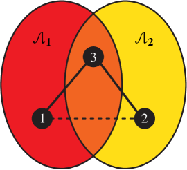
Figure 1: A graphical representation of the dependencies among edges induced by brokerage. Consider two overlapping subpopulations $\mathscr{A}_{1}$ and $\mathscr{A}_{2}$. The nodes $1\in\mathscr{A}_{1}\setminus\,\mathscr{A}_{2}$ and $2\in\mathscr{A}_{2}\setminus\,\mathscr{A}_{1}$ do not belong to the same subpopulation, but the shared partner $3\in\mathscr{A}_{1}\,\cap\,\mathscr{A}_{2}$ in the intersection of subpopulations $\mathscr{A}_{1}$ and $\mathscr{A}_{2}$ can facilitate an edge between nodes $1$ and $2$, indicated by the dashed line between nodes $1$ and $2$.

Define, for each node $i\in\mathscr{N}$, its neighborhood $\mathscr{N}_{i}$ as the subset of all other nodes $j\in\mathscr{N}\setminus\{i\}$ that share at least one subpopulation with node $i\in\mathscr{N}$:

$$\begin{array}[]{lllllllllllll}\mathscr{N}_{i}\;\coloneqq\;\left\{j\in\mathscr{N}\setminus\{i\}:\,\exists\;k\in\{1,\dots,K\}\mbox{ such that }i\in\mathscr{A}_{k}\mbox{ and }j\in\mathscr{A}_{k}\right\}.\end{array}$$

To capture dependence among edges induced by shared partners in the intersections of neighborhoods, we consider functions of edges $\varphi_{i,j}$ of the form

$$\begin{array}[]{lllllllllllll}\varphi_{i,j}(x_{i,j},\,\bm{x}_{\mathscr{S}_{i,j}};\,{\rm Nature})\,\coloneqq\,a_{i,j}(x_{i,j})\,\exp\left((\theta_{i}+\theta_{j})\,x_{i,j}+\theta_{N+1}\,b_{i,j}(x_{i,j},\,\bm{x}_{\mathscr{S}_{i,j}})\right),\end{array}$$

where $\mathscr{S}_{i,j}\subset\mathscr{N}$ is the set of unordered pairs of nodes such that one node is an element of $\{i,\,j\}$ and the other node is an element of $\mathscr{N}_{i}\,\cap\,\mathscr{N}_{j}$,$a_{i,j}(x_{i,j})$ is $1$ if $x_{i,j}\in\{0,1\}$ and is $0$ otherwise, and

$$\begin{array}[]{lllllllllllllllll}b_{i,j}(x_{i,j},\bm{x}_{\mathscr{S}_{i,j}})\coloneqq\begin{cases}0&\mbox{if }\mathscr{N}_{i}\cap\mathscr{N}_{j}=\emptyset\vspace{0.25cm}\\ x_{i,j}\,\mathbbm{1}\left(\displaystyle\sum\limits_{h\in\mathscr{N}_{i}\,\cap\,\mathscr{N}_{j}}x_{i,h}\,x_{j,h}\geq 1\right)&\mbox{if }\mathscr{N}_{i}\cap\mathscr{N}_{j}\neq\emptyset.\end{cases}\end{array}$$ (2.5)

Here, $\mathbbm{1}(\sum_{h\,\in\,\mathscr{N}_{i}\,\cap\,\mathscr{N}_{j}}x_{i,h}\,x_{j,h}\geq 1)$ is an indicator function, which is $1$ if nodes $i$ and $j$ have at least one shared partner in the intersection of neighborhoods $\mathscr{N}_{i}$ and $\mathscr{N}_{j}$ and is $0$ otherwise, and ${\rm Nature}\coloneqq(\theta_{1},\dots,\theta_{N+1})\in\mathbb{R}^{N+1}$.

Remark. Generalized $\beta$-model captures brokerage in networks. The generalized $\beta$-model captures brokerage in networks, along with heterogeneity in the propensities of nodes to form edges. To demonstrate, consider the two overlapping subpopulations $\mathscr{A}_{1}$ and $\mathscr{A}_{2}$ shown in Figure 1. The nodes $1\in\mathscr{A}_{1}\setminus\,\mathscr{A}_{2}$ and $2\in\mathscr{A}_{2}\setminus\,\mathscr{A}_{1}$ do not belong to the same subpopulation, but the shared partner $3\in\mathscr{A}_{1}\,\cap\,\mathscr{A}_{2}$ in the intersection of subpopulations $\mathscr{A}_{1}$ and $\mathscr{A}_{2}$ can facilitate an edge between nodes $1$ and $2$, provided $\theta_{N+1}>0$. In the language of network science, nodes in the intersection $\mathscr{A}_{1}\,\cap\,\mathscr{A}_{2}$ of subpopulations $\mathscr{A}_{1}$ and $\mathscr{A}_{2}$ can act as brokers, facilitating edges between nodes in $\mathscr{A}_{1}\setminus\mathscr{A}_{2}$ and nodes in $\mathscr{A}_{2}\setminus\mathscr{A}_{1}$. In fact, the generalized $\beta$-model can capture an excess in the expected number of brokered edges relative to the $\beta$-model, in the sense that

$$\begin{array}[]{lllllllllllllllll}\begin{array}[]{ccccc}\underbrace{\mathbb{E}_{\theta_{1},\dots,\theta_{N},\theta_{N+1}>0}\;b(\bm{X})}&>&\underbrace{\mathbb{E}_{\theta_{1},\dots,\theta_{N},\theta_{N+1}=0}\;b(\bm{X})},\vspace{0.25cm}\\ \mbox{\em generalized $\beta$-model}&&\mbox{\em$\beta$-model}\end{array}\end{array}$$ (2.6)

where $b(\bm{X})=\sum_{i<j}^{N}\,b_{i,j}(X_{i,j},\,\bm{X}_{\mathscr{S}_{i,j}})$ and $\mathbb{E}_{\theta_{1},\dots,\theta_{N},\theta_{N+1}}\,b(\bm{X})$ is the expectation of $b(\bm{X})$ under $(\theta_{1},\dots,\theta_{N},\theta_{N+1})\in\mathbb{R}^{N+1}$. In other words, the generalized $\beta$-model with $\theta_{N+1}>0$ generates graphs that have, on average, more brokered edges than the $\beta$-model, assuming that the propensities $\theta_{1},\dots,\theta_{N}$ of nodes $1,\dots,N$ to form edges are the same under both models. The inequality in (2.6) follows from the fact that the generalized $\beta$-model is an exponential-family model along with Corollary 2.5 of Brown [5, p. 37].

2.4 Model 3: sparse generalized $\beta$-models with dependent edges

Sparse random graphs have been studied since the pioneering work of Erdős and Rényi [e.g., 33, 28, 29, 11]. To develop sparse versions of generalized $\beta$-models, it makes sense to penalize edges between nodes $i\in\mathscr{N}$ and $j\in\mathscr{N}$ that are distant in the sense that $\mathscr{N}_{i}\,\cap\,\mathscr{N}_{j}=\emptyset$, without penalizing edges between nodes that are close in the sense that $\mathscr{N}_{i}\,\cap\,\mathscr{N}_{j}\neq\emptyset$. We therefore induce sparsity by considering Model 2 with

$$\begin{array}[]{lllllllllllll}a_{i,j}(x_{i,j})&\coloneqq&\begin{cases}N^{-\alpha\;x_{i,j}\,\mathbbm{1}(\mathscr{N}_{i}\,\cap\,\mathscr{N}_{j}=\emptyset)}&\mbox{ if }x_{i,j}\in\{0,1\}\vspace{0.25cm}\\ 0&\mbox{ otherwise,}\end{cases}\end{array}$$

where $\alpha\in(0,\,1]$ is called the level of sparsity of the random graph.

To demonstrate that Model 3 encourages random graphs to be sparse, we bound the expected degrees of nodes.

Proposition 2.1.

Consider Model 3 with ${\rm Nature}\in\mathbb{R}^{N+1}$ and $\alpha\in(0,1]$. Then

$$\begin{array}[]{lllllllllllll}\max\limits_{1\leq i\leq N}\,\mathbb{E}_{{\rm Nature}}\left(\displaystyle\sum\limits_{j\neq i}^{N}\,X_{i,j}\right)\;\leq\;2\;\exp(3\,|\!|{\rm Nature}|\!|_{\infty})\;\left(\left(\max\limits_{1\leq h\leq N}|\mathscr{N}_{h}|\right)^{2}+N^{1-\alpha}\right).\end{array}$$

Proposition 2.1 reveals that when the neighborhoods $\mathscr{N}_{h}$ of nodes $h\in\mathscr{N}$ are not too large, the random graph is sparse in the sense that the expected degrees of all nodes are $o(N)$. For example, if $\max_{1\leq h\leq N}|\mathscr{N}_{h}|$ and $|\!|{\rm Nature}|\!|_{\infty}$ are bounded above, the expected degrees of nodes are $O(N^{1-\alpha})$.

3 Statistical guarantees

We establish consistency results and convergence rates of maximum likelihood and pseudo-likelihood-based $M$-estimators in Sections 3.2 and 3.3, respectively. We then present applications to $\beta$- and generalized $\beta$-models with dependent edges in Section 3.4. To prepare the ground, we first discuss how the dependence among edges and the smoothness of sufficient statistics can be quantified. To ease the presentation, we replace the double subscripts of edge variables by single subscripts and write $(X_{m})_{1\leq m\leq M}$ instead of $(X_{i,j})_{i<j:\,i\in\mathscr{N},\,j\in\mathscr{N}}$, where $M\coloneqq\binom{N}{2}$. The data-generating parameter vector is denoted by ${\rm Nature}^{\star}\in\bm{\Theta}=\mathbb{R}^{p}$.

3.1 Controlling dependence and smoothness

To obtain consistency results and convergence rates based on a single observation of a random graph with dependent edges, we need to control the dependence among edges along with the smoothness of the sufficient statistics of the model.

The dependence among edges can be controlled by bounding the total variation distance between conditional probability mass functions of edge variables, quantifying how much the conditional probability mass functions of edge variables are affected by changes of other edge variables. Define $\bm{X}_{a:b}\coloneqq(X_{a},\dots,X_{b})\in\{0,\,1\}^{b-a+1}$, where $a\leq b$ and $a,\,b\in\{1,\ldots,M\}$. For each $i\in\{1,\dots,M\}$, we denote the conditional probability mass function of subgraph $\bm{X}_{i+1:M}$ given subgraph $(\bm{X}_{1:i-1},\,X_{i})=(\bm{x}_{1:i-1},\,x_{i})$ by $\mathbb{P}_{{\rm Nature}^{\star},\bm{x}_{1:i-1},x_{i}}$:

$$\begin{array}[]{lllllllllllll}\mathbb{P}_{{\rm Nature}^{\star},\bm{x}_{1:i-1},x_{i}}(\bm{X}_{i+1:M}=\bm{a})\,\coloneqq\,\mathbb{P}_{{\rm Nature}^{\star}}(\bm{X}_{i+1:M}=\bm{a}\mid(\bm{X}_{1:i-1},X_{i})=(\bm{x}_{1:i-1},x_{i})),\end{array}$$

where $\bm{a}\in\{0,1\}^{M-i}$. We quantify the dependence among edges by bounding the total variation distance between the conditional probability mass functions $\mathbb{P}_{{\rm Nature}^{\star},\bm{x}_{1:i-1},0}$  and $\mathbb{P}_{{\rm Nature}^{\star},\bm{x}_{1:i-1},1}$  by using coupling methods [27]:

$$\begin{array}[]{lllllllllllll}|\!|\mathbb{P}_{{\rm Nature}^{\star},\bm{x}_{1:i-1},0}-\mathbb{P}_{{\rm Nature}^{\star},\bm{x}_{1:i-1},1}|\!|_{{\tiny\mbox{TV}}}\;\leq\;\mathbb{Q}_{{\rm Nature}^{\star},i,\bm{x}_{1:i-1}}(\bm{X}^{\star}_{i+1:M}\neq\bm{X}^{\star\star}_{i+1:M}),\end{array}$$

where the pair of random vectors $(\bm{X}^{\star}_{i+1:M},\bm{X}^{\star\star}_{i+1:M})\in\{0,1\}^{M-i}\times\{0,1\}^{M-i}$ with joint probability mass function $\mathbb{Q}_{{\rm Nature}^{\star},i,\bm{x}_{1:i-1}}$ is a coupling of  $\mathbb{P}_{{\rm Nature}^{\star},\bm{x}_{1:i-1},0}$  and $\mathbb{P}_{{\rm Nature}^{\star},\bm{x}_{1:i-1},1}$ [27]. The coupling $\mathbb{Q}_{{\rm Nature}^{\star},i,\bm{x}_{1:i-1}}$ is constructed in Lemma C.20 in the supplement [38]. Based on the coupling $\mathbb{Q}_{{\rm Nature}^{\star},i,\bm{x}_{1:i-1}}$, we quantify the dependence among edges by the spectral norm $|\!|\!|\mathscr{D}_{N}({\rm Nature}^{\star})|\!|\!|_{2}$ of the upper triangular $M\times M$ coupling matrix $\mathscr{D}_{N}({\rm Nature}^{\star})$ with elements

$$\begin{array}[]{lllllllllllll}\mathscr{D}_{i,j}({\rm Nature}^{\star})&\coloneqq&\begin{cases}0&\mbox{ if }j<i\\ 1&\mbox{ if }j=i\\ \max\limits_{\bm{x}_{1:i-1}\in\{0,1\}^{i-1}}\mathbb{Q}_{{\rm Nature}^{\star},i,\bm{x}_{1:i-1}}(X_{j}^{\star}\neq X_{j}^{\star\star})&\mbox{ if }j>i.\end{cases}\end{array}$$

While the definition of $\mathscr{D}_{N}({\rm Nature}^{\star})$ depends on the ordering of edge variables, it is possible to obtain bounds on the spectral norm $|\!|\!|\mathscr{D}_{N}({\rm Nature}^{\star})|\!|\!|_{2}$ of $\mathscr{D}_{N}({\rm Nature}^{\star})$ that hold for all orderings. We describe in Section 3.3.2 how $|\!|\!|\mathscr{D}_{N}({\rm Nature}^{\star})|\!|\!|_{2}$ can be bounded by using coupling methods from percolation theory [39].

To control the smoothness of the sufficient statistics of the model, define

$$\begin{array}[]{lllllllllllll}\Xi_{i,j}&\coloneqq&\max\limits_{(\bm{x},\,\bm{x}^{\prime})\,\in\,\mathbb{X}\times\mathbb{X}:\;\;x_{k}=x_{k}^{\prime}\mbox{\footnotesize\, for all }k\neq j}\;|s_{i}(\bm{x})-s_{i}(\bm{x}^{\prime})|,&j=1,\dots,M,\end{array}$$

where $s_{1}(\bm{x}),\dots,s_{p}(\bm{x})$ are the coordinates of the sufficient statistic vector $s(\bm{x})\in\mathbb{R}^{p}$ defined in (2.4). Let $\bm{\Xi}_{i}=(\Xi_{i,1},\dots,\Xi_{i,M})$ and define

$$\begin{array}[]{lllllllllllll}\Psi_{N}&\coloneqq&\max\limits_{1\leq i\leq p}\,|\!|\bm{\Xi}_{i}|\!|_{2}.\end{array}$$

To exclude the trivial case where $\Psi_{N}=0$, we assume that there exists an integer $N_{0}\geq 3$ such that $\Psi_{N}>0$ for all $N>N_{0}$.

3.2 Maximum likelihood estimators

Consider a single observation $\bm{x}$ of a random graph $\bm{X}$ with dependent edges. Let $\ell({\rm Nature};\,\bm{x})\coloneqq\log f_{{\rm Nature}}(\bm{x})$ and

$$\begin{array}[]{lllllllllllll}\widehat{\bm{\Theta}}&\coloneqq&\left\{{\rm Nature}\,\in\,\mathbb{R}^{p}:\;|\!|\nabla_{{\rm Nature}}\;\ell({\rm Nature};\,\bm{x})|\!|_{\infty}\,=\,0\,\right\}.\end{array}$$

We develop a novel approach to establishing consistency results and convergence rates of maximum likelihood estimators for discrete undirected graphical models with exponential parameterizations and parameter vectors of increasing dimension in single-observation scenarios. These results serve as a stepping stone for establishing consistency results and convergence rates of pseudo-likelihood-based $M$-estimators in Section 3.3.

Let $\mathcal{I}({\rm Nature})\coloneqq\nabla_{{\rm Nature}}^{2}\,\psi({\rm Nature})=\mathbb{C}_{{\rm Nature}}\,s(\bm{X})=-\mathbb{E}_{{\rm Nature}}\,\nabla_{{\rm Nature}}^{2}\,\,\ell({\rm Nature};\,\bm{X})$ [26, Theorem 2.7.1, p. 49]. Assume that there exists a constant $\epsilon^{\star}\in(0,\,\infty)$, independent of $N$ and $p$, such that $\mathcal{I}({\rm Nature})$ is invertible for all ${\rm Nature}\in\mathscr{B}_{\infty}({\rm Nature}^{\star},\,\epsilon^{\star})$. Define

$$\begin{array}[]{lllllllllllllllll}\Lambda_{N}({\rm Nature}^{\star})&\coloneqq&\sup\limits_{{\rm Nature}\,\in\,\mathscr{B}_{\infty}({\rm Nature}^{\star},\,\epsilon^{\star})}\,|\!|\!|\mathcal{I}({\rm Nature})^{-1}|\!|\!|_{\infty}\vspace{0.25cm}\\ \Phi_{N}({\rm Nature}^{\star})&\coloneqq&\Lambda_{N}({\rm Nature}^{\star})\,|\!|\!|\mathscr{D}_{N}({\rm Nature}^{\star})|\!|\!|_{2}\,\Psi_{N}\,\sqrt{\log\,\max\{N,p\}}.\end{array}$$ (3.1)

Theorem 3.2.

Consider a single observation of a random graph with $N$ nodes and dependent edges. Assume that ${\rm Nature}^{\star}\in\bm{\Theta}=\mathbb{R}^{p}$, where $p\to\infty$ as $N\to\infty$ is allowed. If  $\Phi_{N}({\rm Nature}^{\star})\to 0$ as $N\to\infty$, there exists an integer $N_{0}\geq 3$ such that, for all $N>N_{0}$, the random set $\widehat{\bm{\Theta}}$ is non-empty and its unique element $\widehat{\bm{\theta}}$ satisfies

$$\begin{array}[]{lllllllllllll}|\!|\widehat{\bm{\theta}}-{\rm Nature}^{\star}|\!|_{\infty}&\leq&\sqrt{3/2}\;\,\Phi_{N}({\rm Nature}^{\star})\end{array}$$

with probability at least $1-2\,/\max\{N,\,p\}^{2}$.

While Theorem 3.2 is stated in terms of random graphs, Theorem 3.2 covers discrete undirected graphical models with exponential parameterizations and parameter vectors of increasing dimension in single-observation scenarios. Theorem 3.2 suggests that the convergence rate of maximum likelihood estimators depends on the dimension $p$ of the parameter space $\bm{\Theta}=\mathbb{R}^{p}$ and

• the inverse Fisher information matrix in a neighborhood of the data-generating parameter vector ${\rm Nature}^{\star}\in\mathbb{R}^{p}$, quantified by $\Lambda_{N}({\rm Nature}^{\star})$;

• the dependence induced by the model, quantified by $|\!|\!|\mathscr{D}_{N}({\rm Nature}^{\star})|\!|\!|_{2}$;

• the sensitivity of sufficient statistics, quantified by $\Psi_{N}$.

We highlight the impact of two complex phenomena on the convergence rate: phase transitions and model near-degeneracy [19, 32, 35, 8, 36]. It is known that some random graph models with dependent edges [e.g., the ill-posed edge-and-triangle model, 19, 32, 35, 8, 36] exhibit phase transitions and model near-degeneracy. To examine the impact of phase transitions and model near-degeneracy on the convergence rate, consider a model with a parameter space $\bm{\Theta}=\mathbb{R}^{p}$ divided into two or more subsets (regimes) inducing very different distributions, some of which may place almost all mass on a small subset of graphs (e.g., near-empty or near-complete graphs).

Phase transitions. On subsets of $\bm{\Theta}$ where transitions between such regimes occur, small changes of natural parameters ${\rm Nature}$ can lead to large changes of mean-value parameters $\bm{\mu}({\rm Nature})\coloneqq\nabla_{{\rm Nature}}\,\psi({\rm Nature})=\mathbb{E}_{{\rm Nature}}\,s(\bm{X})$. In such cases, $\mathcal{I}({\rm Nature})\coloneqq\nabla_{{\rm Nature}}^{2}\,\,\psi({\rm Nature})$ can become ill-posed and non-invertible, in which case Theorem 3.2 does not establish consistency.

Model near-degeneracy. On subsets of $\bm{\Theta}$ inducing near-degenerate distributions, the variances of sufficient statistics (e.g., the number of edges) can be small, so that the elements on the main diagonal of  $\mathcal{I}({\rm Nature})=\mathbb{C}_{{\rm Nature}}\,s(\bm{X})$ can be small for some or all ${\rm Nature}\,\in\,\mathscr{B}_{\infty}({\rm Nature}^{\star},\,\epsilon^{\star})$. In such cases, the convergence rate is reduced via $\Lambda_{N}({\rm Nature}^{\star})$. In addition, model near-degeneracy is sometimes associated with strong dependence and high sensitivity of sufficient statistics [35], depressing the convergence rate via $|\!|\!|\mathscr{D}_{N}({\rm Nature}^{\star})|\!|\!|_{2}$ and $\Psi_{N}$. An example is the ill-posed edge-and-triangle model [19, 32, 35, 8, 36]. We are interested in well-posed models that are amenable to scalable estimation with statistical guarantees. Therefore, the applications in Section 3.4 focus on models that leverage additional structure to control all relevant quantities.

Proof of Theorem 3.2. Let $\bm{\mu}({\rm Nature})\coloneqq\mathbb{E}_{{\rm Nature}}\,s(\bm{X})$ be the mean-value parameter vector of the exponential family (2.3) parameterized by (2.1) and (2.2). The map $\bm{\mu}:\bm{\Theta}\mapsto\mathbb{M}$ from the natural parameter space $\bm{\Theta}\coloneqq\{{\rm Nature}\in\mathbb{R}^{p}:\,\psi({\rm Nature})<\infty\}=\mathbb{R}^{p}$ to the mean-value parameter space $\mathbb{M}\,\coloneqq\,\bm{\mu}(\bm{\Theta})$ is a homeomorphism [5, Theorem 3.6, p. 74]. As a result, the inverse map $\bm{\mu}^{-1}:\mathbb{M}\mapsto\bm{\Theta}$ exists and $\bm{\mu}$ and $\bm{\mu}^{-1}$ are continuous, one-to-one, and onto.

By assumption, there exists a constant $\epsilon^{\star}\in(0,\,\infty)$, independent of $N$ and $p$, such that $\mathcal{I}({\rm Nature})$ is invertible for all ${\rm Nature}\in\mathscr{B}_{\infty}({\rm Nature}^{\star},\,\epsilon^{\star})$. The proof of Theorem 3.2 will focus on the subset $\mathscr{B}_{\infty}({\rm Nature}^{\star},\,\epsilon^{\star})$ of $\bm{\Theta}$. We will show in (3.12) that it is legitimate to focus on $\mathscr{B}_{\infty}({\rm Nature}^{\star},\,\epsilon^{\star})$, because the event $\widehat{\bm{\theta}}\,\in\,\mathscr{B}_{\infty}({\rm Nature}^{\star},\,\epsilon^{\star})$ occurs with probability at least $1-2\,/\max\{N,\,p\}^{2}$ for all large enough $N$.

Consider any $\epsilon\in(0,\,\epsilon^{\star})$ and define

$$\begin{array}[]{lllllllllllll}\delta(\epsilon)&\coloneqq&\sup\left\{\rho\,\in\,(0,\,\infty):\,\mathscr{B}_{\infty}(\bm{\mu}({\rm Nature}^{\star}),\,\rho)\;\subseteq\;\bm{\mu}(\mathscr{B}_{\infty}({\rm Nature}^{\star},\,\epsilon))\right\}.\end{array}$$

By definition of $\delta(\epsilon)$, the hypercube $\mathscr{B}_{\infty}(\bm{\mu}({\rm Nature}^{\star}),\,\delta(\epsilon))$ is the largest hypercube centered at $\bm{\mu}({\rm Nature}^{\star})$ and contained in the image $\bm{\mu}(\mathscr{B}_{\infty}({\rm Nature}^{\star},\,\epsilon))$ of  $\mathscr{B}_{\infty}({\rm Nature}^{\star},\,\epsilon)$. As a result, $\delta(\epsilon)$ is the greatest real number $\rho\in(0,\,\infty)$ with the property that every element $\bm{\mu}({\rm Nature})\in\mathscr{B}_{\infty}(\bm{\mu}({\rm Nature}^{\star}),\,\rho)$ pulls back to an element ${\rm Nature}\in\mathscr{B}_{\infty}({\rm Nature}^{\star},\,\epsilon)$:

$$\begin{array}[]{lllllllllllllllll}\delta(\epsilon)&=&\sup\left\{\rho\,\in\,(0,\,\infty):\,\bm{\mu}^{-1}\left(\mathscr{B}_{\infty}(\bm{\mu}({\rm Nature}^{\star}),\,\rho)\right)\,\subseteq\,\mathscr{B}_{\infty}({\rm Nature}^{\star},\,\epsilon)\right\}.\end{array}$$ (3.2)

A direct consequence of (3.2) is the following observation:

$$\begin{array}[]{c}\mbox{If }\rho\,\in\,(0,\,\infty)\mbox{ satisfies }\bm{\mu}^{-1}\left(\mathscr{B}_{\infty}(\bm{\mu}({\rm Nature}^{\star}),\,\rho)\right)\;\subseteq\;\mathscr{B}_{\infty}({\rm Nature}^{\star},\,\epsilon),\vspace{0.25cm}\\ \mbox{then }\rho\;\leq\;\delta(\epsilon).\end{array}$$ (3.3)

The observation (3.3) paves the way for establishing convergence rates for $\widehat{\bm{\theta}}$ based on $\bm{\mu}(\widehat{\bm{\theta}})$, because we will prove that

$$\begin{array}[]{lllllllllllllllll}\bm{\mu}^{-1}\left(\mathscr{B}_{\infty}\left(\bm{\mu}({\rm Nature}^{\star}),\,\dfrac{\epsilon}{\Lambda_{N}({\rm Nature}^{\star})}\right)\right)&\subseteq&\mathscr{B}_{\infty}({\rm Nature}^{\star},\,\epsilon),\end{array}$$ (3.4)

which will establish the following fundamental relation between $\epsilon$ and $\delta(\epsilon)$:

$$\begin{array}[]{lllllllllllllllll}\dfrac{\epsilon}{\Lambda_{N}({\rm Nature}^{\star})}&\leq&\delta(\epsilon).\end{array}$$ (3.5)

To prove (3.4) and (3.5) and establish convergence rates for $\widehat{\bm{\theta}}$ based on $\bm{\mu}(\widehat{\bm{\theta}})$, note that $\mathscr{B}_{\infty}({\rm Nature}^{\star},\,\epsilon)\subset\bm{\Theta}=\mathbb{R}^{p}$ implies $\bm{\mu}(\mathscr{B}_{\infty}({\rm Nature}^{\star},\,\epsilon))\subset\mathbb{M}$ and that the random set $\widehat{\bm{\Theta}}$ is non-empty in the event $s(\bm{X})\,\in\,\bm{\mu}(\mathscr{B}_{\infty}({\rm Nature}^{\star},\,\epsilon))\subset\mathbb{M}$, with its unique element $\widehat{\bm{\theta}}\in\widehat{\bm{\Theta}}$ solving $\bm{\mu}(\widehat{\bm{\theta}})=s(\bm{X})$ [5, Theorem 5.5, p. 148]. We can thus bound the probability of event $\widehat{\bm{\theta}}\in\mathscr{B}_{\infty}({\rm Nature}^{\star},\,\epsilon)$ as follows:

$$\begin{array}[]{lllllllllllllllll}\mathbb{P}(\widehat{\bm{\theta}}\in\mathscr{B}_{\infty}({\rm Nature}^{\star},\,\epsilon))&=&\mathbb{P}(\bm{\mu}(\widehat{\bm{\theta}})\in\bm{\mu}(\mathscr{B}_{\infty}({\rm Nature}^{\star},\,\epsilon)))\vspace{0.25cm}\\ &\geq&\mathbb{P}(\bm{\mu}(\widehat{\bm{\theta}})\in\mathscr{B}_{\infty}(\bm{\mu}({\rm Nature}^{\star}),\,\delta(\epsilon)))\vspace{.15cm}\\ &\geq&1-2\,\exp\left(-\dfrac{2\;\delta(\epsilon)^{2}}{|\!|\!|\mathscr{D}_{N}({\rm Nature}^{\star})|\!|\!|_{2}^{2}\;\Psi_{N}^{2}}+\log p\right),\end{array}$$ (3.6)

where the first line follows from the fact that $\bm{\mu}:\bm{\Theta}\mapsto\mathbb{M}$ is a homeomorphism and $\widehat{\bm{\theta}}$ exists, is unique, and solves $\bm{\mu}(\widehat{\bm{\theta}})=s(\bm{X})$ in the event $s(\bm{X})\in\bm{\mu}(\mathscr{B}_{\infty}({\rm Nature}^{\star},\,\epsilon))\subset\mathbb{M}$ [5, Theorem 5.5, p. 148], the second line follows from $\mathscr{B}_{\infty}(\bm{\mu}({\rm Nature}^{\star}),\,\delta(\epsilon))\,\subseteq\,\bm{\mu}(\mathscr{B}_{\infty}({\rm Nature}^{\star},\,\epsilon))$, and the third line follows from $\bm{\mu}(\widehat{\bm{\theta}})=s(\bm{X})$ along with Lemma A.7 in the supplement [38].

We bound the right-hand side of (3.6) by bounding $\delta(\epsilon)$, taking advantage of observation (3.3). Consider any $\rho\leq\delta(\epsilon)$ and any $\bm{\mu}^{\prime}\in\mathscr{B}_{\infty}(\bm{\mu}({\rm Nature}^{\star}),\,\rho)$. The assumption $\rho\leq\delta(\epsilon)$, together with the definition of $\delta(\epsilon)$, implies that

$$\begin{array}[]{lllllllllllll}\bm{\mu}^{\prime}&\in&\mathscr{B}_{\infty}(\bm{\mu}({\rm Nature}^{\star}),\,\rho)&\subseteq&\mathscr{B}_{\infty}(\bm{\mu}({\rm Nature}^{\star}),\,\delta(\epsilon))&\subseteq&\bm{\mu}(\mathscr{B}_{\infty}({\rm Nature}^{\star},\,\epsilon)).\end{array}$$

Therefore, the natural parameter vector ${\rm Nature}^{\prime}\coloneqq\bm{\mu}^{-1}(\bm{\mu}^{\prime})$ corresponding to the mean-value parameter vector $\bm{\mu}^{\prime}$ falls into $\mathscr{B}_{\infty}({\rm Nature}^{\star},\,\epsilon)$:

$$\begin{array}[]{lllllllllllll}{\rm Nature}^{\prime}&\in&\bm{\mu}^{-1}(\mathscr{B}_{\infty}(\bm{\mu}({\rm Nature}^{\star}),\,\rho))&\subseteq&\bm{\mu}^{-1}(\mathscr{B}_{\infty}(\bm{\mu}({\rm Nature}^{\star}),\,\delta(\epsilon)))&\subseteq&\mathscr{B}_{\infty}({\rm Nature}^{\star},\,\epsilon).\end{array}$$

In addition, ${\rm Nature}^{\prime}$ falls into $\mathscr{B}_{\infty}({\rm Nature}^{\star},\,\epsilon^{\star})$, because $\epsilon\in(0,\,\epsilon^{\star})$:

$$\begin{array}[]{lllllllllllll}{\rm Nature}^{\prime}&\in&\mathscr{B}_{\infty}({\rm Nature}^{\star},\,\epsilon)&\subset&\mathscr{B}_{\infty}({\rm Nature}^{\star},\,\epsilon^{\star}).\end{array}$$

By the multivariate mean-value theorem [16, Theorem 5], there exists

$$\begin{array}[]{lllllllllllll}{\rm Nature}^{\prime\prime}&\coloneqq&\lambda\,{\rm Nature}^{\star}+(1-\lambda)\,{\rm Nature}^{\prime}&\in&\mathscr{B}_{\infty}({\rm Nature}^{\star},\,\epsilon^{\star}),&\lambda\in(0,1)\end{array}$$

such that

$$\begin{array}[]{lllllllllllll}\bm{\mu}({\rm Nature}^{\prime})-\bm{\mu}({\rm Nature}^{\star})&=&\mathcal{I}({\rm Nature}^{\prime\prime})\,({\rm Nature}^{\prime}-{\rm Nature}^{\star}).\end{array}$$

By assumption, $\mathcal{I}({\rm Nature})$ is invertible for all ${\rm Nature}\in\mathscr{B}_{\infty}({\rm Nature}^{\star},\,\epsilon^{\star})$, which includes ${\rm Nature}^{\prime\prime}\in\mathscr{B}_{\infty}({\rm Nature}^{\star},\,\epsilon^{\star})$. As a result, ${\rm Nature}^{\prime}-{\rm Nature}^{\star}=\mathcal{I}({\rm Nature}^{\prime\prime})^{-1}\,(\bm{\mu}({\rm Nature}^{\prime})-\bm{\mu}({\rm Nature}^{\star}))$ and

$$\begin{array}[]{lllllllllllllllll}|\!|{\rm Nature}^{\prime}-{\rm Nature}^{\star}|\!|_{\infty}&\leq&|\!|\!|\mathcal{I}({\rm Nature}^{\prime\prime})^{-1}|\!|\!|_{\infty}\,|\!|\bm{\mu}({\rm Nature}^{\prime})-\bm{\mu}({\rm Nature}^{\star})|\!|_{\infty}\;<\;\rho\;|\!|\!|\mathcal{I}({\rm Nature}^{\prime\prime})^{-1}|\!|\!|_{\infty},\end{array}$$ (3.7)

recalling that $|\!|\bm{\mu}({\rm Nature}^{\prime})-\bm{\mu}({\rm Nature}^{\star})|\!|_{\infty}<\rho$  for all  $\bm{\mu}({\rm Nature}^{\prime})\in\mathscr{B}_{\infty}(\bm{\mu}({\rm Nature}^{\star}),\,\rho)$; note that $\bm{\mu}({\rm Nature}^{\prime})$ is identical to $\bm{\mu}^{\prime}\in\mathscr{B}_{\infty}(\bm{\mu}({\rm Nature}^{\star}),\,\rho)$. As a consequence, all $\rho\in(0,\infty)$ satisfying $\rho\leq\epsilon\,/\,|\!|\!|\mathcal{I}({\rm Nature}^{\prime\prime})^{-1}|\!|\!|_{\infty}$ guarantee that $|\!|{\rm Nature}^{\prime}-{\rm Nature}^{\star}|\!|_{\infty}<\epsilon$. Choosing $\rho\coloneqq\epsilon\,/\,\Lambda_{N}({\rm Nature}^{\star})$ with $\Lambda_{N}({\rm Nature}^{\star})\coloneqq\sup_{{\rm Nature}\,\in\,\mathscr{B}_{\infty}({\rm Nature}^{\star},\,\epsilon^{\star})}\,|\!|\!|\mathcal{I}({\rm Nature})^{-1}|\!|\!|_{\infty}$ and applying (3.7) with the chosen $\rho$ establishes the fundamental relation

$$\begin{array}[]{lllllllllllllllll}\bm{\mu}^{-1}\left(\mathscr{B}_{\infty}\left(\bm{\mu}({\rm Nature}^{\star}),\,\dfrac{\epsilon}{\Lambda_{N}({\rm Nature}^{\star})}\right)\right)&\subseteq&\mathscr{B}_{\infty}({\rm Nature}^{\star},\,\epsilon).\end{array}$$ (3.8)

The fundamental relation (3.8), combined with the observation (3.3), implies that $\epsilon$ is related to $\delta(\epsilon)$ as follows:

$$\begin{array}[]{lllllllllllllllll}\dfrac{\epsilon}{\Lambda_{N}({\rm Nature}^{\star})}&\leq&\delta(\epsilon).\end{array}$$ (3.9)

Armed with inequality (3.9), we revisit (3.6) to obtain

$$\begin{array}[]{lllllllllllll}\mathbb{P}(\widehat{\bm{\theta}}\in\mathscr{B}_{\infty}({\rm Nature}^{\star},\,\epsilon))&\geq&1-2\,\exp\left(-\dfrac{2\,\delta(\epsilon)^{2}}{|\!|\!|\mathscr{D}_{N}({\rm Nature}^{\star})|\!|\!|_{2}^{2}\,\Psi_{N}^{2}}+\log\,p\right)\vspace{0.25cm}\\ &\geq&1-2\,\exp\left(-\dfrac{2\,\epsilon^{2}}{\Lambda_{N}({\rm Nature}^{\star})^{2}\,|\!|\!|\mathscr{D}_{N}({\rm Nature}^{\star})|\!|\!|_{2}^{2}\,\Psi_{N}^{2}}+\log\,p\right).\end{array}$$

Choosing $\epsilon\,\coloneqq\,\sqrt{3/2}\;\,\Phi_{N}({\rm Nature}^{\star})$ establishes

$$\begin{array}[]{lllllllllllllllll}\mathbb{P}(\widehat{\bm{\theta}}\,\in\,\mathscr{B}_{\infty}({\rm Nature}^{\star},\sqrt{3/2}\;\Phi_{N}({\rm Nature}^{\star})))&\geq&1-\dfrac{2}{\max\{N,\,p\}^{2}}.\end{array}$$ (3.10)

To complete the proof, we show that the focus on the subset $\mathscr{B}_{\infty}({\rm Nature}^{\star},\,\epsilon^{\star})$ of $\bm{\Theta}$ is legitimate, by noting that the assumption $\Phi_{N}({\rm Nature}^{\star})\to 0$ as $N\to\infty$ implies that there exists an integer $N_{0}\geq 3$ such that $\epsilon\coloneqq\sqrt{3/2}\;\,\Phi_{N}({\rm Nature}^{\star})<\epsilon^{\star}$ for all $N>N_{0}$. The fact that $\sqrt{3/2}\;\Phi_{N}({\rm Nature}^{\star})<\epsilon^{\star}$ for all $N>N_{0}$ implies

$$\begin{array}[]{lllllllllllllllll}\mathscr{B}_{\infty}({\rm Nature}^{\star},\sqrt{3/2}\;\Phi_{N}({\rm Nature}^{\star}))&\subset&\mathscr{B}_{\infty}({\rm Nature}^{\star},\,\epsilon^{\star})&\mbox{for all}&N>N_{0}.\end{array}$$ (3.11)

The relation (3.11), along with the lower bound on the probability of event $\widehat{\bm{\theta}}\in\mathscr{B}_{\infty}({\rm Nature}^{\star},\sqrt{3/2}\;\Phi_{N}({\rm Nature}^{\star}))$ in (3.10), shows that

$$\begin{array}[]{lllllllllllllllll}\mathbb{P}(\widehat{\bm{\theta}}\in\mathscr{B}_{\infty}({\rm Nature}^{\star},\,\epsilon^{\star}))&\geq&\mathbb{P}(\widehat{\bm{\theta}}\,\in\,\mathscr{B}_{\infty}({\rm Nature}^{\star},\sqrt{3/2}\;\Phi_{N}({\rm Nature}^{\star})))\vspace{0.25cm}\\ &\geq&1-\dfrac{2}{\max\{N,\,p\}^{2}}\;\mbox{ for all }\;N>N_{0}.\end{array}$$ (3.12)

We conclude that, for all $N>N_{0}$, the random set $\widehat{\bm{\Theta}}$ is non-empty and its unique element $\widehat{\bm{\theta}}$ satisfies

$$\begin{array}[]{lllllllllllll}|\!|\widehat{\bm{\theta}}-{\rm Nature}^{\star}|\!|_{\infty}&\leq&\sqrt{3/2}\;\,\Phi_{N}({\rm Nature}^{\star})\end{array}$$

with probability at least $1-2\,/\max\{N,\,p\}^{2}$. ∎

3.3 Pseudo-likelihood-based $M$-estimators

Maximum likelihood estimators are unappealing on computational grounds, because evaluating $\ell({\rm Nature};\,\bm{x})$ requires evaluating the normalizing constant of $f_{{\rm Nature}}(\bm{x})$. The normalizing constant of $f_{{\rm Nature}}(\bm{x})$ is a sum over $\exp(M\log 2)$ possible graphs and cannot be computed unless $M\coloneqq\binom{N}{2}$ is small or the model makes restrictive independence assumptions. As a scalable alternative, consider $M$-estimators

$$\begin{array}[]{lllllllllllll}\widetilde{\bm{\Theta}}(\gamma_{N})&\coloneqq&\left\{{\rm Nature}\,\in\,\mathbb{R}^{p}:\;|\!|\nabla_{{\rm Nature}}\;\widetilde{\ell}({\rm Nature};\,\bm{x})|\!|_{\infty}\;\leq\;\gamma_{N}\right\},&&\gamma_{N}\in[0,\,\infty)\end{array}$$

based on the pseudo-loglikelihood function

$$\begin{array}[]{lllllllllllll}\widetilde{\ell}({\rm Nature};\,\bm{x})&\coloneqq&\log\displaystyle\prod\limits_{i=1}^{M}f_{{\rm Nature}}(x_{i}\mid\bm{x}_{-i}),\end{array}$$

where $f_{{\rm Nature}}(x_{i}\mid\bm{x}_{-i})$ is the conditional probability of $X_{i}=x_{i}$ given all other edge variables $\bm{X}_{-i}=\bm{x}_{-i}$ ($i=1,\dots,M$).

To bound the statistical error of pseudo-likelihood-based $M$-estimators in single-observation scenarios with $p\to\infty$ parameters, let $i\in\{1,\dots,M\}$ and $\mathfrak{N}_{i}\;\subseteq\;\{1,\dots,M\}\,\setminus\,\{i\}$ be the smallest subset of $\{1,\dots,M\}\,\setminus\,\{i\}$ such that

$$\begin{array}[]{lllllllllllll}X_{i}&\mathchoice{\mathrel{\hbox to0.0pt{$\displaystyle\perp$\hss}\mkern 2.0mu{\displaystyle\perp}}}{\mathrel{\hbox to0.0pt{$\textstyle\perp$\hss}\mkern 2.0mu{\textstyle\perp}}}{\mathrel{\hbox to0.0pt{$\scriptstyle\perp$\hss}\mkern 2.0mu{\scriptstyle\perp}}}{\mathrel{\hbox to0.0pt{$\scriptscriptstyle\perp$\hss}\mkern 2.0mu{\scriptscriptstyle\perp}}}&\bm{X}_{\{1,\dots,M\}\,\setminus\,(\{i\}\,\cup\,\mathfrak{N}_{i})}\mid\bm{X}_{\mathfrak{N}_{i}}.\end{array}$$

Let $\epsilon^{\star}\in(0,\,\infty)$ be a constant, independent of $N$ and $p$, and assume that $-\mathbb{E}\;\nabla_{{\rm Nature}}^{2}\;\widetilde{\ell}({\rm Nature};\bm{X})$ is invertible for all ${\rm Nature}\in\mathscr{B}_{\infty}({\rm Nature}^{\star},\,\epsilon^{\star})$. Define

$$\begin{array}[]{lllllllllllll}\widetilde{\Lambda}_{N}({\rm Nature}^{\star})&\coloneqq&\sup\limits_{{\rm Nature}\,\in\,\mathscr{B}_{\infty}({\rm Nature}^{\star},\,\epsilon^{\star})}|\!|\!|(-\mathbb{E}\;\nabla_{{\rm Nature}}^{2}\;\,\widetilde{\ell}({\rm Nature};\bm{X}))^{-1}|\!|\!|_{\infty}\vspace{0.25cm}\\ \widetilde{\Phi}_{N}({\rm Nature}^{\star})&\coloneqq&\widetilde{\Lambda}_{N}({\rm Nature}^{\star})\,\,(1+D_{N})\,\,|\!|\!|\mathscr{D}_{N}({\rm Nature}^{\star})|\!|\!|_{2}\,\,\Psi_{N}\;\sqrt{\log\max\{N,\,p\}},\end{array}$$

where $D_{N}\coloneqq\max\{|\mathfrak{N}_{1}|,\dots,|\mathfrak{N}_{M}|\}\in\{0,\dots,M-1\}$.

We can then bound the statistical error of pseudo-likelihood-based $M$-estimators in single-observation scenarios with $p\to\infty$ parameters as follows.

Theorem 3.3.

Consider a single observation of a random graph with $N$ nodes and dependent edges. Assume that ${\rm Nature}^{\star}\in\bm{\Theta}=\mathbb{R}^{p}$, where $p\to\infty$ as $N\to\infty$ is allowed. If  $\widetilde{\Phi}_{N}({\rm Nature}^{\star})\to 0$ as $N\to\infty$, there exists an integer $N_{0}\geq 3$ such that, for all $N>N_{0}$, the random set $\widetilde{\bm{\Theta}}(\gamma_{N})$ is non-empty and any element $\widetilde{\bm{\theta}}$ of  $\widetilde{\bm{\Theta}}(\gamma_{N})$ satisfies

$$\begin{array}[]{lllllllllllll}|\!|\widetilde{\bm{\theta}}-{\rm Nature}^{\star}|\!|_{\infty}&\leq&\sqrt{96}\;\,\widetilde{\Phi}_{N}({\rm Nature}^{\star})\end{array}$$

with probability at least $1-2\,/\max\{N,\,p\}^{2}$, provided

$$\begin{array}[]{lllllllllllll}\gamma_{N}&=&\sqrt{24}\;\,(1+D_{N})\;|\!|\!|\mathscr{D}_{N}({\rm Nature}^{\star})|\!|\!|_{2}\;\Psi_{N}\;\sqrt{\log\max\{N,\,p\}}.\end{array}$$

A proof of Theorem 3.3 is provided in the supplement [38]. While stated in terms of random graphs, Theorems 3.2 and 3.3 cover discrete undirected graphical models with exponential parameterizations and parameter vectors of increasing dimension in single-observation scenarios. As a result, Theorems 3.2 and 3.3 have possible applications to discrete and dependent network, spatial, and temporal data.

We first provide a simple application of Theorems 3.2 and 3.3 in Section 3.3.1 and explore how fast the dimension $p$ of the parameter space $\bm{\Theta}=\mathbb{R}^{p}$ can grow as a function of the number of nodes $N$. We then explain in Sections 3.3.2, 3.3.3, and 3.3.4 how $\widetilde{\Phi}_{N}({\rm Nature}^{\star})$ can be bounded. Applications to generalized $\beta$-models with dependent edges and $p\geq N\to\infty$ parameters are presented in Section 3.4. These applications demonstrate that $\widetilde{\Phi}_{N}({\rm Nature}^{\star})\to 0$ as $N\to\infty$ provided $D_{N}$ does not grow too fast. We conclude Section 3.4 with a comparison with related statistical exponential-family models for discrete and dependent random variables in single-observation scenarios.

3.3.1 Example: growth of $p$ as a function of $N$

To showcase Theorems 3.2 and 3.3 in one of the simplest possible scenarios and explore how fast the dimension $p$ of the parameter space $\bm{\Theta}=\mathbb{R}^{p}$ can grow as a function of $N$, we consider inhomogeneous Bernoulli random graphs in the dense-graph regime. Inhomogeneous Bernoulli random graphs assume that edge variables $X_{i}$ are independent Bernoulli$(\mu_{i})$ random variables, with edge probabilities $\mu_{i}\coloneqq\mathbb{E}\,X_{i}$ satisfying $0<C_{1}<\mu_{i}<C_{2}<1$ for finite constants $C_{1}$ and $C_{2}$, independent of $N$. Suppose that each edge variable $X_{i}$ belongs to one of $p\leq M$ distinct categories $k\in\{1,\ldots,p\}$ with edge probabilities $\pi_{k}\in(0,\,1)$, and that $\mu_{i}=\pi_{k}$ if edge variable $X_{i}$ is assigned to category $k$. Inhomogeneous Bernoulli random graphs are statistical exponential families with natural parameters $\theta_{k}\coloneqq\mbox{logit}(\pi_{k})$ and sufficient statistics $s_{k}(\bm{x})\coloneqq\sum_{i=1}^{M}\,\mathbbm{1}_{k}(i)\,x_{i}$ ($k=1,\dots,p$), where ${\rm Nature}\coloneqq(\theta_{1},\dots,\theta_{p})\in\mathbb{R}^{p}$,  $s(\bm{x})\coloneqq(s_{1}(\bm{x}),\dots,s_{p}(\bm{x}))\in\mathbb{R}^{p}$,  and $\mathbbm{1}_{k}(i)$ is $1$ if edge variable $X_{i}$ is assigned to category $k$ and is $0$ otherwise. Since edges are independent, the pseudo-loglikelihood function reduces to the loglikelihood and its negative expected Hessian is $\mathcal{I}({\rm Nature})=\mathbb{C}_{{\rm Nature}}\,s(\bm{X})$. By the independence of edges, $\mathbb{C}_{{\rm Nature}}\,s(\bm{X})$ is a diagonal matrix, so the variances $\mathbb{V}_{{\rm Nature}}\,s_{1}(\bm{X})$, $\dots$, $\mathbb{V}_{{\rm Nature}}\,s_{p}(\bm{X})$ are the eigenvalues of $\mathbb{C}_{{\rm Nature}}\,s(\bm{X})$. To bound them, assume that there exist finite constants $0<C_{3}<C_{4}$ such that

$$\begin{array}[]{lllllllllllll}\dfrac{C_{3}\,N^{2}}{p}&\leq&\displaystyle\sum\limits_{i=1}^{M}\mathbbm{1}_{k}(i)&\leq&\dfrac{C_{4}\,N^{2}}{p},&&k=1,\dots,p,\end{array}$$

that is, the $p$ categories are balanced, in the sense that the sizes of the $p$ categories are of the same order of magnitude. Then there exists a finite constant $C_{5}>0$, independent of $N$ and $p$, such that

$$\begin{array}[]{lllllllllllll}\Lambda_{N}({\rm Nature}^{\star})&=&\widetilde{\Lambda}_{N}({\rm Nature}^{\star})\;\;=\;\;\sup\limits_{{\rm Nature}\,\in\,\mathscr{B}_{\infty}({\rm Nature}^{\star},\,\epsilon^{\star})}\,|\!|\!|\mathcal{I}({\rm Nature})^{-1}|\!|\!|_{\infty}\vspace{0.25cm}\\ &=&\sup\limits_{{\rm Nature}\,\in\,\mathscr{B}_{\infty}({\rm Nature}^{\star},\,\epsilon^{\star})}\;\max\limits_{1\leq k\leq p}\,\dfrac{1}{\mathbb{V}_{{\rm Nature}}\,s_{k}(\bm{X})}\;\;\leq\;\;\dfrac{C_{5}\,\,p}{N^{2}}.\end{array}$$

By the independence of edges, $D_{N}=0$ and the coupling matrix $\mathscr{D}_{N}({\rm Nature}^{\star})$ is the $M\times M$ identity matrix with spectral norm $|\!|\!|\mathscr{D}_{N}({\rm Nature}^{\star})|\!|\!|_{2}=1$. The quantity $\Psi_{N}\coloneqq\max_{1\leq k\leq p}\,|\!|\bm{\Xi}_{k}|\!|_{2}$ can be bounded as follows. First, adding or deleting an edge in any category $k$ can change the number of edges $s_{k}(\bm{x})$ in category $k$ by $-1$ or $+1$, while changes of edges in other categories leave $s_{k}(\bm{x})$ unchanged. Second, each category $k$ contains at most $C_{4}\,N^{2}/\,p$  edges, so $|\!|\bm{\Xi}_{k}|\!|_{2}\leq\sqrt{C_{4}\,N^{2}/\,p}$ for all $k$ and hence $\Psi_{N}\leq\sqrt{C_{4}\,N^{2}/\,p}$. Thus, there exists a finite constant $C>0$, independent of $N$ and $p$, such that

$$\begin{array}[]{lllllllllllll}\Phi_{N}({\rm Nature}^{\star})&=&\widetilde{\Phi}_{N}({\rm Nature}^{\star})&\leq&\dfrac{\sqrt{p\,\log\max\{N,\,p\}}}{C\,N}.\end{array}$$

If $p=o(N^{2}/\log N)$, then $\Phi_{N}({\rm Nature}^{\star})=\widetilde{\Phi}_{N}({\rm Nature}^{\star})\to 0$ and the maximum likelihood and pseudo-likelihood estimators $\widehat{\bm{\theta}}$ and $\widetilde{\bm{\theta}}$ are consistent estimators of ${\rm Nature}^{\star}\in\bm{\Theta}=\mathbb{R}^{p}$ by Theorem 3.2; note that $\widehat{\bm{\theta}}$ and $\widetilde{\bm{\theta}}$ are equal with probability $1$ when edges are independent. Thus, Theorems 3.2 and 3.3 confirm the intuition that the number of parameters $p$ we can estimate (without assuming ${\rm Nature}^{\star}$ to be sparse) is less than $N^{2}$ (ignoring logarithmic terms). These results dovetail with the results of Portnoy [30, Theorem 2.1] based on $n\to\infty$ independent observations from a statistical exponential family with $p\to\infty$ parameters, which suggest that consistency results can be obtained as long as $p=o(n)$; note that the number of independent observations under inhomogeneous Bernoulli random graphs is $n=\binom{N}{2}$. While the example is limited to inhomogeneous Bernoulli random graphs, we conjecture that $p$ can grow at most as fast when edges are dependent and the random graph is sparse, because dependence increases $|\!|\!|\mathscr{D}_{N}({\rm Nature}^{\star})|\!|\!|_{2}$ while sparsity decreases information $\mathcal{I}({\rm Nature})$ and hence increases $\Lambda_{N}({\rm Nature}^{\star})$.

3.3.2 Bounding the spectral norm of the coupling matrix

If edges are independent, the spectral norm $|\!|\!|\mathscr{D}_{N}({\rm Nature}^{\star})|\!|\!|_{2}$ of the coupling matrix $\mathscr{D}_{N}({\rm Nature}^{\star})$ is $1$, otherwise $|\!|\!|\mathscr{D}_{N}({\rm Nature}^{\star})|\!|\!|_{2}$ needs to be bounded from above. We transform the hard problem of bounding $|\!|\!|\mathscr{D}_{N}({\rm Nature}^{\star})|\!|\!|_{2}$ into the more convenient problem of studying paths in a conditional independence graph $\mathscr{G}$ that represents the conditional independence structure of a random graph [15, 25]. A conditional independence graph $\mathscr{G}$ consists of a set of vertices $\mathscr{V}\coloneqq\{X_{1},\dots,X_{M}\}$ and a set of undirected edges $\mathscr{E}\subset\mathscr{V}\times\mathscr{V}$ indicating the absence of conditional independencies among edge variables $X_{1},\dots,X_{M}$ [see, e.g., 15, 25].

We begin with the observation that the concentration results of Chazottes et al. [10] leveraged in Theorems 3.2 and 3.3 hold for all possible couplings $\mathbb{Q}_{{\rm Nature}^{\star},i,\bm{x}_{1:i-1}}$ of  $\mathbb{P}_{{\rm Nature}^{\star},\bm{x}_{1:i-1},0}$  and $\mathbb{P}_{{\rm Nature}^{\star},\bm{x}_{1:i-1},1}$, and all possible couplings bound the total variation distance between $\mathbb{P}_{{\rm Nature}^{\star},\bm{x}_{1:i-1},0}$  and $\mathbb{P}_{{\rm Nature}^{\star},\bm{x}_{1:i-1},1}$:

$$\begin{array}[]{lllllllllllll}|\!|\mathbb{P}_{{\rm Nature}^{\star},\bm{x}_{1:i-1},0}-\mathbb{P}_{{\rm Nature}^{\star},\bm{x}_{1:i-1},1}|\!|_{{\tiny\mbox{TV}}}\;\leq\;\mathbb{Q}_{{\rm Nature}^{\star},i,\bm{x}_{1:i-1}}(\bm{X}^{\star}_{i+1:M}\neq\bm{X}^{\star\star}_{i+1:M})\vspace{0.25cm}\\ =\;\mathbb{Q}_{{\rm Nature}^{\star},i,\bm{x}_{1:i-1}}\left(\bigcup\limits_{j=i+1}^{M}\{X_{j}^{\star}\neq X_{j}^{\star\star}\}\right)\;\leq\;\displaystyle\sum\limits_{j=i+1}^{M}\mathscr{D}_{i,j}({\rm Nature}^{\star}).\end{array}$$

We can therefore replace optimal couplings (which provide the tightest bounds on the total variation distance) by suboptimal but more convenient couplings that facilitate bounds on the spectral norm $|\!|\!|\mathscr{D}_{N}({\rm Nature}^{\star})|\!|\!|_{2}$ of $\mathscr{D}_{N}({\rm Nature}^{\star})$. To do so, we adapt the coupling approach of van den Berg and Maes [39, pp. 759–760] from Markov random fields to random graphs. The resulting coupling $\mathbb{Q}_{{\rm Nature}^{\star},i,\bm{x}_{1:i-1}}$ is described in Lemma C.20 in the supplement [38] and may not be optimal, but it helps translate the hard problem of bounding the spectral norm $|\!|\!|\mathscr{D}_{N}({\rm Nature}^{\star})|\!|\!|_{2}$ of $\mathscr{D}_{N}({\rm Nature}^{\star})$ into the more convenient problem of studying paths in the conditional independence graph $\mathscr{G}$.

We start with the inequality

$$\begin{array}[]{lllllllllllll}|\!|\!|\mathscr{D}_{N}({\rm Nature}^{\star})|\!|\!|_{2}&\leq&\sqrt{|\!|\!|\mathscr{D}_{N}({\rm Nature}^{\star})|\!|\!|_{1}\;|\!|\!|\mathscr{D}_{N}({\rm Nature}^{\star})|\!|\!|_{\infty}}.\end{array}$$

We then bound the quantities $|\!|\!|\mathscr{D}_{N}({\rm Nature}^{\star})|\!|\!|_{1}$ and $|\!|\!|\mathscr{D}_{N}({\rm Nature}^{\star})|\!|\!|_{\infty}$ by bounding the above-diagonal elements $\mathscr{D}_{i,j}({\rm Nature}^{\star})$ of $\mathscr{D}_{N}({\rm Nature}^{\star})$, using paths of disagreement $i\centernot{\longleftrightarrow}j$ between vertices $X_{i}$ and $X_{j}$ in the conditional independence graph $\mathscr{G}$; note that the below-diagonal and diagonal elements of $\mathscr{D}_{N}({\rm Nature}^{\star})$ are $0$ and $1$. A path of disagreement $i\centernot{\longleftrightarrow}j$ between vertices $X_{i}$ and $X_{j}$ is a sequence of two or more distinct vertices $(X_{i},\dots,X_{j})$ in the conditional independence graph $\mathscr{G}$ starting at vertex $X_{i}$ and ending at vertex $X_{j}$, such that

• each subsequent pair of vertices $(X_{v},X_{w})$ in the sequence is connected by an edge in the conditional independence graph $\mathscr{G}$, which indicates the absence of conditional independence of vertices $X_{v}$ and $X_{w}$;

• the coupling $(\bm{X}^{\star}_{i+1:M},\bm{X}^{\star\star}_{i+1:M})\in\{0,1\}^{M-i}\times\{0,1\}^{M-i}$ with joint probability mass function $\mathbb{Q}_{{\rm Nature}^{\star},i,\bm{x}_{1:i-1}}$ disagrees at each vertex $X_{v}$ in the sequence, in the sense that $X_{v}^{\star}\neq X_{v}^{\star\star}$.

Theorem 1 of van den Berg and Maes [39] implies that the coupling $\mathbb{Q}_{{\rm Nature}^{\star},i,\bm{x}_{1:i-1}}$ constructed in the supplement [38] satisfies

$$\begin{array}[]{lllllllllllllllll}\mathbb{Q}_{{\rm Nature}^{\star},i,\bm{x}_{1:i-1}}(X_{j}^{\star}\neq X_{j}^{\star\star})=\mathbb{Q}_{{\rm Nature}^{\star},i,\bm{x}_{1:i-1}}(i\centernot{\longleftrightarrow}j)\leq\mathbb{B}_{\bm{\pi}({\rm Nature}^{\star})}(i\centernot{\longleftrightarrow}j),\end{array}$$ (3.13)

where $\mathbb{B}_{\bm{\pi}({\rm Nature}^{\star})}$ is a Bernoulli product measure on $\{0,1\}^{M}$ with probability vector $\bm{\pi}({\rm Nature}^{\star})\in[0,1]^{M}$. The coordinates $\pi_{v}({\rm Nature}^{\star})$ of $\bm{\pi}({\rm Nature}^{\star})$ are given by

$$\begin{array}[]{lllllllllllll}\pi_{v}({\rm Nature}^{\star})\coloneqq\begin{cases}0&\mbox{ if }v\leq i-1\\ 1&\mbox{ if }v=i\\ \max\limits_{(\bm{x}_{-v},\,\bm{x}_{-v}^{\prime})\,\in\,\{0,1\}^{M-1}\times\{0,1\}^{M-1}}\,\pi_{v,\,\bm{x}_{-v},\,\bm{x}_{-v}^{\prime}}({\rm Nature}^{\star})&\mbox{ if }v\geq i+1,\end{cases}\end{array}$$

where

$$\begin{array}[]{lllllllllllll}\pi_{v,\,\bm{x}_{-v},\,\bm{x}_{-v}^{\prime}}({\rm Nature}^{\star})&\coloneqq&|\!|\mathbb{P}_{{\rm Nature}^{\star}}(\,\cdot\mid\bm{X}_{-v}=\bm{x}_{-v})-\mathbb{P}_{{\rm Nature}^{\star}}(\,\cdot\mid\bm{X}_{-v}=\bm{x}_{-v}^{\prime})|\!|_{{\tiny\mbox{TV}}}\end{array}$$

is the total variation distance between the conditional probability mass functions of vertex $X_{v}$ given $\bm{X}_{-v}=\bm{x}_{-v}$ and $\bm{X}_{-v}=\bm{x}_{-v}^{\prime}$. Leveraging (3.13), we can bound the above-diagonal elements $\mathscr{D}_{i,j}({\rm Nature}^{\star})$ of $\mathscr{D}_{N}({\rm Nature}^{\star})$ as follows:

$$\begin{array}[]{lllllllllllll}\mathscr{D}_{i,j}({\rm Nature}^{\star})&\coloneqq&\max\limits_{\bm{x}_{1:i-1}\,\in\,\{0,1\}^{i-1}}\,\mathbb{Q}_{{\rm Nature}^{\star},i,\bm{x}_{1:i-1}}(X_{j}^{\star}\neq X_{j}^{\star\star})&\leq&\mathbb{B}_{\bm{\pi}({\rm Nature}^{\star})}(i\centernot{\longleftrightarrow}j).\end{array}$$

In other words, the spectral norm $|\!|\!|\mathscr{D}_{N}({\rm Nature}^{\star})|\!|\!|_{2}$ of $\mathscr{D}_{N}({\rm Nature}^{\star})$ can be bounded by using paths of disagreement $i\centernot{\longleftrightarrow}j$ in the conditional independence graph $\mathscr{G}$, and by bounding the probabilities of those paths by Bernoulli product measures. Specific bounds depend on the data-generating model with parameter vector ${\rm Nature}^{\star}\in\bm{\Theta}=\mathbb{R}^{p}$. Applications to generalized $\beta$-models with dependent edges can be found in the supplement [38].

3.3.3 Bounding the $\ell_{\infty}$-norm of inverse negative expected Hessians

To establish convergence rates, $\Lambda_{N}({\rm Nature}^{\star})$ and $\widetilde{\Lambda}_{N}({\rm Nature}^{\star})$ need to be bounded, which amounts to bounding the suprema of  $|\!|\!|(-\mathbb{E}\,\nabla_{{\rm Nature}}^{2}\,\ell({\rm Nature};\bm{X}))^{-1}|\!|\!|_{\infty}$ and$|\!|\!|(-\mathbb{E}\,\nabla_{{\rm Nature}}^{2}\;\widetilde{\ell}({\rm Nature};\bm{X}))^{-1}|\!|\!|_{\infty}$ on $\mathscr{B}_{\infty}({\rm Nature}^{\star},\,\epsilon^{\star})\subset\bm{\Theta}=\mathbb{R}^{p}$.

In general, bounds on the $\ell_{\infty}$-induced matrix norm of inverse matrices are non-trivial. Standard matrix norm inequalities reveal that

$$\begin{array}[]{lllllllllllllllll}|\!|\!|(-\mathbb{E}\,\nabla_{{\rm Nature}}^{2}\;\widetilde{\ell}({\rm Nature};\bm{X}))^{-1}|\!|\!|_{\infty}&\leq&\sqrt{p}\;|\!|\!|(-\mathbb{E}\,\nabla_{{\rm Nature}}^{2}\;\widetilde{\ell}({\rm Nature};\bm{X}))^{-1}|\!|\!|_{2}\vspace{0.25cm}\\ &=&\dfrac{\sqrt{p}}{\raisebox{-4.0pt}{$\lambda_{\min}(-\mathbb{E}\,\nabla_{{\rm Nature}}^{2}\;\widetilde{\ell}({\rm Nature};\bm{X}))$}},\end{array}$$ (3.14)

where $\lambda_{\min}(-\mathbb{E}\,\nabla_{{\rm Nature}}^{2}\;\widetilde{\ell}({\rm Nature};\bm{X}))>0$ is the smallest eigenvalue of  $-\mathbb{E}\,\nabla_{{\rm Nature}}^{2}\;\widetilde{\ell}({\rm Nature};\bm{X})$. That said, bounds of $\widetilde{\Lambda}_{N}({\rm Nature}^{\star})$ based on (3.14) may be loose when $p\to\infty$ as $N\to\infty$, as is the case with generalized $\beta$-models with dependent edges.

To establish bounds on $\widetilde{\Lambda}_{N}({\rm Nature}^{\star})$ in scenarios with $p\to\infty$ parameters, we leverage the fact that generalized $\beta$-models with dependent edges and $p=N+1\to\infty$ parameters include the $\beta$-model with independent edges and $p=N\to\infty$ parameters as a special case, along with the fact that the negative expected Hessian of the $\beta$-model is diagonally dominant in the sense of Hillar and Wibisono [21]. By leveraging these properties, Lemma C.12 in the supplement [38] establishes the bound $\widetilde{\Lambda}_{N}({\rm Nature}^{\star})\leq C\,D_{N}^{9}\,/\,N^{1-(\alpha+\vartheta)}$, where the constants $C\in(0,\,\infty)$,  $\alpha\in[0,\,1/2)$, and $\vartheta\in[0,\,1/2-\alpha)$ are independent of $N$ and $p$, while $D_{N}$ satisfies $D_{N}=O(\log N)$.

3.3.4 Bounding the smoothness of the sufficient statistics

The quantity $\Psi_{N}\coloneqq\max_{1\leq i\leq p}\,|\!|\bm{\Xi}_{i}|\!|_{2}$ can be bounded by bounding the coordinates $\Xi_{i,j}$ of $\bm{\Xi}_{i}$. Bounding $\Xi_{i,j}$ amounts to bounding changes of sufficient statistics.

3.4 Applications

We present applications of pseudo-likelihood-based $M$-estimators to $\beta$- and generalized $\beta$-models with dependent edges and $p\geq N\to\infty$ parameters, in dense- and sparse-graph settings. Throughout, we assume that the data-generating parameter vector ${\rm Nature}^{\star}\in\bm{\Theta}=\mathbb{R}^{p}$ satisfies

$$\begin{array}[]{lllllllllllllllll}|\!|{\rm Nature}^{\star}|\!|_{\infty}&\leq&\dfrac{L+\vartheta\,\log N}{14\,(3+D_{N})}-\epsilon^{\star},\end{array}$$ (3.15)

where $L\in[0,\,\infty)$, $\vartheta\in[0,\,\infty)$, and $\epsilon^{\star}\in(0,\,\infty)$ are constants, independent of $N$ and $p$. The constant $\epsilon^{\star}\in(0,\,\infty)$ is identical to the constant $\epsilon^{\star}$ in the definition of $\widetilde{\Lambda}_{N}({\rm Nature}^{\star})$ and Theorem 3.3. The quantity $D_{N}\coloneqq\max\{|\mathfrak{N}_{1}|,\dots,|\mathfrak{N}_{M}|\}$ is identical to the quantity $D_{N}$ in the definition of $\widetilde{\Phi}_{N}({\rm Nature}^{\star})$ and satisfies $D_{N}=0$ under Model 1, but can increase as a function of $N$ under Models 2 and 3. To ensure that $|\!|{\rm Nature}^{\star}|\!|_{\infty}>0$, we assume that $D_{N}$ satisfies

$$\begin{array}[]{lllllllllllll}1&\leq&D_{N}&<&\dfrac{L+\vartheta\,\log N}{14\;\epsilon^{\star}}-3\end{array}$$

under Models 2 and 3.

We start with the $\beta$-model [9], because its theoretical properties have been studied and it is therefore a convenient benchmark.

Corollary 3.4.

$\beta$-model. Consider Model 1 with ${\rm Nature}^{\star}\in\mathbb{R}^{N}$ satisfying (3.15) with $\vartheta\in[0,\,7/2)$. Then there exist finite constants $C>0$ and $N_{0}\geq 3$, independent of $N$ and $p$, such that, for all $N>N_{0}$,

$$\begin{array}[]{lllllllllllll}\Phi_{N}({\rm Nature}^{\star})&=&\widetilde{\Phi}_{N}({\rm Nature}^{\star})&\leq&C\,\sqrt{\dfrac{\log N}{N^{1-2\,\vartheta/7}}}.\end{array}$$

Corollary 3.4 shows that the convergence rate is highest when $|\!|{\rm Nature}^{\star}|\!|_{\infty}$ is bounded above ($\vartheta=0$). Condition (3.15) is the weakest known condition on $|\!|{\rm Nature}^{\star}|\!|_{\infty}$: Chatterjee et al. [9, Theorem 1.3] report a non-asymptotic error bound of the form $|\!|\widehat{\bm{\theta}}-{\rm Nature}^{\star}|\!|_{\infty}\leq C\,\sqrt{\log N\,/\,N}$ assuming that $|\!|{\rm Nature}^{\star}|\!|_{\infty}$ is bounded above ($\vartheta=0$), while Yan and Xu [42, Theorem 1] report asymptotic consistency and normality results assuming that $|\!|{\rm Nature}^{\star}|\!|_{\infty}=o(\log\log N)$. By contrast, condition (3.15) assumes that $|\!|{\rm Nature}^{\star}|\!|_{\infty}\,<\,(1/12)\,\log N$ (${\rm Nature}^{\star}\in\mathbb{R}^{N}$,  $L=0$, $\vartheta<7/2$, $D_{N}=0$), which dovetails with the condition $|\!|{\rm Nature}^{\star}|\!|_{\infty}<(1/24)\,\log N$ (${\rm Nature}^{\star}\in\mathbb{R}^{2\,N-1}$) of Yan et al. [41, Theorem 1] based on the $p_{1}$-model for directed random graphs; note that the $\beta$-model for undirected random graphs can be viewed as a relative of the $p_{1}$-model for directed random graphs, because both models are statistical exponential-family models of degree sequences. These results, along with the results on the dimension $p$ of the parameter space $\bm{\Theta}=\mathbb{R}^{p}$ in Section 3.3.1, demonstrate that Theorems 3.2 and 3.3 recover the sharpest known results for random graphs with independent edges and $p\to\infty$ parameters, suggesting that the generality of Theorems 3.2 and 3.3 comes at a low cost. It is worth noting that it is unknown whether the constants mentioned above are sharp. While it would be of interest to investigate whether these constants are sharp, constants do not affect convergence rates and the question of whether these constants are sharp is therefore not pertinent to the main results of the paper.

To demonstrate that Theorem 3.3 covers random graph models with non-trivial dependence, we turn to generalized $\beta$-models with dependent edges. Throughout, we assume that the size $|\mathscr{A}_{k}|$ of each subpopulation $\mathscr{A}_{k}$ satisfies $|\mathscr{A}_{k}|\geq 3$ ($k=1,\dots,K$). We start with non-overlapping subpopulations in Corollary 3.5 and deal with overlapping subpopulations in Corollary 3.6.

Corollary 3.5.

Generalized $\beta$-models with dependent edges. Consider Models 2 and 3 with non-overlapping subpopulations, level of sparsity $\alpha\in[0,\,1/2)$, and ${\rm Nature}^{\star}\in\mathbb{R}^{N+1}$ satisfying (3.15) with $\vartheta\in[0,\,1/2-\alpha)$. Then

$$\begin{array}[]{lllllllllllll}4\,D_{N}\,\sqrt{N\log N}&\leq&\gamma_{N}&\leq&28\,D_{N}^{5}\,\sqrt{N\log N},\end{array}$$

and there exist finite constants $C>0$ and $N_{0}\geq 3$, independent of $N$ and $p$, such that, for all $N>N_{0}$,

$$\begin{array}[]{lllllllllllll}\widetilde{\Phi}_{N}({\rm Nature}^{\star})&\leq&C\,D_{N}^{14}\;\sqrt{\dfrac{\log N}{N^{1-2\,(\alpha+\vartheta)}}}.\end{array}$$

Corollary 3.5 shows that the convergence rate of pseudo-likelihood-based $M$-estimators under generalized $\beta$-models with dependent edges and non-overlapping subpopulations resembles the convergence rate under the $\beta$-model with independent edges when the random graph is dense ($\alpha=0$) and $|\!|{\rm Nature}^{\star}|\!|_{\infty}$ is bounded above ($\vartheta=0$), ignoring logarithmic terms; note that $D_{N}$ needs to satisfy $D_{N}=O(\log N)$ to ensure $|\!|{\rm Nature}^{\star}|\!|_{\infty}>0$. In addition, Corollary 3.5 reveals a trade-off between the sparsity of the random graph controlled by $\alpha\in[0,\,1/2)$ and the growth of $|\!|{\rm Nature}^{\star}|\!|_{\infty}$ controlled by $\vartheta\in[0,\,1/2-\alpha)$.

We turn to overlapping subpopulations. To bound $|\!|\!|\mathscr{D}_{N}({\rm Nature}^{\star})|\!|\!|_{2}$ in scenarios with overlapping subpopulations, we need to control the amount of overlap of subpopulations, because the dependence among edges can propagate through overlapping subpopulations. To do so, we introduce a subpopulation graph $\mathscr{G}_{\mathscr{A}}$ with a set of vertices $\mathscr{V}_{\mathscr{A}}\coloneqq\{\mathscr{A}_{1},\ldots,\mathscr{A}_{K}\}$, where a pair of distinct subpopulations $\mathscr{A}_{k}$ and $\mathscr{A}_{l}$ is connected by an edge if $\mathscr{A}_{k}\,\cap\,\mathscr{A}_{l}\,\neq\,\emptyset$. Denote by $d_{\mathscr{G}_{\mathscr{A}}}:\mathscr{V}_{\mathscr{A}}\times\mathscr{V}_{\mathscr{A}}\mapsto\{0,1,\ldots\}\,\cup\,\{\infty\}$ the length of the shortest path between pairs of subpopulations in $\mathscr{G}_{\mathscr{A}}$, called the graph distance; note that $d_{\mathscr{G}_{\mathscr{A}}}(\mathscr{A}_{k},\,\mathscr{A}_{k})\coloneqq 0$ and $d_{\mathscr{G}_{\mathscr{A}}}(\mathscr{A}_{k},\,\mathscr{A}_{l})\coloneqq\infty$ if there is no path of finite length between two distinct subpopulations $\mathscr{A}_{k}$ and $\mathscr{A}_{l}$. Let $\mathscr{V}_{\mathscr{A}_{k},l}$ be the subset of subpopulations at graph distance $l$ from a given subpopulation $\mathscr{A}_{k}$:

$$\begin{array}[]{lllllllllllll}\mathscr{V}_{\mathscr{A}_{k},l}&\coloneqq&\left\{\mathscr{A}^{\star}\in\{\mathscr{A}_{1},\ldots,\mathscr{A}_{K}\}\setminus\{\mathscr{A}_{k}\}:\;d_{\mathscr{G}_{\mathscr{A}}}(\mathscr{A}_{k},\,\mathscr{A}^{\star})=l\right\}.\end{array}$$

Assumption A. Define $U\coloneqq 1\,/\,(1+\exp(-L))$, where $L\in[0,\,\infty)$ is identical to the constant $L$ in (3.15) and is independent of $N$ and $p$. Assume that $D_{N}\in[1,\,\infty)$ and that there exist finite constants $\omega_{1}\in[0,\,\infty)$ and

$$\begin{array}[]{lllllllllllll}\omega_{2}&\leq&\min\left\{\omega_{1},\;\dfrac{1}{(\omega_{1}+1)\,|\log(1-U)|}\right\},\end{array}$$

independent of $N$ and $p$, such that

$$\begin{array}[]{lllllllllllll}\max\limits_{1\leq k\leq K}\,|\mathscr{V}_{\mathscr{A}_{k},l}|&\leq&\omega_{1}+\dfrac{\omega_{2}}{2\,D_{N}^{3}}\,\log l,&&l\in\{1,\dots,K-1\}.\end{array}$$

Assumption A covers tree- and non-tree subpopulation graphs in which, for each subpopulation, the number of subpopulations at graph distance $l$ is either constant or grows slowly as a function of $l$ (depending on $D_{N}$).

Corollary 3.6.

Generalized $\beta$-models with dependent edges. Consider Models 2 and 3 with overlapping subpopulations and level of sparsity $\alpha\in[0,\,1/2)$. Assume that ${\rm Nature}^{\star}\in\mathbb{R}^{N+1}$ satisfies (3.15) with $\vartheta=0$ and that Assumption A is satisfied. Then there exist finite constants $A>0$, $B>0$, $C>0$, and $N_{0}\geq 3$, independent of $N$ and $p$, such that, for all $N>N_{0}$,

$$\begin{array}[]{lllllllllllll}4\,D_{N}\,\sqrt{N\log N}&\leq&\gamma_{N}&\leq&B\,\exp(A\,D_{N}^{3})\,\sqrt{N\log N},\end{array}$$

and

$$\begin{array}[]{lllllllllllll}\widetilde{\Phi}_{N}({\rm Nature}^{\star})&\leq&C\,\exp(A\,D_{N}^{3})\;\sqrt{\dfrac{\log N}{N^{1-2\,\alpha}}}.\end{array}$$

A comparison of Corollaries 3.5 and 3.6 reveals that, when both $D_{N}$ and $|\!|{\rm Nature}^{\star}|\!|_{\infty}$ are bounded above ($\vartheta=0$), the convergence rate of pseudo-likelihood-based $M$-estimators under generalized $\beta$-models with dependent edges is the same, regardless of whether subpopulations overlap (as long as Assumption A is satisfied). If $D_{N}$ increases as a function of $N$, overlap comes at a cost. First, the convergence rate is lower due to the factor $\exp(A\,D_{N}^{3})$ in the overlapping subpopulation scenario, compared with the factor $D_{N}^{14}$ in the non-overlapping subpopulation scenario. Second, overlap requires stronger restrictions on $D_{N}$. For example, consider the best-case scenario when the random graph is dense ($\alpha=0$) and $|\!|{\rm Nature}^{\star}|\!|_{\infty}$ is bounded above ($\vartheta=0$). Then, to ensure $|\!|{\rm Nature}^{\star}|\!|_{\infty}>0$ and $|\!|\widetilde{\bm{\theta}}-{\rm Nature}^{\star}|\!|_{\infty}\mathop{\to}\limits^{\mbox{\footnotesize p}}0$,  $D_{N}$ needs to satisfy

• $D_{N}=O(\log N)$ when the subpopulations do not overlap;

• $D_{N}=o((\log(N\,/\,\log N))^{1/3})$ when the subpopulations do overlap.

These results dovetail with results on other statistical exponential-family models for discrete and dependent random variables in single-observation scenarios. For example, Chatterjee and Diaconis [8] considered the edge-and-triangle model with $p=2$ parameters and unbounded $D_{N}$ of order $O(N)$, but concluded that the edge-and-triangle model possesses undesirable properties and did not report consistency results. Likewise, the recent results of Ghosal and Mukherjee [18] on Ising models with $p=2$ parameters suggest that consistency results may not be obtainable unless $D_{N}$ is bounded or other restrictions are imposed. By contrast,

• we allow $D_{N}\to\infty$ as $N\to\infty$ provided $D_{N}=O(\log N)$ (non-overlapping subpopulations) or $D_{N}=o((\log(N\,/\,\log N))^{1/3})$ (overlapping subpopulations), as discussed above;

• we allow $p\to\infty$ as $N\to\infty$ provided $p=o(N^{2}/\log N)$, as discussed in Section 3.3.1;

• we cover a wide range of model specifications, beyond the pairwise interaction terms of discrete graphical models (e.g., Ising models).

Supplementary materials

We present proofs of all theoretical results along with simulation results in the supplement [38].

Appendix A: Auxiliary results for Theorem 1A
Appendix B: Proof of Theorem 2B
       Appendix B.1: Auxiliary results for Theorem 2B.1
Appendix C: Proofs of Corollaries 1–3C
       Appendix C.1: Bounding $\widetilde{\Lambda}_{N}({\rm Nature}^{\star})$C.1
       Appendix C.2: Bounding $|\!|\!|\mathscr{D}_{N}({\rm Nature}^{\star})|\!|\!|_{2}$C.2
Appendix D: Proof of Proposition 1D
Appendix E: Simulation resultsE

In Appendices A, B, C.2.3 and C.2.4, we adopt the notation used in Section 3 of the manuscript, by denoting the number of edge variables by $M\coloneqq\binom{N}{2}$ and edge variables by $X_{1},\dots,X_{M}$. In addition, we denote the data-generating parameter vector by ${\rm Nature}^{\star}\in\bm{\Theta}=\mathbb{R}^{p}$ and the data-generating probability measure and expectation by $\mathbb{P}\equiv\mathbb{P}_{{\rm Nature}^{\star}}$ and $\mathbb{E}\equiv\mathbb{E}_{{\rm Nature}^{\star}}$, respectively. Throughout, we assume that $\min_{1\leq k\leq K}|\mathscr{A}_{k}|\geq 3$.

Appendix A Auxiliary results for Theorem 1

A proof of Theorem 3.2 can be found in Section 3.2 of the manuscript. Here, we state and prove Lemma A.7, which is used in the proof of Theorem 3.2.

Lemma A.7.

Under the assumptions of Theorem 3.2, for all $t>0$,

$$\begin{array}[]{lllllllllllll}\mathbb{P}\left(s(\bm{X})\;\in\;\mathscr{B}_{\infty}(\bm{\mu}({\rm Nature}^{\star}),\,t)\right)&\geq&1-2\;\exp\left(-\dfrac{2\;t^{2}}{|\!|\!|\mathscr{D}_{N}({\rm Nature}^{\star})|\!|\!|_{2}^{2}\;\Psi_{N}^{2}}+\log p\right),\end{array}$$

where $|\!|\!|\mathscr{D}_{N}({\rm Nature}^{\star})|\!|\!|_{2}\geq 1$ and $\Psi_{N}>0$ provided $N$ is large enough.

Proof of Lemma A.7. By Theorem 1 of Chazottes et al. [10, p. 207],

$$\begin{array}[]{lllllllllllll}\mathbb{P}\left(|s_{i}(\bm{X})-\mathbb{E}\,s_{i}(\bm{X})|\,\geq\,t\right)\,\leq\,2\,\exp\left(-\dfrac{2\;t^{2}}{|\!|\!|\mathscr{D}_{N}({\rm Nature}^{\star})|\!|\!|_{2}^{2}\;|\!|\bm{\Xi}_{i}|\!|_{2}^{2}}\right),\;i=1,\dots,p.\end{array}$$

A union bound over the $p$ coordinates of $s(\bm{X})$ shows that

$$\begin{array}[]{lllllllllllll}\mathbb{P}\left(|\!|s(\bm{X})-\mathbb{E}\,s(\bm{X})|\!|_{\infty}\,\geq\,t\right)&\leq&2\,\exp\left(-\dfrac{2\;t^{2}}{|\!|\!|\mathscr{D}_{N}({\rm Nature}^{\star})|\!|\!|_{2}^{2}\,\;\Psi_{N}^{2}}+\log p\right),\end{array}$$

where $\Psi_{N}\coloneqq\max_{1\leq i\leq p}\;|\!|\bm{\Xi}_{i}|\!|_{2}$. As a result, we obtain

$$\begin{array}[]{lllllllllllll}\mathbb{P}\left(s(\bm{X})\;\in\;\mathscr{B}_{\infty}(\bm{\mu}({\rm Nature}^{\star}),\,t)\right)&\geq&1-2\;\exp\left(-\dfrac{2\;t^{2}}{|\!|\!|\mathscr{D}_{N}({\rm Nature}^{\star})|\!|\!|_{2}^{2}\,\;\Psi_{N}^{2}}+\log p\right),\end{array}$$

using $\bm{\mu}({\rm Nature}^{\star})\coloneqq\mathbb{E}_{{\rm Nature}^{\star}}\,s(\bm{X})$. ∎

Remark. Extensions to dependent random variables with countable and uncountable sample spaces. Theorem 3.2 is not restricted to random graphs with dependent edges. It covers models of dependent random variables with finite sample spaces, and can be extended to countable sample spaces: e.g., the concentration result of Chazottes et al. [10] used in Theorem 3.2 assumes that the sample spaces are finite—motivated by applications to Ising models—but could be extended to countable sample spaces. Uncountable sample spaces could be accommodated by replacing the concentration result of Chazottes et al. [10] by other suitable concentration results, e.g., Subgaussian concentration results. Likewise, the exponential-family properties used in Theorem 3.2 are neither restricted to finite nor countable sample spaces [5].

Appendix B Proof of Theorem 2

We prove Theorem 3.3 stated in Section 3.3 of the manuscript. Auxiliary results are proved in Appendix B.1.

Proof of Theorem 3.3. To prepare the ground, we first review basic facts that help prove Theorem 3.3. Define

$$\begin{array}[]{cll}\bm{g}({\rm Nature};\bm{X})&\coloneqq&\nabla_{{\rm Nature}}\;\widetilde{\ell}({\rm Nature};\bm{X})\vspace{0.25cm}\\ \bm{g}({\rm Nature})&\coloneqq&\nabla_{{\rm Nature}}\;\mathbb{E}\;\widetilde{\ell}({\rm Nature};\bm{X}).\end{array}$$

By Lemma B.9, the function $\mathbb{E}\;\widetilde{\ell}({\rm Nature};\bm{X})$ is a strictly concave function on the convex set $\bm{\Theta}=\mathbb{R}^{p}$. In addition, the maximizer of $\mathbb{E}\;\widetilde{\ell}({\rm Nature};\bm{X})$ exists and is unique, and is given by ${\rm Nature}^{\star}\in\bm{\Theta}$. By Lemma B.10, its gradient

$$\begin{array}[]{lllllllllllllllll}\bm{g}({\rm Nature})&\coloneqq&\nabla_{{\rm Nature}}\;\mathbb{E}\;\widetilde{\ell}({\rm Nature};\bm{X})&=&\mathbb{E}\;\nabla_{{\rm Nature}}\;\widetilde{\ell}({\rm Nature};\bm{X})\end{array}$$ (B.1)

exists, is continuous, and is one-to-one, so the inverse $\bm{g}^{-1}$ of $\bm{g}$ exists and is continuous. The interchange of differentiation and integration in (B.1) is admissible by Lemma B.11.

By assumption, there exists a constant $\epsilon^{\star}\in(0,\,\infty)$, independent of $N$ and $p$, such that $-\mathbb{E}\,\nabla_{{\rm Nature}}^{2}\;\widetilde{\ell}({\rm Nature};\bm{X})$ is invertible for all ${\rm Nature}\in\mathscr{B}_{\infty}({\rm Nature}^{\star},\,\epsilon^{\star})$. The proof of Theorem 3.3 will focus on the subset $\mathscr{B}_{\infty}({\rm Nature}^{\star},\,\epsilon^{\star})\subset\bm{\Theta}=\mathbb{R}^{p}$. We will show in (B.10) and (LABEL:t2.completion) that it is legitimate to focus on the subset $\mathscr{B}_{\infty}({\rm Nature}^{\star},\,\epsilon^{\star})$ of $\bm{\Theta}$, because the event $\widetilde{\bm{\Theta}}(\gamma_{N})\subset\mathscr{B}_{\infty}({\rm Nature}^{\star},\,\epsilon^{\star})$ occurs with probability at least $1-2\,/\max\{N,\,p\}^{2}$ for all large enough $N$.

Consider any $\epsilon\in(0,\,\epsilon^{\star})$. By the continuity of $\bm{g}$ and its inverse $\bm{g}^{-1}$, there exists a real number $\delta(\epsilon)\in(0,\,\infty)$ such that

$$\begin{array}[]{lllllllllllll}\bm{g}({\rm Nature})\;\in\;\mathscr{B}_{\infty}(\bm{g}({\rm Nature}^{\star}),\,\delta(\epsilon))&&\mbox{implies}&&{\rm Nature}\;\in\;\mathscr{B}_{\infty}({\rm Nature}^{\star},\,\epsilon).\end{array}$$

Consider any $\gamma_{N}\in(0,\,\delta(\epsilon)/2]$ and define

$$\begin{array}[]{lllllllllllll}\mathbb{G}(\gamma_{N})&\coloneqq&\left\{\bm{x}\in\mathbb{X}:\;\sup\limits_{{\rm Nature}\,\in\,\bm{\Theta}}\,|\!|\bm{g}({\rm Nature};\,\bm{x})-\bm{g}({\rm Nature})|\!|_{\infty}\;<\;\gamma_{N}\right\}&\subseteq&\mathbb{X}.\end{array}$$

We will prove that the event $\bm{X}\in\mathbb{G}(\gamma_{N})$ occurs with high probability for all large enough $N$ and divide the remainder of the proof into four parts:

• In the event $\bm{X}\in\mathbb{G}(\gamma_{N})$, the set $\widetilde{\bm{\Theta}}(\gamma_{N})$ is non-empty.

• In the event $\bm{X}\in\mathbb{G}(\gamma_{N})$, the set $\widetilde{\bm{\Theta}}(\gamma_{N})$ is a subset of $\mathscr{B}_{\infty}({\rm Nature}^{\star},\,\epsilon)$.

• Convergence rate of $\widetilde{\bm{\Theta}}(\gamma_{N})$.

• The event $\widetilde{\bm{\Theta}}(\gamma_{N})\subset\mathscr{B}_{\infty}({\rm Nature}^{\star},\,\epsilon^{\star})$ occurs with probability at least $1-2\,/\max\{N,\,p\}^{2}$ for all large enough $N$.

I. In the event $\bm{\bm{X}\in\mathbb{G}(\gamma_{N})}$, the set $\widetilde{\bm{\Theta}}\bm{(\gamma_{N})}$ is non-empty. Consider any element $\bm{x}\in\mathbb{G}(\gamma_{N})$. Then

$$\begin{array}[]{lllllllllllll}|\!|\bm{g}({\rm Nature}^{\star};\,\bm{x})|\!|_{\infty}&=&|\!|\bm{g}({\rm Nature}^{\star};\,\bm{x})-\bm{g}({\rm Nature}^{\star})|\!|_{\infty}\vspace{0.25cm}\vspace{0.25cm}\\ &\leq&\sup\limits_{{\rm Nature}\,\in\,\bm{\Theta}}\,|\!|\bm{g}({\rm Nature};\,\bm{x})-\bm{g}({\rm Nature})|\!|_{\infty}&<&\gamma_{N},\end{array}$$

because $\bm{g}({\rm Nature}^{\star})=\bm{0}$ by Lemma B.9 and $\sup_{{\rm Nature}\,\in\,\bm{\Theta}}\,|\!|\bm{g}({\rm Nature};\,\bm{x})-\bm{g}({\rm Nature})|\!|_{\infty}<\gamma_{N}$ for all $\bm{x}\in\mathbb{G}(\gamma_{N})$. As a result, the set

$$\begin{array}[]{lllllllllllll}\widetilde{\bm{\Theta}}(\gamma_{N})&\coloneqq&\left\{{\rm Nature}\,\in\,\bm{\Theta}:\;|\!|\bm{g}({\rm Nature};\,\bm{x})|\!|_{\infty}\;\leq\;\gamma_{N}\right\}\end{array}$$

contains the data-generating parameter vector ${\rm Nature}^{\star}\in\bm{\Theta}=\mathbb{R}^{p}$ and is hence non-empty in the event $\bm{X}\in\mathbb{G}(\gamma_{N})$.

II. In the event $\bm{\bm{X}\in\mathbb{G}(\gamma_{N})}$, the set $\widetilde{\bm{\Theta}}\bm{(\gamma_{N})}$ is a subset of $\bm{\mathscr{B}_{\infty}(\theta^{\star},\,\epsilon)}$. We have shown that the set $\widetilde{\bm{\Theta}}(\gamma_{N})$ is non-empty in the event $\bm{X}\in\mathbb{G}(\gamma_{N})$. Consider any $\bm{x}\in\mathbb{G}(\gamma_{N})$. For all $\widetilde{\bm{\theta}}\in\widetilde{\bm{\Theta}}(\gamma_{N})$, we have

$$\begin{array}[]{lllllllllllll}|\!|\bm{g}(\widetilde{\bm{\theta}})-\bm{g}({\rm Nature}^{\star})|\!|_{\infty}&\leq&|\!|\bm{g}(\widetilde{\bm{\theta}})-\bm{g}(\widetilde{\bm{\theta}};\,\bm{x})|\!|_{\infty}+|\!|\bm{g}(\widetilde{\bm{\theta}};\,\bm{x})-\bm{g}({\rm Nature}^{\star})|\!|_{\infty}\vspace{0.25cm}\vspace{0.25cm}\\ &=&|\!|\bm{g}(\widetilde{\bm{\theta}};\,\bm{x})-\bm{g}(\widetilde{\bm{\theta}})|\!|_{\infty}+|\!|\bm{g}(\widetilde{\bm{\theta}};\,\bm{x})|\!|_{\infty}\vspace{0.25cm}\vspace{0.25cm}\\ &\leq&\sup\limits_{{\rm Nature}\,\in\,\bm{\Theta}}\;|\!|\bm{g}({\rm Nature};\,\bm{x})-\bm{g}({\rm Nature})|\!|_{\infty}+\gamma_{N},\end{array}$$

because $\bm{g}({\rm Nature}^{\star})=\bm{0}$ by Lemma B.9 and $|\!|\bm{g}(\widetilde{\bm{\theta}};\,\bm{x})|\!|_{\infty}\leq\gamma_{N}$ for any element $\widetilde{\bm{\theta}}$ of $\widetilde{\bm{\Theta}}(\gamma_{N})$ by construction of the set $\widetilde{\bm{\Theta}}(\gamma_{N})$. In addition, by construction of the set $\mathbb{G}(\gamma_{N})$, we know that

$$\begin{array}[]{lllllllllllll}\sup\limits_{{\rm Nature}\,\in\,\bm{\Theta}}\;|\!|\bm{g}({\rm Nature};\,\bm{x})-\bm{g}({\rm Nature})|\!|_{\infty}&<&\gamma_{N},\end{array}$$

which, combined with the choice $\gamma_{N}\in(0,\,\delta(\epsilon)\,/\,2]$, implies that

$$\begin{array}[]{lllllllllllllllll}|\!|\bm{g}(\widetilde{\bm{\theta}})-\bm{g}({\rm Nature}^{\star})|\!|_{\infty}&\leq&\sup\limits_{{\rm Nature}\,\in\,\bm{\Theta}}\;|\!|\bm{g}({\rm Nature};\,\bm{x})-\bm{g}({\rm Nature})|\!|_{\infty}+\gamma_{N}&<&\delta(\epsilon).\end{array}$$ (B.2)

In other words, in the event $\bm{X}\in\mathbb{G}(\gamma_{N})$, any element $\widetilde{\bm{\theta}}\in\widetilde{\bm{\Theta}}(\gamma_{N})$ satisfies

$$\begin{array}[]{lllllllllllll}\bm{g}(\widetilde{\bm{\theta}})\;\in\;\mathscr{B}_{\infty}(\bm{g}({\rm Nature}^{\star}),\,\delta(\epsilon)),\end{array}$$

which implies that

$$\begin{array}[]{lllllllllllll}\widetilde{\bm{\theta}}&\in&\mathscr{B}_{\infty}({\rm Nature}^{\star},\,\epsilon)\end{array}$$

and hence

$$\begin{array}[]{lllllllllllll}\widetilde{\bm{\Theta}}(\gamma_{N})&\subseteq&\mathscr{B}_{\infty}({\rm Nature}^{\star},\,\epsilon)\end{array}$$

by the continuity of $\bm{g}$ and its inverse $\bm{g}^{-1}$.

III. Convergence rate of $\widetilde{\bm{\Theta}}\bm{(\gamma_{N})}$. To establish convergence rates, we leverage the method of proof used in Theorem 3.2 in Section 3.2 of the manuscript, which relates $\epsilon$ to $\delta(\epsilon)$. Adapting the argument from maximum likelihood to pseudo-likelihood-based $M$-estimators establishes

$$\begin{array}[]{lllllllllllllllll}\dfrac{\epsilon}{\raisebox{-4.0pt}{$\widetilde{\Lambda}_{N}({\rm Nature}^{\star})$}}&\leq&\delta(\epsilon),\end{array}$$ (B.3)

provided $-\mathbb{E}\,\nabla_{{\rm Nature}}^{2}\;\widetilde{\ell}({\rm Nature};\bm{X})$ is invertible for all ${\rm Nature}\in\mathscr{B}_{\infty}({\rm Nature}^{\star},\,\epsilon^{\star})$. We take advantage of (B.3) in the event $\widetilde{\bm{\Theta}}(\gamma_{N})\,\subset\,\mathscr{B}_{\infty}({\rm Nature}^{\star},\,\epsilon^{\star})$, in which case $-\mathbb{E}\,\nabla_{{\rm Nature}}^{2}\;\widetilde{\ell}({\rm Nature};\bm{X})$ is invertible by assumption. To invoke (B.3), we start with the following observation, which follows from (B.2): If $\bm{x}\in\mathbb{X}$ satisfies

$$\begin{array}[]{lllllllllllllllll}\sup\limits_{{\rm Nature}\,\in\,\bm{\Theta}}\;|\!|\bm{g}({\rm Nature};\,\bm{x})-\bm{g}({\rm Nature})|\!|_{\infty}+\gamma_{N}&<&\delta(\epsilon),\end{array}$$ (B.4)

then $\bm{x}\,\in\,\mathbb{G}(\delta(\epsilon)-\gamma_{N})\supseteq\mathbb{G}(\gamma_{N})$ because $\gamma_{N}\in(0,\,\delta(\epsilon)/2]$, which implies that the set $\widetilde{\bm{\Theta}}(\gamma_{N})$ is non-empty and satisfies

$$\begin{array}[]{lllllllllllllllll}\widetilde{\bm{\Theta}}(\gamma_{N})\;\subseteq\;\mathscr{B}_{\infty}({\rm Nature}^{\star},\,\epsilon).\end{array}$$ (B.5)

Since (B.4) implies (B.5), we obtain

$$\begin{array}[]{lllllllllllll}&&\mathbb{P}\left(\widetilde{\bm{\Theta}}(\gamma_{N})\;\subseteq\;\mathscr{B}_{\infty}({\rm Nature}^{\star},\,\epsilon)\right)\vspace{0.25cm}\\ &\geq&\mathbb{P}\left(\sup\limits_{{\rm Nature}\,\in\,\bm{\Theta}}\;|\!|\bm{g}({\rm Nature};\,\bm{X})-\bm{g}({\rm Nature})|\!|_{\infty}+\gamma_{N}\;<\;\delta(\epsilon)\right).\end{array}$$

By assumption, for all $\epsilon\in(0,\,\epsilon^{\star})$ and all ${\rm Nature}\in\mathscr{B}_{\infty}({\rm Nature}^{\star},\,\epsilon)\subset\mathscr{B}_{\infty}({\rm Nature}^{\star},\,\epsilon^{\star})$, $-\mathbb{E}\,\nabla_{{\rm Nature}}^{2}\;\widetilde{\ell}({\rm Nature};\bm{X})$ is invertible. As a result, the inequality $\delta(\epsilon)\,\geq\,\epsilon\,/\,\widetilde{\Lambda}_{N}({\rm Nature}^{\star})$ can be invoked in the event $\widetilde{\bm{\Theta}}(\gamma_{N})\,\subseteq\,\mathscr{B}_{\infty}({\rm Nature}^{\star},\,\epsilon)$, which implies that

$$\begin{array}[]{lllllllllllllllll}&&\mathbb{P}\left(\widetilde{\bm{\Theta}}(\gamma_{N})\;\subseteq\;\mathscr{B}_{\infty}({\rm Nature}^{\star},\,\epsilon)\right)\vspace{0.25cm}\\ &\geq&\mathbb{P}\left(\sup\limits_{{\rm Nature}\,\in\,\bm{\Theta}}\;|\!|\bm{g}({\rm Nature};\,\bm{X})-\bm{g}({\rm Nature})|\!|_{\infty}+\gamma_{N}\;<\;\delta(\epsilon)\right)\vspace{0.25cm}\\ &\geq&\mathbb{P}\left(\sup\limits_{{\rm Nature}\,\in\,\bm{\Theta}}\;|\!|\bm{g}({\rm Nature};\,\bm{X})-\bm{g}({\rm Nature})|\!|_{\infty}+\gamma_{N}\;<\;\dfrac{\epsilon}{\raisebox{-4.0pt}{$\widetilde{\Lambda}_{N}({\rm Nature}^{\star})$}}\right).\end{array}$$ (B.6)

We bound the probability of the complement of the event on the right-hand side of (LABEL:eqq1) by bounding

$$\begin{array}[]{lllllllllllllllll}&&\mathbb{P}\left(\sup\limits_{{\rm Nature}\,\in\,\bm{\Theta}}\;|\!|\bm{g}({\rm Nature};\,\bm{X})-\bm{g}({\rm Nature})|\!|_{\infty}+\gamma_{N}\,\geq\,\dfrac{\epsilon}{\raisebox{-4.0pt}{$\widetilde{\Lambda}_{N}({\rm Nature}^{\star})$}}\right)\vspace{0.25cm}\\ &\leq&\mathbb{P}\left(\sup\limits_{{\rm Nature}\,\in\,\bm{\Theta}}\,|\!|\bm{g}({\rm Nature};\,\bm{X})-\bm{g}({\rm Nature})|\!|_{\infty}\,\geq\,\dfrac{\epsilon}{\raisebox{-4.0pt}{$2\;\widetilde{\Lambda}_{N}({\rm Nature}^{\star})$}}\right)\vspace{0.25cm}\\ &+&\mathbb{P}\left(\gamma_{N}>\dfrac{\epsilon}{\raisebox{-4.0pt}{$2\;\widetilde{\Lambda}_{N}({\rm Nature}^{\star})$}}\right).\end{array}$$ (B.7)

The first term on the right-hand side of (LABEL:eqq2) can be bounded by using Lemma B.8, which shows that

$$\begin{array}[]{lllllllllllll}&&\mathbb{P}\left(\sup\limits_{{\rm Nature}\,\in\,\bm{\Theta}}\;|\!|\bm{g}({\rm Nature};\,\bm{X})-\bm{g}({\rm Nature})|\!|_{\infty}\,\geq\,\dfrac{\epsilon}{\raisebox{-4.0pt}{$2\;\widetilde{\Lambda}_{N}({\rm Nature}^{\star})$}}\right)\vspace{0.25cm}\\ &\leq&2\,\exp\left(-\dfrac{\epsilon^{2}}{\raisebox{-4.0pt}{32 $\widetilde{\Lambda}_{N}({\rm Nature}^{\star})^{2}\;(1+D_{N})^{2}\;|\!|\!|\mathscr{D}_{N}({\rm Nature}^{\star})|\!|\!|_{2}^{2}\;\Psi_{N}^{2}$}}+\log\,p\right).\end{array}$$

Choosing

$$\begin{array}[]{lllllllllllll}\epsilon&\coloneqq&\sqrt{96}\;\,\widetilde{\Phi}_{N}({\rm Nature}^{\star})\vspace{.35cm}\\ &=&\sqrt{96}\;\,\widetilde{\Lambda}_{N}({\rm Nature}^{\star})\;(1+D_{N})\,\,|\!|\!|\mathscr{D}_{N}({\rm Nature}^{\star})|\!|\!|_{2}\;\Psi_{N}\;\sqrt{\log\max\{N,\,p\}}\end{array}$$

gives

$$\begin{array}[]{lllllllllllllllll}\mathbb{P}\left(\sup\limits_{{\rm Nature}\,\in\,\bm{\Theta}}\;|\!|\bm{g}({\rm Nature};\,\bm{X})-\bm{g}({\rm Nature})|\!|_{\infty}\;\geq\;\dfrac{\epsilon}{\raisebox{-4.0pt}{$2\;\widetilde{\Lambda}_{N}({\rm Nature}^{\star})$}}\right)&\leq&\dfrac{2}{\max\{N,\,p\}^{2}}.\end{array}$$ (B.8)

The second term on the right-hand side of (LABEL:eqq2) can be bounded above as follows. Choosing

$$\begin{array}[]{lllllllllllll}\gamma_{N}&=&\sqrt{24}\;\,(1+D_{N})\;|\!|\!|\mathscr{D}_{N}({\rm Nature}^{\star})|\!|\!|_{2}\;\Psi_{N}\;\sqrt{\log\max\{N,\,p\}}&=&\dfrac{\epsilon}{\raisebox{-4.0pt}{$2\;\widetilde{\Lambda}_{N}({\rm Nature}^{\star})$}}\end{array}$$

implies that

$$\begin{array}[]{lllllllllllllllll}\mathbb{P}\left(\gamma_{N}\,>\,\dfrac{\epsilon}{\raisebox{-4.0pt}{$2\,\widetilde{\Lambda}_{N}({\rm Nature}^{\star})$}}\right)&=&0.\end{array}$$ (B.9)

The choice of $\gamma_{N}=\epsilon\,/\,(2\,\widetilde{\Lambda}_{N}({\rm Nature}^{\star}))$ guarantees that $\gamma_{N}\leq\delta(\epsilon)\,/\,2$, because $\epsilon\,/\,\widetilde{\Lambda}_{N}({\rm Nature}^{\star})\leq\delta(\epsilon)$ according to (B.3).

By combining (LABEL:eqq1), (LABEL:eqq2), (B.8), and (B.9) along with $\epsilon\coloneqq\sqrt{96}\;\,\widetilde{\Phi}_{N}({\rm Nature}^{\star})$, we conclude that

$$\begin{array}[]{lllllllllllll}&&\mathbb{P}\left(\widetilde{\bm{\Theta}}(\gamma_{N})\;\subseteq\;\mathscr{B}_{\infty}({\rm Nature}^{\star},\,\epsilon)\right)\vspace{0.25cm}\\ &\geq&\mathbb{P}\left(\sup\limits_{{\rm Nature}\,\in\,\bm{\Theta}}\;|\!|\bm{g}({\rm Nature};\,\bm{X})-\bm{g}({\rm Nature})|\!|_{\infty}+\gamma_{N}\;<\;\dfrac{\epsilon}{\raisebox{-4.0pt}{$\widetilde{\Lambda}_{N}({\rm Nature}^{\star})$}}\right)\vspace{0.25cm}\\ &\geq&1-\dfrac{2}{\max\{N,\,p\}^{2}}.\end{array}$$

IV. The event $\widetilde{\bm{\Theta}}\bm{(\gamma_{N})}\subset\bm{\mathscr{B}_{\infty}(\theta^{\star},\,\epsilon^{\star})}$ occurs with probability at least $\bm{1-2\,/\max\{N,\,p\}^{2}}$ for all large enough $\bm{N}$. To show that the focus on the subset $\mathscr{B}_{\infty}({\rm Nature}^{\star},\,\epsilon^{\star})$ of $\bm{\Theta}$ is legitimate, note that the assumption that $\widetilde{\Phi}_{N}({\rm Nature}^{\star})\to 0$ as $N\to\infty$ implies that there exists an integer $N_{0}\geq 3$ such that

$$\begin{array}[]{lllllllllllllllll}\epsilon&\coloneqq&\sqrt{96}\;\,\widetilde{\Phi}_{N}({\rm Nature}^{\star})&<&\epsilon^{\star}&\mbox{for all}&N>N_{0}.\end{array}$$ (B.10)

The fact that $\sqrt{96}\;\widetilde{\Phi}_{N}({\rm Nature}^{\star})<\epsilon^{\star}$ for all $N>N_{0}$ implies that $\widetilde{\bm{\Theta}}(\gamma_{N})\subset\mathscr{B}_{\infty}({\rm Nature}^{\star},\,\epsilon^{\star})$ with probability at least $1-2\,/\max\{N,\,p\}^{2}$ for all $N>N_{0}$:

$$\begin{array}[]{lllllllllllllllll}&&\mathbb{P}(\widetilde{\bm{\Theta}}(\gamma_{N})\,\subset\,\mathscr{B}_{\infty}({\rm Nature}^{\star},\,\epsilon^{\star}))\vspace{0.25cm}\\ &\geq&\mathbb{P}(\widetilde{\bm{\Theta}}(\gamma_{N})\,\subset\,\mathscr{B}_{\infty}({\rm Nature}^{\star},\,\sqrt{96}\;\,\widetilde{\Phi}_{N}({\rm Nature}^{\star})))\vspace{0.25cm}\\ &\geq&1-\dfrac{2}{\max\{N,\,p\}^{2}}.\end{array}$$ (B.11)

Conclusion. Combining the above results implies that, for all $N>N_{0}$, the random set $\widetilde{\bm{\Theta}}(\gamma_{N})$ is non-empty and any element $\widetilde{\bm{\theta}}$ of $\widetilde{\bm{\Theta}}(\gamma_{N})$ satisfies

$$\begin{array}[]{lllllllllllll}|\!|\widetilde{\bm{\theta}}-{\rm Nature}^{\star}|\!|_{\infty}&\leq&\sqrt{96}\;\,\widetilde{\Phi}_{N}({\rm Nature}^{\star})\end{array}$$

with probability at least $1-2\;/\,\max\{N,\,p\}^{2}$, provided

$$\begin{array}[]{lllllllllllll}\gamma_{N}&\coloneqq&\sqrt{24}\;\,(1+D_{N})\;|\!|\!|\mathscr{D}_{N}({\rm Nature}^{\star})|\!|\!|_{2}\;\Psi_{N}\;\sqrt{\log\max\{N,\,p\}}.\end{array}$$

∎

B.1 Auxiliary results for Theorem 2

Lemma B.8.

Under the assumptions of Theorem 3.3, for all $t>0$,

$$\begin{array}[]{lllllllllllll}&&\mathbb{P}\left(\sup\limits_{{\rm Nature}\,\in\,\bm{\Theta}}\;|\!|\bm{g}({\rm Nature};\,\bm{X})-\bm{g}({\rm Nature})|\!|_{\infty}\,\geq\,t\right)\vspace{0.25cm}\vspace{0.25cm}\\ &\leq&2\,\exp\left(-\dfrac{t^{2}}{8\,(1+D_{N})^{2}\,|\!|\!|\mathscr{D}_{N}({\rm Nature}^{\star})|\!|\!|_{2}^{2}\,\Psi_{N}^{2}}+\log\,p\right),\end{array}$$

where $\bm{g}({\rm Nature};\bm{X})$ and $\bm{g}({\rm Nature})$ are defined by

$$\begin{array}[]{cll}\bm{g}({\rm Nature};\bm{X})&\coloneqq&\nabla_{{\rm Nature}}\;\widetilde{\ell}({\rm Nature};\bm{X})\vspace{0.25cm}\\ \bm{g}({\rm Nature})&\coloneqq&\nabla_{{\rm Nature}}\;\mathbb{E}\;\widetilde{\ell}({\rm Nature};\bm{X}),\end{array}$$

while $D_{N}\geq 0$,  $|\!|\!|\mathscr{D}_{N}({\rm Nature}^{\star})|\!|\!|_{2}\geq 1$,  and $\Psi_{N}>0$ provided $N$ is large enough.

Proof of Lemma B.8. We prove Lemma B.8 by leveraging concentration results of Chazottes et al. [10] along with conditional independence properties of models with factorization properties of the form (2.1).

Consider any ${\rm Nature}\in\bm{\Theta}$ and any $\bm{x}\in\mathbb{X}$. By definition,

$$\begin{array}[]{lllllllllllll}\widetilde{\ell}({\rm Nature};\,\bm{x})&\coloneqq&\displaystyle\sum\limits_{i=1}^{M}\log\,\mathbb{P}_{{\rm Nature}}(X_{i}=x_{i}\,|\,\bm{X}_{-i}=\bm{x}_{-i}),\end{array}$$

which implies that

$$\begin{array}[]{lllllllllllll}\bm{g}({\rm Nature};\,\bm{x})&\coloneqq&\nabla_{{\rm Nature}}\;\widetilde{\ell}({\rm Nature};\,\bm{x})&=&\displaystyle\sum\limits_{i=1}^{M}\nabla_{{\rm Nature}}\log\,\mathbb{P}_{{\rm Nature}}(X_{i}=x_{i}\,|\,\bm{X}_{-i}=\bm{x}_{-i}).\end{array}$$

Observe that

$$\begin{array}[]{lllllllllllllllll}\nabla_{{\rm Nature}}\log\,\mathbb{P}_{{\rm Nature}}(X_{i}=x_{i}\,|\,\bm{X}_{-i}=\bm{x}_{-i})&=&s(\bm{x})-\mathbb{E}_{{\rm Nature},\bm{x}_{-i}}\,s(\bm{X}),\end{array}$$ (B.12)

where $\mathbb{E}_{{\rm Nature},\bm{x}_{-i}}$ denotes the expectation with respect to the conditional probability distribution of $X_{i}$ given $\bm{X}_{-i}=\bm{x}_{-i}$. The result in (B.12) follows from exponential-family properties [5], because the conditional distribution of $X_{i}$ given $\bm{X}_{-i}=\bm{x}_{-i}$ is an exponential-family distribution with sufficient statistic vector $s(\bm{x})$ and natural parameter vector ${\rm Nature}$.

We are interested in events of the form

$$\begin{array}[]{lllllllllllllllll}\left\{\sup\limits_{{\rm Nature}\,\in\,\bm{\Theta}}\;|\!|\bm{g}({\rm Nature};\,\bm{X})-\bm{g}({\rm Nature})|\!|_{\infty}\,\geq\,t\right\},&&t>0.\end{array}$$ (B.13)

To bound the probabilities of events of the form (B.13), we leverage concentration results of Chazottes et al. [10]. Theorem 1 of Chazottes et al. [10] states that, for each $k\in\{1,\ldots,p\}$ and $t>0$,

$$\begin{array}[]{lllllllllllll}\mathbb{P}\left(\left|g_{k}({\rm Nature},\bm{X})-\mathbb{E}\,g_{k}({\rm Nature},\bm{X})\right|\,\geq\,t\right)&\leq&2\,\exp\left(-\dfrac{2\,t^{2}}{|\!|\bm{\Delta}_{k}|\!|_{2}^{2}\;|\!|\!|\mathscr{D}_{N}({\rm Nature}^{\star})|\!|\!|_{2}^{2}}\right),\end{array}$$

where $\mathscr{D}_{N}({\rm Nature}^{\star})$ is defined in Section 3.1 and $\bm{\Delta}_{k}\in[0,\,\infty)^{M}$ is defined by

$$\begin{array}[]{lllllllllllll}\Delta_{k,i}\;\coloneqq\;\max\limits_{(\bm{x},\bm{x}^{\prime})\,\in\,\mathbb{X}\times\mathbb{X}:\;\,x_{l}=x_{l}^{\prime}\mbox{\footnotesize\, for all }l\neq i}\;|g_{k}({\rm Nature};\bm{x})-g_{k}({\rm Nature};\bm{x}^{\prime})|,&i\in\{1,\ldots,M\}.\end{array}$$

We bound the probability of event (B.13) by bounding

$$\begin{array}[]{lllllllllllll}|\!|\bm{\Delta}_{k}|\!|_{2}^{2}&=&\displaystyle\sum\limits_{i=1}^{M}\left(\,\max\limits_{(\bm{x},\bm{x}^{\prime})\,\in\,\mathbb{X}\times\mathbb{X}:\;x_{l}=x_{l}^{\prime}\mbox{\footnotesize\, for all }l\neq i}\;|g_{k}({\rm Nature};\bm{x})-g_{k}({\rm Nature};\bm{x}^{\prime})|\right)^{2}.\end{array}$$

Consider any $i\in\{1,\dots,M\}$ and any $(\bm{x},\bm{x}^{\prime})\,\in\,\mathbb{X}\times\mathbb{X}$ such that $x_{i}=0$ and $x_{i}^{\prime}=1$ while $x_{l}=x_{l}^{\prime}$ for all $l\neq i$. Write

$$\begin{array}[]{lllllllllllll}\bm{g}({\rm Nature};\,\bm{x})-\bm{g}({\rm Nature};\,\bm{x}^{\prime})&=&\displaystyle\sum\limits_{j=1}^{M}\nabla_{{\rm Nature}}\,\lambda_{j}({\rm Nature};\bm{x},\bm{x}^{\prime}),\end{array}$$

where

$$\begin{array}[]{lllllllllllll}\lambda_{j}({\rm Nature};\bm{x},\bm{x}^{\prime})&\coloneqq&\log\,\dfrac{\mathbb{P}_{{\rm Nature}}(X_{j}=x_{j}\,|\,\bm{X}_{-j}=\bm{x}_{-j})}{\mathbb{P}_{{\rm Nature}}(X_{j}=x_{j}^{\prime}\,|\,\bm{X}_{-j}=\bm{x}_{-j}^{\prime})},&&j\in\{1,\ldots,M\}.\end{array}$$

By definition, for any given $j\in\{1,\dots,M\}$,  the set $\mathfrak{N}_{j}\;\subseteq\;\{1,\dots,M\}\,\setminus\,\{j\}$ is the smallest subset of indices such that

$$\begin{array}[]{lllllllllllllllll}X_{j}&\mathchoice{\mathrel{\hbox to0.0pt{$\displaystyle\perp$\hss}\mkern 2.0mu{\displaystyle\perp}}}{\mathrel{\hbox to0.0pt{$\textstyle\perp$\hss}\mkern 2.0mu{\textstyle\perp}}}{\mathrel{\hbox to0.0pt{$\scriptstyle\perp$\hss}\mkern 2.0mu{\scriptstyle\perp}}}{\mathrel{\hbox to0.0pt{$\scriptscriptstyle\perp$\hss}\mkern 2.0mu{\scriptscriptstyle\perp}}}&\bm{X}_{\{1,\ldots,M\}\setminus(\{j\}\,\cup\,\mathfrak{N}_{j})}\mid\bm{X}_{\mathfrak{N}_{j}}.\end{array}$$ (B.14)

Therefore, for all $j\in\{1,\ldots,M\}\setminus(\{i\}\,\cup\,\mathfrak{N}_{i})$, the conditional probability mass function of $X_{j}$ is unaffected by $X_{i}$, so (B.14) implies that

$$\begin{array}[]{lllllllllllll}\mathbb{P}_{{\rm Nature}}(X_{j}=x_{j}\,|\,\bm{X}_{-j}=\bm{x}_{-j})&=&\mathbb{P}_{{\rm Nature}}(X_{j}=x_{j}^{\prime}\,|\,\bm{X}_{-j}=\bm{x}_{-j}^{\prime}),\end{array}$$

which in turn implies that

$$\begin{array}[]{lllllllllllll}\lambda_{j}({\rm Nature};\bm{x},\bm{x}^{\prime})&\coloneqq&\log\,\dfrac{\mathbb{P}_{{\rm Nature}}(X_{j}=x_{j}\,|\,\bm{X}_{-j}=\bm{x}_{-j})}{\mathbb{P}_{{\rm Nature}}(X_{j}=x_{j}^{\prime}\,|\,\bm{X}_{-j}=\bm{x}_{-j}^{\prime})}&=&0,\end{array}$$

noting that $x_{j}=x_{j}^{\prime}$ for all $j\in\{1,\ldots,M\}\setminus(\{i\}\,\cup\,\mathfrak{N}_{i})$. As a result,

$$\begin{array}[]{lllllllllllll}\bm{g}({\rm Nature};\,\bm{x})-\bm{g}({\rm Nature};\,\bm{x}^{\prime})&=&\displaystyle\sum\limits_{j=1}^{M}\nabla_{{\rm Nature}}\,\lambda_{j}({\rm Nature};\bm{x},\bm{x}^{\prime})&=&\displaystyle\sum\limits_{j\,\in\,\{i\}\,\cup\,\mathfrak{N}_{i}}\nabla_{{\rm Nature}}\,\lambda_{j}({\rm Nature};\bm{x},\bm{x}^{\prime}).\end{array}$$

The triangle inequality implies that, for each $k\in\{1,\ldots,p\}$,

$$\begin{array}[]{lllllllllllll}&&|g_{k}({\rm Nature};\,\bm{x})-g_{k}({\rm Nature};\,\bm{x}^{\prime})|\vspace{0.25cm}\vspace{0.25cm}\\ &\leq&\displaystyle\sum\limits_{j\,\in\,\{i\}\,\cup\,\mathfrak{N}_{i}}\,\left(\left|s_{k}(\bm{x})-s_{k}(\bm{x}^{\prime})\right|+\left|\mathbb{E}_{{\rm Nature},\bm{x}_{-j}}\,s_{k}(\bm{X})-\mathbb{E}_{{\rm Nature},\bm{x}_{-j}^{\prime}}\,s_{k}(\bm{X})\right|\right).\end{array}$$

We bound the terms of the above sum one by one.

Bounding $|s_{k}(\bm{x})-s_{k}(\bm{x}^{\prime})|$. Consider any $i\in\{1,\dots,M\}$ and any $(\bm{x},\bm{x}^{\prime})\,\in\,\mathbb{X}\times\mathbb{X}$ such that $x_{i}=0$ and $x_{i}^{\prime}=1$ while $x_{l}=x_{l}^{\prime}$ for all $l\neq i$.

By definition,

$$\begin{array}[]{lllllllllllll}\Xi_{k,i}&\coloneqq&\max\limits_{(\bm{x},\,\bm{x}^{\prime})\,\in\,\mathbb{X}\times\mathbb{X}:\;\,x_{l}=x_{l}^{\prime}\mbox{\footnotesize\, for all }l\neq i}\;|s_{k}(\bm{x})-s_{k}(\bm{x}^{\prime})|,\end{array}$$

providing the following bound:

$$\begin{array}[]{lllllllllllll}\left|s_{k}(\bm{x})-s_{k}(\bm{x}^{\prime})\right|&\leq&\Xi_{k,i},\end{array}$$

provided $(\bm{x},\bm{x}^{\prime})\in\mathbb{X}\times\mathbb{X}$ satisfies $x_{l}=x_{l}^{\prime}$ for all $l\neq i$ with $x_{i}=0$ and $x_{i}^{\prime}=1$.

Bounding $|\mathbb{E}_{{\rm Nature},\bm{x}_{-j}}\,s_{k}(\bm{X})-\mathbb{E}_{{\rm Nature},\bm{x}_{-j}^{\prime}}\,s_{k}(\bm{X})|$. We take advantage of the coupling argument in Section 2.1 of Chazottes et al. [10] to bound deviations of conditional expectations.

Consider any $i\in\{1,\dots,M\}$ and any $(\bm{x},\bm{x}^{\prime})\,\in\,\mathbb{X}\times\mathbb{X}$ such that $x_{i}=0$ and $x_{i}^{\prime}=1$ while $x_{l}=x_{l}^{\prime}$ for all $l\neq i$. Define

$$\begin{array}[]{lllllllllllll}\mathbb{P}_{j,{\rm Nature},\bm{x}_{-j}}(a)&\coloneqq&\mathbb{P}_{{\rm Nature}}(X_{j}=a\,|\,\bm{X}_{-j}=\bm{x}_{-j}),&&a\in\{0,1\}.\end{array}$$

Let $(\bm{X}^{\star},\bm{X}^{\star\star})\in\{0,1\}^{M}\times\{0,1\}^{M}$ be an optimal coupling of the conditional probability mass functions $\mathbb{P}_{j,{\rm Nature},\bm{x}_{-j}}$ and $\mathbb{P}_{j,{\rm Nature},\bm{x}^{\prime}_{-j}}$ such that

• the marginal probability mass function of $X_{j}^{\star}$ is $\mathbb{P}_{j,{\rm Nature},\bm{x}_{-j}}$;

• the marginal probability mass function of $X_{j}^{\star\star}$ is $\mathbb{P}_{j,{\rm Nature},\bm{x}^{\prime}_{-j}}$;

• the following events occur with probability 1:

  • $\{X_{i}^{\star}=x_{i}=0\}$,

  • $\{X_{i}^{\star\star}=x_{i}^{\prime}=1\}$,

  • $\{X^{\star}_{l}=X_{l}^{\star\star}=x_{l}\}$ for all $l\in\{1,\ldots,M\}\,\setminus\,\{i,\,j\}$.

An optimal coupling is guaranteed to exist, but it may not be unique [27, pp. 99–107]. That said, any optimal coupling will do. We denote the joint probability mass function of $(\bm{X}^{\star},\bm{X}^{\star\star})$ by $\mathbb{T}_{j,{\rm Nature},\bm{x}_{-j},\bm{x}_{-j}^{\prime}}$.

An important property of the coupling $\mathbb{T}_{j,{\rm Nature},\bm{x}_{-j},\bm{x}_{-j}^{\prime}}$ is that, for all$j\in\{1,\ldots,M\}\,\setminus\,(\{i\}\,\cup\,\mathfrak{N}_{i})$,

$$\begin{array}[]{lllllllllllllllll}\mathbb{T}_{j,{\rm Nature},\bm{x}_{-j},\bm{x}_{-j}^{\prime}}(X_{j}^{\star}\neq X_{j}^{\star\star})&=&|\!|\mathbb{P}_{j,{\rm Nature},\bm{x}_{-j}}-\mathbb{P}_{j,{\rm Nature},\bm{x}^{\prime}_{-j}}|\!|_{{\tiny\mbox{TV}}}&=&0,\end{array}$$ (B.15)

because

• $\mathbb{T}_{j,{\rm Nature},\bm{x}_{-j},\bm{x}_{-j}^{\prime}}$ is an optimal coupling, which implies that$\mathbb{T}_{j,{\rm Nature},\bm{x}_{-j},\bm{x}_{-j}^{\prime}}(X_{j}^{\star}\neq X_{j}^{\star\star})=|\!|\mathbb{P}_{j,{\rm Nature},\bm{x}_{-j}}-\mathbb{P}_{j,{\rm Nature},\bm{x}^{\prime}_{-j}}|\!|_{{\tiny\mbox{TV}}}$;

• the conditional independence of $X_{i}$ and $X_{j}$ implies that$\mathbb{P}_{j,{\rm Nature},\bm{x}_{-j}}=\mathbb{P}_{j,{\rm Nature},\bm{x}^{\prime}_{-j}}$ for all $(\bm{x},\bm{x}^{\prime})\,\in\,\mathbb{X}\times\mathbb{X}$ such that $x_{l}=x_{l}^{\prime}$ for all $l\neq i$, which implies that $|\!|\mathbb{P}_{j,{\rm Nature},\bm{x}_{-j}}-\mathbb{P}_{j,{\rm Nature},\bm{x}^{\prime}_{-j}}|\!|_{{\tiny\mbox{TV}}}=0$.

By construction of the coupling $\mathbb{T}_{j,{\rm Nature},\bm{x}_{-j},\bm{x}_{-j}^{\prime}}$, we can write

$$\begin{array}[]{lllllllllllll}\mathbb{E}_{{\rm Nature},\bm{x}_{-j}}\,s_{k}(\bm{X})-\mathbb{E}_{{\rm Nature},\bm{x}_{-j}^{\prime}}\,s_{k}(\bm{X})\,=\,\mathbb{E}_{\mathbb{T}_{j,{\rm Nature},\bm{x}_{-j},\bm{x}_{-j}^{\prime}}}\,s_{k}(\bm{X}^{\star})-\mathbb{E}_{\mathbb{T}_{j,{\rm Nature},\bm{x}_{-j},\bm{x}_{-j}^{\prime}}}\,s_{k}(\bm{X}^{\star\star})\vspace{0.25cm}\\ \hskip 145.10922pt=\;\mathbb{E}_{\mathbb{T}_{j,{\rm Nature},\bm{x}_{-j},\bm{x}_{-j}^{\prime}}}(s_{k}(\bm{X}^{\star})-s_{k}(\bm{X}^{\star\star})).\end{array}$$

Taking advantage of the telescoping identity on page 205 and the bounding argument on page 206 of Chazottes et al. [10] gives rise to the bound

$$\begin{array}[]{lllllllllllll}\left|\mathbb{E}_{{\rm Nature},\bm{x}_{-j}}\,s_{k}(\bm{X})-\mathbb{E}_{{\rm Nature},\bm{x}_{-j}^{\prime}}\,s_{k}(\bm{X})\right|&=&\left|\mathbb{E}_{\mathbb{T}_{j,{\rm Nature},\bm{x}_{-j},\bm{x}_{-j}^{\prime}}}(s_{k}(\bm{X}^{\star})-s_{k}(\bm{X}^{\star\star}))\right|\vspace{0.25cm}\\ &\leq&\displaystyle\sum\limits_{l=1}^{M}\,\Xi_{k,l}\;\mathbb{T}_{j,{\rm Nature},\bm{x}_{-j},\bm{x}_{-j}^{\prime}}(X_{l}^{\star}\neq X_{l}^{\star\star}).\end{array}$$

The construction of the coupling $\mathbb{T}_{j,{\rm Nature},\bm{x}_{-j},\bm{x}_{-j}^{\prime}}$ implies that

$$\begin{array}[]{lllllllllllll}\left|\mathbb{E}_{{\rm Nature},\bm{x}_{-j}}\,s_{k}(\bm{X})-\mathbb{E}_{{\rm Nature},\bm{x}_{-j}^{\prime}}\,s_{k}(\bm{X})\right|&\leq&\displaystyle\sum\limits_{l=1}^{M}\,\Xi_{k,l}\;\mathbb{T}_{j,{\rm Nature},\bm{x}_{-j},\bm{x}_{-j}^{\prime}}(X_{l}^{\star}\neq X_{l}^{\star\star})\vspace{0.25cm}\\ &\leq&\begin{cases}\Xi_{k,i}&\mbox{if }i=j\vspace{0.25cm}\\ \Xi_{k,i}+\Xi_{k,j}&\mbox{if }i\neq j\mbox{ and }j\,\in\,\mathfrak{N}_{i}\vspace{0.25cm}\\ 0&\mbox{if }i\neq j\mbox{ and }j\,\not\in\,\mathfrak{N}_{i}.\end{cases}\end{array}$$

Collecting terms. Upon collecting terms, we obtain the bounds

$$\begin{array}[]{lllllllllllll}&&|g_{k}({\rm Nature};\,\bm{x})-g_{k}({\rm Nature};\,\bm{x}^{\prime})|\vspace{0.25cm}\vspace{0.25cm}\\ &\leq&\displaystyle\sum\limits_{j\,\in\,\{i\}\,\cup\,\mathfrak{N}_{i}}\,\left(\left|s_{k}(\bm{x})-s_{k}(\bm{x}^{\prime})\right|+\left|\mathbb{E}_{{\rm Nature},\bm{x}_{-j}}\,s_{k}(\bm{X})-\mathbb{E}_{{\rm Nature},\bm{x}_{-j}^{\prime}}\,s_{k}(\bm{X})\right|\right)\vspace{0.25cm}\vspace{0.25cm}\\ &\leq&2\;\Xi_{k,i}+\displaystyle\sum\limits_{j\,\in\,\mathfrak{N}_{i}}\,\left(\Xi_{k,i}+(\Xi_{k,i}+\Xi_{k,j})\right)\vspace{0.25cm}\\ &\leq&2\,\left(\Xi_{k,i}+\displaystyle\sum\limits_{j\,\in\,\mathfrak{N}_{i}}(\Xi_{k,i}+\Xi_{k,j})\right)\end{array}$$

and

$$\begin{array}[]{ccc}&&\max\limits_{(\bm{x},\bm{x}^{\prime})\,\in\,\mathbb{X}\times\mathbb{X}:\;x_{l}=x_{l}^{\prime}\mbox{\footnotesize\, for all }l\neq i}\,|g_{k}({\rm Nature};\,\bm{x})-g_{k}({\rm Nature};\,\bm{x}^{\prime})|\vspace{0.25cm}\vspace{0.25cm}\\ &\leq&2\left(\Xi_{k,i}+\displaystyle\sum\limits_{j\,\in\,\mathfrak{N}_{i}}(\Xi_{k,i}+\Xi_{k,j})\right).\end{array}$$

The Cauchy–Schwarz inequality implies that

$$\begin{array}[]{lllllllllllll}\left(\max\limits_{(\bm{x},\bm{x}^{\prime})\,\in\,\mathbb{X}\times\mathbb{X}:\;\,x_{l}=x_{l}^{\prime}\mbox{\footnotesize\, for all }l\neq i}\;|g_{k}({\rm Nature};\,\bm{x})-g_{k}({\rm Nature};\,\bm{x}^{\prime})|\right)^{2}\vspace{0.25cm}\vspace{0.25cm}\\ \leq\;4\,\left(\Xi_{k,i}+\displaystyle\sum\limits_{j\,\in\,\mathfrak{N}_{i}}(\Xi_{k,i}+\Xi_{k,j})\right)^{2}\vspace{0.25cm}\vspace{0.25cm}\\ \leq\;4\,(1+2\,D_{N})\left(\Xi_{k,i}^{2}+\displaystyle\sum\limits_{j\,\in\,\mathfrak{N}_{i}}(\Xi_{k,i}^{2}+\Xi_{k,j}^{2})\right)\vspace{0.25cm}\vspace{0.25cm}\\ \leq\;8\,(1+D_{N})\left(\Xi_{k,i}^{2}+\displaystyle\sum\limits_{j\,\in\,\mathfrak{N}_{i}}(\Xi_{k,i}^{2}+\Xi_{k,j}^{2})\right)\vspace{0.25cm}\vspace{0.25cm}\\ \leq\;8\,(1+D_{N})\left((1+D_{N})\,\Xi_{k,i}^{2}+\displaystyle\sum\limits_{j\,\in\,\mathfrak{N}_{i}}\,\Xi_{k,j}^{2}\right),\end{array}$$

using $D_{N}\coloneqq\max\{|\mathfrak{N}_{1}|,\dots,|\mathfrak{N}_{M}|\}$. We hence obtain

$$\begin{array}[]{lllllllllllll}|\!|\bm{\Delta}_{k}|\!|_{2}^{2}&\coloneqq&\displaystyle\sum\limits_{i=1}^{M}\,\left(\,\max\limits_{(\bm{x},\bm{x}^{\prime})\,\in\,\mathbb{X}\times\mathbb{X}:\;\,x_{l}=x_{l}^{\prime}\mbox{\footnotesize\, for all }l\neq i}\;|g_{k}({\rm Nature};\bm{x})-g_{k}({\rm Nature};\bm{x}^{\prime})|\right)^{2}\vspace{0.25cm}\vspace{0.25cm}\\ &\leq&\displaystyle\sum\limits_{i=1}^{M}\,8\,(1+D_{N})\left((1+D_{N})\,\Xi_{k,i}^{2}+\displaystyle\sum\limits_{j\,\in\,\mathfrak{N}_{i}}\,\Xi_{k,j}^{2}\right)\vspace{0.25cm}\vspace{0.25cm}\\ &=&8\,(1+D_{N})^{2}\,|\!|\mbox{\boldmath$\Xi$}_{k}|\!|_{2}^{2}+8\,(1+D_{N})\,\displaystyle\sum\limits_{j=1}^{M}\,\Xi_{k,j}^{2}\,\displaystyle\sum\limits_{i=1}^{M}\,\mathbbm{1}(j\,\in\,\mathfrak{N}_{i}).\end{array}$$

To bound the second term on the right-hand side, note that edge variable $X_{j}$ can be in the dependence neighborhoods $\mathfrak{N}_{i}$ ($i=1,\ldots,M$) of at most $D_{N}\coloneqq\max\{|\mathfrak{N}_{1}|,\dots,|\mathfrak{N}_{M}|\}$ other edge variables $X_{i}$, which implies that

$$\begin{array}[]{lllllllllllll}8\,(1+D_{N})\,\displaystyle\sum\limits_{j=1}^{M}\,\Xi_{k,j}^{2}\,\displaystyle\sum\limits_{i=1}^{M}\,\mathbbm{1}(j\,\in\,\mathfrak{N}_{i})&\leq&8\,(1+D_{N})\,\displaystyle\sum\limits_{j=1}^{M}\,\Xi_{k,j}^{2}\,D_{N}\vspace{0.25cm}\vspace{0.25cm}\\ &\leq&8\,(1+D_{N})^{2}\;|\!|\mbox{\boldmath$\Xi$}_{k}|\!|_{2}^{2}.\end{array}$$

We hence arrive at the following bound on $|\!|\bm{\Delta}_{k}|\!|_{2}^{2}$:

$$\begin{array}[]{lllllllllllll}|\!|\bm{\Delta}_{k}|\!|_{2}^{2}&\leq&8\,(1+D_{N})^{2}\,|\!|\mbox{\boldmath$\Xi$}_{k}|\!|_{2}^{2}+8\,(1+D_{N})\,\displaystyle\sum\limits_{j=1}^{M}\,\Xi_{k,j}^{2}\,\displaystyle\sum\limits_{i=1}^{M}\,\mathbbm{1}(j\,\in\,\mathfrak{N}_{i})\vspace{0.25cm}\\ &\leq&16\,(1+D_{N})^{2}\,|\!|\mbox{\boldmath$\Xi$}_{k}|\!|_{2}^{2}\vspace{0.25cm}\vspace{0.25cm}\\ &\leq&16\,(1+D_{N})^{2}\,\Psi_{N}^{2},\end{array}$$

where $\Psi_{N}\coloneqq\max_{1\leq k\leq p}\,|\!|\mbox{\boldmath$\Xi$}_{k}|\!|_{2}$.

Concentration result. By applying Theorem 1 of Chazottes et al. [10] to each coordinate $g_{k}({\rm Nature};\,\bm{X})-g_{k}({\rm Nature})$ of  $\bm{g}({\rm Nature};\,\bm{X})-\bm{g}({\rm Nature})$ ($k=1,\dots,p$) using the above bound on $|\!|\bm{\Delta}_{k}|\!|_{2}$, we have, for all $t>0$,

$$\begin{array}[]{lllllllllllll}\mathbb{P}\left(\left|g_{k}({\rm Nature};\,\bm{X})-g_{k}({\rm Nature})\right|\geq t\right)&\leq&2\,\exp\left(-\dfrac{2\,t^{2}}{16\,(1+D_{N})^{2}\,|\!|\!|\mathscr{D}_{N}({\rm Nature}^{\star})|\!|\!|_{2}^{2}\,\Psi_{N}^{2}}\right)\vspace{0.25cm}\\ &=&2\,\exp\left(-\dfrac{t^{2}}{8\,(1+D_{N})^{2}\,|\!|\!|\mathscr{D}_{N}({\rm Nature}^{\star})|\!|\!|_{2}^{2}\,\Psi_{N}^{2}}\right),\end{array}$$

where $D_{N}\geq 0$,  $|\!|\!|\mathscr{D}_{N}({\rm Nature}^{\star})|\!|\!|_{2}\geq 1$,  and $\Psi_{N}>0$ provided $N$ is large enough. A union bound over the $p$ coordinates $g_{k}({\rm Nature};\,\bm{X})-g_{k}({\rm Nature})$ of  $\bm{g}({\rm Nature};\,\bm{X})-\bm{g}({\rm Nature})$ gives rise to the bound

$$\begin{array}[]{lllllllllllll}&&\mathbb{P}\left(|\!|\bm{g}({\rm Nature};\,\bm{X})-\bm{g}({\rm Nature})|\!|_{\infty}\geq t\right)\vspace{0.25cm}\\ &\leq&2\,\exp\left(-\dfrac{t^{2}}{8\,(1+D_{N})^{2}\,|\!|\!|\mathscr{D}_{N}({\rm Nature}^{\star})|\!|\!|_{2}^{2}\,\Psi_{N}^{2}}+\log\,p\right).\end{array}$$

Since the above bound does not depend on ${\rm Nature}\in\bm{\Theta}$, we conclude that

$$\begin{array}[]{lllllllllllll}&&\mathbb{P}\left(\sup\limits_{{\rm Nature}\,\in\,\bm{\Theta}}\;|\!|\bm{g}({\rm Nature};\,\bm{X})-\bm{g}({\rm Nature})|\!|_{\infty}\,\geq\,t\right)\vspace{0.25cm}\\ &\leq&2\,\exp\left(-\dfrac{t^{2}}{8\,(1+D_{N})^{2}\,|\!|\!|\mathscr{D}_{N}({\rm Nature}^{\star})|\!|\!|_{2}^{2}\,\Psi_{N}^{2}}+\log\,p\right).\end{array}$$

∎

Lemma B.9.

The function $\mathbb{E}\;\widetilde{\ell}({\rm Nature};\,\bm{X})$ is a strictly concave function on the convex set $\bm{\Theta}=\mathbb{R}^{p}$. In addition, the data-generating parameter vector ${\rm Nature}^{\star}\in\bm{\Theta}$ maximizes the expected loglikelihood and pseudo-loglikelihood function:

$$\begin{array}[]{lllllllllllll}{\rm Nature}^{\star}&=&\operatorname*{arg\,max}\limits_{{\rm Nature}\,\in\,\bm{\Theta}}\;\mathbb{E}\;\ell({\rm Nature};\,\bm{X})&=&\operatorname*{arg\,max}\limits_{{\rm Nature}\,\in\,\bm{\Theta}}\;\mathbb{E}\;\widetilde{\ell}({\rm Nature};\,\bm{X}).\end{array}$$

Proof of Lemma B.9. Section 2 of the manuscript shows that the family of densities $\{f_{{\rm Nature}},\,{\rm Nature}\,\in\,\bm{\Theta}\}$ parameterized by (2.1) and (2.2) is an exponential family of densities. We take advantage of the properties of exponential families [5] to prove Lemma B.9, and divide the proof into three parts:

• $\mathbb{E}\;\widetilde{\ell}({\rm Nature};\,\bm{X})$ is a strictly concave function on the convex set $\bm{\Theta}$.

• ${\rm Nature}^{\star}$ is the unique maximizer of $\mathbb{E}\;\ell({\rm Nature};\,\bm{X})$.

• ${\rm Nature}^{\star}$ is the unique maximizer of $\mathbb{E}\;\widetilde{\ell}({\rm Nature};\,\bm{X})$.

I. $\mathbb{E}\;\widetilde{\ell}({\rm Nature};\,\bm{X})$ is a strictly concave function on the convex set $\bm{\Theta}$. Let $\bm{x}$ be an observation of a random graph $\bm{X}$ with dependent edges. Then, by definition,

$$\begin{array}[]{lllllllllllll}\widetilde{\ell}({\rm Nature};\,\bm{x})&=&\displaystyle\sum\limits_{i=1}^{M}\widetilde{\ell}_{i}({\rm Nature};\,\bm{x}),\end{array}$$

where

$$\begin{array}[]{lllllllllllll}\widetilde{\ell}_{i}({\rm Nature};\,\bm{x})&=&\langle{\rm Nature},\,s(\bm{x})\rangle-\psi_{i}({\rm Nature};\;\bm{x}_{-i})\end{array}$$

and

$$\begin{array}[]{lllllllllllll}\psi_{i}({\rm Nature};\,\bm{x}_{-i})=\log\left(\exp(\langle{\rm Nature},\,s(\bm{x}_{-i},x_{i}=0)\rangle)+\exp(\langle{\rm Nature},\,s(\bm{x}_{-i},x_{i}=1)\rangle)\right).\end{array}$$

We first show that $\mathbb{E}\;\widetilde{\ell}({\rm Nature};\,\bm{X})=\sum_{i=1}^{M}\mathbb{E}\;\widetilde{\ell}_{i}({\rm Nature};\,\bm{X})$ is a concave function on the convex set $\bm{\Theta}$ by proving that the functions $\mathbb{E}\;\widetilde{\ell}_{i}({\rm Nature};\,\bm{X})$ are concave on $\bm{\Theta}$. Observe that the functions $\mathbb{E}\;\widetilde{\ell}_{i}({\rm Nature};\,\bm{X})$ are concave provided the functions $\widetilde{\ell}_{i}({\rm Nature};\,\bm{x})$ are concave for all $\bm{x}\in\mathbb{X}$. To show that the functions $\widetilde{\ell}_{i}({\rm Nature};\,\bm{x})$ are concave for all $\bm{x}\in\mathbb{X}$, consider any $i\in\{1,\dots,M\}$, any $x_{i}\in\{0,1\}$, and any $\bm{x}_{-i}\in\{0,1\}^{M-1}$. Each $\widetilde{\ell}_{i}({\rm Nature};\,\bm{x})$ consists of two terms. The first term, $\langle{\rm Nature},\,s(\bm{x})\rangle$, is a linear function of ${\rm Nature}$, so $\widetilde{\ell}_{i}({\rm Nature};\,\bm{x})$ is a concave function of ${\rm Nature}$ if the second term, $\psi_{i}({\rm Nature};\;\bm{x}_{-i})$, is a convex function of ${\rm Nature}$. Consider any $({\rm Nature}^{(1)},{\rm Nature}^{(2)})\in\bm{\Theta}\times\bm{\Theta}$ and any $\lambda\in(0,1)$. Then, by Hölder’s inequality,

$$\begin{array}[]{lllllllllllll}\psi_{i}\left(\lambda\;{\rm Nature}^{(1)}+(1-\lambda)\;{\rm Nature}^{(2)};\;\bm{x}_{-i}\right)\leq\lambda\,\psi_{i}\left({\rm Nature}^{(1)};\,\bm{x}_{-i}\right)+(1-\lambda)\,\psi_{i}\left({\rm Nature}^{(2)};\,\bm{x}_{-i}\right).\end{array}$$

As a consequence, for any $\bm{x}_{-i}\in\{0,1\}^{M-1}$,  $\psi_{i}({\rm Nature};\,\bm{x}_{-i})$ is a convex function on $\bm{\Theta}$. Hence, for all $\bm{x}\in\mathbb{X}$,  $\widetilde{\ell}({\rm Nature};\,\bm{x})$ is a concave function on $\bm{\Theta}$, and so is $\mathbb{E}\;\widetilde{\ell}({\rm Nature};\,\bm{X})$ as a finite sum of concave functions on $\bm{\Theta}$.

Second, we prove by contradiction that $\mathbb{E}\;\widetilde{\ell}({\rm Nature};\,\bm{X})$ is a strictly concave function on $\bm{\Theta}$, by showing that there exists $i^{\star}\in\{1,\dots,M\}$ such that $\mathbb{E}\;\psi_{i^{\star}}({\rm Nature};\,\bm{X}_{-i^{\star}})$ is strictly convex on $\bm{\Theta}$, which implies that $\mathbb{E}\;\widetilde{\ell}_{i^{\star}}({\rm Nature};\,\bm{X})$ is strictly concave on $\bm{\Theta}$. Suppose that there does not exist any $i^{\star}\in\{1,\dots,M\}$ such that $\mathbb{E}\;\psi_{i^{\star}}({\rm Nature};\,\bm{X}_{-i^{\star}})$ is strictly convex on $\bm{\Theta}$. Then, for all $i\in\{1,\dots,M\}$, all $\bm{x}_{-i}\in\{0,1\}^{M-1}$, and all $x_{i}\in\{0,1\}$, there exists $({\rm Nature}^{(1)},{\rm Nature}^{(2)})\in\bm{\Theta}\times\bm{\Theta}$ such that

$$\begin{array}[]{lllllllllllllllll}\exp\left(\left\langle{\rm Nature}^{(1)},\;s(\bm{x}_{-i},\,x_{i})\right\rangle\right)\,\propto\,\exp\left(\left\langle{\rm Nature}^{(2)},\;s(\bm{x}_{-i},\,x_{i})\right\rangle\right),\end{array}$$ (B.16)

as Hölder’s inequality reduces to an equality if and only if (B.16) holds, i.e.,

$$\begin{array}[]{lllllllllllll}\psi_{i}\left(\lambda\;{\rm Nature}^{(1)}+(1-\lambda)\;{\rm Nature}^{(2)};\;\bm{x}_{-i}\right)=\lambda\,\psi_{i}\left({\rm Nature}^{(1)};\,\bm{x}_{-i}\right)+(1-\lambda)\,\psi_{i}\left({\rm Nature}^{(2)};\,\bm{x}_{-i}\right)\end{array}$$

if and only if (B.16) holds. In other words, for all $\bm{x}\in\mathbb{X}$,

$$\begin{array}[]{lllllllllllllllll}\exp\left(\left\langle{\rm Nature}^{(1)},\,s(\bm{x})\right\rangle\right)\,\propto\,\exp\left(\left\langle{\rm Nature}^{(2)},\,s(\bm{x})\right\rangle\right).\end{array}$$ (B.17)

The conclusion (B.17) contradicts the assumption that the exponential family is minimal. Therefore, there exists $i^{\star}\in\{1,\dots,M\}$ such that $\mathbb{E}\;\psi_{i^{\star}}({\rm Nature};\,\bm{X}_{-i^{\star}})$ is strictly convex on $\bm{\Theta}$, which implies that $\mathbb{E}\;\widetilde{\ell}_{i^{\star}}({\rm Nature};\,\bm{X})$ is strictly concave on $\bm{\Theta}$, and so is $\mathbb{E}\;\widetilde{\ell}({\rm Nature};\,\bm{X})=\sum_{i=1}^{M}\mathbb{E}\;\widetilde{\ell}_{i}({\rm Nature};\,\bm{X})$.

II. ${\rm Nature}^{\star}$ is the unique maximizer of $\mathbb{E}\;\ell({\rm Nature};\bm{X})$. Maximizing $\mathbb{E}\,\ell({\rm Nature};\bm{X})$ is equivalent to solving

$$\begin{array}[]{lllllllllllllllll}\nabla_{{\rm Nature}}\;\mathbb{E}\;\ell({\rm Nature};\,\bm{X})&=&\mathbb{E}\,s(\bm{X})-\mathbb{E}_{{\rm Nature}}\,s(\bm{X})&=&\bm{0}.\end{array}$$ (B.18)

The unique solution of (B.18) is ${\rm Nature}^{\star}\in\bm{\Theta}=\mathbb{R}^{p}$, because $\mathbb{E}\equiv\mathbb{E}_{{\rm Nature}^{\star}}$. The fact that the solution is unique follows from the fact the map $\bm{\mu}:\bm{\Theta}\mapsto\mathbb{M}$ defined by $\bm{\mu}({\rm Nature})\coloneqq\mathbb{E}_{{\rm Nature}}\,s(\bm{X})$ is one-to-one [5, Theorem 3.6, p. 74]. As a result, ${\rm Nature}^{\star}\in\bm{\Theta}=\mathbb{R}^{p}$ is the unique maximizer of $\mathbb{E}\;\ell({\rm Nature};\bm{X})$.

III. ${\rm Nature}^{\star}$ is the unique maximizer of $\mathbb{E}\;\widetilde{\ell}({\rm Nature};\,\bm{X})$. Observe that, for any $\bm{x}\in\mathbb{X}$,  $\widetilde{\ell}({\rm Nature};\bm{x})$ is a sum of exponential-family loglikelihood functions, because the conditional distributions of edge variables $X_{i}$ given $\bm{X}_{-i}=\bm{x}_{-i}$ ($i=1,\ldots,M$) are exponential-family distributions with sufficient statistic vector $s(\bm{x})$ and natural parameter vector ${\rm Nature}$. As a result, $\widetilde{\ell}({\rm Nature};\bm{x})$ is continuously differentiable on $\bm{\Theta}$ for all $\bm{x}\in\mathbb{X}$ [5], and so is $\mathbb{E}\;\widetilde{\ell}({\rm Nature};\bm{X})$. We then have

$$\begin{array}[]{lllllllllllll}\bm{g}({\rm Nature})&\coloneqq&\mathbb{E}\;\nabla_{{\rm Nature}}\;\widetilde{\ell}({\rm Nature};\bm{X})&=&\mathbb{E}\,\displaystyle\sum\limits_{i=1}^{M}\,\left(s(\bm{X})-\mathbb{E}_{{\rm Nature},\bm{X}_{-i}}\,s(\bm{X})\right),\end{array}$$

where $\mathbb{E}_{{\rm Nature},\bm{x}_{-i}}$ denotes the conditional expectation with respect to the conditional distribution of $X_{i}$ given $\bm{X}_{-i}=\bm{x}_{-i}$. By the law of total expectation and the fact that $\mathbb{E}\equiv\mathbb{E}_{{\rm Nature}^{\star}}$, we have $\mathbb{E}\,\mathbb{E}_{{\rm Nature}^{\star},\bm{X}_{-i}}\,s(\bm{X})=\mathbb{E}\,s(\bm{X})$, which implies

$$\begin{array}[]{lllllllllllllllll}\bm{g}({\rm Nature}^{\star})&=&\mathbb{E}\,\displaystyle\sum\limits_{i=1}^{M}\,\left(s(\bm{X})-\mathbb{E}_{{\rm Nature}^{\star},\bm{X}_{-i}}\,s(\bm{X})\right)&=&\bm{0}.\end{array}$$ (B.19)

Thus, a root of $\bm{g}({\rm Nature})$ exists, and ${\rm Nature}^{\star}$ is a root of $\bm{g}({\rm Nature})$. In addition, $\mathbb{E}\;\widetilde{\ell}({\rm Nature};\bm{X})$ is strictly concave on $\bm{\Theta}$, so ${\rm Nature}^{\star}$ is the unique root of $\bm{g}({\rm Nature})$. As a consequence, the maximizer of $\mathbb{E}\;\widetilde{\ell}({\rm Nature};\bm{X})$ as a function of ${\rm Nature}\in\bm{\Theta}=\mathbb{R}^{p}$ exists and is unique, and is given by ${\rm Nature}^{\star}\in\bm{\Theta}=\mathbb{R}^{p}$. ∎

Lemma B.10.

Let $\bm{g}:\bm{\Theta}\mapsto\mathbb{R}$ be any continuously differentiable function on the open and convex set $\bm{\Theta}$. If $\bm{g}(\bm{\theta})$ is strictly concave on $\bm{\Theta}$, then its gradient $\nabla_{\bm{\theta}}\;\bm{g}(\bm{\theta})$ exists, is continuous, and is one-to-one.

Proof of Lemma B.10. The existence and continuity of $\nabla_{\bm{\theta}}\,\bm{g}(\bm{\theta})$ on $\bm{\Theta}$ follow from the assumption that $\bm{g}(\bm{\theta})$ is continuously differentiable on the open and convex set $\bm{\Theta}$. We prove by contradiction that $\nabla_{\bm{\theta}}\;\bm{g}(\bm{\theta})$ is one-to-one on $\bm{\Theta}$. Suppose that $\nabla_{\bm{\theta}}\;\bm{g}(\bm{\theta})$ is not one-to-one on $\bm{\Theta}$, that is, there exists $(\bm{\theta}_{1},\,\bm{\theta}_{2})\in\bm{\Theta}\times\bm{\Theta}$ such that $\bm{\theta}_{1}\neq\bm{\theta}_{2}$ and $\nabla_{\bm{\theta}}\;\bm{g}(\bm{\theta})\,|_{\bm{\theta}=\bm{\theta}_{1}}=\nabla_{\bm{\theta}}\;\bm{g}(\bm{\theta})\,|_{\bm{\theta}=\bm{\theta}_{2}}$. By the strict concavity of $\bm{g}(\bm{\theta})$ on $\bm{\Theta}$,

$$\begin{array}[]{lllllllllllllllll}\langle\nabla_{\bm{\theta}}\;\bm{g}(\bm{\theta})\,|_{\bm{\theta}=\bm{\theta}_{1}},\;\bm{\theta}_{2}-\bm{\theta}_{1}\rangle&>&\bm{g}(\bm{\theta}_{2})-\bm{g}(\bm{\theta}_{1})\end{array}$$ (B.20)

and

$$\begin{array}[]{lllllllllllllllll}\langle\nabla_{\bm{\theta}}\;\bm{g}(\bm{\theta})\,|_{\bm{\theta}=\bm{\theta}_{2}},\;\bm{\theta}_{1}-\bm{\theta}_{2}\rangle&>&\bm{g}(\bm{\theta}_{1})-\bm{g}(\bm{\theta}_{2}).\end{array}$$ (B.21)

By multiplying both sides of (B.21) by $-1$, we obtain

$$\begin{array}[]{lllllllllllll}\langle\nabla_{\bm{\theta}}\;\bm{g}(\bm{\theta})\,|_{\bm{\theta}=\bm{\theta}_{2}},\;\bm{\theta}_{2}-\bm{\theta}_{1}\rangle&<&\bm{g}(\bm{\theta}_{2})-\bm{g}(\bm{\theta}_{1}).\end{array}$$

If $\nabla_{\bm{\theta}}\;g(\bm{\theta})\,|_{\bm{\theta}=\bm{\theta}_{1}}=\nabla_{\bm{\theta}}\;g(\bm{\theta})|_{\bm{\theta}=\bm{\theta}_{2}}$, then

$$\begin{array}[]{lllllllllllllllll}\langle\nabla_{\bm{\theta}}\;\bm{g}(\bm{\theta})\,|_{\bm{\theta}=\bm{\theta}_{1}},\;\bm{\theta}_{2}-\bm{\theta}_{1}\rangle&<&\bm{g}(\bm{\theta}_{2})-\bm{g}(\bm{\theta}_{1}).\end{array}$$ (B.22)

The conclusion (B.22) contradicts (B.20), so $\nabla_{\bm{\theta}}\,\bm{g}(\bm{\theta})$ is one-to-one on $\bm{\Theta}$. ∎

Lemma B.11.

Under the assumptions of Theorem 3.3,

$$\begin{array}[]{lllllllllllll}\nabla_{{\rm Nature}}\;\mathbb{E}\;\widetilde{\ell}({\rm Nature};\bm{X})&=&\mathbb{E}\;\nabla_{{\rm Nature}}\;\widetilde{\ell}({\rm Nature};\bm{X})&\mbox{for all}&{\rm Nature}\in\bm{\Theta}=\mathbb{R}^{p}.\end{array}$$

Proof of Lemma B.11. We start with two observations. First, the exponential family introduced in Section 2.1 of the manuscript is regular in the sense of Brown [5, p. 2], because

$$\begin{array}[]{lllllllllllll}\bm{\Theta}\coloneqq\{{\rm Nature}\in\mathbb{R}^{p}:\,\psi({\rm Nature})<\infty\}=\mathbb{R}^{p}&\mbox{and}&\bm{\Theta}=\mathbb{R}^{p}\mbox{ is open}.\end{array}$$

Second, for any $\bm{x}\in\mathbb{X}$,  $\widetilde{\ell}({\rm Nature};\,\bm{x})$ is a sum of exponential-family loglikelihood functions, because the conditional distribution of $X_{i}$ given $\bm{X}_{-i}=\bm{x}_{-i}$ is an exponential-family distribution with sufficient statistic vector $s(\bm{x})$ and natural parameter vector ${\rm Nature}$. Thus, for any $\bm{x}\in\mathbb{X}$,  $\widetilde{\ell}(\,\cdot\,;\,\bm{x})$ is continuously differentiable on $\bm{\Theta}$.

Consider $\widetilde{\ell}({\rm Nature};\,\bm{x})$ as a function of $\bm{x}\in\mathbb{X}$ for fixed ${\rm Nature}\in\bm{\Theta}$ and define

$$\begin{array}[]{lllllllllllll}\bm{g}({\rm Nature};\,\bm{x})&\coloneqq&\nabla_{{\rm Nature}}\;\widetilde{\ell}({\rm Nature};\,\bm{x})&=&\displaystyle\sum\limits_{i=1}^{M}\,\left(s(\bm{x})-\mathbb{E}_{{\rm Nature},\bm{x}_{-i}}\,s(\bm{X})\right),\end{array}$$

where $\mathbb{E}_{{\rm Nature},\bm{x}_{-i}}$ denotes the expectation with respect to the conditional distribution of $X_{i}$ given $\bm{X}_{-i}=\bm{x}_{-i}$. Here, $\bm{g}({\rm Nature};\,\bm{x})$ is considered as a function of $\bm{x}\in\mathbb{X}$ for fixed ${\rm Nature}\in\bm{\Theta}$. By the triangle inequality, for each $k\in\{1,\ldots,p\}$,

$$\begin{array}[]{lllllllllllll}|g_{k}({\rm Nature};\,\bm{x})|&\leq&M\,|s_{k}(\bm{x})|+\displaystyle\sum\limits_{i=1}^{M}\,|\mathbb{E}_{{\rm Nature},\,\bm{x}_{-i}}\,s_{k}(\bm{X})|&\eqqcolon&h_{k}(\bm{x}),\end{array}$$

where the dependence of $h_{k}(\bm{x})$ on ${\rm Nature}$ is supressed. Since the exponential family is regular in the sense of Brown [5, p. 2], all moments of $s(\bm{X})$ exist [Theorem 2.2, p. 34, 5], implying that, for all $k\in\{1,\ldots,p\}$, $\mathbb{E}|s_{k}(\bm{X})|<\infty$ and $\mathbb{E}|\mathbb{E}_{{\rm Nature},\bm{X}_{-i}}\,s_{k}(\bm{X})|<\infty$. As a result,

$$\begin{array}[]{lllllllllllll}\mathbb{E}\,h_{k}(\bm{X})&=&M\,\mathbb{E}|s_{k}(\bm{X})|+\displaystyle\sum\limits_{i=1}^{M}\,\mathbb{E}|\mathbb{E}_{{\rm Nature},\bm{X}_{-i}}\,s_{k}(\bm{X})|&<&\infty.\end{array}$$

Since $|g_{k}({\rm Nature};\,\bm{x})|\leq h_{k}(\bm{x})$ for all $\bm{x}\in\mathbb{X}$ and all ${\rm Nature}\in\bm{\Theta}$ and $\mathbb{E}\,h_{k}(\bm{X})<\infty$, Lebesgue’s dominated convergence theorem implies that

$$\begin{array}[]{lllllllllllll}\nabla_{{\rm Nature}}\;\mathbb{E}\;\widetilde{\ell}({\rm Nature};\bm{X})&=&\mathbb{E}\;\nabla_{{\rm Nature}}\;\widetilde{\ell}({\rm Nature};\bm{X})&\mbox{for all}&{\rm Nature}\in\bm{\Theta}=\mathbb{R}^{p}.\end{array}$$

∎

Appendix C Proofs of Corollaries 1–3

We prove Corollaries 3.4–3.6 stated in Section 3.4 of the manuscript, using the auxiliary results proved in Appendices C.1 and C.2. To prove them, it is convenient to return to the notation used in Section 2 of the manuscript, denoting edge variables by $X_{i,j}$ ($\{i,j\}\subset\mathscr{N}$).

Proof of Corollaries 3.4–3.6. To prove Corollaries 3.4–3.6, we bound

$$\begin{array}[]{lllllllllllll}\widetilde{\Phi}_{N}({\rm Nature}^{\star})&\coloneqq&\widetilde{\Lambda}_{N}({\rm Nature}^{\star})\,\,(1+D_{N})\,\,|\!|\!|\mathscr{D}_{N}({\rm Nature}^{\star})|\!|\!|_{2}\,\,\Psi_{N}\;\sqrt{\log\max\{N,\,p\}}.\end{array}$$

We first bound $\Psi_{N}$ and then prove Corollaries 3.4–3.6.

Bounding $\Psi_{N}$. Recall the definition of $\Psi_{N}$: For each $a\in\{1,\ldots,p\}$ and each pair of nodes $\{i,j\}\subset\mathscr{N}$,

$$\begin{array}[]{lllllllllllll}\Xi_{a,\{i,j\}}&\coloneqq&\max\limits_{(\bm{x},\bm{x}^{\prime})\,\in\,\mathbb{X}\times\mathbb{X}:\,\;x_{k,l}=x_{k,l}^{\prime}\mbox{\footnotesize\, for all }\{k,l\}\neq\{i,j\}}\;|s_{a}(\bm{x})-s_{a}(\bm{x}^{\prime})|\end{array}$$

and

$$\begin{array}[]{lllllllllllll}\Psi_{N}&\coloneqq&\max\limits_{1\leq a\leq p}\,|\!|\bm{\Xi}_{a}|\!|_{2}.\end{array}$$

We show that $\Psi_{N}\leq\sqrt{N}$ under Model 1 and $\Psi_{N}\leq|\!|s_{N+1}|\!|_{{\tiny\mbox{Lip}}}\;\sqrt{N}$ under Models 2 and 3 and bound $|\!|s_{N+1}|\!|_{{\tiny\mbox{Lip}}}$, where $|\!|s_{N+1}|\!|_{{\tiny\mbox{Lip}}}$ is the Lipschitz coefficient of $s_{N+1}(\bm{X})$ with respect to the Hamming metric on $\mathbb{X}\times\mathbb{X}$:

• Models 1, 2, and 3 have sufficient statistics $s_{1}(\bm{X}),\dots,s_{N}(\bm{X})$, the degrees of nodes $1,\dots,N$, respectively. Since the degrees of nodes are sums of $N-1$ edge variables $X_{i,j}\in\{0,1\}$, we have

  $$\begin{array}[]{lllllllllllll}|\!|\mbox{\boldmath$\Xi$}_{a}|\!|_{2}&=&\sqrt{N-1}&\leq&\sqrt{N},&&a=1,\dots,N.\end{array}$$

• Models 2 and 3 include the additional sufficient statistic for brokerage $s_{N+1}(\bm{x})=\sum_{i<j}^{N}\,X_{i,j}\;I_{i,j}(\bm{X})$, where

  $$\begin{array}[]{lllllllllllll}I_{i,j}(\bm{x})\;=\;\mathbbm{1}\left(\displaystyle\sum\limits_{h\,\in\,\mathscr{N}_{i}\,\cap\,\mathscr{N}_{j}}\,x_{i,h}\,x_{j,h}\,\geq\,1\right),&&\{i,j\}\subset\mathscr{N}.\end{array}$$

  By the definition of $s_{N+1}(\bm{x})$, we have $\Xi_{N+1,\{i,j\}}=0$ for all pairs of nodes $\{i,j\}\subset\mathscr{N}$ satisfying $\mathscr{N}_{i}\,\cap\,\mathscr{N}_{j}=\emptyset$. The number of pairs of nodes $\{i,j\}\subset\mathscr{N}$ satisfying $\mathscr{N}_{i}\,\cap\,\mathscr{N}_{j}\neq\emptyset$ is bounded above by $ND_{N}^{2}$: For each of the $N$ nodes $i\in\mathscr{N}$, there are at most $D_{N}^{2}$ distinct nodes $j\in\mathscr{N}_{i}$ such that $\mathscr{N}_{i}\,\cap\,\mathscr{N}_{j}\neq\emptyset$, a fact established by Lemma C.19. In addition, Lemma C.22 shows, for each $\{i,j\}\subset\mathscr{N}$, that $\Xi_{N+1,\{i,j\}}\leq 1+D_{N}$. Thus,

  $$\begin{array}[]{lllllllllllll}|\!|\bm{\Xi}_{N+1}|\!|_{2}&\leq&\sqrt{N\,D_{N}^{2}\,(1+D_{N})^{2}}&\leq&\sqrt{4\,N\,D_{N}^{4}}&=&2\;D_{N}^{2}\,\sqrt{N}.\end{array}$$

As a result, under Model 1,

$$\begin{array}[]{lllllllllllll}\sqrt{N/2}&\leq&\Psi_{N}&\coloneqq&\max\limits_{1\leq a\leq p}\,|\!|\bm{\Xi}_{a}|\!|_{2}&=&\sqrt{N-1}&\leq&\sqrt{N},\end{array}$$

whereas under Models 2 and 3,

$$\begin{array}[]{lllllllllllll}\sqrt{N/2}&\leq&\Psi_{N}&\coloneqq&\max\limits_{1\leq a\leq p}\,|\!|\bm{\Xi}_{a}|\!|_{2}&\leq&2\;D_{N}^{2}\;\sqrt{N},\end{array}$$

noting that $D_{N}\geq 1$ under Models 2 and 3.

Convergence rates. We obtain the following convergence rates using the auxiliary results in Appendices C.1 and C.2. The following results hold for all large enough $N$. The constants vary from model to model.

• Corollary 3.4: The independence of edges under Model 1 implies that $D_{N}=0$,  $|\!|\!|\mathscr{D}_{N}({\rm Nature}^{\star})|\!|\!|_{2}=1$,  and $\Lambda_{N}({\rm Nature}^{\star})=\widetilde{\Lambda}_{N}({\rm Nature}^{\star})$, which in turn implies that $\Phi_{N}({\rm Nature}^{\star})=\widetilde{\Phi}_{N}({\rm Nature}^{\star})$. We have $p=N$ and $\Psi_{N}\leq\sqrt{N}$. By Lemma C.12 with $\alpha=0$ and $\vartheta\in[0,7/2)$, there exist constants $B>0$ and $N_{0}\geq 3$, independent of $N$ and $p$, such that, for all $N>N_{0}$,

  $$\begin{array}[]{lllllllllllll}\widetilde{\Lambda}_{N}({\rm Nature}^{\star})&\leq&\dfrac{B}{N^{1-\vartheta/7}}.\end{array}$$

  As a result, there exists a constant $C>0$, independent $N$ and $p$, such that, for all $N>N_{0}$,

  $$\begin{array}[]{lllllllllllll}\Phi_{N}({\rm Nature}^{\star})\;=\;\widetilde{\Phi}_{N}({\rm Nature}^{\star})\;\leq\;\dfrac{C\,\sqrt{N\log N}}{N^{1-\vartheta/7}}\;=\;C\,\sqrt{\dfrac{\log\,N}{N^{1-2\,\vartheta/7}}}.\end{array}$$

• Corollaries 3.5 and 3.6: By assumption, $D_{N}\geq 1$ under Models 2 and 3, and $\Psi_{N}$ is bounded as follows:

  $$\begin{array}[]{lllllllllllll}\sqrt{N/2}&\leq&\Psi_{N}&\leq&2\;D_{N}^{2}\;\sqrt{N}.\end{array}$$

  To bound $\gamma_{N}$, recall that $\gamma_{N}$ is given by

  $$\begin{array}[]{lllllllllllll}\gamma_{N}&=&\sqrt{24}\;\,(1+D_{N})\;|\!|\!|\mathscr{D}_{N}({\rm Nature}^{\star})|\!|\!|_{2}\;\Psi_{N}\;\sqrt{\log\max\{N,\,p\}}.\end{array}$$

  Using $|\!|\!|\mathscr{D}_{N}({\rm Nature}^{\star})|\!|\!|_{2}\geq 1$ along with $\Psi_{N}\geq\sqrt{N/2}$, we obtain the lower bound

  $$\begin{array}[]{lllllllllllll}\gamma_{N}&\geq&\sqrt{12}\;\,D_{N}\;\sqrt{N\log N}\end{array}$$

  and the upper bound

  $$\begin{array}[]{lllllllllllll}\gamma_{N}&\leq&\sqrt{768}\;D_{N}^{3}\;|\!|\!|\mathscr{D}_{N}({\rm Nature}^{\star})|\!|\!|_{2}\;\sqrt{N\log N},\end{array}$$

  using $1+D_{N}\leq 2\,D_{N}$ ($D_{N}\geq 1$) along with $\Psi_{N}\,\leq\,2\,D_{N}^{2}\sqrt{N}$ and

  $$\begin{array}[]{lllllllllllll}\log\max\{N,\,p\}&=&\log(N+1)&\leq&2\,\log N.\end{array}$$

  Thus, $\gamma_{N}$ satisfies

  $$\begin{array}[]{lllllllllllll}\sqrt{24}\;\,D_{N}\;\sqrt{N\log N}\;\leq\;\gamma_{N}\;\leq\;\sqrt{768}\;\,D_{N}^{3}\;|\!|\!|\mathscr{D}_{N}({\rm Nature}^{\star})|\!|\!|_{2}\;\sqrt{N\log N}.\end{array}$$

  We now turn to bounding

  $$\begin{array}[]{lllllllllllll}\widetilde{\Phi}_{N}({\rm Nature}^{\star})&\coloneqq&\widetilde{\Lambda}_{N}({\rm Nature}^{\star})\,\,(1+D_{N})\,\,|\!|\!|\mathscr{D}_{N}({\rm Nature}^{\star})|\!|\!|_{2}\,\,\Psi_{N}\;\sqrt{\log\max\{N,\,p\}}.\end{array}$$

  By Lemma C.12, there exist constants $C_{1}>0$ and $N_{0}\geq 3$, independent of $N$ and $p$, such that, for all $N>N_{0}$,

  $$\begin{array}[]{lllllllllllll}\widetilde{\Lambda}_{N}({\rm Nature}^{\star})\;\leq\;\dfrac{C_{1}\,D_{N}^{9}}{N^{1-(\alpha+\vartheta)}},&\mbox{provided }\alpha\in[0,\,1/2)\mbox{ and }\vartheta\in[0,\,1/2-\alpha).\end{array}$$

  As a result, there exists a constant $C_{2}\coloneqq 4\,C_{1}>0$, independent of $N$ and $p$, such that, for all $N>N_{0}$,

  $$\begin{array}[]{lllllllllllllllll}\widetilde{\Phi}_{N}({\rm Nature}^{\star})&\leq&\dfrac{C_{2}\;D_{N}^{9+1+2}\;|\!|\!|\mathscr{D}_{N}({\rm Nature}^{\star})|\!|\!|_{2}\;\sqrt{N\log N}}{N^{1-(\alpha+\vartheta)}}\vspace{0.25cm}\\ &=&C_{2}\;D_{N}^{12}\;|\!|\!|\mathscr{D}_{N}({\rm Nature}^{\star})|\!|\!|_{2}\;\sqrt{\dfrac{\log N}{N^{1-2\,(\alpha+\vartheta)}}},\end{array}$$ (C.1)

  using the inequalities $1+D_{N}\leq 2\,D_{N}$ and $\Psi_{N}\,\leq\,2\,D_{N}^{2}\sqrt{N}$, noting that $D_{N}\geq 1$ under Models 2 and 3. By Lemma C.20, there exist constants $C_{3}>0$ and $C_{4}>0$, independent of $N$ and $p$, such that:

  • Corollary 3.5 with $\vartheta\in[0,\,1/2-\alpha)$:

    $$\begin{array}[]{lllllllllllllllll}|\!|\!|\mathscr{D}_{N}({\rm Nature}^{\star})|\!|\!|_{2}&\leq&1+4\,D_{N}^{2}&\leq&8\;D_{N}^{2},\end{array}$$ (C.2)

    using the fact that $D_{N}$ satisfies $D_{N}\geq 1$ under Models 2 and 3.

  • Corollary 3.6 with $\vartheta=0$: If Assumption A is satisfied,

    $$\begin{array}[]{lllllllllllllllll}|\!|\!|\mathscr{D}_{N}({\rm Nature}^{\star})|\!|\!|_{2}&\leq&1+4\,D_{N}^{2}+\omega_{1}\,C_{3}\,\exp(C_{4}\,D_{N}^{3})\vspace{0.25cm}\\ &\leq&3\,\max\{4,\,\omega_{1}\,C_{3}\}\,D_{N}^{2}\,\exp(C_{4}\,D_{N}^{3})\vspace{0.25cm}\\ &\leq&B_{1}\,\exp(2\,\log D_{N}+C_{4}\,D_{N}^{3})\vspace{0.25cm}\\ &\leq&B_{1}\,\exp(A_{1}\,D_{N}^{3}),\end{array}$$ (C.3)

    using $D_{N}\geq 1$ along with $\log D_{N}\leq D_{N}\leq D_{N}^{3}$, and defining $A_{1}\coloneqq 2+C_{4}>0$ and $B_{1}\coloneqq 3\,\max\{4,\,\omega_{1}\,C_{3}\}>0$. Note that the constants $C_{3}>0$, $C_{4}>0$, and $\omega_{1}\geq 0$ are independent of $N$ and $p$, implying that $A_{1}$ and $B_{1}$ are likewise independent of $N$ and $p$.

  Upon collecting terms, we conclude that there exist constants $C_{5}>0$ and $C_{6}>0$, independent of $N$ and $p$, such that, for all $N>N_{0}$:

  • Corollary 3.5 with $\alpha\in[0,\,1/2)$ and $\vartheta\in[0,\,1/2-\alpha)$: Equations (C.1) and (C.2) provide the bound

    $$\begin{array}[]{lllllllllllll}\widetilde{\Phi}_{N}({\rm Nature}^{\star})&\leq&C_{5}\;D_{N}^{14}\,\sqrt{\dfrac{\log N}{N^{1-2\,(\alpha+\vartheta)}}},\end{array}$$

    where $C_{5}\coloneqq 8\,C_{2}>0$ and $\gamma_{N}$ satisfies (noting $\sqrt{768}\leq 28$)

    $$\begin{array}[]{lllllllllllll}4\,D_{N}\,\sqrt{N\log N}&\leq&\gamma_{N}&\leq&28\,D_{N}^{5}\,\sqrt{N\log N}.\end{array}$$

  • Corollary 3.6 with $\alpha\in[0,\,1/2)$ and $\vartheta=0$: If Assumption A is satisfied, Equations (C.1) and (C.3) provide the bound

    $$\begin{array}[]{lllllllllllll}\widetilde{\Phi}_{N}({\rm Nature}^{\star})&\leq&C_{6}\;D_{N}^{12}\exp(A_{1}\,D_{N}^{3})\;\sqrt{\dfrac{\log N}{N^{1-2\,\alpha}}}\vspace{0.25cm}\\ &\leq&C_{6}\,\exp(12\log D_{N}+A_{1}\,D_{N}^{3})\;\sqrt{\dfrac{\log N}{N^{1-2\,\alpha}}}\vspace{0.25cm}\\ &\leq&C_{6}\,\exp(A_{2}\,D_{N}^{3})\;\sqrt{\dfrac{\log N}{N^{1-2\,\alpha}}},\end{array}$$

    where $\gamma_{N}$ satisfies

    $$\begin{array}[]{lllllllllllll}4\,D_{N}\,\sqrt{N\log N}&\leq&\gamma_{N}\vspace{0.25cm}\\ &\leq&B_{2}\,\exp(A_{3}\,D_{N}^{3})\,\sqrt{N\log N},\end{array}$$

    where $A_{2}\coloneqq 12+A_{1}>0$, $C_{6}\coloneqq B_{1}\,C_{2}>0$, and $B_{2}\coloneqq 28\,B_{1}>0$; note that the upper bound on $\gamma_{N}$ leverages the fact that $D_{N}\geq 1$ under Models 2 and 3 along with $\log D_{N}\leq D_{N}\leq D_{N}^{3}$, so that

    $$\begin{array}[]{lllllllllllll}D_{N}^{3}\exp(A_{1}\,D_{N}^{3})=\exp\left(3\log D_{N}+A_{1}\,D_{N}^{3}\right)\leq\exp\left(A_{3}\,D_{N}^{3}\right),\end{array}$$

    where $A_{3}\coloneqq 3+A_{1}>0$ is a constant, independent of $N$ and $p$.

∎

C.1 Bounding $\widetilde{\Lambda}_{N}({\rm Nature}^{\star})$

We bound

$$\begin{array}[]{lllllllllllll}\widetilde{\Lambda}_{N}({\rm Nature}^{\star})&\coloneqq&\sup\limits_{{\rm Nature}\,\in\,\mathscr{B}_{\infty}({\rm Nature}^{\star},\,\epsilon^{\star})}\,|\!|\!|(-\mathbb{E}\,\nabla_{{\rm Nature}}^{2}\;\widetilde{\ell}({\rm Nature};\bm{X}))^{-1}|\!|\!|_{\infty}\end{array}$$

in Lemma C.12, leveraging auxiliary results supplied by Lemmas C.13–C.16. To do so, we first prepare the ground by introducing notation. The negative expected Hessian $-\mathbb{E}\,\nabla_{{\rm Nature}}^{2}\,\widetilde{\ell}({\rm Nature};\bm{X})$ corresponding to Models 2 and 3 is of the form

$$\begin{array}[]{lllllllllllllllll}-\mathbb{E}\,\nabla_{{\rm Nature}}^{2}\;\widetilde{\ell}({\rm Nature};\,\bm{X})&=&\left(\begin{matrix}\bm{A}({\rm Nature})&\bm{c}({\rm Nature})\vspace{0.25cm}\\ \bm{c}({\rm Nature})^{\top}&v({\rm Nature})\\ \end{matrix}\right),\end{array}$$ (C.4)

where

• the entries $A_{i,j}({\rm Nature})$ of the matrix $\bm{A}({\rm Nature})\in\mathbb{R}^{N\times N}$ are given by

  $$\begin{array}[]{lllllllllllll}A_{i,j}({\rm Nature})&=&\displaystyle\sum\limits_{a<b}^{N}\,\mathbb{E}\;\mathbb{C}_{{\rm Nature},\bm{X}_{-\{a,b\}}}(s_{i}(\bm{X}),\,s_{j}(\bm{X})),&&i,j=1,\ldots,N;\end{array}$$

• the entries $c_{i}({\rm Nature})$ of the vector $\bm{c}({\rm Nature})\in\mathbb{R}^{N}$ are given by

  $$\begin{array}[]{lllllllllllll}c_{i}({\rm Nature})&=&\displaystyle\sum\limits_{a<b}^{N}\,\mathbb{E}\;\mathbb{C}_{{\rm Nature},\bm{X}_{-\{a,b\}}}(s_{i}(\bm{X}),\,s_{N+1}(\bm{X})),&&i=1,\ldots,N;\end{array}$$

• $v({\rm Nature})\in\mathbb{R}^{+}$ is given by

  $$\begin{array}[]{lllllllllllll}v({\rm Nature})&=&\displaystyle\sum\limits_{a<b}^{N}\,\mathbb{E}\,\mathbb{V}_{{\rm Nature},\bm{X}_{-\{a,b\}}}\,s_{N+1}(\bm{X}),\end{array}$$

where $\mathbb{C}_{{\rm Nature},\bm{X}_{-\{a,b\}}}$ and $\mathbb{V}_{{\rm Nature},\bm{X}_{-\{a,b\}}}$ are the conditional covariance and variance operators with respect to the conditional probability distribution of edge variable $X_{a,b}$ given all other edge variables $\bm{X}_{-\{a,b\}}$. The negative expected Hessian under Model 1 is $-\mathbb{E}\,\nabla_{{\rm Nature}}^{2}\,\widetilde{\ell}({\rm Nature};\bm{X})=\bm{A}({\rm Nature})$.

Lemma C.12.

Assume that the data-generating parameter vector ${\rm Nature}^{\star}\in\bm{\Theta}=\mathbb{R}^{p}$ satisfies

$$\begin{array}[]{lllllllllllll}|\!|{\rm Nature}^{\star}|\!|_{\infty}&\leq&\dfrac{L+\vartheta\,\log N}{14\,(3+D_{N})}-\epsilon^{\star},\end{array}$$

where $L\in[0,\,\infty)$, $\vartheta\in[0,\,\infty)$, and $\epsilon^{\star}\in(0,\,\infty)$ are constants, independent of $N$ and $p$. Then $-\mathbb{E}\,\nabla_{{\rm Nature}}^{2}\;\widetilde{\ell}({\rm Nature};\bm{X})$ is invertible on $\mathscr{B}_{\infty}({\rm Nature}^{\star},\,\epsilon^{\star})$ and there exist constants $B>0$, $C>0$, and $N_{0}\geq 3$, independent of $N$ and $p$, such that, for all $N>N_{0}$, the $\ell_{\infty}$-induced matrix norm of $(-\mathbb{E}\,\nabla_{{\rm Nature}}^{2}\;\widetilde{\ell}({\rm Nature};\bm{X}))^{-1}$ satisfies the following upper bounds uniformly on $\mathscr{B}_{\infty}({\rm Nature}^{\star},\,\epsilon^{\star})$:

• Under Model 1,

  $$\begin{array}[]{lllllllllllll}\sup\limits_{{\rm Nature}\,\in\,\mathscr{B}_{\infty}({\rm Nature}^{\star},\,\epsilon^{\star})}\,|\!|\!|(-\mathbb{E}\,\nabla_{{\rm Nature}}^{2}\;\widetilde{\ell}({\rm Nature};\bm{X}))^{-1}|\!|\!|_{\infty}&\leq&\dfrac{B}{N^{1-(\alpha+\vartheta/7)}},\end{array}$$

  assuming $\alpha\in[0,\,1/2)$ and $\vartheta\in[0,\,7\,(1/2-\alpha))$.

• Under Models 2 and 3,

  $$\begin{array}[]{lllllllllllll}\sup\limits_{{\rm Nature}\,\in\,\mathscr{B}_{\infty}({\rm Nature}^{\star},\,\epsilon^{\star})}\,|\!|\!|(-\mathbb{E}\,\nabla_{{\rm Nature}}^{2}\;\widetilde{\ell}({\rm Nature};\bm{X}))^{-1}|\!|\!|_{\infty}&\leq&\dfrac{C\,D_{N}^{9}}{N^{1-(\alpha+\vartheta)}},\end{array}$$

  assuming $\alpha\in[0,\,1/2)$, $\vartheta\in[0,\,1/2-\alpha)$, and

  $$\begin{array}[]{lllllllllllll}1&\leq&D_{N}&<&\dfrac{L+\vartheta\,\log N}{14\;\epsilon^{\star}}-3.\end{array}$$

Remark. Under Model 1, edges are independent and $D_{N}=0$, whereas under Models 2 and 3, edges are dependent and $D_{N}\geq 1$. The upper bound on $D_{N}$ under Models 2 and 3 ensures that $|\!|{\rm Nature}^{\star}|\!|_{\infty}>0$.

Proof of Lemma C.12. Using (C.4), we can write the negative expected Hessian $-\mathbb{E}\,\nabla_{{\rm Nature}}^{2}\;\widetilde{\ell}({\rm Nature};\bm{X})$ corresponding to Models 2 and 3 as

$$\begin{array}[]{lllllllllllll}-\mathbb{E}\,\nabla_{{\rm Nature}}^{2}\;\widetilde{\ell}({\rm Nature};\bm{X})&=&\left(\begin{matrix}\bm{A}({\rm Nature})&\bm{c}({\rm Nature})\vspace{0.25cm}\\ \bm{c}({\rm Nature})^{\top}&v({\rm Nature})\end{matrix}\right),\end{array}$$

where $\bm{A}({\rm Nature})\in\mathbb{R}^{N\times N}$, $\bm{c}({\rm Nature})\in\mathbb{R}^{N}$, and $v({\rm Nature})\in\mathbb{R}^{+}$ are defined above.

Bounding $|\!|\!|\bm{A}({\rm Nature})^{-1}|\!|\!|_{\infty}$

Lemma C.13 proves that the smallest eigenvalue of $\bm{A}({\rm Nature})$ is strictly positive on $\mathscr{B}_{\infty}({\rm Nature}^{\star},\epsilon^{\star})$, which implies that $\bm{A}({\rm Nature})$ is invertible on $\mathscr{B}_{\infty}({\rm Nature}^{\star},\epsilon^{\star})$. Theorem 1.2 of Hillar and Wibisono [21] along with the bounds on the entries of $\bm{A}({\rm Nature})$ given in (C.7) of Lemma C.13 reveal that

$$\begin{array}[]{lllllllllllll}|\!|\!|\bm{A}({\rm Nature})^{-1}|\!|\!|_{\infty}&\leq&\dfrac{(3\,N-4)\,(1+\exp((3+D_{N})\,|\!|{\rm Nature}|\!|_{\infty})))^{2}}{2\,N^{-\alpha}\,(N-2)\,(N-1)}\vspace{0.25cm}\\ &\leq&(1+\exp((3+D_{N})\,|\!|{\rm Nature}|\!|_{\infty})))^{2}\,\dfrac{9}{2\,N^{1-\alpha}}\vspace{0.25cm}\\ &\leq&(1+\exp((3+D_{N})\,(|\!|{\rm Nature}^{\star}|\!|_{\infty}+\epsilon^{\star})))^{2}\,\dfrac{9}{2\,N^{1-\alpha}}\vspace{0.25cm}\\ &\leq&(2\,\exp((3+D_{N})\,(|\!|{\rm Nature}^{\star}|\!|_{\infty}+\epsilon^{\star})))^{2}\,\dfrac{9}{2\,N^{1-\alpha}}\vspace{0.25cm}\\ &=&\exp((3+D_{N})\,(|\!|{\rm Nature}^{\star}|\!|_{\infty}+\epsilon^{\star}))^{2}\,\dfrac{18}{N^{1-\alpha}}\vspace{0.25cm}\\ &=&\dfrac{18\;\tau({\rm Nature}^{\star})^{2}}{N^{1-\alpha}},\end{array}$$

where

$$\begin{array}[]{lllllllllllll}\tau({\rm Nature}^{\star})&\coloneqq&\exp((3+D_{N})\,(|\!|{\rm Nature}^{\star}|\!|_{\infty}+\epsilon^{\star})).\end{array}$$

The above exploits the fact that $|\!|{\rm Nature}|\!|_{\infty}\leq|\!|{\rm Nature}^{\star}|\!|_{\infty}+\epsilon^{\star}$ for all ${\rm Nature}\in\mathscr{B}_{\infty}({\rm Nature}^{\star},\epsilon^{\star})$, along with the inequality

$$\begin{array}[]{lllllllllllll}\dfrac{3\,N-4}{2\,(N-2)\,(N-1)}\,=\,\dfrac{3\,(N-1)-1}{2\,(N-2)\,(N-1)}\,\leq\,\dfrac{3\,(N-1)}{2\,(N-2)\,(N-1)}\,=\,\dfrac{3}{2\,(N-2)},\end{array}$$

which is bounded above by

$$\begin{array}[]{lllllllllllll}\dfrac{3}{2\,(N-2)}&\leq&\dfrac{9}{2\,N},\end{array}$$

provided $N\geq 3$. Using the assumption

$$\begin{array}[]{lllllllllllll}|\!|{\rm Nature}^{\star}|\!|_{\infty}&\leq&\dfrac{L+\vartheta\,\log N}{14\,(3+D_{N})}-\epsilon^{\star},\end{array}$$

we obtain

$$\begin{array}[]{lllllllllllll}\tau({\rm Nature}^{\star})^{2}&=&\exp(2\,(3+D_{N})\,(|\!|{\rm Nature}^{\star}|\!|_{\infty}+\epsilon^{\star}))\;\leq\;\exp\left(2\,(3+D_{N})\,\dfrac{L+\vartheta\,\log N}{14\,(3+D_{N})}\right)\vspace{0.25cm}\\ &=&\exp\left(\dfrac{L+\vartheta\,\log N}{7}\right)\vspace{0.25cm}\;=\;\exp(L\,/\,7)\;N^{\vartheta\,/\,7}.\end{array}$$

As a consequence, we find that

$$\begin{array}[]{lllllllllllll}|\!|\!|\bm{A}({\rm Nature})^{-1}|\!|\!|_{\infty}&\leq&\dfrac{18\;\tau({\rm Nature}^{\star})^{2}}{N^{1-\alpha}}&\leq&\dfrac{18\;\exp(L\,/\,7)\;N^{\vartheta\,/\,7}}{N^{1-\alpha}}&=&\dfrac{B}{N^{1-(\alpha+\vartheta/7)}}\end{array}$$

where $B\coloneqq 18\;\exp(L\,/\,7)>0$. Under Model 1, we hence obtain

$$\begin{array}[]{lllllllllllll}\sup\limits_{{\rm Nature}\,\in\,\mathscr{B}_{\infty}({\rm Nature}^{\star},\,\epsilon^{\star})}\,|\!|\!|(-\mathbb{E}\,\nabla_{{\rm Nature}}^{2}\;\widetilde{\ell}({\rm Nature};\bm{X}))^{-1}|\!|\!|_{\infty}&=&\sup\limits_{{\rm Nature}\,\in\,\mathscr{B}_{\infty}({\rm Nature}^{\star},\,\epsilon^{\star})}\,|\!|\!|\bm{A}({\rm Nature})^{-1}|\!|\!|_{\infty}\vspace{0.25cm}\vspace{0.25cm}\\ &\leq&\dfrac{B}{N^{1-(\alpha+\vartheta/7)}},\end{array}$$

assuming $\alpha\in[0,\,1/2)$ and $\vartheta\in[0,\,7\,(1/2-\alpha))$.

Bounding $|\!|\!|(-\mathbb{E}\,\nabla_{{\rm Nature}}^{2}\;\widetilde{\ell}({\rm Nature};\bm{X}))^{-1}|\!|\!|_{\infty}$

Let

$$\begin{array}[]{lllllllllllll}\xi({\rm Nature})&\coloneqq&v({\rm Nature})-\bm{c}({\rm Nature})^{\top}\,\bm{A}({\rm Nature})^{-1}\,\bm{c}({\rm Nature}).\end{array}$$

Theorem 8.5.11 of Harville [20, p. 98-99] implies that, if the inverse of $-\mathbb{E}\,\nabla_{{\rm Nature}}^{2}\;\widetilde{\ell}({\rm Nature};\bm{X})$ exists, then it can be written as

$$\begin{array}[]{lllllllllllll}(-\mathbb{E}\,\nabla_{{\rm Nature}}^{2}\;\widetilde{\ell}({\rm Nature};\bm{X}))^{-1}\;=\;\left(\begin{matrix}\bm{A}({\rm Nature})&\bm{c}({\rm Nature})\vspace{0.25cm}\\ \bm{c}({\rm Nature})^{\top}&v({\rm Nature})\end{matrix}\right)^{-1}\vspace{0.25cm}\vspace{0.25cm}\\ =\left(\begin{matrix}\bm{A}({\rm Nature})^{-1}+\xi({\rm Nature})^{-1}\,(\bm{A}({\rm Nature})^{-1}\,\bm{c}({\rm Nature}))\,(\bm{A}({\rm Nature})^{-1}\,\bm{c}({\rm Nature}))^{\top}&-\xi({\rm Nature})^{-1}\,\bm{A}({\rm Nature})^{-1}\,\bm{c}({\rm Nature})\vspace{0.25cm}\\ -\xi({\rm Nature})^{-1}\,(\bm{A}({\rm Nature})^{-1}\,\bm{c}({\rm Nature}))^{\top}&\xi({\rm Nature})^{-1}\end{matrix}\right).\end{array}$$

To establish that $-\mathbb{E}\,\nabla_{{\rm Nature}}^{2}\;\widetilde{\ell}({\rm Nature};\bm{X})$ is invertible, note that $\bm{A}({\rm Nature})$ is invertible on $\mathscr{B}_{\infty}({\rm Nature}^{\star},\epsilon^{\star})$ as its smallest eigenvalue is strictly positive by Lemma C.13. In addition, we demonstrate below that $\xi({\rm Nature})>0$. Thus, by Theorem 8.5.11 of Harville [20, p. 98-99], $-\mathbb{E}\,\nabla_{{\rm Nature}}^{2}\;\widetilde{\ell}({\rm Nature};\bm{X})$ is invertible on $\mathscr{B}_{\infty}({\rm Nature}^{\star},\epsilon^{\star})$. We bound $|\!|\!|(-\mathbb{E}\,\nabla_{{\rm Nature}}^{2}\;\widetilde{\ell}({\rm Nature};\bm{X}))^{-1}|\!|\!|_{\infty}$ under Models 2 and 3, assuming that $D_{N}\geq 1$.

To bound the $\ell_{\infty}$-induced matrix norm of $(-\mathbb{E}\,\nabla_{{\rm Nature}}^{2}\;\widetilde{\ell}({\rm Nature};\bm{X}))^{-1}$, observe that

$$\begin{array}[]{lllllllllllll}|\!|\!|(-\mathbb{E}\,\nabla_{{\rm Nature}}^{2}\;\widetilde{\ell}({\rm Nature};\bm{X}))^{-1}|\!|\!|_{\infty}&\leq&\max\left\{T_{1},\,T_{2}\right\},\end{array}$$

where

$$\begin{array}[]{lllllllllllll}T_{1}&\coloneqq&|\!|\!|\bm{A}({\rm Nature})^{-1}+\xi({\rm Nature})^{-1}\,(\bm{A}({\rm Nature})^{-1}\,\bm{c}({\rm Nature}))\,(\bm{A}({\rm Nature})^{-1}\,\bm{c}({\rm Nature}))^{\top}|\!|\!|_{\infty}\vspace{0.25cm}\\ &+&|\!|\xi({\rm Nature})^{-1}\,\bm{A}({\rm Nature})^{-1}\,\bm{c}({\rm Nature})|\!|_{\infty}\vspace{0.25cm}\\ T_{2}&\coloneqq&|\!|\xi({\rm Nature})^{-1}\,\bm{A}({\rm Nature})^{-1}\,\bm{c}({\rm Nature})|\!|_{1}+|\xi({\rm Nature})|^{-1}.\end{array}$$

We bound the terms $T_{1}$ and $T_{2}$ one by one.

Bounding $T_{1}$

The term $T_{1}$ is defined as

$$\begin{array}[]{lllllllllllll}T_{1}&\coloneqq&|\!|\!|\bm{A}({\rm Nature})^{-1}+\xi({\rm Nature})^{-1}\,(\bm{A}({\rm Nature})^{-1}\,\bm{c}({\rm Nature}))\,(\bm{A}({\rm Nature})^{-1}\,\bm{c}({\rm Nature}))^{\top}|\!|\!|_{\infty}\vspace{0.25cm}\\ &+&|\!|\xi({\rm Nature})^{-1}\,\bm{A}({\rm Nature})^{-1}\,\bm{c}({\rm Nature})|\!|_{\infty}.\end{array}$$

We bound the first term of $T_{1}$ by using the triangle inequality:

$$\begin{array}[]{lllllllllllll}&&|\!|\!|\bm{A}({\rm Nature})^{-1}+\xi({\rm Nature})^{-1}\,(\bm{A}({\rm Nature})^{-1}\,\bm{c}({\rm Nature}))\,(\bm{A}({\rm Nature})^{-1}\,\bm{c}({\rm Nature}))^{\top}|\!|\!|_{\infty}\vspace{.35cm}\\ &\leq&|\!|\!|\bm{A}({\rm Nature})^{-1}|\!|\!|_{\infty}+|\xi({\rm Nature})|^{-1}\,|\!|\!|(\bm{A}({\rm Nature})^{-1}\,\bm{c}({\rm Nature}))\,(\bm{A}({\rm Nature})^{-1}\,\bm{c}({\rm Nature}))^{\top}|\!|\!|_{\infty}\vspace{.35cm}\\ &=&|\!|\!|\bm{A}({\rm Nature})^{-1}|\!|\!|_{\infty}+|\xi({\rm Nature})|^{-1}\,|\!|\bm{A}({\rm Nature})^{-1}\,\bm{c}({\rm Nature})|\!|_{\infty}\,|\!|\bm{A}({\rm Nature})^{-1}\,\bm{c}({\rm Nature})|\!|_{1}\vspace{.35cm}\\ &\leq&|\!|\!|\bm{A}({\rm Nature})^{-1}|\!|\!|_{\infty}+N\;|\xi({\rm Nature})|^{-1}\,|\!|\bm{A}({\rm Nature})^{-1}\,\bm{c}({\rm Nature})|\!|_{\infty}^{2}\vspace{.35cm}\\ &\leq&|\!|\!|\bm{A}({\rm Nature})^{-1}|\!|\!|_{\infty}+N\,|\xi({\rm Nature})|^{-1}\,|\!|\bm{c}({\rm Nature})|\!|_{\infty}^{2}\,|\!|\!|\bm{A}({\rm Nature})^{-1}|\!|\!|_{\infty}^{2}\vspace{.35cm}\\ &=&|\!|\!|\bm{A}({\rm Nature})^{-1}|\!|\!|_{\infty}\,(1+N\,|\xi({\rm Nature})|^{-1}\,|\!|\bm{c}({\rm Nature})|\!|_{\infty}^{2}\,|\!|\!|\bm{A}({\rm Nature})^{-1}|\!|\!|_{\infty}),\end{array}$$

taking advantage of the identity

$$\begin{array}[]{lllllllllllll}|\!|\!|\bm{v}\,\bm{v}^{\top}|\!|\!|_{\infty}&=&\max\limits_{1\leq i\leq N}\,\displaystyle\sum\limits_{j=1}^{N}|v_{i}\,v_{j}|&=&\max\limits_{1\leq i\leq N}\,|v_{i}|\,\displaystyle\sum\limits_{j=1}^{N}|v_{j}|&=&|\!|\bm{v}|\!|_{\infty}\,|\!|\bm{v}|\!|_{1}\end{array}$$

applied to the vector

$$\begin{array}[]{lllllllllllll}\bm{v}&\coloneqq&\bm{A}({\rm Nature})^{-1}\,\bm{c}({\rm Nature}),\end{array}$$

along with the fact that $|\!|\!|\bm{A}({\rm Nature})^{-1}|\!|\!|_{1}=|\!|\!|\bm{A}({\rm Nature})^{-1}|\!|\!|_{\infty}$, following from the symmetry of $\bm{A}({\rm Nature})$. The second term of $T_{1}$ can be bounded as follows:

$$\begin{array}[]{lllllllllllll}|\!|\xi({\rm Nature})^{-1}\,\bm{A}({\rm Nature})^{-1}\,\bm{c}({\rm Nature})|\!|_{\infty}&\leq&|\xi({\rm Nature})|^{-1}\,|\!|\bm{c}({\rm Nature})|\!|_{\infty}\,|\!|\!|\bm{A}({\rm Nature})^{-1}|\!|\!|_{\infty}.\end{array}$$

Combining these results gives the following bound on $T_{1}$:

$$\begin{array}[]{lllllllllllll}T_{1}&\leq&|\!|\!|\bm{A}({\rm Nature})^{-1}|\!|\!|_{\infty}\left(1+N\,|\xi({\rm Nature})|^{-1}|\!|\bm{c}({\rm Nature})|\!|_{\infty}^{2}|\!|\!|\bm{A}({\rm Nature})^{-1}|\!|\!|_{\infty}+|\xi({\rm Nature})|^{-1}|\!|\bm{c}({\rm Nature})|\!|_{\infty}\right).\end{array}$$

Bounding $T_{2}$

The term $T_{2}$ is defined as follows:

$$\begin{array}[]{lllllllllllll}T_{2}&\coloneqq&|\!|\xi({\rm Nature})^{-1}\,\bm{A}({\rm Nature})^{-1}\,\bm{c}({\rm Nature})|\!|_{1}+|\xi({\rm Nature})|^{-1}.\end{array}$$

We bound $T_{2}$ by noting that

$$\begin{array}[]{lllllllllllll}T_{2}&=&|\!|\xi({\rm Nature})^{-1}\,\bm{A}({\rm Nature})^{-1}\,\bm{c}({\rm Nature})|\!|_{1}+|\xi({\rm Nature})|^{-1}\vspace{0.25cm}\\ &\leq&|\xi({\rm Nature})|^{-1}\,(1+|\!|\bm{c}({\rm Nature})|\!|_{1}\,|\!|\!|\bm{A}({\rm Nature})^{-1}|\!|\!|_{1})\vspace{0.25cm}\\ &=&|\xi({\rm Nature})|^{-1}\,(1+|\!|\bm{c}({\rm Nature})|\!|_{1}\,|\!|\!|\bm{A}({\rm Nature})^{-1}|\!|\!|_{\infty})\vspace{0.25cm}\\ &\leq&|\xi({\rm Nature})|^{-1}\,(1+N\,|\!|\bm{c}({\rm Nature})|\!|_{\infty}\,|\!|\!|\bm{A}({\rm Nature})^{-1}|\!|\!|_{\infty}),\end{array}$$

using the inequality $|\!|\bm{v}|\!|_{1}\leq N\,|\!|\bm{v}|\!|_{\infty}$, where the step from $|\!|\!|\bm{A}({\rm Nature})^{-1}|\!|\!|_{1}$ to $|\!|\!|\bm{A}({\rm Nature})^{-1}|\!|\!|_{\infty}$ follows from the symmetry of $\bm{A}({\rm Nature})$. We bound the terms in $T_{1}$ and $T_{2}$ one by one. The resulting bounds hold for all ${\rm Nature}\in\mathscr{B}_{\infty}({\rm Nature}^{\star},\,\epsilon^{\star})$.

Bounding $|\!|\bm{A}({\rm Nature})^{-1}|\!|_{\infty}$

We have shown above that

$$\begin{array}[]{lllllllllllll}|\!|\!|\bm{A}({\rm Nature})^{-1}|\!|\!|_{\infty}&\leq&\dfrac{18\;\tau({\rm Nature}^{\star})^{2}}{N^{1-\alpha}}.\end{array}$$

Bounding $|\!|\bm{c}({\rm Nature})|\!|_{\infty}$

Lemma C.16 proves that $|\!|\bm{c}({\rm Nature})|\!|_{\infty}\leq 3\,D_{N}^{3}$.

Bounding $|\xi({\rm Nature})|^{-1}$

The term $\xi({\rm Nature})$ is defined as

$$\begin{array}[]{lllllllllllll}\xi({\rm Nature})&\coloneqq&v({\rm Nature})-\bm{c}({\rm Nature})^{\top}\,\bm{A}({\rm Nature})^{-1}\,\bm{c}({\rm Nature})\vspace{0.25cm}\\ &=&(\bm{c}({\rm Nature})^{\top}\,\bm{c}({\rm Nature}))\,\left(\dfrac{v({\rm Nature})}{\bm{c}({\rm Nature})^{\top}\,\bm{c}({\rm Nature})}-\dfrac{\bm{c}({\rm Nature})^{\top}\,\bm{A}({\rm Nature})^{-1}\,\bm{c}({\rm Nature})}{\bm{c}({\rm Nature})^{\top}\bm{c}({\rm Nature})}\right).\end{array}$$

To bound $\xi({\rm Nature})$, we leverage bounds established in Lemmas C.14–C.16:

$$\begin{array}[]{lllllllllllll}\bm{c}({\rm Nature})^{\top}\bm{c}({\rm Nature})\;\geq\;\dfrac{N}{256\;\tau({\rm Nature}^{\star})^{8}}\;\;\mbox{ by Lemma \ref{lem:ctc},}\vspace{0.25cm}\\ \dfrac{v({\rm Nature})}{\bm{c}({\rm Nature})^{\top}\bm{c}({\rm Nature})}\;\geq\;\dfrac{1}{144\;D_{N}^{6}\;\tau({\rm Nature}^{\star})^{4}}\;\;\mbox{ by Lemma \ref{lem:vctc},}\vspace{0.25cm}\vspace{0.25cm}\\ \dfrac{\bm{c}({\rm Nature})^{\top}\,\bm{A}({\rm Nature})^{-1}\,\bm{c}({\rm Nature})}{\bm{c}({\rm Nature})^{\top}\bm{c}({\rm Nature})}\;\leq\;\dfrac{12\;\tau({\rm Nature}^{\star})^{2}}{N^{1-\alpha}}\;\;\mbox{ by Lemma \ref{lem:ral}.}\end{array}$$

All of the above quantities are well-defined, because $N\geq 3$,  $D_{N}\geq 1$,  and $\tau({\rm Nature}^{\star})>0$ under Models 2 and 3. These results help bound $\xi({\rm Nature})$ as follows:

$$\begin{array}[]{lllllllllllll}\xi({\rm Nature})&=&(\bm{c}({\rm Nature})^{\top}\,\bm{c}({\rm Nature}))\,\left(\dfrac{v({\rm Nature})}{\bm{c}({\rm Nature})^{\top}\,\bm{c}({\rm Nature})}-\dfrac{\bm{c}({\rm Nature})^{\top}\,\bm{A}({\rm Nature})^{-1}\,\bm{c}({\rm Nature})}{\bm{c}({\rm Nature})^{\top}\bm{c}({\rm Nature})}\right)\vspace{0.25cm}\vspace{0.25cm}\\ &\geq&\dfrac{N}{256\,\tau({\rm Nature}^{\star})^{8}}\,\left(\dfrac{1}{144\;D_{N}^{6}\;\tau({\rm Nature}^{\star})^{4}}-\dfrac{12\;\tau({\rm Nature}^{\star})^{2}}{N^{1-\alpha}}\right)\vspace{0.25cm}\vspace{0.25cm}\\ &=&\dfrac{N}{(256)\,(144)\;D_{N}^{6}\;\tau({\rm Nature}^{\star})^{12}}\left(1-\dfrac{(12)\,(144)\;D_{N}^{6}\;\tau({\rm Nature}^{\star})^{6}}{N^{1-\alpha}}\right).\end{array}$$

To bound the term $1-(12)\,(144)\;D_{N}^{6}\,\tau({\rm Nature}^{\star})^{6}\,/\,N^{1-\alpha}$, observe that the assumption

$$\begin{array}[]{lllllllllllll}|\!|{\rm Nature}^{\star}|\!|_{\infty}&\leq&\dfrac{L+\vartheta\,\log N}{14\,(3+D_{N})}-\epsilon^{\star}\end{array}$$

implies that the term $\tau({\rm Nature}^{\star})^{6}$ is bounded above by

$$\begin{array}[]{lllllllllllll}\tau({\rm Nature}^{\star})^{6}&=&\exp(6\,(3+D_{N})\,(|\!|{\rm Nature}^{\star}|\!|_{\infty}+\epsilon^{\star}))\vspace{0.25cm}\\ &\leq&\exp\left(\dfrac{6}{14}\,(L+\vartheta\,\log N)\right)\vspace{0.25cm}\\ &=&\exp((3/7)\,L)\;N^{3\,\vartheta/7},\end{array}$$

which in turn implies that

$$\begin{array}[]{lllllllllllll}\dfrac{D_{N}^{6}\;\tau({\rm Nature}^{\star})^{6}}{N^{1-\alpha}}\;\leq\;\dfrac{\exp((3/7)\,L)\;D_{N}^{6}\;N^{3\,\vartheta/7}}{N^{1-\alpha}}\;\leq\;\dfrac{\exp((3/7)\,L)\;D_{N}^{6}}{N^{1/2}},\end{array}$$

using the assumption that $\alpha\in[0,\,1/2)$ and $\vartheta\in[0,\,1/2-\alpha)$. Since $D_{N}$ must satisfy $D_{N}=O(\log N)$ to ensure $|\!|{\rm Nature}^{\star}|\!|_{\infty}>0$, there exist constants $C_{1}\in(0,\,1)$ and $N_{1}\geq 3$, independent of $N$ and $p$, such that, for all $N>N_{1}$,

$$\begin{array}[]{lllllllllllll}1-\dfrac{(12)\,(144)\;D_{N}^{6}\;\tau({\rm Nature}^{\star})^{6}}{N^{1-\alpha}}\;\geq\;1-\dfrac{(12)\,(144)\,\exp((3/7)\,L)\;D_{N}^{6}}{N^{1/2}}\;\geq\;C_{1}\;>\;0.\end{array}$$

We then obtain, for all $N>N_{1}$, that

$$\begin{array}[]{lllllllllllll}\xi({\rm Nature})&=&\dfrac{N}{(256)\,(144)\;D_{N}^{6}\;\tau({\rm Nature}^{\star})^{12}}\,\left(1-\dfrac{(12)\,(144)\;D_{N}^{6}\;\tau({\rm Nature}^{\star})^{6}}{N^{1-\alpha}}\right)\vspace{0.25cm}\\ &\geq&\dfrac{C_{1}\;N}{(256)\,(144)\;D_{N}^{6}\;\tau({\rm Nature}^{\star})^{12}},\end{array}$$

which shows that $\xi({\rm Nature})>0$ and hence

$$\begin{array}[]{lllllllllllll}\left|\xi({\rm Nature})\right|^{-1}&=&\dfrac{1}{\xi({\rm Nature})}&\leq&\dfrac{C_{2}\;D_{N}^{6}\,\tau({\rm Nature}^{\star})^{12}}{N},\end{array}$$

defining $C_{2}\coloneqq(256)\,(144)\,/\,C_{1}>0$.

Bounding $\max\{T_{1},\,T_{2}\}$

We have shown that

$$\begin{array}[]{lllllllllllll}T_{1}&\leq&|\!|\!|\bm{A}({\rm Nature})^{-1}|\!|\!|_{\infty}\left(1+N\,|\xi({\rm Nature})|^{-1}|\!|\bm{c}({\rm Nature})|\!|_{\infty}^{2}\,|\!|\!|\bm{A}({\rm Nature})^{-1}|\!|\!|_{\infty}+|\xi({\rm Nature})|^{-1}|\!|\bm{c}({\rm Nature})|\!|_{\infty}\right)\vspace{0.25cm}\\ T_{2}&\leq&|\xi({\rm Nature})|^{-1}\,(1+N\,|\!|\bm{c}({\rm Nature})|\!|_{\infty}\,|\!|\!|\bm{A}({\rm Nature})^{-1}|\!|\!|_{\infty}).\end{array}$$

Using the bounds derived above, we obtain

$$\begin{array}[]{lllllllllllll}T_{1}&\leq&|\!|\!|\bm{A}({\rm Nature})^{-1}|\!|\!|_{\infty}\,\left(1+N\,|\xi({\rm Nature})|^{-1}\,|\!|\bm{c}({\rm Nature})|\!|_{\infty}^{2}\,|\!|\!|\bm{A}({\rm Nature})^{-1}|\!|\!|_{\infty}+|\xi({\rm Nature})|^{-1}\,|\!|\bm{c}({\rm Nature})|\!|_{\infty}\right)\vspace{0.25cm}\vspace{0.25cm}\\ &\leq&\dfrac{18\,\tau({\rm Nature}^{\star})^{2}}{N^{1-\alpha}}\,\left(1+N\left(\dfrac{C_{2}\,D_{N}^{6}\,\tau({\rm Nature}^{\star})^{12}}{N}\right)(3\,D_{N}^{3})^{2}\left(\dfrac{18\,\tau({\rm Nature}^{\star})^{2}}{N^{1-\alpha}}\right)+\left(\dfrac{C_{2}\,D_{N}^{6}\,\tau({\rm Nature}^{\star})^{12}}{N}\right)\,(3\,D_{N}^{3})\right)\vspace{0.25cm}\vspace{0.25cm}\\ &\leq&\dfrac{18\;\tau({\rm Nature}^{\star})^{2}}{N^{1-\alpha}}\,\left(1+\dfrac{(18)\,(3)^{2}\;C_{2}\;D_{N}^{12}\;\tau({\rm Nature}^{\star})^{14}}{N^{1-\alpha}}\;+\dfrac{3\,C_{2}\;D_{N}^{9}\,\tau({\rm Nature}^{\star})^{12}}{N}\right)\vspace{0.25cm}\vspace{0.25cm}\\ &=&\dfrac{(18)^{2}\,(3)^{2}\,C_{2}\,D_{N}^{12}\,\tau({\rm Nature}^{\star})^{16}}{N^{1-\alpha}}\,\left(\dfrac{1}{(18)\,(3)^{2}\,C_{2}\,D_{N}^{12}\,\tau({\rm Nature}^{\star})^{14}}+\dfrac{1}{N^{1-\alpha}}+\dfrac{1}{(18)\,(3)\,D_{N}^{3}\,\tau({\rm Nature}^{\star})^{2}\;N}\right)\vspace{0.25cm}\vspace{0.25cm}\\ &\leq&\dfrac{(18)^{2}\,(3)^{2}\;C_{2}\;D_{N}^{12}\;\tau({\rm Nature}^{\star})^{16}}{N^{1-\alpha}}\,\left(\dfrac{1}{C_{2}\;D_{N}^{12}\;\tau({\rm Nature}^{\star})^{14}}+\dfrac{1}{N^{1-\alpha}}+\dfrac{1}{D_{N}^{3}\;\tau({\rm Nature}^{\star})^{2}\;N}\right)\vspace{0.25cm}\vspace{0.25cm}\\ &\leq&\dfrac{(3)^{3}\,(18)^{2}\;C_{2}\;D_{N}^{12}\;\tau({\rm Nature}^{\star})^{16}}{N^{1-\alpha}}\;\dfrac{1}{\min\{C_{2}\;D_{N}^{12}\;\tau({\rm Nature}^{\star})^{14},\;N^{1-\alpha},\;D_{N}^{3}\;\tau({\rm Nature}^{\star})^{2}\;N\}}\end{array}$$

and

$$\begin{array}[]{lllllllllllll}T_{2}&\leq&|\xi({\rm Nature})|^{-1}\,(1+N\,|\!|\bm{c}({\rm Nature})|\!|_{\infty}\,|\!|\!|\bm{A}({\rm Nature})^{-1}|\!|\!|_{\infty})\vspace{0.25cm}\vspace{0.25cm}\\ &\leq&\dfrac{C_{2}\,D_{N}^{6}\,\tau({\rm Nature}^{\star})^{12}}{N}\,\left(1+ND_{N}^{3}\,\dfrac{(3)\,(18)\,\tau({\rm Nature}^{\star})^{2}}{N^{1-\alpha}}\right)\vspace{0.25cm}\vspace{0.25cm}\\ &=&\dfrac{C_{2}\,D_{N}^{6}\,\tau({\rm Nature}^{\star})^{12}}{N}\,\left(1+(3)\,(18)\,D_{N}^{3}\,N^{\alpha}\,\tau({\rm Nature}^{\star})^{2}\right)\vspace{0.25cm}\vspace{0.25cm}\\ &\leq&\dfrac{C_{3}\,D_{N}^{9}\,\tau({\rm Nature}^{\star})^{14}}{N^{1-\alpha}},\vspace{0.25cm}\end{array}$$

where $C_{3}\coloneqq(2)\,(3)\,(18)\,C_{2}>0$, and using the fact that $D_{N}^{3}\,N^{\alpha}\,\tau({\rm Nature}^{\star})^{2}\geq 1$ under Models 2 and 3. Define

$$\begin{array}[]{lllllllllllll}U&\coloneqq&\dfrac{C_{3}\;D_{N}^{9}\,\tau({\rm Nature}^{\star})^{14}}{N^{1-\alpha}}\vspace{0.25cm}\\ V&\coloneqq&\dfrac{C_{4}\;D_{N}^{3}\;\tau({\rm Nature}^{\star})^{2}}{\min\{C_{2}\;D_{N}^{12}\;\tau({\rm Nature}^{\star})^{14},\;N^{1-\alpha},\;D_{N}^{3}\;\tau({\rm Nature}^{\star})^{2}\;N\}},\end{array}$$

so that the bounds on $T_{1}$ and $T_{2}$ can be stated in terms of $U$ and $V$:

$$\begin{array}[]{lllllllllllll}T_{1}&\leq&\dfrac{C_{3}\,C_{4}\;D_{N}^{12}\;\tau({\rm Nature}^{\star})^{16}}{N^{1-\alpha}\;\min\{C_{2}\;D_{N}^{12}\;\tau({\rm Nature}^{\star})^{14},\;N^{1-\alpha},\;D_{N}^{3}\;\tau({\rm Nature}^{\star})^{2}\;N\}}&=&U\,V\vspace{0.25cm}\\ T_{2}&\leq&U,\end{array}$$

where $C_{4}\coloneqq(3)^{3}\,(18)^{2}\;C_{2}\,/\,C_{3}>0$. Thus,

$$\begin{array}[]{lllllllllllll}\sup\limits_{{\rm Nature}\,\in\,\mathscr{B}_{\infty}({\rm Nature}^{\star},\,\epsilon^{\star})}\,|\!|\!|(-\mathbb{E}\,\nabla_{{\rm Nature}}^{2}\;\widetilde{\ell}({\rm Nature};\bm{X}))^{-1}|\!|\!|_{\infty}\;\leq\;\max\left\{T_{1},\,T_{2}\right\}\;\leq\;\max\left\{U\,V,\;U\right\}.\end{array}$$

To make the bound on $\max\left\{T_{1},\,T_{2}\right\}$ as tight as possible, we need constants $C_{5}\geq 1$ and $N_{2}\geq N_{1}$, independent of $N$ and $p$, such that, for all $N>N_{2}$,

$$\begin{array}[]{lllllllllllll}V&\coloneqq&\dfrac{C_{4}\;D_{N}^{3}\;\tau({\rm Nature}^{\star})^{2}}{\min\{C_{2}\;D_{N}^{12}\;\tau({\rm Nature}^{\star})^{14},\;N^{1-\alpha},\;D_{N}^{3}\;\tau({\rm Nature}^{\star})^{2}\;N\}}&\leq&C_{5}.\end{array}$$

Upon inspecting the denominator of $V$,

$$\begin{array}[]{lllllllllllll}\min\{C_{2}\;D_{N}^{12}\;\tau({\rm Nature}^{\star})^{14},\;N^{1-\alpha},\;D_{N}^{3}\;\tau({\rm Nature}^{\star})^{2}\;N\},\end{array}$$

and observing that $\alpha\in[0,1/2)$, it is evident that

• the first term $C_{2}\,D_{N}^{12}\,\tau({\rm Nature}^{\star})^{14}$ grows either slower or faster than $N^{1/2}$ depending on the growth of $D_{N}$ and $\tau({\rm Nature}^{\star})$;

• the second term $N^{1-\alpha}$ grows faster than $N^{1/2}$, because $1-\alpha>1/2$ for all $\alpha\in[0,1/2)$;

• the third term $D_{N}^{3}\,\tau({\rm Nature}^{\star})^{2}\,N$ grows faster than $N^{1/2}$, because $D_{N}\geq 1$ and $\tau({\rm Nature}^{\star})\geq 1$ under Models 2 and 3.

To bound the first term, observe that the assumption

$$\begin{array}[]{lllllllllllll}|\!|{\rm Nature}^{\star}|\!|_{\infty}&\leq&\dfrac{L+\vartheta\,\log N}{14\,(3+D_{N})}-\epsilon^{\star}\end{array}$$

implies that the term $\tau({\rm Nature}^{\star})^{14}$ is bounded above by

$$\begin{array}[]{lllllllllllll}\tau({\rm Nature}^{\star})^{14}\;=\;\exp(14\,(3+D_{N})\,(|\!|{\rm Nature}^{\star}|\!|_{\infty}+\epsilon^{\star}))\;\leq\;\exp(L+\vartheta\,\log N)\;=\;\exp(L)\;N^{\vartheta},\end{array}$$

which in turn implies that the first term is bounded above by

$$\begin{array}[]{lllllllllllll}C_{2}\;D_{N}^{12}\;\tau({\rm Nature}^{\star})^{14}&\leq&C_{2}\,\exp(L)\;D_{N}^{12}\;N^{\vartheta}.\end{array}$$

Since $\alpha\in[0,\,1/2)$ and $\vartheta\in[0,\,1/2-\alpha)$ under Models 2 and 3, the constant $\vartheta$ satisfies $\vartheta<1/2$ while $D_{N}$ needs to satisfy $D_{N}=O(\log N)$ to ensure $|\!|{\rm Nature}^{\star}|\!|_{\infty}>0$. As a result, the first term grows slower than $N^{1/2}$, while the second and third term grow at least as fast as $N^{1/2}$. Thus, there exist constants $C_{5}>0$ and $N_{2}\geq N_{1}$, independent of $N$ and $p$, such that, for all $N>N_{2}$,

$$\begin{array}[]{lllllllllllll}V&\coloneqq&\dfrac{C_{4}\;D_{N}^{3}\;\tau({\rm Nature}^{\star})^{2}}{\min\{C_{2}\;D_{N}^{12}\;\tau({\rm Nature}^{\star})^{14},\;N^{1-\alpha},\;D_{N}^{3}\;\tau({\rm Nature}^{\star})^{2}\;N\}}\vspace{0.25cm}\vspace{0.25cm}\\ &=&\dfrac{C_{4}\;D_{N}^{3}\;\tau({\rm Nature}^{\star})^{2}}{C_{2}\;D_{N}^{12}\;\tau({\rm Nature}^{\star})^{14}}\;\;=\;\;\dfrac{C_{4}}{C_{2}\;D_{N}^{9}\;\tau({\rm Nature}^{\star})^{12}}\;\;\leq\;\;C_{5}.\end{array}$$

It is worth noting that $D_{N}$ and $\tau({\rm Nature}^{\star})$ may or may not increase as a function of $N$, but both quantities are bounded below by $1$ under Models 2 and 3.

In conclusion, for all $N>N_{2}\geq 3$,

$$\begin{array}[]{lllllllllllll}\sup\limits_{{\rm Nature}\,\in\,\mathscr{B}_{\infty}({\rm Nature}^{\star},\,\epsilon^{\star})}\,|\!|\!|(-\mathbb{E}\,\nabla_{{\rm Nature}}^{2}\;\widetilde{\ell}({\rm Nature};\bm{X}))^{-1}|\!|\!|_{\infty}&\leq&\max\left\{T_{1},\,T_{2}\right\}\\ &\leq&\max\left\{U\,V,\;U\right\}\vspace{0.25cm}\\ &\leq&\max\{1,\,C_{5}\}\;U\vspace{0.25cm}\\ &=&\dfrac{C_{3}\;\max\{1,\,C_{5}\}\;D_{N}^{9}\;\tau({\rm Nature}^{\star})^{14}}{N^{1-\alpha}}\vspace{0.25cm}\\ &\leq&\dfrac{C_{3}\;\max\{1,\,C_{5}\}\;\exp(L)\;D_{N}^{9}\;N^{\vartheta}}{N^{1-\alpha}}\vspace{0.25cm}\\ &=&\dfrac{C\,D_{N}^{9}}{N^{1-(\alpha+\vartheta)}},\end{array}$$

assuming $\alpha\in[0,\,1/2)$ and $\vartheta\in[0,\,1/2-\alpha)$, where the constant$C\coloneqq C_{3}\,\max\{1,\,C_{5}\}\,\exp(L)>0$ is independent of $N$ and $p$. ∎

Lemma C.13.

Consider Models 1, 2, and 3 with $\alpha\in[0,\,1/2)$. Then

$$\begin{array}[]{lllllllllllll}\inf\limits_{{\rm Nature}\,\in\,\mathscr{B}_{\infty}({\rm Nature}^{\star},\epsilon^{\star})}\lambda_{\min}(\bm{A}({\rm Nature}))&\geq&\dfrac{N^{1-\alpha}}{12\,\exp((3+D_{N})\,(|\!|{\rm Nature}^{\star}|\!|_{\infty}+\epsilon^{\star}))^{2}}&>&0,\end{array}$$

where $\lambda_{\min}(\bm{A}({\rm Nature}))$ is the smallest eigenvalue of $\bm{A}({\rm Nature})$.

Proof of Lemma C.13. By definition,

$$\begin{array}[]{lllllllllllll}\widetilde{\ell}({\rm Nature};\,\bm{x})&=&\displaystyle\sum\limits_{i<j}^{N}\,\log\,\mathbb{P}_{{\rm Nature}}(X_{i,j}=x_{i,j}\mid\bm{X}_{-\{i,j\}}=\bm{x}_{-\{i,j\}}),&&\bm{x}\in\mathbb{X}.\end{array}$$

Note that the conditional distribution of edge variable $X_{i,j}$ conditional on the event $\bm{X}_{-\{i,j\}}=\bm{x}_{-\{i,j\}}$ is an exponential-family distribution with sufficient statistic vector $s(\bm{x})$ and natural parameter vector ${\rm Nature}$. Using standard properties of exponential families, it is straightforward to calculate, for each pair of nodes $\{i,j\}\subset\mathscr{N}$ and coordinates $(t,l)\in\{1,\ldots,N\}^{2}$:

$$\begin{array}[]{lllllllllllll}&&-\displaystyle\sum\limits_{i<j}^{N}\,\dfrac{\partial}{\partial\theta_{t}\;\partial\theta_{l}}\,\log\mathbb{P}_{{\rm Nature}}(X_{i,j}=x_{i,j}\mid\bm{X}_{-\{i,j\}}=\bm{x}_{-\{i,j\}})\vspace{0.25cm}\\ &=&\displaystyle\sum\limits_{i<j}^{N}\mathbb{C}_{{\rm Nature},\bm{x}_{-\{i,j\}}}(s_{t}(\bm{X}),s_{l}(\bm{X})),\end{array}$$

where $\mathbb{C}_{{\rm Nature},\bm{x}_{-\{i,j\}}}(s_{t}(\bm{X}),s_{l}(\bm{X}))$ denotes the conditional covariance of $s_{t}(\bm{X})$ and $s_{l}(\bm{X})$, computed with respect to the conditional distribution of $X_{i,j}$ given $\bm{X}_{-\{i,j\}}=\bm{x}_{-\{i,j\}}$. We have, for all $\{i,j\}\subset\mathscr{N}$ and $\bm{x}_{-\{i,j\}}\in\{0,1\}^{\binom{N}{2}-1}$,

$$\begin{array}[]{lllllllllllll}\mathbb{C}_{{\rm Nature},\bm{x}_{-\{i,j\}}}(s_{t}(\bm{X}),s_{l}(\bm{X}))&=&\displaystyle\sum\limits_{h_{1}\,\in\,\mathscr{N}\,\setminus\,\{t\}}\,\displaystyle\sum\limits_{h_{2}\,\in\,\mathscr{N}\,\setminus\,\{l\}}\,\mathbb{C}_{{\rm Nature},\bm{x}_{-\{i,j\}}}(X_{t,h_{1}},\,X_{l,h_{2}}),\end{array}$$

as

$$\begin{array}[]{lllllllllllll}s_{t}(\bm{X})&=&\displaystyle\sum\limits_{h\in\mathscr{N}\setminus\{t\}}\,X_{t,h},&&t\in\{1,\ldots,N\}.\end{array}$$

For each pair of nodes $\{i,j\}\subset\mathscr{N}$, we distinguish two cases:

1. If either $t\not\in\{i,j\}$ or $l\not\in\{i,j\}$, then $s_{t}(\bm{X})$ and $s_{l}(\bm{X})$ cannot both be a function of $X_{i,j}$. It then follows that, conditional on $\bm{X}_{-\{i,j\}}=\bm{x}_{-\{i,j\}}$,

   $$\begin{array}[]{lllllllllllll}\mathbb{C}_{{\rm Nature},\bm{x}_{-\{i,j\}}}(s_{t}(\bm{X}),s_{l}(\bm{X}))&=&0,\end{array}$$

   as in this case either $s_{t}(\bm{X})$ or $s_{l}(\bm{X})$ will be almost surely constant.

2. If either $\{t,l\}=\{i,j\}$ or $t=l\in\{i,j\}$, then both $s_{t}(\bm{X})$ and $s_{l}(\bm{X})$ are functions of $X_{i,j}$. Conditional on $\bm{X}_{-\{i,j\}}=\bm{x}_{-\{i,j\}}$, edge variables $X_{a,b}$ corresponding to pairs of nodes $\{a,b\}\neq\{i,j\}$ are almost surely constant, implying

   $$\begin{array}[]{lllllllllllll}\mathbb{C}_{{\rm Nature},\bm{x}_{-\{i,j\}}}(X_{t,h_{1}},\,X_{l,h_{2}})&=&0,\end{array}$$

   for all $\{t,h_{1}\}\neq\{i,j\}$ and all $\{l,h_{2}\}\neq\{i,j\}$. We then have, in the case $\{t,l\}=\{i,j\}$ ($t\neq l$), that

   $$\begin{array}[]{lllllllllllll}\mathbb{C}_{{\rm Nature},\bm{x}_{-\{i,j\}}}(s_{t}(\bm{X}),s_{l}(\bm{X}))&=&\mathbb{V}_{{\rm Nature},\bm{x}_{-\{i,j\}}}\,X_{i,j},\end{array}$$

   and in the case when $t=l\in\{i,j\}$,

   $$\begin{array}[]{lllllllllllll}\mathbb{C}_{{\rm Nature},\bm{x}_{-\{i,j\}}}(s_{t}(\bm{X}),s_{l}(\bm{X}))&=&\mathbb{V}_{{\rm Nature},\bm{x}_{-\{i,j\}}}\,s_{t}(\bm{X})&=&\mathbb{V}_{{\rm Nature},\bm{x}_{-\{i,j\}}}\,X_{i,j}.\end{array}$$

As a result, for all $t\neq l\in\{1,\ldots,N\}$,

$$\begin{array}[]{lllllllllllllllll}\displaystyle\sum\limits_{i<j}^{N}\mathbb{E}\,\mathbb{C}_{{\rm Nature},\bm{X}_{-\{i,j\}}}(s_{t}(\bm{X}),s_{l}(\bm{X}))&=&\mathbb{E}\,\mathbb{V}_{{\rm Nature},\bm{X}_{-\{t,l\}}}\,X_{t,l}\end{array}$$ (C.5)

and all $t\in\{1,\ldots,N\},$

$$\begin{array}[]{lllllllllllllllll}\displaystyle\sum\limits_{i<j}^{N}\mathbb{E}\,\mathbb{V}_{{\rm Nature},\bm{X}_{-\{i,j\}}}\,s_{t}(\bm{X})&=&\displaystyle\sum\limits_{l\,\in\,\mathscr{N}\,\setminus\,\{t\}}\,\mathbb{E}\,\mathbb{V}_{{\rm Nature},\bm{X}_{-\{t,l\}}}\,X_{t,l}.\end{array}$$ (C.6)

An important consequence of (C.5) and (C.6) is that the matrix $\bm{A}({\rm Nature})$ given in (C.4) is diagonally balanced, in the sense of Hillar and Wibisono [21]. Observe that

$$\begin{array}[]{lllllllllllll}\mathbb{V}_{{\rm Nature},\bm{x}_{-\{i,j\}}}\,X_{i,j}&=&\mathbb{P}_{{\rm Nature}}(X_{i,j}=1\,|\,\bm{X}_{-\{i,j\}}=\bm{x}_{-\{i,j\}})\vspace{0.25cm}\\ &\times&(1-\mathbb{P}_{{\rm Nature}}(X_{i,j}=1\,|\,\bm{X}_{-\{i,j\}}=\bm{x}_{-\{i,j\}})).\end{array}$$

Applying Lemma C.21, for all $\bm{x}_{-\{i,j\}}\in\{0,1\}^{\binom{N}{1}-1}$,

$$\begin{array}[]{lllllllllllll}\mathbb{P}_{{\rm Nature}}(X_{i,j}=1\,|\,\bm{X}_{-\{i,j\}}=\bm{x}_{-\{i,j\}})&\geq&\dfrac{N^{-\alpha}}{1+\exp((3+D_{N})|\!|{\rm Nature}|\!|_{\infty})},\vspace{0.25cm}\vspace{0.25cm}\\ \mathbb{P}_{{\rm Nature}}(X_{i,j}=1\,|\,\bm{X}_{-\{i,j\}}=\bm{x}_{-\{i,j\}})&\leq&\dfrac{1}{1+\exp(-(3+D_{N})|\!|{\rm Nature}|\!|_{\infty})},\end{array}$$

noting that $D_{N}=0$ under Model 1, which implies that

$$\begin{array}[]{lllllllllllll}1-\mathbb{P}_{{\rm Nature}}(X_{i,j}=1\,|\,\bm{X}_{-\{i,j\}}=\bm{x}_{-\{i,j\}})&\geq&\dfrac{1}{1+\exp((3+D_{N})\,|\!|{\rm Nature}|\!|_{\infty})}.\end{array}$$

Thus, for all pairs of nodes $\{i,j\}\subset\mathscr{N}$ and all $\bm{x}_{-\{i,j\}}\in\{0,1\}^{\binom{N}{2}-1}$,

$$\begin{array}[]{lllllllllllll}\mathbb{V}_{{\rm Nature},\bm{x}_{-\{i,j\}}}\,X_{i,j}&\geq&\dfrac{N^{-\alpha}}{(1+\exp((3+D_{N})\,|\!|{\rm Nature}|\!|_{\infty}))^{2}},\end{array}$$

which implies

$$\begin{array}[]{lllllllllllll}\mathbb{E}\,\mathbb{V}_{{\rm Nature},\bm{X}_{-\{i,j\}}}X_{i,j}&\geq&\dfrac{N^{-\alpha}}{(1+\exp((3+D_{N})\,|\!|{\rm Nature}|\!|_{\infty}))^{2}}.\end{array}$$

As a result, each element $A_{t,l}({\rm Nature})$ of $\bm{A}({\rm Nature})$ is bounded from below by

$$\begin{array}[]{lllllllllllllllll}A_{t,l}({\rm Nature})&\geq&\dfrac{N^{-\alpha}}{(1+\exp((3+D_{N})\,|\!|{\rm Nature}|\!|_{\infty}))^{2}}&>&0.\end{array}$$ (C.7)

By invoking Lemma 2.1 of Hillar and Wibisono [21] using the above bounds, the smallest eigenvalue $\lambda_{\min}(\bm{A}({\rm Nature}))$ of the matrix $\bm{A}({\rm Nature})$ satisfies

$$\begin{array}[]{lllllllllllll}\lambda_{\min}(\bm{A}({\rm Nature}))&\geq&\dfrac{N^{-\alpha}\,(N-2)}{(1+\exp((3+D_{N})\,|\!|{\rm Nature}|\!|_{\infty}))^{2}}&\geq&\dfrac{N^{-\alpha}\,(N-2)}{4\,\exp((3+D_{N})\,|\!|{\rm Nature}|\!|_{\infty}))^{2}}.\end{array}$$

Using the inequality $N-2\,\geq\,N\,/\,3$ (for $N\geq 3$), we obtain

$$\begin{array}[]{lllllllllllll}\lambda_{\min}(\bm{A}({\rm Nature}))\;\geq\;\dfrac{N^{-\alpha}\,(N-2)}{4\,\exp((3+D_{N})\,|\!|{\rm Nature}|\!|_{\infty}))^{2}}\;\geq\;\dfrac{N^{1-\alpha}}{12\,\exp((3+D_{N})\,|\!|{\rm Nature}|\!|_{\infty}))^{2}}.\end{array}$$

Finally, for all ${\rm Nature}\in\mathscr{B}_{\infty}({\rm Nature}^{\star},\epsilon^{\star})$, we have $|\!|{\rm Nature}|\!|_{\infty}\leq|\!|{\rm Nature}^{\star}|\!|_{\infty}+\epsilon^{\star}$, implying

$$\begin{array}[]{lllllllllllll}\inf\limits_{{\rm Nature}\,\in\,\mathscr{B}_{\infty}({\rm Nature}^{\star},\epsilon^{\star})}\lambda_{\min}(\bm{A}({\rm Nature}))&\geq&\dfrac{N^{1-\alpha}}{12\,\exp((3+D_{N})\,(|\!|{\rm Nature}^{\star}|\!|_{\infty}+\epsilon^{\star}))^{2}}.\end{array}$$

∎

Lemma C.14.

Consider Models 2 and 3 with $\alpha\in[0,\,1/2)$. Then

$$\begin{array}[]{lllllllllllll}\sup\limits_{{\rm Nature}\,\in\,\mathscr{B}_{\infty}({\rm Nature}^{\star},\epsilon^{\star})}\dfrac{\bm{c}({\rm Nature})^{\top}\,\bm{A}({\rm Nature})^{-1}\,\bm{c}({\rm Nature})}{\bm{c}({\rm Nature})^{\top}\bm{c}({\rm Nature})}&\leq&\dfrac{12\,\exp((3+D_{N})\,(|\!|{\rm Nature}^{\star}|\!|_{\infty}+\epsilon^{\star}))^{2}}{N^{1-\alpha}}.\end{array}$$

Proof of Lemma C.14. Based on (C.4), define

$$\begin{array}[]{lllllllllllll}R(\bm{A}({\rm Nature})^{-1},\,\bm{c}({\rm Nature}))&\coloneqq&\dfrac{\bm{c}({\rm Nature})^{\top}\,\bm{A}({\rm Nature})^{-1}\,\bm{c}({\rm Nature})}{\bm{c}({\rm Nature})^{\top}\,\bm{c}({\rm Nature})},\end{array}$$

recognizing $R(\bm{A}({\rm Nature})^{-1},\,\bm{c}({\rm Nature}))$ to be the Rayleigh quotient of $\bm{A}({\rm Nature})^{-1}\in\mathbb{R}^{N\times N}$, assuming $\bm{c}({\rm Nature})\in\mathbb{R}^{N}\setminus\,\bm{0}$, where $\bm{0}\in\mathbb{R}^{N}$ denotes the $N$-dimensional zero vector. To bound $R(\bm{A}({\rm Nature})^{-1},\,\bm{c}({\rm Nature}))$, note that if $\lambda_{1},\ldots,\lambda_{N}$ are the eigenvalues of $\bm{A}({\rm Nature})$, then $1/\lambda_{1}$, $\ldots$, $1/\lambda_{N}$ are the eigenvalues of $\bm{A}({\rm Nature})^{-1}$. Let $\lambda_{\min}(\bm{A}({\rm Nature}))$ denote the smallest eigenvalue of $\bm{A}({\rm Nature})$, so that $1/\lambda_{\min}(\bm{A}({\rm Nature}))$ is the largest eigenvalue of $\bm{A}({\rm Nature})^{-1}$. Since the Rayleigh quotient of a matrix is bounded above by the largest eigenvalue of that matrix, we obtain, using Lemma C.13,

$$\begin{array}[]{lllllllllllll}R(\bm{A}({\rm Nature})^{-1},\,\bm{c}({\rm Nature}))&\leq&\dfrac{1}{\lambda_{\min}(\bm{A}({\rm Nature}))}&\leq&\dfrac{12\,\exp((3+D_{N})\,(|\!|{\rm Nature}^{\star}|\!|_{\infty}+\epsilon^{\star}))^{2}}{N^{1-\alpha}},\end{array}$$

for all ${\rm Nature}\in\mathscr{B}_{\infty}({\rm Nature}^{\star},\epsilon^{\star})$. As a result,

$$\begin{array}[]{lllllllllllll}\sup\limits_{{\rm Nature}\,\in\,\mathscr{B}_{\infty}({\rm Nature}^{\star},\epsilon^{\star})}\dfrac{\bm{c}({\rm Nature})^{\top}\,\bm{A}({\rm Nature})^{-1}\,\bm{c}({\rm Nature})}{\bm{c}({\rm Nature})^{\top}\bm{c}({\rm Nature})}&\leq&\dfrac{12\,\exp((3+D_{N})\,(|\!|{\rm Nature}^{\star}|\!|_{\infty}+\epsilon^{\star}))^{2}}{N^{1-\alpha}}.\end{array}$$

∎

Lemma C.15.

Consider Models 2 and 3 with $\alpha\in[0,\,1/2)$. Then

$$\begin{array}[]{lllllllllllll}\inf\limits_{{\rm Nature}\,\in\,\mathscr{B}_{\infty}({\rm Nature}^{\star},\epsilon^{\star})}\bm{c}({\rm Nature})^{\top}\,\bm{c}({\rm Nature})&\geq&\dfrac{N}{256\,\exp((3+D_{N})\,(|\!|{\rm Nature}^{\star}|\!|_{\infty}+\epsilon^{\star}))^{8}}.\end{array}$$

Proof of Lemma C.15. From (C.4), the coordinates of $\bm{c}({\rm Nature})$ are given by

$$\begin{array}[]{lllllllllllll}c_{t}({\rm Nature})&=&\displaystyle\sum\limits_{i<j}^{N}\,\mathbb{E}\,\mathbb{C}_{{\rm Nature},\bm{X}_{-\{i,j\}}}(s_{t}(\bm{X}),s_{N+1}(\bm{X})),&&t\in\{1,\ldots,N\}.\end{array}$$

Recall that

$$\begin{array}[]{lllllllllllll}s_{t}(\bm{X})&\coloneqq&\displaystyle\sum\limits_{a\in\mathscr{N}\setminus\{t\}}\,X_{t,a},&&t\in\{1,\ldots,N\}.\end{array}$$

Then

$$\begin{array}[]{lllllllllllll}c_{t}({\rm Nature})&=&\displaystyle\sum\limits_{i<j}^{N}\,\mathbb{E}\,\mathbb{C}_{{\rm Nature},\bm{X}_{-\{i,j\}}}(s_{t}(\bm{X}),s_{N+1}(\bm{X}))\vspace{0.25cm}\vspace{0.25cm}\\ &=&\displaystyle\sum\limits_{i<j}^{N}\mathbb{E}\,\mathbb{C}_{{\rm Nature},\bm{X}_{-\{i,j\}}}\left(\displaystyle\sum\limits_{a\,\in\,\mathscr{N}\,\setminus\,\{t\}}\,X_{t,a},\,s_{N+1}(\bm{X})\right)\vspace{0.25cm}\vspace{0.25cm}\\ &=&\displaystyle\sum\limits_{i<j}^{N}\;\displaystyle\sum\limits_{a\,\in\,\mathscr{N}\,\setminus\,\{t\}}\,\mathbb{E}\,\mathbb{C}_{{\rm Nature},\bm{X}_{-\{i,j\}}}(X_{t,a},\,s_{N+1}(\bm{X}))\vspace{0.25cm}\vspace{0.25cm}\\ &=&\displaystyle\sum\limits_{a\,\in\,\mathscr{N}\,\setminus\,\{t\}}\,\mathbb{E}\,\mathbb{C}_{{\rm Nature},\bm{X}_{-\{t,a\}}}(X_{t,a},\,s_{N+1}(\bm{X})).\end{array}$$

The last equality follows from that fact that $\mathbb{C}_{{\rm Nature},\bm{X}_{-\{i,j\}}}(X_{t,a},\,s_{N+1}(\bm{X}))=0$ almost surely for all $\{i,j\}\neq\{t,a\}$, as $\mathbb{C}_{{\rm Nature},\bm{X}_{-\{i,j\}}}$ is the conditional covariance operator with respect to the conditional distribution of $X_{i,j}$ given $\bm{X}_{-\{i,j\}}$, implying $X_{t,a}$ is almost surely constant whenever $\{i,j\}\neq\{t,a\}$. Recall that

$$\begin{array}[]{lllllllllllll}s_{N+1}(\bm{X})&\coloneqq&\displaystyle\sum\limits_{i<j}^{N}\,X_{i,j}\,I_{i,j}(\bm{X}),\end{array}$$

where

$$\begin{array}[]{lllllllllllll}I_{i,j}(\bm{X})&=&\mathbbm{1}\left(\,\displaystyle\sum\limits_{h\,\in\,\mathscr{N}_{i}\,\cap\,\mathscr{N}_{j}}X_{i,h}\,X_{j,h}\,\geq\,1\right),&&\{i,j\}\subset\mathscr{N}.\end{array}$$

Thus, we have

$$\begin{array}[]{lllllllllllll}\mathbb{E}\,\mathbb{C}_{{\rm Nature},\bm{X}_{-\{t,a\}}}(X_{t,a},\,s_{N+1}(\bm{X}))&=&\displaystyle\sum\limits_{i<j}^{N}\,\mathbb{E}\,\mathbb{C}_{{\rm Nature},\bm{X}_{-\{t,a\}}}(X_{t,a},\,X_{i,j}\,I_{i,j}(\bm{X})),\end{array}$$

implying

$$\begin{array}[]{lllllllllllll}&&\displaystyle\sum\limits_{a\,\in\,\mathscr{N}\,\setminus\,\{t\}}\,\mathbb{E}\,\mathbb{C}_{{\rm Nature},\bm{X}_{-\{t,a\}}}(X_{t,a},\,s_{N+1}(\bm{X}))\vspace{0.25cm}\\ &=&\displaystyle\sum\limits_{a\,\in\,\mathscr{N}\,\setminus\,\{t\}}\;\displaystyle\sum\limits_{i<j}^{N}\,\mathbb{E}\,\mathbb{C}_{{\rm Nature},\bm{X}_{-\{t,a\}}}(X_{t,a},\,X_{i,j}\,I_{i,j}(\bm{X})).\end{array}$$

The FKG inequality implies that

$$\begin{array}[]{lllllllllllll}\mathbb{C}_{{\rm Nature},\bm{x}_{-\{t,a\}}}(X_{t,a},\,X_{i,j}\,I_{i,j}(\bm{X}))&\geq&0&\mbox{for all}&\bm{x}_{-\{t,a\}}\in\{0,1\}^{\binom{N}{2}-1},\end{array}$$

because the conditional covariance is computed with respect to the conditional distribution of $X_{t,a}$ and both $X_{t,a}$ and $X_{i,j}\,I_{i,j}(\bm{X})$ ($\{i,j\}\subset\mathscr{N}$) are monotone non-decreasing functions of $X_{t,a}$. As a result,

$$\begin{array}[]{lllllllllllll}\displaystyle\sum\limits_{a\,\in\,\mathscr{N}\setminus\{t\}}\displaystyle\sum\limits_{i<j}^{N}\mathbb{E}\,\mathbb{C}_{{\rm Nature},\bm{X}_{-\{t,a\}}}(X_{t,a},X_{i,j}I_{i,j}(\bm{X}))\,\geq\,\mathbb{E}\,\mathbb{C}_{{\rm Nature},\bm{X}_{-\{t,a\}}}(X_{t,a},X_{t,a}I_{t,a}(\bm{X})),\end{array}$$

for some $a\in\mathscr{N}$ satisfying $\mathscr{N}_{a}\cap\mathscr{N}_{t}\neq\emptyset$. Such a node $a\in\mathscr{N}$ exists because each node $t\in\mathscr{N}$ belongs to one or more subpopulations $\mathscr{A}_{k}$ ($k\in\{1,\dots,K\}$) and $|\mathscr{A}_{k}|\geq 3$ for all $k\in\{1,\ldots,K\}$. We then obtain

$$\begin{array}[]{lllllllllllll}\bm{c}({\rm Nature})^{\top}\,\bm{c}({\rm Nature})&\geq&\displaystyle\sum\limits_{t=1}^{N}\,\left(\mathbb{E}\,\mathbb{C}_{{\rm Nature},\bm{X}_{-\{t,a\}}}(X_{t,a},\,X_{t,a}\,I_{t,a}(\bm{X}))\right)^{2}.\end{array}$$

It is therefore enough to demonstrate that

$$\begin{array}[]{lllllllllllll}\left(\mathbb{E}\,\mathbb{C}_{{\rm Nature},\bm{X}_{-\{t,a\}}}(X_{t,a},\,X_{t,a}\,I_{t,a}(\bm{X}))\right)^{2}\,\geq\,\dfrac{1}{(1+\exp((3+D_{N})\,(|\!|{\rm Nature}^{\star}|\!|_{\infty}+\epsilon^{\star})))^{8}}.\end{array}$$

Each node $t\in\mathscr{N}$ belongs to one or more subpopulations $\mathscr{A}_{k}$ for some $k\in\{1,\dots,K\}$. Since $|\mathscr{A}_{l}|\geq 3$ for all $l\in\{1,\ldots,K\}$, there exists a node $b\in\mathscr{N}_{t}\,\cap\,\mathscr{N}_{a}$ so that $\mathbb{P}_{{\rm Nature}}(I_{t,a}(\bm{X})=1)\geq\mathbb{P}_{{\rm Nature}}(X_{t,b}\,X_{a,b}=1)$, because the event $X_{t,b}\,X_{a,b}=1$ implies the event $I_{t,a}(\bm{X})=1$. By Lemma C.21, for pairs $\{i,j\}\subset\mathscr{N}$ with $\mathscr{N}_{i}\cap\mathscr{N}_{j}\neq\emptyset$, we have the bounds

$$\begin{array}[]{lllllllllllll}\mathbb{P}_{{\rm Nature}}(X_{i,j}=1\mid\bm{X}_{-\{i,j\}}=\bm{x}_{-\{i,j\}})&\geq&\dfrac{1}{1+\exp((3+D_{N})\,|\!|{\rm Nature}|\!|_{\infty})}\end{array}$$

and

$$\begin{array}[]{lllllllllllll}\mathbb{P}_{{\rm Nature}}(X_{i,j}=0\mid\bm{X}_{-\{i,j\}}=\bm{x}_{-\{i,j\}})&\geq&\dfrac{1}{1+\exp((3+D_{N})\,|\!|{\rm Nature}|\!|_{\infty})}.\end{array}$$

We can partition the sample space of $\bm{X}_{-\{t,a\}}$ based on whether $I_{t,a}(\bm{X})=0$ or $I_{t,a}(\bm{X})=1$. When $I_{t,a}(\bm{X})=0$,

$$\begin{array}[]{lllllllllllll}\mathbb{C}_{{\rm Nature},\bm{X}_{-\{t,a\}}}(X_{t,a},\,X_{t,a}\,I_{t,a}(\bm{X}))&=&\mathbb{C}_{{\rm Nature},\bm{X}_{-\{t,a\}}}(X_{t,a},\,0)&=&0\end{array}$$

and when $I_{t,a}(\bm{X})=1$,

$$\begin{array}[]{lllllllllllll}\mathbb{C}_{{\rm Nature},\bm{X}_{-\{t,a\}}}(X_{t,a},\,X_{t,a}\,I_{t,a}(\bm{X}))&=&\mathbb{V}_{{\rm Nature},\bm{X}_{-\{t,a\}}}\,X_{t,a}.\end{array}$$

Using the above bounds, we obtain

$$\begin{array}[]{lllllllllllll}\mathbb{V}_{{\rm Nature},\bm{X}_{-\{t,a\}}}\,X_{t,a}&\geq&\left(\dfrac{1}{1+\exp((3+D_{N})\,|\!|{\rm Nature}|\!|_{\infty})}\right)^{2}.\end{array}$$

Next, using the law of total expectation, we obtain

$$\begin{array}[]{lllllllllllll}&&\mathbb{E}\;\mathbb{C}_{{\rm Nature},\bm{X}_{-\{t,a\}}}(X_{t,a},\,X_{t,a}\,I_{t,a}(\bm{X}))\vspace{0.25cm}\vspace{0.25cm}\\ &=&\mathbb{P}(I_{t,a}(\bm{X})=1)\,\mathbb{V}_{{\rm Nature},\bm{X}_{-\{t,a\}}}\,X_{t,a}\vspace{0.25cm}\vspace{0.25cm}\\ &\geq&\mathbb{P}(X_{t,b}\;X_{a,b}=1)\;\left(\dfrac{1}{1+\exp((3+D_{N})\,|\!|{\rm Nature}|\!|_{\infty})}\right)^{2}\vspace{0.25cm}\vspace{0.25cm}\\ &\geq&\left(\dfrac{1}{1+\exp((3+D_{N})\,(|\!|{\rm Nature}^{\star}|\!|_{\infty}+\epsilon^{\star}))}\right)^{2}\,\left(\dfrac{1}{1+\exp((3+D_{N})\,|\!|{\rm Nature}|\!|_{\infty})}\right)^{2},\end{array}$$

where the last inequality follows by writing

$$\begin{array}[]{lllllllllllll}\mathbb{P}(X_{t,b}\;X_{a,b}=1)&=&\mathbb{P}(X_{t,b}=1\,|\,X_{a,b}=1)\,\mathbb{P}(X_{a,b}=1)\vspace{0.25cm}\\ &\geq&\left(\inf\limits_{\bm{x}_{-\{i,j\}}\in\{0,1\}^{\binom{N}{2}-1}}\,\mathbb{P}(X_{i,j}=1\,|\,\bm{X}_{-\{i,j\}}=\bm{x}_{-\{i,j\}})\right)^{2}\vspace{0.25cm}\\ &\geq&\left(\dfrac{1}{1+\exp((3+D_{N})\,|\!|{\rm Nature}^{\star}|\!|_{\infty})}\right)^{2}\vspace{0.25cm}\\ &\geq&\left(\dfrac{1}{1+\exp((3+D_{N})\,(|\!|{\rm Nature}^{\star}|\!|_{\infty}+\epsilon^{\star}))}\right)^{2}.\end{array}$$

For all ${\rm Nature}\in\mathscr{B}_{\infty}({\rm Nature}^{\star},\,\epsilon^{\star})$, $|\!|{\rm Nature}|\!|_{\infty}\leq|\!|{\rm Nature}^{\star}|\!|_{\infty}+\epsilon^{\star}$, which implies that

$$\begin{array}[]{lllllllllllll}\dfrac{1}{1+\exp((3+D_{N})\,|\!|{\rm Nature}|\!|_{\infty})}&\geq&\dfrac{1}{1+\exp((3+D_{N})\,(|\!|{\rm Nature}^{\star}|\!|_{\infty}+\epsilon^{\star}))}.\end{array}$$

Thus, we have shown, for all $t\in\{1,\ldots,N\}$ and all ${\rm Nature}\in\mathscr{B}_{\infty}({\rm Nature}^{\star},\,\epsilon^{\star})$, that

$$\begin{array}[]{lllllllllllll}c_{t}({\rm Nature})^{2}&\geq&\dfrac{1}{(1+\exp((3+D_{N})\,(|\!|{\rm Nature}^{\star}|\!|_{\infty}+\epsilon^{\star})))^{8}},\end{array}$$

which in turn implies, for all ${\rm Nature}\in\mathscr{B}_{\infty}({\rm Nature}^{\star},\,\epsilon^{\star})$, that

$$\begin{array}[]{lllllllllllll}\bm{c}({\rm Nature})^{\top}\,\bm{c}({\rm Nature})&\geq&\dfrac{N}{(1+\exp((3+D_{N})\,(|\!|{\rm Nature}^{\star}|\!|_{\infty}+\epsilon^{\star})))^{8}}\vspace{0.25cm}\\ &\geq&\dfrac{N}{(2\,\exp((3+D_{N})\,(|\!|{\rm Nature}^{\star}|\!|_{\infty}+\epsilon^{\star})))^{8}}\vspace{0.25cm}\\ &=&\dfrac{N}{256\,\exp((3+D_{N})\,(|\!|{\rm Nature}^{\star}|\!|_{\infty}+\epsilon^{\star}))^{8}}.\end{array}$$

As a result,

$$\begin{array}[]{lllllllllllll}\inf\limits_{{\rm Nature}\,\in\,\mathscr{B}_{\infty}({\rm Nature}^{\star},\epsilon^{\star})}\bm{c}({\rm Nature})^{\top}\,\bm{c}({\rm Nature})&\geq&\dfrac{N}{256\,\exp((3+D_{N})\,(|\!|{\rm Nature}^{\star}|\!|_{\infty}+\epsilon^{\star}))^{8}}.\end{array}$$

∎

Lemma C.16.

Consider Models 2 and 3 with $\alpha\in[0,\,1/2)$. Then

$$\begin{array}[]{lllllllllllll}\sup\limits_{{\rm Nature}\,\in\,\mathscr{B}_{\infty}({\rm Nature}^{\star},\,\epsilon^{\star})}\,|\!|\bm{c}({\rm Nature})|\!|_{\infty}&\leq&3\,D_{N}^{3}\end{array}$$

and

$$\begin{array}[]{lllllllllllll}\inf\limits_{{\rm Nature}\in\mathscr{B}_{\infty}({\rm Nature}^{\star},\,\epsilon^{\star})}\,\dfrac{v({\rm Nature})}{\bm{c}({\rm Nature})^{\top}\,\bm{c}({\rm Nature})}&\geq&\dfrac{1}{144\;D^{6}_{N}\,\exp((3+D_{N})\,(|\!|{\rm Nature}^{\star}|\!|_{\infty}+\epsilon^{\star}))^{4}},\end{array}$$

recalling that $D_{N}\geq 1$ under Models 2 and 3.

Proof of Lemma C.16. Recall that $s_{N+1}(\bm{X})$ is defined by

$$\begin{array}[]{lllllllllllll}s_{N+1}(\bm{X})&\coloneqq&\displaystyle\sum\limits_{i<j}^{N}\,X_{i,j}\,I_{i,j}(\bm{X}),\end{array}$$

where

$$\begin{array}[]{lllllllllllll}I_{i,j}(\bm{X})\;=\;\mathbbm{1}\left(\displaystyle\sum\limits_{h\,\in\,\mathscr{N}_{i}\,\cap\,\mathscr{N}_{j}}\,X_{i,h}\,X_{j,h}\,\geq\,1\right),&&\{i,j\}\subset\mathscr{N}.\end{array}$$

According to (C.4), $v({\rm Nature})$ is given by

$$\begin{array}[]{lllllllllllll}v({\rm Nature})&\coloneqq&\displaystyle\sum\limits_{i<j}^{N}\,\mathbb{E}\,\mathbb{V}_{{\rm Nature},\bm{X}_{-\{i,j\}}}\,s_{N+1}(\bm{X})\vspace{0.25cm}\vspace{0.25cm}\\ &=&\displaystyle\sum\limits_{i<j}^{N}\,\mathbb{E}\,\mathbb{V}_{{\rm Nature},\bm{X}_{-\{i,j\}}}\left(\displaystyle\sum\limits_{a<b}^{N}\,X_{a,b}\,I_{a,b}(\bm{X})\right).\end{array}$$

Given any pair of nodes $\{i,j\}\subset\mathscr{N}$, the FKG inequality implies, for all pairs of nodes $\{a,b\}\subset\mathscr{N}$ and $\{r,t\}\subset\mathscr{N}$, that

$$\begin{array}[]{lllllllllllll}\mathbb{C}_{{\rm Nature},\bm{x}_{-\{i,j\}}}(X_{a,b}\,I_{a,b}(\bm{X}),\;X_{r,t}\,I_{r,t}(\bm{X}))&\geq&0,\end{array}$$

because the conditional covariance is computed with respect to the conditional distribution of $X_{i,j}$ and each $X_{a,b}\,I_{a,b}(\bm{X})$ ($\{a,b\}\subset\mathscr{N}$) is a monotone non-decreasing function of $X_{i,j}$. Thus,

$$\begin{array}[]{lllllllllllll}v({\rm Nature})&=&\displaystyle\sum\limits_{i<j}^{N}\,\mathbb{E}\,\mathbb{V}_{{\rm Nature},\bm{X}_{-\{i,j\}}}\left(\displaystyle\sum\limits_{a<b}^{N}\,X_{a,b}\,I_{a,b}(\bm{X})\right)\vspace{0.25cm}\\ &\geq&\displaystyle\sum\limits_{i<j}^{N}\,\displaystyle\sum\limits_{a<b}^{N}\,\mathbb{E}\,\mathbb{V}_{{\rm Nature},\bm{X}_{-\{i,j\}}}\left(X_{a,b}\,I_{a,b}(\bm{X})\right)\vspace{0.25cm}\\ &\geq&\displaystyle\sum\limits_{i<j}^{N}\,\mathbb{E}\,\mathbb{V}_{{\rm Nature},\bm{X}_{-\{i,j\}}}\left(X_{i,j}\,I_{i,j}(\bm{X})\right)\vspace{0.25cm}\\ &=&\displaystyle\sum\limits_{i<j\,:\,\mathscr{N}_{i}\,\cap\,\mathscr{N}_{j}\neq\emptyset}\,\mathbb{E}\,\mathbb{V}_{{\rm Nature},\bm{X}_{-\{i,j\}}}\left(X_{i,j}\,I_{i,j}(\bm{X})\right),\end{array}$$

noting that $I_{i,j}(\bm{X})=0$ almost surely when $\mathscr{N}_{i}\,\cap\,\mathscr{N}_{j}=\emptyset$. We can then partition the sample space of $\bm{X}_{-\{i,j\}}$ based on whether $I_{i,j}(\bm{X})=0$ or $I_{i,j}(\bm{X})=1$. Using the law of total expectation,

$$\begin{array}[]{lllllllllllll}&&\mathbb{E}\,\mathbb{V}_{{\rm Nature},\bm{X}_{-\{i,j\}}}\left(X_{i,j}\,I_{i,j}(\bm{X})\right)\vspace{0.25cm}\vspace{0.25cm}\\ &=&\mathbb{E}\,(\mathbb{V}_{{\rm Nature},\bm{X}_{-\{i,j\}}}\,X_{i,j}\,I_{i,j}(\bm{X})\mid I_{i,j}(\bm{X})=1)\;\mathbb{P}(I_{i,j}(\bm{X})=1),\end{array}$$

noting $\mathbb{V}_{{\rm Nature},\bm{X}_{-\{i,j\}}}\,X_{i,j}\,I_{i,j}(\bm{X})=0$ almost surely when $I_{i,j}(\bm{X})=0$. Hence,

$$\begin{array}[]{lllllllllllll}v({\rm Nature})&\geq&\displaystyle\sum\limits_{i<j\,:\,\mathscr{N}_{i}\,\cap\,\mathscr{N}_{j}\,\neq\,\emptyset}^{N}\,\mathbb{E}\,(\mathbb{V}_{{\rm Nature},\bm{X}_{-\{i,j\}}}\,X_{i,j}\mid I_{i,j}(\bm{X})=1)\;\mathbb{P}(I_{i,j}(\bm{X})=1).\end{array}$$

We bound

$$\begin{array}[]{lllllllllllll}\mathbb{E}\,(\mathbb{V}_{{\rm Nature},\bm{X}_{-\{i,j\}}}\,X_{i,j}\mid I_{i,j}(\bm{X})=1)\end{array}$$

from below, for any $\bm{x}\in\{0,1\}^{\binom{N}{2}}$ with $I_{i,j}(\bm{x})=1$, by

$$\begin{array}[]{lllllllllllllllll}\mathbb{V}_{{\rm Nature},\bm{x}_{-\{i,j\}}}\,X_{i,j}&\geq&\dfrac{1}{(1+\exp((3+D_{N})\,|\!|{\rm Nature}|\!|_{\infty}))^{2}}.\end{array}$$ (C.8)

The lower bound in (C.8) follows from Lemma C.21, which shows that, for all $\bm{x}_{-\{i,j\}}\in\{0,1\}^{\binom{N}{2}-1}$ and $\{i,j\}\subset\mathscr{N}$ satisfying $\mathscr{N}_{i}\cap\mathscr{N}_{j}\neq\emptyset$,

$$\begin{array}[]{lllllllllllll}\mathbb{P}_{{\rm Nature}}(X_{i,j}=1\mid\bm{X}_{-\{i,j\}}=\bm{x}_{-\{i,j\}})&\geq&\dfrac{1}{1+\exp((3+D_{N})\,|\!|{\rm Nature}|\!|_{\infty})}\end{array}$$

and

$$\begin{array}[]{lllllllllllll}\mathbb{P}_{{\rm Nature}}(X_{i,j}=0\mid\bm{X}_{-\{i,j\}}=\bm{x}_{-\{i,j\}})&\geq&\dfrac{1}{1+\exp((3+D_{N})\,|\!|{\rm Nature}|\!|_{\infty})}.\end{array}$$

Next, given $h\in\mathscr{N}_{i}\,\cap\,\mathscr{N}_{j}\neq\emptyset$, the event $\{X_{i,h}\,X_{j,h}=1\}$ implies the event $\{I_{i,j}(\bm{X})=1\}$, so that

$$\begin{array}[]{lllllllllllll}\mathbb{P}(I_{i,j}(\bm{X})=1)&\geq&\mathbb{P}(X_{i,h}\,X_{j,h}=1)\vspace{0.25cm}\vspace{0.25cm}\\ &=&\mathbb{P}(X_{i,h}=1\mid X_{j,h}=1)\;\,\mathbb{P}(X_{j,h}=1)\vspace{0.25cm}\\ &\geq&\left(\inf\limits_{\bm{x}_{-\{i,j\}}\in\{0,1\}^{\binom{N}{2}-1}}\,\mathbb{P}(X_{i,j}=1\mid\bm{X}_{-\{i,j\}}=\bm{x}_{-\{i,j\}})\right)^{2}\vspace{0.25cm}\\ &\geq&\left(\dfrac{1}{1+\exp((3+D_{N})\,|\!|{\rm Nature}|\!|_{\infty})}\right)^{2}.\end{array}$$

Hence,

$$\begin{array}[]{lllllllllllll}v({\rm Nature})&\geq&\displaystyle\sum\limits_{i<j:\;\mathscr{N}_{i}\,\cap\,\mathscr{N}_{j}\,\neq\,\emptyset}^{N}\,\dfrac{1}{(1+\exp((3+D_{N})\,|\!|{\rm Nature}|\!|_{\infty}))^{4}}.\end{array}$$

Since $|\mathscr{A}_{k}|\geq 3$ ($k=1,\ldots,K$), given a node $i\in\mathscr{N}$, there exists at least one other node $j\in\mathscr{N}$ such that $\mathscr{N}_{i}\,\cap\,\mathscr{N}_{j}\neq\emptyset$. Thus,

$$\begin{array}[]{lllllllllllll}v({\rm Nature})&\geq&\dfrac{N}{(1+\exp((3+D_{N})\,|\!|{\rm Nature}|\!|_{\infty}))^{4}}.\end{array}$$

Observe that ${\rm Nature}\in\mathscr{B}_{\infty}({\rm Nature}^{\star},\epsilon^{\star})$ implies $|\!|{\rm Nature}|\!|_{\infty}\leq|\!|{\rm Nature}^{\star}|\!|_{\infty}+\epsilon^{\star}$, which in turn implies that

$$\begin{array}[]{lllllllllllll}v({\rm Nature})&\geq&\dfrac{N}{(1+\exp((3+D_{N})\,(|\!|{\rm Nature}^{\star}|\!|_{\infty}+\epsilon^{\star})))^{4}}&\mbox{for all }{\rm Nature}\in\mathscr{B}_{\infty}({\rm Nature}^{\star},\epsilon^{\star}).\end{array}$$

We proceed to bound $\bm{c}({\rm Nature})^{\top}\bm{c}({\rm Nature})$. We proved in Lemma C.15 that

$$\begin{array}[]{lllllllllllll}c_{t}({\rm Nature})&=&\displaystyle\sum\limits_{a\,\in\,\mathscr{N}\,\setminus\,\{t\}}\,\mathbb{E}\,\mathbb{C}_{{\rm Nature},\bm{X}_{-\{t,a\}}}(X_{t,a},\,s_{N+1}(\bm{X}))\vspace{0.25cm}\\ &=&\displaystyle\sum\limits_{a\,\in\,\mathscr{N}\,\setminus\,\{t\}}\,\displaystyle\sum\limits_{i<j}^{N}\,\mathbb{E}\,\mathbb{C}_{{\rm Nature},\bm{X}_{-\{t,a\}}}(X_{t,a},\,X_{i,j}\,I_{i,j}(\bm{X}))\vspace{0.25cm}\\ &=&\displaystyle\sum\limits_{a\,\in\,\mathscr{N}\,\setminus\,\{t\}\,:\,\mathscr{N}_{a}\,\cap\,\mathscr{N}_{t}\,\neq\,\emptyset}\;\displaystyle\sum\limits_{i<j}^{N}\,\mathbb{E}\,\mathbb{C}_{{\rm Nature},\bm{X}_{-\{t,a\}}}(X_{t,a},\,X_{i,j}\,I_{i,j}(\bm{X})),\end{array}$$

noting that, by Proposition C.18, $X_{t,a}$ is independent of all other edge variables when $\mathscr{N}_{t}\cap\mathscr{N}_{a}=\emptyset$, in which case $\mathbb{C}_{{\rm Nature},\bm{X}_{-\{t,a\}}}(X_{t,a},\,X_{i,j}\,I_{i,j}(\bm{X}))=0$. Hence,

$$\begin{array}[]{lllllllllllll}&&\displaystyle\sum\limits_{a\,\in\,\mathscr{N}\,\setminus\,\{t\}\,:\,\mathscr{N}_{a}\,\cap\,\mathscr{N}_{t}\,\neq\,\emptyset}\;\displaystyle\sum\limits_{i<j}^{N}\,\mathbb{E}\,\mathbb{C}_{{\rm Nature},\bm{X}_{-\{t,a\}}}(X_{t,a},\,X_{i,j}\,I_{i,j}(\bm{X}))\vspace{0.25cm}\\ &\leq&D_{N}^{2}\,\left(\sup\limits_{a\,\in\,\mathscr{N}\,\setminus\,\{t\}}\;\displaystyle\sum\limits_{i<j}^{N}\,\mathbb{E}\,\mathbb{C}_{{\rm Nature},\bm{X}_{-\{t,a\}}}(X_{t,a},\,X_{i,j}\,I_{i,j}(\bm{X}))\right).\end{array}$$

This bound follows from Lemma C.19, which shows that, for all $t\in\mathscr{N}$, that

$$\begin{array}[]{lllllllllllll}\left|\left\{a\in\mathscr{N}\setminus\{t\}\,:\,\mathscr{N}_{a}\cap\mathscr{N}_{t}\neq\emptyset\right\}\right|&\leq&D_{N}^{2}.\end{array}$$

If $\mathscr{N}_{t}\cap\mathscr{N}_{a}\neq\emptyset$, then $\mathbb{C}_{{\rm Nature},\bm{X}_{-\{t,a\}}}(X_{t,a},\,X_{i,j}\,I_{i,j}(\bm{X}))=0$ if

1. $\{i,j\}\neq\{t,a\}$, in which case $X_{i,j}$ is constant almost surely, and

2. $I_{i,j}(\bm{X})$ is constant in $X_{t,a}$, implying $I_{i,j}(\bm{X})$ is constant almost surely.

The justification for the above statements regarding constancy is the fact that the conditional covariance $\mathbb{C}_{{\rm Nature},\bm{X}_{-\{t,a\}}}(X_{t,a},\,X_{i,j}\,I_{i,j}(\bm{X}))$ is computed with respect to the conditional distribution of $X_{t,a}$ conditional on $\bm{X}_{-\{t,a\}}$. It is therefore enough to bound

• the number of pairs $\{i,j\}\subset\mathscr{N}$ which do not satisfy either point 1. or 2. above, for a given $\{t,a\}\subset\mathscr{N}$, and

• the quantity $\mathbb{E}\,\mathbb{C}_{{\rm Nature},\bm{X}_{-\{t,a\}}}(X_{t,a},\,X_{i,j}\,I_{i,j}(\bm{X}))$.

Since $\mathbb{C}_{{\rm Nature},\bm{X}_{-\{t,a\}}}(X_{t,a},\,X_{i,j}\,I_{i,j}(\bm{X}))\leq 1$, we focus on the bounding the number of pairs $\{i,j\}\subset\mathscr{N}$ for which $X_{i,j}\,I_{i,j}(\bm{X})$ is a function of $X_{t,a}$:

• First, $\{i,j\}=\{t,a\}$ for only one pair $\{i,j\}\subset\mathscr{N}$.

• Second,

  $$\begin{array}[]{lllllllllllll}I_{i,j}(\bm{X})&=&\mathbbm{1}\left(\,\displaystyle\sum\limits_{h\in\mathscr{N}_{i}\,\cap\,\mathscr{N}_{j}}\,X_{i,h}\,X_{j,h}\,\geq\,1\right),&&\{i,j\}\neq\{t,a\},\end{array}$$

  is a function of $X_{t,a}$ if and only if one of the following holds:

  1. $\{i,j\}\cap\{t,a\}=a$ and $t\in\mathscr{N}_{i}\cap\mathscr{N}_{j}$, or

  2. $\{i,j\}\cap\{t,a\}=t$ and $a\in\mathscr{N}_{i}\cap\mathscr{N}_{j}$.

  In either case, the number of possible pairs $\{i,j\}\neq\{t,a\}$ is bounded above by $\max\{|\mathscr{N}_{i}|,\,|\mathscr{N}_{j}|\}\leq D_{N}$ by Lemma C.19, and hence is bounded above by $2\,D_{N}$ in either case.

Recalling $D_{N}\geq 1$ under Models 2 and 3, we have the bound

$$\begin{array}[]{lllllllllllll}\displaystyle\sum\limits_{a\,\in\,\mathscr{N}\,\setminus\,\{t\}}\,\displaystyle\sum\limits_{i<j}^{N}\,\mathbb{E}\,\mathbb{C}_{{\rm Nature},\bm{X}_{-\{t,a\}}}(X_{t,a},\,X_{i,j}\,I_{i,j}(\bm{X}))&\leq&D_{N}^{2}\,(1+2\,D_{N})&\leq&3\,D_{N}^{3},\end{array}$$

which shows, for all ${\rm Nature}\in\mathscr{B}_{\infty}({\rm Nature}^{\star},\epsilon^{\star})$, that

$$\begin{array}[]{lllllllllllll}|\!|\bm{c}({\rm Nature})|\!|_{\infty}&\leq&3\,D_{N}^{3}\end{array}$$

and

$$\begin{array}[]{lllllllllllll}\bm{c}({\rm Nature})^{\top}\bm{c}({\rm Nature})&\leq&N\,(3\,D_{N}^{3})^{2}&=&9\,D_{N}^{6}\,N.\end{array}$$

Collecting terms reveals that, for all ${\rm Nature}\in\mathscr{B}_{\infty}({\rm Nature}^{\star},\epsilon^{\star})$,

$$\begin{array}[]{lllllllllllll}\dfrac{v({\rm Nature})}{\bm{c}({\rm Nature})^{\top}\,\bm{c}({\rm Nature})}&\geq&\dfrac{N}{(1+\exp((3+D_{N})\,(|\!|{\rm Nature}^{\star}|\!|_{\infty}+\epsilon^{\star}))^{4}}\left(\dfrac{1}{9\,D_{N}^{6}\,N}\right)\vspace{0.25cm}\\ &\geq&\dfrac{1}{9\,D_{N}^{6}\,(1+\exp((3+D_{N})\,(|\!|{\rm Nature}^{\star}|\!|_{\infty}+\epsilon^{\star})))^{4}}\vspace{0.25cm}\\ &\geq&\dfrac{1}{9\,D_{N}^{6}\,(2\,\exp((3+D_{N})\,(|\!|{\rm Nature}^{\star}|\!|_{\infty}+\epsilon^{\star})))^{4}}\vspace{0.25cm}\\ &=&\dfrac{1}{144\,D_{N}^{6}\,\exp((3+D_{N})\,(|\!|{\rm Nature}^{\star}|\!|_{\infty}+\epsilon^{\star}))^{4}}.\end{array}$$

As a result,

$$\begin{array}[]{lllllllllllll}\sup\limits_{{\rm Nature}\in\mathscr{B}_{\infty}({\rm Nature}^{\star},\,\epsilon^{\star})}\,|\!|\bm{c}({\rm Nature})|\!|_{\infty}&\leq&3\,D_{N}^{3}\end{array}$$

and

$$\begin{array}[]{lllllllllllll}\inf\limits_{{\rm Nature}\in\mathscr{B}_{\infty}({\rm Nature}^{\star},\,\epsilon^{\star})}\,\dfrac{v({\rm Nature})}{\bm{c}({\rm Nature})^{\top}\,\bm{c}({\rm Nature})}&\geq&\dfrac{1}{144\;D^{6}_{N}\,\exp((3+D_{N})\,(|\!|{\rm Nature}^{\star}|\!|_{\infty}+\epsilon^{\star}))^{4}}.\end{array}$$

∎

C.2 Bounding $|\!|\!|\mathscr{D}_{N}({\rm Nature}^{\star})|\!|\!|_{2}$

To bound the spectral norm $|\!|\!|\mathscr{D}_{N}({\rm Nature}^{\star})|\!|\!|_{2}$ of the coupling matrix $\mathscr{D}_{N}({\rm Nature}^{\star})$, we first review undirected graphical models encoding the conditional independence properties of generalized $\beta$-models with dependent edges in Appendices C.2.1 and C.2.2. We then bound$|\!|\!|\mathscr{D}_{N}({\rm Nature}^{\star})|\!|\!|_{2}$ by using these conditional independence properties in Appendix C.2.3. Auxiliary results can be found in Appendix C.2.4.

C.2.1 Undirected graphical models of random graphs

Let $\mathscr{G}(\mathscr{V},\mathscr{E})$ be an undirected graph with set of vertices $\mathscr{V}$ and set of edges

$$\begin{array}[]{lllllllllllll}\mathscr{E}&\subseteq&\big{\{}\{v,w\}\,:\,v\in\mathscr{V},\,w\in\mathscr{V}\setminus\{v\}\big{\}}.\end{array}$$

An undirected graphical model of a random graph [25] is a family of probability measures $\{\mathbb{P}_{{\rm Nature}},\,{\rm Nature}\in\bm{\Theta}\}$ dominated by a $\sigma$-finite measure $\nu$, with factorization and conditional independence properties [14] of the form

$$\begin{array}[]{lllllllllllllllll}f_{{\rm Nature}}\left(\bm{x}\right)&\coloneqq&\dfrac{\mathop{\mbox{d}}\nolimits\mathbb{P}_{{\rm Nature}}}{\mathop{\mbox{d}}\nolimits\nu}(\bm{x})&\propto&\displaystyle\prod\limits_{\mathcal{C}\,\in\,\mathfrak{C}}g_{\mathcal{C}}(\bm{x}_{\mathcal{C}};\,{\rm Nature}),&&\bm{x}\in\mathbb{X},\end{array}$$ (C.9)

where $\mathfrak{C}$ is the set of all maximal complete subsets of the conditional independence graph $\mathscr{G}(\mathscr{V},\mathscr{E})$ with set of vertices $\mathscr{V}=\{X_{1},\dots,X_{M}\}$ and set of edges $\mathscr{E}\subset\{\{v,w\}\,:\,v\in\mathscr{V},\,w\in\mathscr{V}\setminus\{v\}\}$. The functions $g_{\mathcal{C}}:\mathbb{X}\times\bm{\Theta}\mapsto\mathbb{R}^{+}\cup\{0\}$ are non-negative functions defined on the maximal complete subsets $\mathcal{C}\in\mathfrak{C}$ of the conditional independence graph $\mathscr{G}$. A complete subset of the conditional independence graph $\mathscr{G}$ is a subset of vertices such that each pair of vertices is connected by an edge, and a complete subset is maximal complete if no vertices can be added without losing the property of completeness.

The probability density functions introduced in Section 2 are of the form

$$\begin{array}[]{lllllllllllllllll}f_{{\rm Nature}}\left(\bm{x}\right)&\propto&\displaystyle\prod\limits_{i\,<\,j}^{N}\varphi_{i,j}(x_{i,j},\,\bm{x}_{\mathscr{S}_{i,j}};\,{\rm Nature}),&&\bm{x}\in\mathbb{X},\end{array}$$ (C.10)

where $\mathscr{S}_{i,j}\subset\{\{v,w\}:v\in\mathscr{N},\,w\in\mathscr{N}\setminus\{w\}\}\setminus\{i,j\}$ for all $\{i,j\}\subset\mathscr{N}$. Probability density functions of the form (C.10) can be represented as probability density functions of the form (C.9) by grouping the functions $\varphi_{i,j}$ in accordance with the maximal complete subsets of conditional independence graph $\mathscr{G}$. The conditional independence graph $\mathscr{G}$ depends on the model: e.g., the conditional independence graph of Model 1 has no edges, because all edge variables are independent. By contrast, the conditional independence graph of Models 2 and 3 shown in Figure 2 has edges, which indicate the absence of conditional independence among edge variables due to brokerage in overlapping subpopulations.

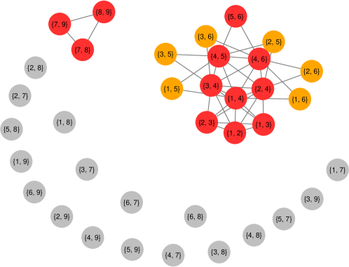
Figure 2: The conditional independence graph of Models 2 and 3 with population of nodes $\mathscr{N}\coloneqq\{1,\dots,9\}$, consisting of overlapping subpopulations $\mathscr{A}_{1}\coloneqq\{1,2,3,4\}$,  $\mathscr{A}_{2}\coloneqq\{4,5,6\}$,  and $\mathscr{A}_{3}\coloneqq\{7,8,9\}$. Edge variables $X_{i,j}$ are represented by circles with labels $\{i,j\}$. If nodes $i$ and $j$ share a subpopulation, $X_{i,j}$ is colored red. If nodes $i$ and $j$ do not share a subpopulation but belong to overlapping subpopulations, $X_{i,j}$ is colored orange. Otherwise, $X_{i,j}$ is colored gray.

To distinguish the random graph (representing data structure) from the conditional independence graph $\mathscr{G}$ (representing conditional independence structure, i.e., model structure), we call elements of $\mathscr{V}$ vertices rather than nodes, and elements of $\mathscr{E}$ edges rather than edge variables.

C.2.2 Conditional independence properties

We prove selected conditional independence properties that help establish consistency results and convergence rates for generalized $\beta$-models with dependent edges.

By Equations (2.1) and (2.2), for each $\{i,j\}\subset\mathscr{N}$,

$$\begin{array}[]{lllllllllllll}\varphi_{i,j}(x_{i,j},\,\bm{x}_{\mathscr{S}_{i,j}};\,{\rm Nature})\,\coloneqq\,a_{i,j}(x_{i,j})\,\exp\left((\theta_{i}+\theta_{j})\,x_{i,j}+\theta_{N+1}\,b_{i,j}(x_{i,j},\,\bm{x}_{\mathscr{S}_{i,j}})\right),\end{array}$$

where

$$\begin{array}[]{lllllllllllll}b_{i,j}(x_{i,j},\bm{x}_{\mathscr{S}_{i,j}})&\coloneqq&\begin{cases}0&\mbox{if }\mathscr{N}_{i}\cap\mathscr{N}_{j}=\emptyset\vspace{0.25cm}\\ x_{i,j}\,\mathbbm{1}\left(\displaystyle\sum\limits_{h\,\in\,\mathscr{N}_{i}\,\cap\,\mathscr{N}_{j}}x_{i,h}\,x_{j,h}\geq 1\right)&\mbox{if }\mathscr{N}_{i}\cap\mathscr{N}_{j}\neq\emptyset.\end{cases}\end{array}$$

Definition C.17.

Neighborhood intersection property. Consider a random graph model with a probability density function parameterized by (2.1) and (2.2). If $\mathscr{S}_{i,j}=\left\{\{a,b\}\subset\mathscr{N}\,:\,(a,b)\in\{i,j\}\times\{\mathscr{N}_{i}\,\cap\,\mathscr{N}_{j}\}\right\}$ for all pairs of nodes $\{i,j\}\subset\mathscr{N}$, then the random graph is said to satisfy the neighborhood intersection property.

By construction, generalized $\beta$-models with dependent edges satisfy the neighborhood intersection property, which implies conditional independence properties, including—but not limited to—the conditional independence properties established in Proposition C.18 below. Define

$$\begin{array}[]{lllllllllllll}\mathfrak{D}_{N}&\coloneqq&\big{\{}\{a,b\}\,:\,a\in\mathscr{N},\;b\in\mathscr{N}\setminus\{a\}\big{\}}.\end{array}$$

We will utilize $\mathfrak{D}_{N}$ as the index set of all possible edge variables, which will be useful in constructing statements which exclude certain edge variables.

Proposition C.18.

A random graph with overlapping subpopulations $\mathscr{A}_{k}$ of sizes $|\mathscr{A}_{k}|\geq 3$ ($k=1,\dots,K$) satisfying the neighborhood intersection property possesses the following conditional independence properties:

• For all pairs of nodes $\{i,j\}\subset\mathscr{N}$ such that $\mathscr{N}_{i}\,\cap\,\mathscr{N}_{j}=\emptyset$:

  $$\begin{array}[]{lllllllllllll}X_{i,j}&\mathchoice{\mathrel{\hbox to0.0pt{$\displaystyle\perp$\hss}\mkern 2.0mu{\displaystyle\perp}}}{\mathrel{\hbox to0.0pt{$\textstyle\perp$\hss}\mkern 2.0mu{\textstyle\perp}}}{\mathrel{\hbox to0.0pt{$\scriptstyle\perp$\hss}\mkern 2.0mu{\scriptstyle\perp}}}{\mathrel{\hbox to0.0pt{$\scriptscriptstyle\perp$\hss}\mkern 2.0mu{\scriptscriptstyle\perp}}}&\bm{X}_{\mathfrak{D}_{N}\setminus\,\{i,j\}}.\end{array}$$

• For all pairs of nodes $\{i,j\}\subset\mathscr{N}$ such that $\mathscr{N}_{i}\,\cap\,\mathscr{N}_{j}\neq\emptyset$ and there exists $k\in\{1,\ldots,K\}$ such that $\{i,j\}\subset\mathscr{A}_{k}$:

  $$\begin{array}[]{lllllllllllll}X_{i,j}&\mathchoice{\mathrel{\hbox to0.0pt{$\displaystyle\perp$\hss}\mkern 2.0mu{\displaystyle\perp}}}{\mathrel{\hbox to0.0pt{$\textstyle\perp$\hss}\mkern 2.0mu{\textstyle\perp}}}{\mathrel{\hbox to0.0pt{$\scriptstyle\perp$\hss}\mkern 2.0mu{\scriptstyle\perp}}}{\mathrel{\hbox to0.0pt{$\scriptscriptstyle\perp$\hss}\mkern 2.0mu{\scriptscriptstyle\perp}}}&\bm{X}_{\mathfrak{D}_{N}\setminus\,(\{i,j\}\,\cup\,\mathfrak{N}_{i,j})}\mid\bm{X}_{\mathfrak{N}_{i,j}},\end{array}$$

  where $\mathfrak{N}_{i,j}=\mathcal{J}_{i}^{(j)}\cup\mathcal{J}_{j}^{(i)}$, using the definition

  $$\begin{array}[]{lllllllllllll}\mathcal{J}_{t}^{(v)}&\coloneqq&\left[\bigcup\limits_{b\in\mathscr{N}_{t}\setminus\{v\}}\,\{v,b\}\right]\;\cup\;\left[\bigcup\limits_{b\in\mathscr{N}_{t}}\,\big{\{}\{a,b\}:(a,b)\in\{v,b\}\times\mathscr{N}_{v}\cap\mathscr{N}_{b}\big{\}}\right],\end{array}$$

  and with the property that

  $$\begin{array}[]{lllllllllllll}\mathfrak{N}_{i,j}&\subseteq&\big{\{}\{a,b\}\,:\,a\in\mathscr{N}_{i}\cup\mathscr{N}_{j},\,b\in\mathscr{N}_{i}\cup\mathscr{N}_{j}\setminus\{a\}\big{\}}.\end{array}$$

• For all pairs of nodes $\{i,j\}\subset\mathscr{N}$ such that $\mathscr{N}_{i}\,\cap\,\mathscr{N}_{j}\neq\emptyset$ and there exists no $k\in\{1,\ldots,K\}$ such that $\{i,j\}\subset\mathscr{A}_{k}$:

  $$\begin{array}[]{lllllllllllll}X_{i,j}&\mathchoice{\mathrel{\hbox to0.0pt{$\displaystyle\perp$\hss}\mkern 2.0mu{\displaystyle\perp}}}{\mathrel{\hbox to0.0pt{$\textstyle\perp$\hss}\mkern 2.0mu{\textstyle\perp}}}{\mathrel{\hbox to0.0pt{$\scriptstyle\perp$\hss}\mkern 2.0mu{\scriptstyle\perp}}}{\mathrel{\hbox to0.0pt{$\scriptscriptstyle\perp$\hss}\mkern 2.0mu{\scriptscriptstyle\perp}}}&\bm{X}_{\mathfrak{D}_{N}\setminus\,(\{i,j\}\,\cup\,\mathscr{S}_{i,j})}\mid\bm{X}_{\mathscr{S}_{i,j}}.\end{array}$$

  where $\mathscr{S}_{i,j}=\left\{\{a,b\}\subset\mathscr{N}\,:\,(a,b)\in\{i,j\}\times\{\mathscr{N}_{i}\,\cap\,\mathscr{N}_{j}\}\right\}$.

Proof of Proposition C.18. In the following, we use the characterizations of conditional independence due to Dawid [14], which relate factorization properties of probability density functions to conditional independence properties. Using these characterizations of conditional independence, we establish the conditional independence properties of Proposition C.18 by showing that, for each pair of nodes $\{i,j\}\subset\mathscr{N}$, there exists a subset of edge indices $\mathfrak{N}_{i,j}\subseteq\mathfrak{D}_{N}\setminus\{i,j\}$ and non-negative functions $g$ and $h$ such that the probability density function can be written as

$$\begin{array}[]{lllllllllllll}f_{{\rm Nature}}(\bm{x})&\propto&g(x_{i,j},\,\bm{x}_{\mathfrak{N}_{i,j}})\;h(\bm{x}_{\mathfrak{D}_{N}\setminus\{i,j\}}),\end{array}$$

where $\mathfrak{D}_{N}\coloneqq\{\{a,b\}\,:\,a\in\mathscr{N},\,b\in\mathscr{N}\setminus\{a\}\}$, implying that

$$\begin{array}[]{lllllllllllll}X_{i,j}&\mathchoice{\mathrel{\hbox to0.0pt{$\displaystyle\perp$\hss}\mkern 2.0mu{\displaystyle\perp}}}{\mathrel{\hbox to0.0pt{$\textstyle\perp$\hss}\mkern 2.0mu{\textstyle\perp}}}{\mathrel{\hbox to0.0pt{$\scriptstyle\perp$\hss}\mkern 2.0mu{\scriptstyle\perp}}}{\mathrel{\hbox to0.0pt{$\scriptscriptstyle\perp$\hss}\mkern 2.0mu{\scriptscriptstyle\perp}}}&\bm{X}_{\mathfrak{D}_{N}\setminus(\{i,j\}\,\cup\;\mathfrak{N}_{i,j})}\mid\bm{X}_{\mathfrak{N}_{i,j}}.\end{array}$$

Proposition C.18 assumes that the neighborhood intersection property is satisfied, allowing us to write

$$\begin{array}[]{lllllllllllll}f_{{\rm Nature}}(\bm{x})&\propto&\displaystyle\prod\limits_{i\,<\,j}^{N}\,\varphi_{i,j}(x_{i,j},\,\bm{x}_{\mathscr{S}_{i,j}}),\end{array}$$

where

$$\begin{array}[]{lllllllllllll}\mathscr{S}_{i,j}&=&\left\{\{v,w\}:(v,w)\in\{i,j\}\times\mathscr{N}_{i}\cap\mathscr{N}_{j}\right\},\end{array}$$

recalling the definition of the node neighborhood sets $\mathscr{N}_{i}$ ($i\in\mathscr{N}$):

$$\begin{array}[]{lllllllllllll}\mathscr{N}_{i}&=&\{h\in\mathscr{N}\setminus\{i\}\,:\,\mbox{ exists }k\in\{1,\ldots,K\}\mbox{ such that }\{i,h\}\subset\mathscr{A}_{k}\}.\end{array}$$

Condition 1: Consider any pair of nodes $\{i,j\}\subset\mathscr{N}$ with $\mathscr{N}_{i}\,\cap\,\mathscr{N}_{j}=\emptyset$, that is, nodes $i$ and $j$ neither belong to a common subpopulations nor belong to distinct subpopulations that overlap. Since $\{i,j\}\times\mathscr{N}_{i}\cap\mathscr{N}_{j}=\emptyset$,

$$\begin{array}[]{lllllllllllll}\varphi_{i,j}(x_{i,j},\,\bm{x}_{\mathscr{S}_{i,j}})&\equiv&\varphi_{i,j}(x_{i,j}).\end{array}$$

It remains to check whether any $\varphi_{a,b}$ with $\{a,b\}\neq\{i,j\}$ can be a function of $x_{i,j}$, which can happen in one of two different ways:

• $i\in\{a,b\}$ and $j\in\mathscr{N}_{a}\cap\mathscr{N}_{b}$, in which case, by the definition of the node neighborhood sets $\mathscr{N}_{v}$ ($v\in\mathscr{N}$), it must be that $j\in\mathscr{N}_{i}$; or

• $j\in\{a,b\}$ and $i\in\mathscr{N}_{a}\cap\mathscr{N}_{b}$, in which case, similarly, $i\in\mathscr{N}_{j}$.

We prove that there exists no $\varphi_{a,b}$ with $\{a,b\}\neq\{i,j\}$ which is a function of $x_{i,j}$ by contradiction. Note $i\in\mathscr{N}_{j}$ implies the existence of a $k\in\{1,\ldots,K\}$ such that $\{i,j\}\subset\mathscr{A}_{k}$. By assumption, $|\mathscr{A}_{k}|\geq 3$ for all $k\in\{1,\ldots,K\}$, implying there exists at least one other node $h\in\mathscr{A}_{k}\setminus\{i,j\}$. Thus, if $\{i,j,h\}\subseteq\mathscr{A}_{k}$, then both $h\in\mathscr{N}_{i}$ and $h\in\mathscr{N}_{j}$ must hold, violating the assumption that $\mathscr{N}_{i}\cap\mathscr{N}_{j}=\emptyset$. The case when $j\in\{a,b\}$ and $i\in\mathscr{N}_{a}\cap\mathscr{N}_{b}$ is proved similarly. Therefore, there cannot exist a pair of nodes $\{a,b\}\neq\{i,j\}$ such that $\varphi_{a,b}$ is a function of $x_{i,j}$. As a consequence, taking

$$\begin{array}[]{lllllllllllll}g(x_{i,j})&=&\varphi_{i,j}(x_{i,j})\end{array}$$

and

$$\begin{array}[]{lllllllllllll}h(\bm{x}_{\mathfrak{D}_{N}\setminus\{i,j\}})&=&\displaystyle\prod\limits_{a<b:\;\{a,b\}\,\neq\,\{i,j\}}^{N}\,\varphi_{a,b}(x_{a,b},\,\bm{x}_{\mathscr{S}_{a,b}})\end{array}$$

shows that $f_{{\rm Nature}}(\bm{x})$ can be written as

$$\begin{array}[]{lllllllllllll}f_{{\rm Nature}}(\bm{x})&\propto&g(x_{i,j})\;h(\bm{x}_{\mathfrak{D}_{N}\setminus\{i,j\}}),\end{array}$$

which implies $X_{i,j}\mathchoice{\mathrel{\hbox to0.0pt{$\displaystyle\perp$\hss}\mkern 2.0mu{\displaystyle\perp}}}{\mathrel{\hbox to0.0pt{$\textstyle\perp$\hss}\mkern 2.0mu{\textstyle\perp}}}{\mathrel{\hbox to0.0pt{$\scriptstyle\perp$\hss}\mkern 2.0mu{\scriptstyle\perp}}}{\mathrel{\hbox to0.0pt{$\scriptscriptstyle\perp$\hss}\mkern 2.0mu{\scriptscriptstyle\perp}}}\bm{X}_{\mathfrak{D}_{N}\setminus\{i,j\}}$, i.e., $X_{i,j}$ is independent of all others edges.

Condition 2: Consider any pair of nodes $\{i,j\}\subset\mathscr{N}$ with $\mathscr{N}_{i}\cap\mathscr{N}_{j}\neq\emptyset$ and such that there exists a $k\in\{1,\ldots,K\}$ such that $\{i,j\}\subset\mathscr{A}_{k}$. By definition, $\varphi_{i,j}(x_{i,j},\bm{x}_{\mathscr{S}_{i,j}})$ is a function of $x_{i,j}$. Recall the key condition for the neighborhood intersection assumption, which was that $\mathscr{S}_{a,b}$ satisfies

$$\begin{array}[]{lllllllllllll}\mathscr{S}_{a,b}&=&\left\{\{v,w\}:(v,w)\in\{a,b\}\times\mathscr{N}_{a}\,\cap\,\mathscr{N}_{b}\right\},&&\{a,b\}\subset\mathscr{N}.\end{array}$$

For any $\varphi_{a,b}(x_{a,b},\bm{x}_{\mathscr{S}_{a,b}})$ with $\{a,b\}\neq\{i,j\}$ to be a function of $x_{i,j}$, one of the following must hold:

1. $i\in\{a,b\}$ and $j\in\mathscr{N}_{a}\cap\mathscr{N}_{b}$, in which case, by the definition of the node neighborhood sets $\mathscr{N}_{v}$ ($v\in\mathscr{N}$), $j\in\mathscr{N}_{i}$; or

2. $j\in\{a,b\}$ and $i\in\mathscr{N}_{a}\cap\mathscr{N}_{b}$, in which case, similarly, $i\in\mathscr{N}_{j}$.

Consider the first case: $i\in\{a,b\}$ and $j\in\mathscr{N}_{a}\cap\mathscr{N}_{b}$, and without loss, take $a=i$. The condition for this case implies that $j\in\mathscr{N}_{i}\cap\mathscr{N}_{b}$. By assumption, $\{i,j\}\subset\mathscr{A}_{k}$ for some $k\in\{1,\ldots,K\}$, which implies $j\in\mathscr{N}_{i}$. If $j\in\mathscr{N}_{b}$, then $b\in\mathscr{N}_{j}$, implying $\varphi_{i,b}$ is a function of $x_{i,j}$ for all $\{i,b\}\subset\mathscr{N}$ with $b\in\mathscr{N}_{j}$. Applying the same argument to the second case where $j\in\{a,b\}$ and $i\in\mathscr{N}_{a}\cap\mathscr{N}_{b}$ reveals that $\varphi_{j,b}$ is a function of $x_{i,j}$ for all $\{j,b\}$ with $b\in\mathscr{N}_{i}$.

Summarily, $\varphi_{a,b}$ is a function of $x_{i,j}$ if it is in the following list:

• $\varphi_{i,j}(x_{i,j},\bm{x}_{\mathscr{S}_{i,j}})$, where $\{v,w\}\in\mathscr{S}_{i,j}$ if $(v,w)\in\{i,j\}\times\mathscr{N}_{i}\,\cap\,\mathscr{N}_{j}$.

• $\varphi_{i,b}(x_{i,b},\bm{x}_{\mathscr{S}_{i,b}})$ ($b\in\mathscr{N}_{j}$), where $\{v,w\}\in\mathscr{S}_{i,b}$ if $(v,w)\in\{i,b\}\times\mathscr{N}_{i}\,\cap\,\mathscr{N}_{b}$.

• $\varphi_{j,b}(x_{j,b},\bm{x}_{\mathscr{S}_{j,b}})$ ($b\in\mathscr{N}_{i}$), where $\{v,w\}\in\mathscr{S}_{j,b}$ if $(v,w)\in\{j,b\}\times\mathscr{N}_{j}\,\cap\,\mathscr{N}_{b}$.

This collection of functions is a function of all edge variables $X_{a,b}$ with indices $\{a,b\}$ in $\mathcal{J}_{i}^{(j)}\cup\mathcal{J}_{j}^{(i)}\cup\{i,j\}$, where

$$\begin{array}[]{lllllllllllll}\mathcal{J}_{t}^{(v)}&\coloneqq&\left[\bigcup\limits_{b\in\mathscr{N}_{t}\setminus\{v\}}\,\{v,b\}\right]\;\cup\;\left[\bigcup\limits_{b\in\mathscr{N}_{t}}\,\big{\{}\{a,b\}:(a,b)\in\{v,b\}\times\mathscr{N}_{v}\cap\mathscr{N}_{b}\big{\}}\right].\end{array}$$

Thus, there exist non-negative functions $g$ and $h$ such that the probability density function can be written as follows:

$$\begin{array}[]{lllllllllllll}f_{{\rm Nature}}(\bm{x})&\propto&g(x_{i,j},\bm{x}_{\mathfrak{N}_{i,j}})\;h(\bm{x}_{\mathfrak{D}_{N}\setminus\{i,j\}}),\end{array}$$

where $\mathfrak{N}_{i,j}=\mathcal{J}_{i}^{(j)}\cup\mathcal{J}_{j}^{(i)}$, implying that

$$\begin{array}[]{lllllllllllll}X_{i,j}&\mathchoice{\mathrel{\hbox to0.0pt{$\displaystyle\perp$\hss}\mkern 2.0mu{\displaystyle\perp}}}{\mathrel{\hbox to0.0pt{$\textstyle\perp$\hss}\mkern 2.0mu{\textstyle\perp}}}{\mathrel{\hbox to0.0pt{$\scriptstyle\perp$\hss}\mkern 2.0mu{\scriptstyle\perp}}}{\mathrel{\hbox to0.0pt{$\scriptscriptstyle\perp$\hss}\mkern 2.0mu{\scriptscriptstyle\perp}}}&\bm{X}_{\mathfrak{D}_{N}\setminus(\{i,j\}\,\cup\,\mathfrak{N}_{i,j})}\mid\bm{X}_{\mathfrak{N}_{i,j}}.\end{array}$$

As $\{i,j\}\subset\mathscr{N}_{i}\cup\mathscr{N}_{j}$,

$$\begin{array}[]{lllllllllllll}\mathfrak{N}_{i,j}&\subseteq&\big{\{}\{a,b\}\,:\,a\in\mathscr{N}_{i}\cup\mathscr{N}_{j},\,b\in\mathscr{N}_{i}\cup\mathscr{N}_{j}\setminus\{a\}\big{\}}.\end{array}$$

Condition 3: Consider any pair of nodes $\{i,j\}\subset\mathscr{N}$ with $\mathscr{N}_{i}\cap\mathscr{N}_{j}\neq\emptyset$ and such that there exists no $k\in\{1,\ldots,K\}$ such that $\{i,j\}\subset\mathscr{A}_{k}$. It is clear that $\varphi_{i,j}$ is a function of $x_{i,j}$. For any $\varphi_{a,b}(x_{a,b},\bm{x}_{\mathscr{S}_{a,b}})$ with $\{a,b\}\neq\{i,j\}$ to be a function of $x_{i,j}$, one of the following must hold:

• $i\in\{a,b\}$ and $j\in\mathscr{N}_{a}\cap\mathscr{N}_{b}$, in which case, by the definition of the node neighborhood sets $\mathscr{N}_{v}$ ($v\in\mathscr{N}$), it must be that $j\in\mathscr{N}_{i}$; or

• $j\in\{a,b\}$ and $i\in\mathscr{N}_{a}\cap\mathscr{N}_{b}$, in which case, similarly, $i\in\mathscr{N}_{j}$.

In both conditions, $i\in\mathscr{N}_{j}$ and $j\in\mathscr{N}_{i}$, which implies that $\{i,j\}\subset\mathscr{A}_{k}$ for some $k\in\{1,\ldots,K\}$, violating the assumption that no such $k$ exists. Thus, $\varphi_{a,b}(x_{a,b},\bm{x}_{\mathscr{S}_{a,b}})$ is a function of $x_{i,j}$ if and only if $\{a,b\}=\{i,j\}$. As a result, there exist non-negative functions $g$ and $h$ such that

$$\begin{array}[]{lllllllllllll}f_{{\rm Nature}}(\bm{x})&\propto&g(x_{i,j},\,\bm{x}_{\mathscr{S}_{i,j}})\;h(\bm{x}_{\mathfrak{D}_{N}\setminus\{i,j\}})\end{array}$$

which implies $X_{i,j}\,\mathchoice{\mathrel{\hbox to0.0pt{$\displaystyle\perp$\hss}\mkern 2.0mu{\displaystyle\perp}}}{\mathrel{\hbox to0.0pt{$\textstyle\perp$\hss}\mkern 2.0mu{\textstyle\perp}}}{\mathrel{\hbox to0.0pt{$\scriptstyle\perp$\hss}\mkern 2.0mu{\scriptstyle\perp}}}{\mathrel{\hbox to0.0pt{$\scriptscriptstyle\perp$\hss}\mkern 2.0mu{\scriptscriptstyle\perp}}}\,\bm{X}_{\mathfrak{D}_{N}\setminus(\{i,j\}\,\cup\,\mathscr{S}_{i,j})}\mid\bm{X}_{\mathscr{S}_{i,j}}$. ∎

Lemma C.19.

Consider Models 2 and 3. Then $\max_{t\in\mathscr{N}}\,|\mathscr{N}_{t}|\leq D_{N}$ and

$$\begin{array}[]{lllllllllllll}\max\limits_{t\in\mathscr{N}}\,\left|\left\{a\in\mathscr{N}\setminus\{t\}\,:\,\mathscr{N}_{a}\cap\mathscr{N}_{t}\neq\emptyset\right\}\right|&\leq&D_{N}^{2},\end{array}$$

where $D_{N}\coloneqq\max_{\{i,j\}\subset\mathscr{N}}\,|\mathfrak{N}_{i,j}|$.

Proof of Lemma C.19. By Proposition C.18, for any $\{i,j\}\subset\mathscr{N}$ satisfying $\mathscr{N}_{i}\,\cap\,\mathscr{N}_{j}\neq\emptyset$ and for which there exists $k\in\{1,\ldots,K\}$ such that $\{i,j\}\subset\mathscr{A}_{k}$, we have $\mathfrak{N}_{i,j}=\mathcal{J}_{i}^{(j)}\cup\mathcal{J}_{j}^{(i)}$, where, for all $\{t,v\}\subset\mathscr{N}$,

$$\begin{array}[]{lllllllllllll}\mathcal{J}_{t}^{(v)}&\coloneqq&\left[\bigcup\limits_{b\in\mathscr{N}_{t}\setminus\{v\}}\,\{v,b\}\right]\;\cup\;\left[\bigcup\limits_{b\in\mathscr{N}_{t}}\,\big{\{}\{a,b\}:(a,b)\in\{v,b\}\times\mathscr{N}_{v}\cap\mathscr{N}_{b}\big{\}}\right].\end{array}$$

Then, for each $t\in\mathscr{N}$, there exists $v\in\mathscr{N}\setminus\{t\}$ and $k\in\{1,\ldots,K\}$ such that $\{t,v\}\subset\mathscr{A}_{k}$, due to the assumption that $|\mathscr{A}_{k}|\geq 3$ for all $k\in\{1,\ldots,K\}$ under Models 2 and 3, implying that

$$\begin{array}[]{lllllllllllll}|\mathfrak{N}_{v,t}|\,=\,|\mathcal{J}_{t}^{(v)}\cup\mathcal{J}_{v}^{(t)}|\,\geq\,\left|\left[\bigcup\limits_{b\in\mathscr{N}_{t}\setminus\{v\}}\,\{v,b\}\right]\cup\left[\bigcup\limits_{b\in\mathscr{N}_{v}\setminus\{t\}}\,\{t,b\}\right]\right|\,\geq\,|\mathscr{N}_{t}|.\end{array}$$

Thus $D_{N}\coloneqq\max_{\{i,j\}\subset\mathscr{N}}\,|\mathfrak{N}_{i,j}|\geq|\mathscr{N}_{t}|$ for all $t\in\mathscr{N}$. Next, for all $t\in\mathscr{N}$,

$$\begin{array}[]{lllllllllllll}\left|\left\{a\in\mathscr{N}\setminus\{t\}\,:\,\mathscr{N}_{a}\cap\mathscr{N}_{t}\neq\emptyset\right\}\right|\,\leq\,\left|\bigcup\limits_{r\in\mathscr{N}_{t}}\,\mathscr{N}_{r}\right|\,\leq\,|\mathscr{N}_{t}|\,\left(\max\limits_{r\in\mathscr{N}}|\mathscr{N}_{r}|\right)\,\leq\,D_{N}^{2},\end{array}$$

using the above-proven fact that $\max_{t\in\mathscr{N}}\,|\mathscr{N}_{t}|\leq D_{N}$. ∎

C.2.3 Bounding the spectral norm of the coupling matrix

We bound the spectral norm $|\!|\!|\mathscr{D}_{N}({\rm Nature}^{\star})|\!|\!|_{2}$ of the coupling matrix $\mathscr{D}_{N}({\rm Nature}^{\star})$. Throughout, we adopt the notation used in Section 3 of the manuscript and denote the number of edge variables by $M=\binom{N}{2}$ and edge variables by $X_{1},\dots,X_{M}$.

Lemma C.20.

Consider Models 2 and 3. Assume that Assumption A is satisfied and that the data-generating parameter vector ${\rm Nature}^{\star}\in\bm{\Theta}=\mathbb{R}^{p}$ satisfies

$$\begin{array}[]{lllllllllllllllll}|\!|{\rm Nature}^{\star}|\!|_{\infty}&\leq&\dfrac{L+\vartheta\,\log N}{14\,(3+D_{N})}-\epsilon^{\star},\end{array}$$ (C.11)

where $L\in[0,\,\infty)$, $\vartheta\in[0,\,\infty)$, and $\epsilon^{\star}\in(0,\,\infty)$ are constants, independent of $N$ and $p$, and $\epsilon^{\star}$ is the same as in the definition of $\widetilde{\Lambda}_{N}({\rm Nature}^{\star})$ and $\widetilde{\Phi}_{N}({\rm Nature}^{\star})$.

1. If the subpopulations do not intersect ($\omega_{1}=\omega_{2}=0$) and ${\rm Nature}^{\star}\in\mathbb{R}^{N+1}$ satisfies condition (C.11) with $\vartheta\in[0,\,1/2-\alpha)$, then

   $$\begin{array}[]{lllllllllllll}|\!|\!|\mathscr{D}_{N}({\rm Nature}^{\star})|\!|\!|_{2}&\leq&1+4\,D_{N}^{2}.\end{array}$$

2. If the subpopulations do intersect ($\omega_{1}>0$) and ${\rm Nature}^{\star}\in\mathbb{R}^{N+1}$ satisfies condition (C.11) with $\vartheta=0$, then there exists finite constants $C_{1}>0$ and $C_{2}>0$, independent of $N$ and $p$, such that

   $$\begin{array}[]{lllllllllllll}|\!|\!|\mathscr{D}_{N}({\rm Nature}^{\star})|\!|\!|_{2}&\leq&1+4\,D_{N}^{2}+\omega_{1}\,C_{1}\,\exp(C_{2}\,D_{N}^{3}).\end{array}$$

Condition (C.11) is identical to condition (3.15) on page 20 of the main manuscript.

Proof of Lemma C.20. We adapt the coupling approach of van den Berg and Maes [39, pp. 759–760] from the literature on Gibbs measures and Markov random fields to coupling conditional distributions of subgraphs of random graphs. Let $i\in\mathscr{V}$ be any vertex of the conditional independence graph $\mathscr{G}$, corresponding to edge variable $X_{i}$, and consider any $\bm{x}_{1:i-1}\in\{0,1\}^{i-1}$. Define

$$\begin{array}[]{lllllllllllll}\mathbb{P}_{i,\bm{x}_{1:i-1},0}(\bm{X}_{i+1:M}=\bm{a})&\coloneqq&\mathbb{P}(\bm{X}_{i+1:M}=\bm{a}\mid\bm{X}_{1:i-1}=\bm{x}_{1:i-1},X_{i}=0)\end{array}$$

and

$$\begin{array}[]{lllllllllllll}\mathbb{P}_{i,\bm{x}_{1:i-1},1}(\bm{X}_{i+1:M}=\bm{a})&\coloneqq&\mathbb{P}(\bm{X}_{i+1:M}=\bm{a}\mid\bm{X}_{1:i-1}=\bm{x}_{1:i-1},X_{i}=1),\end{array}$$

where $\bm{X}_{1:i-1}=(X_{1},\dots,X_{i-1})$, $\bm{X}_{i+1:M}=(X_{i+1},\dots,X_{M})$, and $\bm{a}\in\{0,1\}^{M-i}$.

We divide the proof into three parts:

• Coupling conditional distributions of subgraphs.

• Bounding the elements of the coupling matrix $\mathscr{D}_{N}({\rm Nature}^{\star})$.

• Bounding the spectral norm $|\!|\!|\mathscr{D}_{N}({\rm Nature}^{\star})|\!|\!|_{2}$ of the coupling matrix $\mathscr{D}_{N}({\rm Nature}^{\star})$.

I. Coupling conditional distributions of subgraphs. Given any vertex $i\in\mathscr{V}$ of the conditional independence graph $\mathscr{G}$ and any $\bm{x}_{1:i-1}\in\{0,1\}^{i-1}$, we construct a coupling $(\bm{X}^{\star},\bm{X}^{\star\star})$ of the conditional probability distributions $\mathbb{P}_{i,\bm{x}_{1:i-1},0}$ and $\mathbb{P}_{i,\bm{x}_{1:i-1},1}$. Some background on coupling can be found in Lindvall [27].

It will be convenient to assume that the coupling $(\bm{X}^{\star},\bm{X}^{\star\star})$ takes on values in the set $\{0,1\}^{M}\times\{0,1\}^{M}$ rather than the set $\{0,1\}^{M-i}\times\{0,1\}^{M-i}$, where we set $(\bm{X}_{1:i-1}^{\star},\,X_{i}^{\star})=(\bm{x}_{1:i-1},\,0)$ and $(\bm{X}_{1:i-1}^{\star\star},\,X_{i}^{\star\star})=(\bm{x}_{1:i-1},\,1)$ with probability $1$. As a consequence, the random vectors $\bm{X}^{\star}\in\{0,1\}^{M}$ and $\bm{X}^{\star\star}\in\{0,1\}^{M}$ have the same dimension as random vector $\bm{X}\in\{0,1\}^{M}$. We construct a coupling of the conditional probability distributions $\mathbb{P}_{i,\bm{x}_{1:i-1},0}$ and $\mathbb{P}_{i,\bm{x}_{1:i-1},1}$ as follows:

1. Initialize the subset of vertices $\mathfrak{V}=\{1,\ldots,i\}$.

2. Check whether there exists a vertex $j\in\mathscr{V}\,\setminus\,\mathfrak{V}$ connected to a vertex $v\in\mathfrak{V}$ in the conditional independence graph $\mathscr{G}$ such that the coupling disagrees at vertex $v\in\mathfrak{V}$, in the sense that $X^{\star}_{v}\neq X_{v}^{\star\star}$.

   1. If such a vertex $j$ exists, pick the smallest such vertex, and let $(X_{j}^{\star},\,X_{j}^{\star\star})$ be distributed according to an optimal coupling of $\mathbb{P}(X_{j}=\,\cdot\,\mid\bm{X}_{\mathfrak{V}}=\bm{x}^{\star}_{\mathfrak{V}})$ and $\mathbb{P}(X_{j}=\,\cdot\,\mid\bm{X}_{\mathfrak{V}}=\bm{x}^{\star\star}_{\mathfrak{V}})$.

   2. If no such vertex $j$ exists, select the smallest $j\in\mathscr{V}\,\setminus\,\mathfrak{V}$ and let $(X_{j}^{\star},\,X_{j}^{\star\star})$ be distributed according to an optimal coupling of $\mathbb{P}(X_{j}=\,\cdot\,\mid\bm{X}_{\mathfrak{V}}=\bm{x}^{\star}_{\mathfrak{V}})$ and $\mathbb{P}(X_{j}=\,\cdot\,\mid\bm{X}_{\mathfrak{V}}=\bm{x}^{\star\star}_{\mathfrak{V}})$. In this case, an optimal coupling will ensure $X_{j}^{\star}=X_{j}^{\star\star}$ with probability $1$, as conditional independence properties and the equality of edge variables in the conditioning statement in this case will imply

      $$\begin{array}[]{lllllllllllll}\mathbb{P}(X_{j}=a\mid\bm{X}_{\mathfrak{V}}=\bm{x}^{\star}_{\mathfrak{V}})&=&\mathbb{P}(X_{j}=a\mid\bm{X}_{\mathfrak{V}}=\bm{x}^{\star\star}_{\mathfrak{V}}),&a\in\{0,1\},\end{array}$$

      resulting in a total variation distance of $0$.

3. In both steps, an optimal coupling exists [27, Theorem 5.2, p. 19], but it may not be unique. Any optimal coupling will do.

4. Replace $\mathfrak{V}$ by $\mathfrak{V}\,\cup\{j\}$ and repeat Step 2 until $\mathscr{V}\setminus\mathfrak{V}=\emptyset$.

Denote the resulting coupling distribution by $\mathbb{Q}_{i,\bm{x}_{1:i-1}}$. Lemma C.23 verifies that the above algorithm constructs a valid coupling of the conditional distributions $\mathbb{P}_{i,\bm{x}_{1:i-1},0}$ and $\mathbb{P}_{i,\bm{x}_{1:i-1},1}$, in the sense that the marginal distributions of $\bm{X}^{\star}$ and $\bm{X}^{\star\star}$ are $\mathbb{P}_{i,\bm{x}_{1:i-1},0}$ and $\mathbb{P}_{i,\bm{x}_{1:i-1},1}$, respectively.

For any two distinct vertices $i\in\mathscr{V}$ and $j\in\{i+1,\dots,M\}$ of the conditional independence graph $\mathscr{G}$, define the event $i\centernot{\longleftrightarrow}j$ to be the event that there exists a path of disagreement between $i$ and $j$ in $\mathscr{G}$. A path of disagreement $i\centernot{\longleftrightarrow}j$ between vertices $X_{i}$ and $X_{j}$ is a sequence of two or more distinct vertices $(X_{i},\dots,X_{j})$ in the conditional independence graph $\mathscr{G}$ starting at vertex $X_{i}$ and ending at vertex $X_{j}$, such that

• each subsequent pair of vertices $(X_{v},X_{w})$ in the sequence is connected by an edge in the conditional independence graph $\mathscr{G}$, which indicates the absence of conditional independence of vertices $X_{v}$ and $X_{w}$;

• the coupling $(\bm{X}^{\star}_{i+1:M},\bm{X}^{\star\star}_{i+1:M})\in\{0,1\}^{M-i}\times\{0,1\}^{M-i}$ with joint probability mass function $\mathbb{Q}_{{\rm Nature}^{\star},i,\bm{x}_{1:i-1}}$ disagrees at each vertex $X_{v}$ in the sequence, in the sense that $X_{v}^{\star}\neq X_{v}^{\star\star}$.

Theorem 1 of van den Berg and Maes [39, p. 753] shows that

$$\begin{array}[]{lllllllllllllllll}\mathbb{Q}_{i,\bm{x}_{1:i-1}}(X_{j}^{\star}\neq X_{j}^{\star\star})&=&\mathbb{Q}_{i,\bm{x}_{1:i-1}}(i\centernot{\longleftrightarrow}j)&\leq&\mathbb{B}_{\bm{\pi}}(i\centernot{\longleftrightarrow}j),\end{array}$$ (C.12)

where $\mathbb{B}_{\bm{\pi}}$ is a Bernoulli product measure on $\{0,1\}^{M}$ with probability vector $\bm{\pi}\in[0,1]^{M}$. The coordinates $\pi_{v}$ of $\bm{\pi}$ are given by

$$\begin{array}[]{lllllllllllll}\pi_{v}&\coloneqq&\begin{cases}0&\mbox{ if }v\in\{1,\ldots,i-1\}\vspace{0.25cm}\\ 1&\mbox{ if }v=i\vspace{0.25cm}\\ \max\limits_{(\bm{x}_{-v},\,\bm{x}_{-v}^{\prime})\,\in\,\{0,1\}^{M-1}\times\{0,1\}^{M-1}}\,\pi_{v,\,\bm{x}_{-v},\,\bm{x}_{-v}^{\prime}}&\mbox{ if }v\in\{i+1,\ldots,M\},\end{cases}\end{array}$$

where

$$\begin{array}[]{lllllllllllll}\pi_{v,\,\bm{x}_{-v},\,\bm{x}_{-v}^{\prime}}&\coloneqq&|\!|\mathbb{P}(\,\cdot\mid\bm{X}_{-v}=\bm{x}_{-v})-\mathbb{P}(\,\cdot\mid\bm{X}_{-v}^{\prime}=\bm{x}_{-v}^{\prime})|\!|_{{\tiny\mbox{TV}}}.\end{array}$$

Observe that the total variation distance

$$\begin{array}[]{lllllllllllll}|\!|\mathbb{P}(\,\cdot\mid\bm{X}_{-v}=\bm{x}_{-v})-\mathbb{P}(\,\cdot\mid\bm{X}_{-v}^{\prime}=\bm{x}_{-v}^{\prime})|\!|_{{\tiny\mbox{TV}}}\end{array}$$

is equal to

$$\begin{array}[]{lllllllllllll}\sup\limits_{x_{v}\,\in\,\{0,\,1\}}\,\left|\mathbb{P}(X_{v}=x_{v}\mid\bm{X}_{-v}=\bm{x}_{-v})-\mathbb{P}(X_{v}=x_{v}\mid\bm{X}_{-v}^{\prime}=\bm{x}_{-v}^{\prime})\right|.\end{array}$$

The Bernoulli product measure $\mathbb{B}_{\bm{\pi}}$ assumes that independent Bernoulli experiments are carried out at vertices $v\in\{1,\dots,M\}$. The Bernoulli experiment at vertex $v\in\{i+1,\dots,M\}$ has two possible outcomes: Either vertex $v$ is open, in the sense that the event $\{X_{v}^{\star}\neq X_{v}^{\star\star}\}$ occurs and hence vertex $v$ allows a path of disagreement from $i$ to $j$ to pass through, or vertex $v$ is closed. A vertex $v$ is open with probability $\pi_{v}$, and closed with probability $1-\pi_{v}$. By construction, vertices $v\in\{1,\ldots,i-1\}$ are closed with probability $1$, and vertex $i$ is open with probability $1$.

The coupling argument of van den Berg and Maes [39] is useful, in that it translates the hard problem of bounding probabilities of events involving dependent random variables into the more convenient problem of bounding probabilities of events involving independent random variables. Indeed, we can bound the above-diagonal elements $\mathscr{D}_{i,j}({\rm Nature}^{\star})$ of $\mathscr{D}_{N}({\rm Nature}^{\star})$ by

$$\begin{array}[]{lllllllllllllllll}\mathscr{D}_{i,j}({\rm Nature}^{\star})\,\coloneqq\,\sup\limits_{\bm{x}_{1:i-1}\in\{0,1\}^{i-1}}\,\mathbb{Q}_{i,\bm{x}_{1:i-1}}(X_{j}^{\star}\neq X_{j}^{\star\star})\,\leq\,\mathbb{B}_{\bm{\pi}}(i\centernot{\longleftrightarrow}j).\end{array}$$ (C.13)

By the construction of $\mathscr{D}_{N}({\rm Nature}^{\star})$, the below-diagonal and diagonal elements of $\mathscr{D}_{N}({\rm Nature}^{\star})$ are $0$ and $1$, respectively. We define $\pi^{\star}\in(0,1)$ by

$$\begin{array}[]{lllllllllllll}\pi^{\star}&\coloneqq&\max\limits_{1\leq v\leq M}\,\pi_{v},\end{array}$$

and note that Lemma C.24, together with the assumption that ${\rm Nature}^{\star}\in\bm{\Theta}_{N}=\mathbb{R}^{p}$ satisfies (C.11), implies that

$$\begin{array}[]{lllllllllllll}\pi^{\star}&\leq&\dfrac{1}{1+\exp(-L-\vartheta\log N)}&<&1,\end{array}$$

where $L\in[0,\infty)$ and $\vartheta\in[0,\infty)$ are the same constants as in (C.11), assumed to be independent of $N$ and $p$. Let

$$\begin{array}[]{lllllllllllll}U&\coloneqq&\dfrac{1}{1+\exp(-L-\vartheta\log N)}\end{array}$$

and define the vector $\bm{\xi}\in[0,1]^{M}$ by

$$\begin{array}[]{lllllllllllll}\xi_{i}&\coloneqq&\begin{cases}0&\mbox{ if }v\in\{1,\ldots,i-1\}\vspace{0.25cm}\\ 1&\mbox{ if }v=i\vspace{0.25cm}\\ U&\mbox{ if }v\in\{i+1,\ldots,M\}\end{cases}.\end{array}$$

Observe that the probabilities $\mathbb{B}_{\bm{\pi}}(i\centernot{\longleftrightarrow}j)$ of the events $\{i\centernot{\longleftrightarrow}j\}$ are non-decreasing in the coordinates of $\bm{\pi}$, so that

$$\begin{array}[]{lllllllllllll}\mathbb{B}_{\bm{\pi}}(i\centernot{\longleftrightarrow}j)&\leq&\mathbb{B}_{\bm{\xi}}(i\centernot{\longleftrightarrow}j).\end{array}$$

We bound the elements $\mathscr{D}_{i,j}({\rm Nature}^{\star})$ of $\mathscr{D}_{N}({\rm Nature}^{\star})$ by bounding the probabilities $\mathbb{B}_{\bm{\xi}}(i\centernot{\longleftrightarrow}j)$ of the events $\{i\centernot{\longleftrightarrow}j\}$.

II. Bounding the elements of the coupling matrix $\mathscr{D}_{N}({\rm Nature}^{\star})$. To bound the elements $\mathscr{D}_{i,j}({\rm Nature}^{\star})$ of $\mathscr{D}_{N}({\rm Nature}^{\star})$, we bound the probabilities $\mathbb{B}_{\bm{\xi}}(i\centernot{\longleftrightarrow}j)$ of the events $\{i\centernot{\longleftrightarrow}j\}$ using Assumption A. To do so, define

$$\begin{array}[]{lllllllllllll}\mathscr{S}_{\mathscr{G},i,k}&\coloneqq&\left\{v\in\mathscr{V}\setminus\{i\}\,:\,d_{\mathscr{G}}(i,v)=k\right\},&&k=1,\ldots,M-1,\end{array}$$

where $d_{\mathscr{G}}(i,v)$ is the graph distance (i.e., the length of the shortest path) between vertices $i\in\mathscr{V}$ and $v\in\mathscr{V}$ in the conditional independence graph $\mathscr{G}$. The set $\mathscr{S}_{\mathscr{G},i,k}\subseteq\mathscr{V}$ represents the subset of vertices in the conditional independence graph $\mathscr{G}$ at graph distance $k$ from vertex $i$ in $\mathscr{G}$.

We bound $\mathbb{B}_{\bm{\xi}}(i\centernot{\longleftrightarrow}j)$ by placing restrictions on the subpopulation structure, which determines which edges are present in $\mathscr{G}$. To do so, define the subpopulation graph $\mathscr{G}_{\mathscr{A}}$ to be the graph with the set of subpopulations $\{\mathscr{A}_{1},\ldots,\mathscr{A}_{K}\}$ as vertices and edges between vertices $\mathscr{A}_{r}$ and $\mathscr{A}_{l}$ if and only if $\mathscr{A}_{r}\cap\mathscr{A}_{l}\neq\emptyset$. In $\mathscr{G}_{\mathscr{A}}$, two vertices corresponding to subpopulations $\mathscr{A}_{r}$ and $\mathscr{A}_{l}$ are connected by an edge if and only if they overlap. Let $d_{\mathscr{G}_{\mathscr{A}}}(\mathscr{A}_{r},\mathscr{A}_{l})$ denote the graph distance (i.e., the length of the shortest path) between vertices $\mathscr{A}_{r}$ and $\mathscr{A}_{l}$ in $\mathscr{G}_{\mathscr{A}}$. Define, for all $\mathscr{A}_{r}\in\{\mathscr{A}_{1},\ldots,\mathscr{A}_{K}\}$ and $k\in\{1,\ldots,K-1\}$,

$$\begin{array}[]{lllllllllllll}\mathscr{V}_{\mathscr{A}_{r},k}&\coloneqq&\big{\{}\mathscr{A}_{l}\in\{\mathscr{A}_{1},\ldots,\mathscr{A}_{K}\}\setminus\{\mathscr{A}_{r}\}\,:\,d_{\mathscr{G}_{\mathscr{A}}}(\mathscr{A}_{r},\,\mathscr{A}_{l})=k\big{\}}.\end{array}$$

Let $g:\{1,2,\ldots\}\mapsto[0,\,\infty)$ be such that, for all $K\in\{1,2,\ldots\}$,

$$\begin{array}[]{lllllllllllll}|\mathscr{V}_{\mathscr{A}_{r},k}|&\leq&g(k),&k\in\{1,\ldots,K-1\},&&\mbox{for all }\mathscr{A}_{r}\in\{\mathscr{A}_{1},\ldots,\mathscr{A}_{K}\}.\end{array}$$

In words, $g(k)$ bounds the number of subpopulations at graph distance $k$ from any given subpopulation in $\mathscr{G}_{\mathscr{A}}$ for all conceivable subpopulations and thus all conceivable subpopulation structures, i.e., for all $\mathscr{G}_{\mathscr{A}}$ defined for subpopulations $\mathscr{A}_{1},\ldots,\mathscr{A}_{K}$ at all values of $K\in\{1,2,\ldots\}$.

Models 2 and 3 satisfy Definition C.17 and posses the neighborhood intersection property. By Proposition C.18, the dependence neighborhood of any edge variable $X_{i}$ between nodes $\{a,b\}\subset\mathscr{N}$ is not larger than the subset of edge indices contained in the set $\mathscr{M}_{a,b}\coloneqq\big{\{}\{c,d\}\,:\,c\in\mathscr{N}_{a}\cup\mathscr{N}_{b},\,d\in\mathscr{N}_{a}\cup\mathscr{N}_{b}\setminus\{c\}\big{\}}$, i.e., the edge variables contained in the set $\mathfrak{N}_{i}$ will correspond to edge variables between pairs of nodes in $\mathscr{M}_{a,b}$. We construct a graph covering $\mathscr{G}^{\star}$ of the conditional independence graph $\mathscr{G}$ as follows:

1. Initialize $\mathscr{G}^{\star}$ with the same set of vertices and edges as $\mathscr{G}$.

2. For each vertex $X_{i}$ in $\mathscr{G}$ corresponding to an edge variable between nodes $\{a,b\}\subset\mathscr{N}$ with degree greater than $0$ in $\mathscr{G}$, add edges between $X_{i}$ and any other edge variables $X_{j}$ contained in the subgraph $\bm{X}_{\mathscr{M}_{a,b}}$ which are not already present in $\mathscr{G}$.

The construction of $\mathscr{G}^{\star}$ ensures that the dependence neighborhood of any given vertex $X_{i}$ in $\mathscr{G}^{\star}$ corresponding to the edge variable between pair of nodes $\{a,b\}\subset\mathscr{N}$ is either empty or is equal to the set of vertices corresponding to edge variables contained in the subgraph $\bm{X}_{\mathscr{M}_{a,b}}$. Moreover, the fact that $\mathscr{G}\subseteq\mathscr{G}^{\star}$ implies

$$\begin{array}[]{lllllllllllll}\mathbb{B}_{\bm{\xi}}(i\centernot{\longleftrightarrow}j\mbox{ in }\mathscr{G})&\leq&\mathbb{B}_{\bm{\xi}}(i\centernot{\longleftrightarrow}j\mbox{ in }\mathscr{G}^{\star}).\end{array}$$

In words, the probability of the existence of a path of disagreement does not decrease through the addition of edges in the graph. Henceforth and for ease of presentation, the event $i\centernot{\longleftrightarrow}j$ will represent a path of disagreement in the graph covering $\mathscr{G}^{\star}$ of $\mathscr{G}$ and we will assume $\mathscr{S}_{i,k}\equiv\mathscr{S}_{\mathscr{G}^{\star},i,k}$.

We bound each $|\mathscr{S}_{i,k}|$ ($k\in\{1,2,\ldots\}$) for arbitrary $i\in\mathscr{V}$ with non-zero degree in $\mathscr{G}^{\star}$:

• Bounding $|\mathscr{S}_{i,1}|$. Let $X_{i}$ denote the edge variable between pair of nodes $\{a,b\}\subset\mathscr{N}$. By definition, $\mathscr{S}_{i,1}$ contains all vertices in $\mathscr{G}^{\star}$ corresponding to edge variables $X_{j}$ which lie in the dependence neighborhood of edge variable $X_{i}$ in $\mathscr{G}^{\star}$. By the construction of $\mathscr{G}^{\star}$, the dependence neighborhood of edge variable $X_{i}$ in $\mathscr{G}^{\star}$ is equal to the set of edge variables contained in the subgraph $\bm{X}_{\mathscr{M}_{a,b}}$, the number of which is bounded above by $4\,D_{N}^{2}$:

  $$\begin{array}[]{lllllllllllll}|\mathscr{M}_{a,b}|\leq|\mathscr{N}_{a}\cup\mathscr{N}_{b}|^{2}\leq(|\mathscr{N}_{a}|+|\mathscr{N}_{b}|)^{2}\leq(2\,\max\{|\mathscr{N}_{a}|,\,|\mathscr{N}_{b}|\})^{2}\leq 4\,D_{N}^{2},\end{array}$$

  where by Lemma C.19, $D_{N}\geq\max_{t\in\mathscr{N}}\,|\mathscr{N}_{t}|$. Hence, $|\mathscr{S}_{i,1}|\leq 4\,D_{N}^{2}$.

• Bounding $|\mathscr{S}_{i,2}|$. Consider any $j\in\mathscr{S}_{i,2}$ and let $X_{i}$ denote the edge variable between pair of nodes $\{a,b\}\subset\mathscr{N}$. The shortest path between edge variables $X_{i}$ and $X_{j}$ in $\mathscr{G}^{\star}$ is of length $2$, implying the following:

  1. $X_{j}$ is not in the dependence neighborhood of $X_{i}$ in $\mathscr{G}^{\star}$.

  2. In $\mathscr{G}^{\star}$, there is at least one edge variable $X_{l}$ in the dependence neighborhood of $X_{i}$ such that $X_{j}$ is likewise in the dependence neighborhood of $X_{l}$.

  By the construction of $\mathscr{G}^{\star}$, facts (F.1) and (F.2) imply there exist

  • a pair of nodes $\{v,w\}\subseteq\mathscr{N}_{a}\cup\mathscr{N}_{b}$ such that $X_{l}$ is the edge variable between $\{v,w\}$, and

  • a pair of nodes $\{c,d\}\subseteq\mathscr{N}_{v}\cup\mathscr{N}_{w}$ such that $X_{j}$ is the edge variable between $\{c,d\}$ and $\{c,d\}\not\subseteq\mathscr{N}_{a}\cup\mathscr{N}_{b}$, otherwise $X_{j}$ would be in the dependence neighborhood of $X_{i}$, violating the assumption that $j\in\mathscr{S}_{i,2}$.

  Recall the definition, for all $v\in\mathscr{N}$,

  $$\begin{array}[]{lllllllllllll}\mathscr{N}_{v}&\coloneqq&\{w\in\mathscr{N}\setminus\{v\}\,:\,\mbox{exists }r\in\{1,\ldots,K\}\mbox{ such that }\{v,w\}\subset\mathscr{A}_{r}\}.\end{array}$$

  As $\{c,d\}\subseteq\mathscr{N}_{v}\cup\mathscr{N}_{w}$, there must exist $r,t\in\{1,\ldots,K\}$ such that:

  • either $\{c,v\}\subset\mathscr{A}_{r}$ or $\{c,w\}\subset\mathscr{A}_{r}$, and

  • either $\{d,v\}\subset\mathscr{A}_{t}$ or $\{d,w\}\subset\mathscr{A}_{t}$.

  Since $\{c,d\}\not\subseteq\mathscr{N}_{a}\cup\mathscr{N}_{b}$, therefore $\{a,b\}\not\subseteq\mathscr{A}_{r}\cup\mathscr{A}_{t}\subseteq\mathscr{N}_{c}\cup\mathscr{N}_{d}$. Finally, $\{v,w\}\subseteq\mathscr{N}_{a}\cup\mathscr{N}_{b}$ implies that there exists $n,m\in\{1,\ldots,K\}$ such that

  • either $\{v,a\}\subset\mathscr{A}_{n}$ or $\{v,b\}\subset\mathscr{A}_{n}$, and

  • either $\{w,a\}\subset\mathscr{A}_{m}$ or $\{w,b\}\subset\mathscr{A}_{m}$.

  As a result, $(\mathscr{A}_{n}\cup\mathscr{A}_{m})\,\cap\,(\mathscr{A}_{r}\cup\mathscr{A}_{t})\neq\emptyset$, implying either $v$ or $w$ belong to a subpopulation $\mathscr{A}_{z}\not\subseteq\mathscr{N}_{a}\cup\mathscr{N}_{b}$ ($z\in\{1,\ldots,K\}$) for which $d_{\mathscr{G}_{\mathscr{A}}}(\mathscr{A}_{z},\mathscr{A}_{y})=1$ for some $y\in\{1,\ldots,K\}$ with $\mathscr{A}_{y}\subseteq\mathscr{N}_{a}\cup\mathscr{N}_{b}$, i.e., a subpopulation with graph distance at least $1$ in $\mathscr{G}_{\mathscr{A}}$ from all subpopulations represented in $\mathscr{N}_{a}\cup\mathscr{N}_{b}$ and equal to $1$ for at least one such subpopulation. The same holds for either $c$ or $d$. Thus,

  $$\begin{array}[]{lllllllllllll}|\mathscr{S}_{i,2}|&\leq&2\,D_{N}^{3}\,(g(1)+1)\,g(1),\end{array}$$

  which follows from the following argument:

  • First, the number of subpopulations contained in $\mathscr{N}_{a}\cup\mathscr{N}_{b}$ is bounded above by $2(g(1)+1)$, because $g(1)$ bounds the number of subpopulations which overlap with any other subpopulation, so that $g(1)+1$ bounds the number of subpopulations to which any node $a\in\mathscr{N}$ or $b\in\mathscr{N}$ may belong;

  • Second, the number of subpopulations with graph distance $1$ in the subpopulation graph $\mathscr{G}_{\mathscr{A}}$ to any subpopulation represented in $\mathscr{N}_{a}\cup\mathscr{N}_{b}$ is bounded above by $2\,(g(1)+1)\,g(1)$;

  • Third, note that either $c$ or $d$ must be in one of the subpopulations with graph distance $1$ in $\mathscr{G}_{\mathscr{A}}$ to at least one of the subpopulations represented in $\mathscr{N}_{a}\cup\mathscr{N}_{b}$. Without loss, let this be $c$. Then the total number of such nodes $c$ which are contained in one of the aforementioned subpopulations at graph distance $1$ is bounded above by $2\,D_{N}\,(g(1)+1)\,g(1)$, using the bound $|\mathscr{A}_{k}|\leq|\mathscr{N}_{i}|\leq D_{N}$ from Lemma C.19 which holds for all $k\in\{1,\ldots,K\}$ and $i\in\mathscr{A}_{k}$.

  • Finally, we bound the number of possible $d$ that may be paired with $c$. Note $X_{j}$ has non-zero degree in $\mathscr{G}^{\star}$. By Proposition C.18, $X_{j}$ is independent of all other edges if $\mathscr{N}_{c}\cap\mathscr{N}_{d}=\emptyset$. Thus, we bound the number of edge variables $X_{j}$ between node $c\in\mathscr{N}$ and nodes $d\in\mathscr{N}\setminus\{c\}$ for which $\mathscr{N}_{c}\cap\mathscr{N}_{d}\neq\emptyset$ using Lemma C.19:

    $$\begin{array}[]{lllllllllllll}\left|\left\{d\in\mathscr{N}\setminus\{c\}\,:\,\mathscr{N}_{c}\cap\mathscr{N}_{d}\neq\emptyset\right\}\right|&\leq&D_{N}^{2}.\end{array}$$

    Hence, the number of such $d$ (for a given $c$) numbers no more than $D_{N}^{2}$, the total of which is bounded above by $2\,D_{N}^{3}\,(g(1)+1)\,g(1)$.

• Bounding $|\mathscr{S}_{i,k}|$ for $k\in\{3,4,\ldots\}$. Consider any $k\in\{3,4,\ldots\}$ and any $j\in\mathscr{S}_{i,k}$. Let $X_{i}$ be the edge variable between nodes $\{a,b\}\subset\mathscr{N}$ and $X_{j}$ be the edge variable between pair of nodes $\{c,d\}\subset\mathscr{N}$. For $j\in\mathscr{S}_{i,k}$, there must exist an $l\in\mathscr{S}_{i,k-1}$ such that $j\in\mathscr{S}_{l,1}$. Let $X_{l}$ be the edge variable between nodes $\{v,w\}\subset\mathscr{N}$. Leveraging arguments from the case bounding $|\mathscr{S}_{i,1}|$ above, $\{c,d\}\subseteq\mathscr{N}_{v}\cup\mathscr{N}_{w}$, implying both $c$ and $d$ belong to at least one subpopulation to which either $v$ or $w$ also belong. Assume the following:

  • $h\in\mathscr{S}_{i,k-1}$ if and only if $X_{h}$ is an edge variable between nodes $\{r,t\}\subset\mathscr{N}$ and either $r$ or $t$ belongs to a subpopulation at graph distance $k-2$ in $\mathscr{G}_{\mathscr{A}}$ to a subpopulation represented in $\mathscr{N}_{a}\cup\mathscr{N}_{b}$ and not less than $k-2$ to all others in $\mathscr{N}_{a}\cup\mathscr{N}_{b}$.

  • $h\in\mathscr{S}_{i,k-2}$ if and only if $X_{h}$ is an edge variable between nodes $\{r,t\}\subset\mathscr{N}$ and either $r$ or $t$ belongs to a subpopulation at graph distance $k-3$ in $\mathscr{G}_{\mathscr{A}}$ to a subpopulation represented in $\mathscr{N}_{a}\cup\mathscr{N}_{b}$ and not less than $k-3$ to all others in $\mathscr{N}_{a}\cup\mathscr{N}_{b}$.

  We have shown above that (A.1) and (A.2) are satisfied when $k=3$:

  • $h\in\mathscr{S}_{i,1}$ corresponds to edge variables $X_{h}$ between nodes $\{r,t\}\subset\mathscr{N}_{a}\cup\mathscr{N}_{b}$, in which case both $r$ and $t$ belong to a subpopulation represented in $\mathscr{N}_{a}\cup\mathscr{N}_{b}$ and therefore have graph distance $0$ in $\mathscr{G}_{\mathscr{A}}$ to a subpopulation represented in $\mathscr{N}_{a}\cup\mathscr{N}_{b}$.

  • $h\in\mathscr{S}_{i,2}$ corresponds to edge variables $X_{h}$ between nodes $\{r,t\}\subset\mathscr{N}$ for which either $r$ or $t$ belongs to a subpopulation which is not represented in $\mathscr{N}_{a}\cup\mathscr{N}_{b}$, but which is at graph distance $1$ in $\mathscr{G}_{\mathscr{A}}$ to a subpopulation represented in $\mathscr{N}_{a}\cup\mathscr{N}_{b}$, and at graph distance no less than $1$ to all others in $\mathscr{N}_{a}\cup\mathscr{N}_{b}$.

  Assumptions (A.1) and (A.2) require that neither $v$ nor $w$ belong to a subpopulation at graph distance less than or equal to $k-2$ in $\mathscr{G}_{\mathscr{A}}$ from any subpopulation represented in $\mathscr{N}_{a}\cup\mathscr{N}_{b}$. Leveraging the argument used in the case bounding $|\mathscr{S}_{i,2}|$: For $\{c,d\}\subseteq\mathscr{N}_{v}\cup\mathscr{N}_{w}$, either $c$ or $d$ must belong to a subpopulation $\mathscr{A}_{r}$ ($r\in\{1,\ldots,K\}$) jointly with either $v$ or $w$ which is at graph distance at least $k-1$ in in $\mathscr{G}_{\mathscr{A}}$ from any subpopulation represented in $\mathscr{N}_{i}\cup\mathscr{N}_{j}$. Thus, there must exist some $q\in\{1,\ldots,K\}$ such that $\mathscr{A}_{r}\cap\mathscr{A}_{q}\neq\emptyset$ and for which both of the following are satisfied:

  • $d_{\mathscr{G}_{\mathscr{A}}}(\mathscr{A}_{q},\mathscr{A}_{y})\geq k-2$ for all $y\in\{1,\ldots,K\}$ satisfying $\mathscr{A}_{y}\subseteq\mathscr{N}_{a}\cup\mathscr{N}_{b}$;

  • $d_{\mathscr{G}_{\mathscr{A}}}(\mathscr{A}_{q},\mathscr{A}_{y})=k-2$ for at least one $y\in\{1,\ldots,K\}$ satisfying $\mathscr{A}_{y}\subseteq\mathscr{N}_{a}\cup\mathscr{N}_{b}$.

  Hence, there exists at least one $y\in\{1,\ldots,K\}$ satisfying $\mathscr{A}_{y}\subseteq\mathscr{N}_{a}\cup\mathscr{N}_{b}$ for which $d_{\mathscr{G}_{\mathscr{A}}}(\mathscr{A}_{r},\mathscr{A}_{y})=k-1$. Repeating the counting argument from the case bounding $|\mathscr{S}_{i,2}|$ above shows that the number of such pairs $\{a,b\}\subset\mathscr{N}$ is bounded above by

  $$\begin{array}[]{lllllllllllll}|\mathscr{S}_{i,k}|&\leq&2\,D_{N}^{3}\,(g(1)+1)\,g(k-1),\end{array}$$

  and the result is proved by induction.

From the above, we have the bounds $|\mathscr{S}_{i,1}|\leq 4\,D_{N}^{2}$ and

$$\begin{array}[]{lllllllllllllllll}|\mathscr{S}_{i,k}|&\leq&2\,D_{N}^{3}\,(g(1)+1)\,g(k-1),&&k\in\{2,3,\ldots\}.\end{array}$$ (C.14)

We proceed with bounding $\mathscr{D}_{i,j}({\rm Nature}^{\star})$ under Assumption A. Define the function $g:\{1,2,\ldots\}\mapsto[0,\infty)$ by

$$\begin{array}[]{lllllllllllllllll}g(k)&=&\omega_{1}+\dfrac{\omega_{2}}{2\,D^{3}_{N}}\,\log\,k,&&k\in\{1,2,\dots\},\end{array}$$ (C.15)

where $\omega_{1}\geq 0$ and $\omega_{2}\in[0,\omega_{1}]$ are independent of $N$ and $p$ by Assumption A, and $\omega_{2}\in[0,\omega_{1}]$ additionally satisfies

$$\begin{array}[]{lllllllllllll}\omega_{2}&<&\dfrac{1}{(\omega_{1}+1)\,|\log(1-U)|}.\end{array}$$

Using (C.15) and (C.14), we obtain the bounds $|\mathscr{S}_{i,1}|\leq 4\,D_{N}^{2}$ and

$$\begin{array}[]{lllllllllllll}|\mathscr{S}_{i,k}|&\leq&(\omega_{1}+1)\,(2\,D_{N}^{3}\,\omega_{1}+\omega_{2}\,\log(k-1)),&&k\in\{2,3,\ldots\}.\end{array}$$

By construction,

$$\begin{array}[]{lllllllllllll}\mathbb{B}_{\bm{\xi}}(v\mbox{ is open in }\mathscr{G}^{\star})&\leq&U&<&1,&&v\in\{i+1,\ldots,M\}.\end{array}$$

For there to be a path of disagreement $i\centernot{\longleftrightarrow}j$ in $\mathscr{G}^{\star}$ between a vertex $i\in\{1,\ldots,M\}$ and $j\in\mathscr{S}_{i,k}$, there must be at least one open vertex in each of the sets $\mathscr{S}_{i,1},\ldots,\mathscr{S}_{i,k-1}$ and $j$ must be open (placing no restrictions on the connectedness of vertices within sets or between two sequential sets); note that $i$ is open with probability $1$. The probability that there exists at least one open vertex $v\in\mathscr{S}_{i,1}$ is bounded above by

$$\begin{array}[]{lllllllllllll}1-(1-U)^{|\mathscr{S}_{i,1}|}&\leq&1-(1-U)^{4\,D_{N}^{2}}&\leq&1,\end{array}$$

and for $k\in\{2,3,\ldots\}$, the same is bounded above by

$$\begin{array}[]{lllllllllllll}1-(1-U)^{|\mathscr{S}_{i,k}|}&\leq&1-(1-U)^{(\omega_{1}+1)\,(2\,D_{N}^{3}\,\omega_{1}+\omega_{2}\,\log(k-1))}\vspace{0.25cm}\\ &=&1-(1-U)^{C_{1}D_{N}^{3}+C_{2}\log(k-1)},\end{array}$$

defining $C_{1}\coloneqq 2\,\omega_{1}\,(\omega_{1}+1)\in[0,\infty)$ and $C_{2}\coloneqq\omega_{2}\,(\omega_{1}+1)\in[0,\infty)$. Since the events that vertices are open are independent under the Bernoulli product measure $\mathbb{B}_{\bm{\xi}}$, we obtain

$$\begin{array}[]{lllllllllllll}\mathbb{B}_{\bm{\xi}}(i\centernot{\longleftrightarrow}j)&\leq&U\,\left[1-(1-U)^{4D_{N}^{2}}\right]\displaystyle\prod\limits\limits_{l=2}^{k-1}\,\left[1-(1-U)^{C_{1}D_{N}^{3}+C_{2}\log(l-1)}\right]\vspace{0.25cm}\\ &\leq&U\,\left[1-(1-U)^{4D_{N}^{2}}\right]\,\left[1-(1-U)^{C_{1}D_{N}^{3}+C_{2}\log(k-2)}\right]^{k-2}\vspace{0.25cm}\\ &\leq&\left[1-(1-U)^{C_{1}D_{N}^{3}+C_{2}\log(k-2)}\right]^{k-2},\end{array}$$

by the monotonicity of logarithms. We then bound

$$\begin{array}[]{lllllllllllll}1-(1-U)^{C_{1}D_{N}^{3}+C_{2}\log(k-2)}&\leq&\exp\left(-(1-U)^{C_{1}D_{N}^{3}+C_{2}\log(k-2)}\right),\end{array}$$

using the inequality $1-z\leq\exp(-z)$ ($z\in(0,1)$). We proceed by writing

$$\begin{array}[]{lllllllllllll}&&\exp\left(-(1-U)^{C_{1}D_{N}^{3}+C_{2}\log(k-2)}\right)\vspace{0.25cm}\vspace{0.25cm}\\ &=&\exp\left(-\exp\left(\left[C_{1}\,D_{N}^{3}+C_{2}\log(k-2)\right]\,\log(1-U)\right)\right)\vspace{0.25cm}\vspace{0.25cm}\\ &=&\exp\left(-\exp\left(-\left[C_{1}\,D_{N}^{3}+C_{2}\log(k-2)\right]\,|\log(1-U)|\right)\right)\vspace{0.25cm}\vspace{0.25cm}\\ &=&\exp\left(-\exp(-C_{1}\,D_{N}^{3}\,|\log(1-U)|)\;(k-2)^{-C_{2}\,|\log(1-U)|}\right),\end{array}$$

where in the above we used the fact that $\log(1-U)<0$. Define

$$\begin{array}[]{lllllllllllll}A&\coloneqq&\exp(-C_{1}\,D_{N}^{3}\,|\log(1-U)|)&\in&(0,1),\end{array}$$

noting that $D_{N}\geq 1$ under Models 2 and 3. Then

$$\begin{array}[]{lllllllllllll}\left[1-(1-U)^{C_{1}D_{N}^{3}+C_{2}\log(k-2)}\right]^{k-2}&\leq&\left[\exp\left(-A\,(k-2)^{-C_{2}\,|\log(1-U)|}\right)\right]^{k-2}\vspace{0.25cm}\vspace{0.25cm}\\ &=&\exp\left(-A\,(k-2)^{1-C_{2}\,|\log(1-U)|}\right),\end{array}$$

demonstrating the bound (for $i\in\{1,\ldots,M\}$ and $j\in\mathscr{S}_{i,k}$)

$$\begin{array}[]{lllllllllllll}\mathbb{B}_{\bm{\pi}}(i\centernot{\longleftrightarrow}j)&\leq&\mathbb{B}_{\bm{\xi}}(i\centernot{\longleftrightarrow}j)&\leq&\exp\left(-A\,(k-2)^{1-C_{2}\,|\log(1-U)|}\right).\end{array}$$

We hence obtain (for $i\in\{1,\ldots,M\}$ and $j\in\mathscr{S}_{i,k}$)

$$\begin{array}[]{lllllllllllllllll}\mathscr{D}_{i,j}({\rm Nature}^{\star})&\leq&\exp\left(-A\,(k-2)^{1-C_{2}\,|\log(1-U)|}\right).\end{array}$$ (C.16)

III. Bounding the spectral norm $|\!|\!|\mathscr{D}_{N}({\rm Nature}^{\star})|\!|\!|_{2}$ of the coupling matrix $\mathscr{D}_{N}({\rm Nature}^{\star})$. To bound the spectral norm $|\!|\!|\mathscr{D}_{N}({\rm Nature}^{\star})|\!|\!|_{2}$ of the coupling matrix $\mathscr{D}_{N}({\rm Nature}^{\star})$, we first use Hölder’s inequality to obtain

$$\begin{array}[]{lllllllllllll}|\!|\!|\mathscr{D}_{N}({\rm Nature}^{\star})|\!|\!|_{2}&\leq&\sqrt{|\!|\!|\mathscr{D}_{N}({\rm Nature}^{\star})|\!|\!|_{1}\;|\!|\!|\mathscr{D}_{N}({\rm Nature}^{\star})|\!|\!|_{\infty}}.\end{array}$$

Next, we form a symmetric $M\times M$ matrix $\mathscr{T}$ by defining

$$\begin{array}[]{lllllllllllll}\mathscr{T}&\coloneqq&\mathscr{D}_{N}({\rm Nature}^{\star})+\mathscr{D}_{N}({\rm Nature}^{\star})^{\top}-\mbox{diag}(\mathscr{D}_{N}({\rm Nature}^{\star})),\end{array}$$

where $\mathscr{D}_{N}({\rm Nature}^{\star})^{\top}$ is the $M\times M$ transpose of $\mathscr{D}_{N}({\rm Nature}^{\star})$ and $\mbox{diag}(\mathscr{D}_{N}({\rm Nature}^{\star}))$ is the $M\times M$ diagonal matrix with elements $\mathscr{D}_{1,1},\dots,\mathscr{D}_{M,M}$ on the main diagonal. By the construction of $\mathscr{T}$, the elements $\mathscr{T}_{i,j}$ of $\mathscr{T}$ are given by

$$\begin{array}[]{lllllllllllll}\mathscr{T}_{i,j}&=&\begin{cases}\mathscr{D}_{i,j}({\rm Nature}^{\star})&\mbox{ if }j>i\vspace{0.25cm}\\ \mathscr{D}_{i,i}({\rm Nature}^{\star})&\mbox{ if }i=j\vspace{0.25cm}\\ \mathscr{D}_{j,i}({\rm Nature}^{\star})&\mbox{ if }j<i\end{cases},\end{array}$$

where $\mathscr{D}_{i,i}({\rm Nature}^{\star})=1$ ($i=1,\ldots,M$) by the definition of $\mathscr{D}_{N}({\rm Nature}^{\star})$. Using the fact that $\mathscr{T}_{i,j}=\max(\mathscr{D}_{i,j}({\rm Nature}^{\star}),\,\mathscr{D}_{j,i}({\rm Nature}^{\star}))$ ($i,j=1,\dots,M$), we obtain

$$\begin{array}[]{lllllllllllll}|\!|\!|\mathscr{D}_{N}({\rm Nature}^{\star})|\!|\!|_{1}&=&\max\limits_{1\leq j\leq M}\,\displaystyle\sum\limits_{i=1}^{M}\,|\mathscr{D}_{i,j}({\rm Nature}^{\star})|&\leq&\max\limits_{1\leq j\leq M}\,\displaystyle\sum\limits_{i=1}^{M}\,|\mathscr{T}_{i,j}|&=&|\!|\!|\mathscr{T}|\!|\!|_{1}\end{array}$$

and

$$\begin{array}[]{lllllllllllll}|\!|\!|\mathscr{D}_{N}({\rm Nature}^{\star})|\!|\!|_{\infty}&=&\max\limits_{1\leq i\leq M}\,\displaystyle\sum\limits_{j=1}^{M}\,|\mathscr{D}_{i,j}({\rm Nature}^{\star})|&\leq&\max\limits_{1\leq i\leq M}\,\displaystyle\sum\limits_{j=1}^{M}\,|\mathscr{T}_{i,j}|&=&|\!|\!|\mathscr{T}|\!|\!|_{\infty}.\end{array}$$

In addition, we know that $\mathscr{T}_{i,j}=\mathscr{T}_{j,i}$ ($i,j=1,\dots,M$), which implies that

$$\begin{array}[]{lllllllllllll}|\!|\!|\mathscr{T}|\!|\!|_{1}&=&|\!|\!|\mathscr{T}^{\top}|\!|\!|_{\infty}&=&|\!|\!|\mathscr{T}|\!|\!|_{\infty}.\end{array}$$

As a consequence, we obtain

$$\begin{array}[]{lllllllllllll}|\!|\!|\mathscr{D}_{N}({\rm Nature}^{\star})|\!|\!|_{2}&\leq&\sqrt{|\!|\!|\mathscr{D}_{N}({\rm Nature}^{\star})|\!|\!|_{1}\;|\!|\!|\mathscr{D}_{N}({\rm Nature}^{\star})|\!|\!|_{\infty}}&\leq&\sqrt{|\!|\!|\mathscr{T}|\!|\!|_{1}\;|\!|\!|\mathscr{T}|\!|\!|_{\infty}}&=&|\!|\!|\mathscr{T}|\!|\!|_{\infty},\end{array}$$

where $|\!|\!|\mathscr{T}|\!|\!|_{\infty}$ can be bounded above by using (C.13):

$$\begin{array}[]{lllllllllllll}|\!|\!|\mathscr{T}|\!|\!|_{\infty}&=&\max\limits_{1\leq i\leq M}\,\displaystyle\sum\limits_{j=1}^{M}\,|\mathscr{T}_{i,j}|&\leq&1+\max\limits_{1\leq i\leq M}\,\displaystyle\sum\limits_{j=1:\,j\neq i}^{M}\mathbb{B}_{\bm{\xi}}(i\centernot{\longleftrightarrow}j).\end{array}$$

Hence using (C.16) along with Assumption A,

$$\begin{array}[]{lllllllllllll}|\!|\!|\mathscr{D}_{N}({\rm Nature}^{\star})|\!|\!|_{2}&\leq&1+\max\limits_{1\leq i\leq M}\,\displaystyle\sum\limits_{j=1:\,j\neq i}^{M}\mathbb{B}_{\bm{\xi}}(i\centernot{\longleftrightarrow}j)\end{array}$$

and, for all $i\in\{1,\ldots,M\}$,

$$\begin{array}[]{lllllllllllll}&&\displaystyle\sum\limits_{j=1:\,j\neq i}^{M}\mathbb{B}_{\bm{\xi}}(i\centernot{\longleftrightarrow}j)\vspace{0.25cm}\\ &\leq&|\mathscr{S}_{i,1}|+\displaystyle\sum\limits_{k=2}^{\infty}\,|\mathscr{S}_{i,k}|\,\exp\left(-A\,(k-2)^{1-C_{2}\,|\log(1-U)|}\right)\vspace{0.25cm}\\ &\leq&4\,D_{N}^{2}+\displaystyle\sum\limits_{k=2}^{\infty}\,(C_{1}\,D_{N}^{3}+C_{2}\,\log(k-1))\exp\left(-A\,(k-2)^{1-C_{2}\,|\log(1-U)|}\right),\end{array}$$

using the above bounds on the number of vertices $|\mathscr{S}_{i,k}|$ which are at graph distance in $k$ to any given vertex $i\in\mathscr{V}$ in $\mathscr{G}^{\star}$. We focus on bounding the infinite series

$$\begin{array}[]{lllllllllllll}&&\displaystyle\sum\limits_{k=2}^{\infty}\,(C_{1}\,D_{N}^{3}+C_{2}\,\log(k-1))\exp\left(-A\,(k-2)^{1-C_{2}\,|\log(1-U)|}\right)\vspace{0.25cm}\\ &=&C_{1}\,D_{N}^{3}\displaystyle\sum\limits_{k=2}^{\infty}\exp\left(-A\,(k-2)^{1-C_{2}\,|\log(1-U)|}\right)\vspace{0.25cm}\\ &+&C_{2}\displaystyle\sum\limits_{k=2}^{\infty}\,\log(k-1)\,\exp\left(-A\,(k-2)^{1-C_{2}\,|\log(1-U)|}\right).\end{array}$$

For the first series,

$$\begin{array}[]{lllllllllllll}\displaystyle\sum\limits_{k=2}^{\infty}\exp\left(-A\,(k-2)^{1-C_{2}\,|\log(1-U)|}\right)\,=\,1+\displaystyle\sum\limits_{k=1}^{\infty}\exp\left(-A\,k^{1-C_{2}\,|\log(1-U)|}\right),\end{array}$$

noting that $\exp\left(-A\,(k-2)^{1-C_{2}\,|\log(1-U)|}\right)=1$ when $k=2$. By a Taylor expansion of $\exp(z)$, we can establish the inequality $\exp(z)>z^{u}\,/\,u!$ for any $z>0$ and any $u>0$, which further implies the inequality $\exp(-z)<u!\,/\,z^{u}$ for the same. Using this inequality,

$$\begin{array}[]{lllllllllllllllll}\exp\left(-A\,k^{1-C_{2}\,|\log(1-U)|}\right)&<&\dfrac{u!}{A^{u}\,k^{u\,(1-C_{2}\,|\log(1-U)|)}}.\end{array}$$ (C.17)

Assume that $1-C_{2}\,|\log(1-U)|>0$, which is satisfied when

$$\begin{array}[]{lllllllllllll}\omega_{2}&<&\dfrac{1}{(\omega_{1}+1)\,|\log(1-U)|},\end{array}$$

recalling $C_{2}\coloneqq\omega_{2}\,(\omega_{1}+1)>0$. Taking $u=\lceil 2\,/\,(1-C_{2}\,|\log(1-U)|)\rceil>0$,

$$\begin{array}[]{lllllllllllll}\displaystyle\sum\limits_{k=1}^{\infty}\exp\left(-A\,k^{1-C_{2}\,|\log(1-U)|}\right)&\leq&\dfrac{u!}{A^{u}}\,\displaystyle\sum\limits_{k=1}^{\infty}\,\dfrac{1}{k^{2}}&=&\dfrac{u!}{A^{u}}\,\left(\dfrac{\pi^{2}}{6}\right).\end{array}$$

Thus, the first infinite series is bounded above by

$$\begin{array}[]{lllllllllllllllll}C_{1}\,D_{N}^{3}\,\left(1+\dfrac{u!}{A^{u}}\,\left(\dfrac{\pi^{2}}{6}\right)\right).\end{array}$$ (C.18)

For the second infinite series, we write

$$\begin{array}[]{lllllllllllll}&&C_{2}\,\displaystyle\sum\limits_{k=2}^{\infty}\,\log(k-1)\,\exp\left(-A\,(k-2)^{1-C_{2}\,|\log(1-U)|}\right)\vspace{0.25cm}\\ &=&C_{2}\,\displaystyle\sum\limits_{k=3}^{\infty}\,\log(k-1)\,\exp\left(-A\,(k-2)^{1-C_{2}\,|\log(1-U)|}\right)\vspace{0.25cm}\\ &=&C_{2}\,\displaystyle\sum\limits_{k=1}^{\infty}\,\log(k+1)\,\exp\left(-A\,k^{1-C_{2}\,|\log(1-U)|}\right).\end{array}$$

We employ (C.17) once more to show that

$$\begin{array}[]{lllllllllllll}\exp\left(-A\,k^{1-C_{2}\,|\log(1-U)|}\right)&\leq&\dfrac{u!}{A^{u}\,k^{3}},\end{array}$$

taking $u=\lceil 3\,/\,(1-C_{2}\,|\log(1-U)|)\rceil>0$ this time. Thus,

$$\begin{array}[]{lllllllllllll}\displaystyle\sum\limits_{k=1}^{\infty}\,\log(k+1)\,\exp\left(-A\,k^{1-C_{2}\,|\log(1-U)|}\right)\;\;\leq\;\;\dfrac{u!}{A^{u}}\,\displaystyle\sum\limits_{k=1}^{\infty}\,\dfrac{\log(k+1)}{k^{3}}\vspace{0.25cm}\\ \;\;\leq\;\;\dfrac{u!}{A^{u}}\,\displaystyle\sum\limits_{k=1}^{\infty}\,\dfrac{k}{k^{3}}\;\;=\;\;\dfrac{u!}{A^{u}}\,\displaystyle\sum\limits_{k=1}^{\infty}\,\dfrac{1}{k^{2}}\;\;=\;\;\dfrac{u!}{A^{u}}\,\left(\dfrac{\pi^{2}}{6}\right),\end{array}$$

using the inequality $\log(z+1)\leq z$ for $z\in(0,\infty)$. As a result, the second infinite series is bounded above by

$$\begin{array}[]{lllllllllllllllll}C_{2}\,\dfrac{u!}{A^{u}}\,\left(\dfrac{\pi^{2}}{6}\right).\end{array}$$ (C.19)

Combining (C.18), (C.19), and the bound $2\geq\pi^{2}\,/\,6$,

$$\begin{array}[]{lllllllllllll}|\!|\!|\mathscr{D}_{N}({\rm Nature}^{\star})|\!|\!|_{2}&\leq&1+4\,D_{N}^{2}+C_{1}\,D_{N}^{3}\,\left(1+2\,\dfrac{u!}{A^{u}}\right)+2\,C_{2}\,\dfrac{u!}{A^{u}}\vspace{0.25cm}\\ &\leq&1+4\,D_{N}^{2}+\max\{C_{1},C_{2}\}\,A^{-u}\left((A^{u}+2\,u!)\,D_{N}^{3}+2\,u!\right)\vspace{0.25cm}\\ &\leq&1+4\,D_{N}^{2}+\max\{C_{1},C_{2}\}\,A^{-u}\left((1+2\,u!)\,D_{N}^{3}+1+2\,u!\right)\vspace{0.25cm}\\ &\leq&1+4\,D_{N}^{2}+\max\{C_{1},C_{2}\}\,A^{-u}\,(1+2\,u!)\left(D_{N}^{3}+1\right),\end{array}$$

recalling that $A\coloneqq\exp(-C_{1}\,D_{N}^{3}\,|\log(1-U)|)$, which implies $A^{u}\in(0,1)$. Next, using the definitions of $C_{1}$ and $C_{2}$, and the assumption that $\omega_{2}\leq\omega_{1}$,

$$\begin{array}[]{lllllllllllll}\max\{C_{1},\,C_{2}\}&=&\max\{2\,\omega_{1}\,(\omega_{1}+1),\,\omega_{2}\,(\omega_{1}+1)\}&\leq&2\,\omega_{1}\,(\omega_{1}+1).\end{array}$$

Then, there exist finite constants

$$\begin{array}[]{lllllllllllll}C_{3}&\coloneqq&2\,(\omega_{1}+1)\,(1+2\,u!)&>&0\end{array}$$

and $C_{4}\coloneqq C_{1}\,|\log(1-U)|>0$, independent of $N$ and $p$, such that

$$\begin{array}[]{lllllllllllll}|\!|\!|\mathscr{D}_{N}({\rm Nature}^{\star})|\!|\!|_{2}&\leq&1+4\,D_{N}^{2}+\omega_{1}\,C_{3}\,\exp(C_{4}\,D_{N}^{3})\,(1+D_{N}^{3}).\end{array}$$

We complete the proof by noticing two key facts:

• If $\omega_{1}=0$, then $\omega_{1}\,(1+D_{N}^{3})\leq 2\,\omega_{1}\,D_{N}^{3}$ for all $D_{N}^{3}$.

• Since $D_{N}\geq 1$ under Models 2 and 3, $\omega_{1}\,(1+D_{N}^{3})\leq 2\,\omega_{1}\,D_{N}^{3}$.

Thus, there exists $C_{5}\coloneqq 2\,C_{3}>0$, independent of $N$ and $p$, such that

$$\begin{array}[]{lllllllllllll}|\!|\!|\mathscr{D}_{N}({\rm Nature}^{\star})|\!|\!|_{2}&\leq&1+4\,D_{N}^{2}+\omega_{1}\,C_{5}\,D_{N}^{3}\,\exp(C_{4}\,D_{N}^{3})\vspace{0.25cm}\\ &\leq&1+4\,D_{N}^{2}+\omega_{1}\,C_{5}\,\exp(C_{4}\,D_{N}^{3}+3\,\log D_{N})\vspace{0.25cm}\\ &\leq&1+4\,D_{N}^{2}+\omega_{1}\,C_{5}\,\exp(C_{6}\,D_{N}^{3}),\end{array}$$

taking $C_{6}\coloneqq(3+C_{4})>0$ and since $\log D_{N}\leq D_{N}^{3}$. Recall that

$$\begin{array}[]{lllllllllllll}U&\coloneqq&\dfrac{1}{1+\exp(-L-\vartheta\,\log N)}\end{array}$$

is bounded away from $1$ when $\vartheta=0$.

We then have the following cases:

• If subpopulations overlap, i.e., $\omega_{1}>0$ and $\omega_{2}\in[0,\omega_{1}]$, provided

  $$\begin{array}[]{lllllllllllll}\omega_{2}&<&\dfrac{1}{(1+\omega_{1})\,|\log(1-U)|},\end{array}$$

  then

  $$\begin{array}[]{lllllllllllll}|\!|\!|\mathscr{D}_{N}({\rm Nature}^{\star})|\!|\!|_{2}&\leq&1+4\,D_{N}^{2}+\omega_{1}\,C_{5}\,\exp(C_{6}\,D_{N}^{3}),\end{array}$$

  provided $\vartheta=0$ to ensure the constants are independent of $N$ and $p$.

• If subpopulations do not overlap, i.e., $\omega_{1}=\omega_{2}=0$, then

  $$\begin{array}[]{lllllllllllll}|\!|\!|\mathscr{D}_{N}({\rm Nature}^{\star})|\!|\!|_{2}&\leq&1+4\,D_{N}^{2}.\end{array}$$

  Since $D_{N}$ does not depend on $U$, we allow $\vartheta>0$. ∎

C.2.4 Auxiliary results

We prove Lemmas C.21–C.24, which establish auxiliary results utilized in the proof of Lemma C.20.

Lemma C.21.

Consider Models 1, 2, and 3 with ${\rm Nature}\in\mathbb{R}^{p}$ and $\alpha\in[0,\,1/2)$. Then there exist functions $L_{k}:\mathbb{R}^{p}\mapsto(0,1)$ and $U_{k}:\mathbb{R}^{p}\mapsto(0,1)$ ($k=0,1$) such that, for all $\{i,j\}\subset\mathscr{N}$ and $\bm{x}_{-\{i,j\}}\in\{0,1\}^{M-1}$,

$$\begin{array}[]{lllllllllllll}0&<&L_{k}({\rm Nature})&\leq&\mathbb{P}_{{\rm Nature}}(X_{i,j}=k\mid\bm{X}_{-\{i,j\}}=\bm{x}_{-\{i,j\}})&\leq&U_{k}({\rm Nature})&<&1.\end{array}$$

The functions $L_{k}({\rm Nature})$ and $U_{k}({\rm Nature})$ ($k=0,1$) are given by

$$\begin{array}[]{lllllllllllll}L_{1}({\rm Nature})&\coloneqq&\begin{cases}\dfrac{1}{1+\exp((3+D_{N})\,|\!|{\rm Nature}|\!|_{\infty})}&\hskip 8.67204pt\mbox{if }\mathscr{N}_{i}\cap\mathscr{N}_{j}\neq\emptyset\vspace{0.25cm}\vspace{0.25cm}\\ \dfrac{N^{-\alpha}}{1+\exp(3\,|\!|{\rm Nature}|\!|_{\infty})}&\hskip 8.67204pt\mbox{if }\mathscr{N}_{i}\cap\mathscr{N}_{j}=\emptyset\end{cases}\vspace{0.25cm}\vspace{0.25cm}\par\\ U_{1}({\rm Nature})&\coloneqq&\begin{cases}\dfrac{1}{1+\exp(-(3+D_{N})\,|\!|{\rm Nature}|\!|_{\infty})}&\hskip 0.72229pt\mbox{if }\mathscr{N}_{i}\cap\mathscr{N}_{j}\neq\emptyset\vspace{0.25cm}\vspace{0.25cm}\\ \dfrac{1}{1+\exp(-3\,|\!|{\rm Nature}|\!|_{\infty})\,N^{\alpha}}&\hskip 0.72229pt\mbox{if }\mathscr{N}_{i}\cap\mathscr{N}_{j}=\emptyset\end{cases}\vspace{0.25cm}\vspace{0.25cm}\par\\ L_{0}({\rm Nature})&\coloneqq&\begin{cases}\dfrac{1}{1+\exp((3+D_{N})\,|\!|{\rm Nature}|\!|_{\infty})}&\hskip 8.67204pt\mbox{if }\mathscr{N}_{i}\cap\mathscr{N}_{j}\neq\emptyset\vspace{0.25cm}\vspace{0.25cm}\\ \dfrac{1}{1+\exp(3\,|\!|{\rm Nature}|\!|_{\infty})\,N^{-\alpha}}&\hskip 8.67204pt\mbox{if }\mathscr{N}_{i}\cap\mathscr{N}_{j}=\emptyset\end{cases}\vspace{0.25cm}\vspace{0.25cm}\par\\ U_{0}({\rm Nature})&\coloneqq&\begin{cases}\dfrac{1}{1+\exp(-(3+D_{N})\,|\!|{\rm Nature}|\!|_{\infty})}&\mbox{if }\mathscr{N}_{i}\cap\mathscr{N}_{j}\neq\emptyset\vspace{0.25cm}\vspace{0.25cm}\\ \dfrac{1}{1+\exp(-3\,|\!|{\rm Nature}|\!|_{\infty})\,N^{-\alpha}}&\mbox{if }\mathscr{N}_{i}\cap\mathscr{N}_{j}=\emptyset.\end{cases},\end{array}$$

Proof of Lemma C.21. Consider any pair of nodes $\{i,j\}\subset\mathscr{N}$ and any $\bm{x}_{-\{i,j\}}\in\{0,1\}^{\binom{N}{2}-1}$. We can express the full conditional probability

$$\begin{array}[]{lllllllllllll}\mathbb{P}_{{\rm Nature}}(X_{i,j}=x_{i,j}\mid\bm{X}_{-\{i,j\}}=\bm{x}_{-\{i,j\}})\end{array}$$

two different ways depending whether $\mathscr{N}_{i}$ and $\mathscr{N}_{j}$ are disjoint.

First, if $\mathscr{N}_{i}\cap\mathscr{N}_{j}=\emptyset$,

$$\begin{array}[]{lllllllllllll}&&\mathbb{P}_{{\rm Nature}}(X_{i,j}=x_{i,j}\mid\bm{X}_{-\{i,j\}}=\bm{x}_{-\{i,j\}})\vspace{0.25cm}\vspace{0.25cm}\\ &=&\dfrac{\exp(\langle{\rm Nature},\,s(\bm{x}_{-\{i,j\}},\,x_{i,j})\rangle)\,N^{-\alpha\,x_{i,j}}}{\exp(\langle{\rm Nature},\,s(\bm{x}_{-\{i,j\}},\,x_{i,j}=0)\rangle)+\exp(\langle{\rm Nature},\,s(\bm{x}_{-\{i,j\}},\,x_{i,j}=1)\rangle)\;N^{-\alpha}}\vspace{0.25cm}\vspace{0.25cm}\\ &=&\dfrac{1}{g(0;\,\bm{x}_{-\{i,j\}},\,x_{i,j},\,{\rm Nature})\;N^{\alpha\,x_{i,j}}+g(1;\,\bm{x}_{-\{i,j\}},\,x_{i,j},\,{\rm Nature})\;N^{-\alpha\,(1-x_{i,j})}},\end{array}$$

defining, for $y\in\{0,1\}$,

$$\begin{array}[]{lllllllllllll}g(y;\,\bm{x}_{-\{i,j\}},\,x_{i,j},\,{\rm Nature})&\coloneqq&\exp(\langle{\rm Nature},\,s(\bm{x}_{-\{i,j\}},\,y)-s(\bm{x}_{-\{i,j\}},\,x_{i,j})\rangle).\end{array}$$

Note $g(x_{i,j};\,\bm{x}_{-\{i,j\}},\,x_{i,j},\,{\rm Nature})=1$ for all $\bm{x}_{-\{i,j\}}\in\{0,1\}^{\binom{N}{2}-1}$ and all ${\rm Nature}\in\mathbb{R}^{p}$.

Second, if $\mathscr{N}_{i}\cap\mathscr{N}_{j}\neq\emptyset$,

$$\begin{array}[]{lllllllllllll}&&\mathbb{P}_{{\rm Nature}}(X_{i,j}=x_{i,j}\mid\bm{X}_{-\{i,j\}}=\bm{x}_{-\{i,j\}})\vspace{0.25cm}\vspace{0.25cm}\\ &=&\dfrac{\exp(\langle{\rm Nature},\,s(\bm{x}_{-\{i,j\}},\,x_{i,j})\rangle)}{\exp(\langle{\rm Nature},\,s(\bm{x}_{-\{i,j\}},\,x_{i,j}=0)\rangle)+\exp(\langle{\rm Nature},\,s(\bm{x}_{-\{i,j\}},\,x_{i,j}=1)\rangle)}\vspace{0.25cm}\vspace{0.25cm}\\ &=&\dfrac{1}{1+g(1-x_{i,j};\,\bm{x}_{-\{i,j\}},\,x_{i,j},\,{\rm Nature})}.\end{array}$$

Next, observe that

$$\begin{array}[]{lllllllllllll}&&\max\limits_{\bm{x}_{-\{i,j\}}\,\in\,\{0,1\}^{M-1}}\,\left|s_{l}(\bm{x}_{-\{i,j\}},\,x_{i,j}=0)-s_{l}(\bm{x}_{-\{i,j\}},\,x_{i,j}=1)\right|\vspace{0.25cm}\vspace{0.25cm}\\ &\leq&\begin{cases}0&\mbox{ if }l\in\{1,\dots,N\}\setminus\{i,j\}\vspace{0.25cm}\\ 1&\mbox{ if }l\in\{i,j\}\vspace{0.25cm}\\ 1+D_{N}&\mbox{ if }l=N+1\mbox{ and }\mathscr{N}_{i}\cap\mathscr{N}_{j}\neq\emptyset\vspace{0.25cm}\\ 0&\mbox{ if }l=N+1\mbox{ and }\mathscr{N}_{i}\cap\mathscr{N}_{j}=\emptyset\end{cases}.\end{array}$$

The bound on $s_{N+1}$ follows from Lemma C.22, whereas the conditions follow from Proposition C.18: $s_{N+1}$ is a function of only dependent edge variables and $X_{i,j}$ is independent of all other edges in the graph when $\mathscr{N}_{i}\cap\mathscr{N}_{j}=\emptyset$. The bound on $s_{l}(\bm{x})$ ($l\in\mathscr{N}$) follows because $s_{l}(\bm{x})=\sum_{h\in\mathscr{N}\setminus\{l\}}x_{l,h}$ is a function of $x_{i,j}$ if and only if $l\in\{i,j\}$. As a result, the triangle inequality shows that

$$\begin{array}[]{lllllllllllll}&&\left|\left\langle{\rm Nature},\,s(\bm{x}_{-\{i,j\}},\,x_{i,j}=1)\right\rangle-\left\langle{\rm Nature},\,s(\bm{x}_{-\{i,j\}},\,x_{i,j}=0)\right\rangle\right|\vspace{0.25cm}\vspace{0.25cm}\\ &\leq&\begin{cases}\left(3+D_{N}\right)\,|\!|{\rm Nature}|\!|_{\infty}&\mbox{if }\mathscr{N}_{i}\cap\mathscr{N}_{j}\neq\emptyset\vspace{0.25cm}\\ 3\,|\!|{\rm Nature}|\!|_{\infty}&\mbox{if }\mathscr{N}_{i}\cap\mathscr{N}_{j}=\emptyset\end{cases},\end{array}$$

implying, for $\{i,j\}\subseteq\mathscr{N}$ with $\mathscr{N}_{i}\cap\mathscr{N}_{j}\neq\emptyset$,

$$\begin{array}[]{lllllllllllll}\exp(-(3+D_{N})\,|\!|{\rm Nature}|\!|_{\infty})\,\leq\,g(1-x_{i,j};\,\bm{x}_{-\{i,j\}},\,x_{i,j},\,{\rm Nature})\,\leq\,\exp((3+D_{N})\,|\!|{\rm Nature}|\!|_{\infty}),\end{array}$$

and for $\{i,j\}\subseteq\mathscr{N}$ with $\mathscr{N}_{i}\cap\mathscr{N}_{j}=\emptyset$,

$$\begin{array}[]{lllllllllllll}\exp(-3\,|\!|{\rm Nature}|\!|_{\infty})\,\leq\,g(1-x_{i,j};\,\bm{x}_{-\{i,j\}},\,x_{i,j},\,{\rm Nature})\,\leq\,\exp(3\,|\!|{\rm Nature}|\!|_{\infty}).\end{array}$$

As a result, for all $k\in\{0,1\}$,

$$\begin{array}[]{lllllllllllll}0&<&L_{k}({\rm Nature})&\leq&\mathbb{P}(X_{i,j}=k\,|\,\bm{X}_{-\{i,j\}}=\bm{x}_{-\{i,j\}})&\leq&U_{k}({\rm Nature})&<&1,\end{array}$$

where

$$\begin{array}[]{lllllllllllll}L_{1}({\rm Nature})&\coloneqq&\begin{cases}\dfrac{1}{1+\exp((3+D_{N})\,|\!|{\rm Nature}|\!|_{\infty})}&\mbox{if }\mathscr{N}_{i}\cap\mathscr{N}_{j}\neq\emptyset\vspace{0.25cm}\vspace{0.25cm}\\ \dfrac{N^{-\alpha}}{1+\exp(3\,|\!|{\rm Nature}|\!|_{\infty})}&\mbox{if }\mathscr{N}_{i}\cap\mathscr{N}_{j}=\emptyset\end{cases}\end{array}$$

and

$$\begin{array}[]{lllllllllllll}U_{1}({\rm Nature})&\coloneqq&\begin{cases}\dfrac{1}{1+\exp(-(3+D_{N})\,|\!|{\rm Nature}|\!|_{\infty})}&\mbox{if }\mathscr{N}_{i}\cap\mathscr{N}_{j}\neq\emptyset\vspace{0.25cm}\vspace{0.25cm}\\ \dfrac{1}{1+\exp(-3\,|\!|{\rm Nature}|\!|_{\infty})\,N^{\alpha}}&\mbox{if }\mathscr{N}_{i}\cap\mathscr{N}_{j}=\emptyset\end{cases}.\end{array}$$

We obtain $L_{0}({\rm Nature})$ and $U_{0}({\rm Nature})$ by noting

$$\begin{array}[]{lllllllllllll}\mathbb{P}(X_{i,j}=0\,|\,\bm{X}_{-\{i,j\}}=\bm{x}_{-\{i,j\}})&=&1-\mathbb{P}(X_{i,j}=1\,|\,\bm{X}_{-\{i,j\}}=\bm{x}_{-\{i,j\}}),\end{array}$$

implying

$$\begin{array}[]{lllllllllllll}1-U_{1}({\rm Nature})&\leq&\mathbb{P}(X_{i,j}=0\,|\,\bm{X}_{-\{i,j\}}=\bm{x}_{-\{i,j\}})&\leq&1-L_{1}({\rm Nature}),\end{array}$$

which allows us to obtain

$$\begin{array}[]{lllllllllllll}L_{0}({\rm Nature})&\coloneqq&\begin{cases}\dfrac{1}{1+\exp((3+D_{N})\,|\!|{\rm Nature}|\!|_{\infty})}&\mbox{if }\mathscr{N}_{i}\cap\mathscr{N}_{j}\neq\emptyset\vspace{0.25cm}\vspace{0.25cm}\\ \dfrac{1}{1+\exp(3\,|\!|{\rm Nature}|\!|_{\infty})\,N^{-\alpha}}&\mbox{if }\mathscr{N}_{i}\cap\mathscr{N}_{j}=\emptyset\end{cases}\end{array}$$

and

$$\begin{array}[]{lllllllllllll}U_{0}({\rm Nature})&\coloneqq&\begin{cases}\dfrac{1}{1+\exp(-(3+D_{N})\,|\!|{\rm Nature}|\!|_{\infty})}&\mbox{if }\mathscr{N}_{i}\cap\mathscr{N}_{j}\neq\emptyset\vspace{0.25cm}\vspace{0.25cm}\\ \dfrac{1}{1+\exp(-3\,|\!|{\rm Nature}|\!|_{\infty})\,N^{-\alpha}}&\mbox{if }\mathscr{N}_{i}\cap\mathscr{N}_{j}=\emptyset\end{cases}.\end{array}$$

∎

Lemma C.22.

Consider

$$\begin{array}[]{lllllllllllll}s_{N+1}(\bm{x})&=&\displaystyle\sum\limits_{i<j}^{N}\,x_{i,j}\,I_{i,j}(\bm{x}),\end{array}$$

where

$$\begin{array}[]{lllllllllllll}I_{i,j}(\bm{x})&=&\begin{cases}0&\mbox{if }\mathscr{N}_{i}\cap\mathscr{N}_{j}=\emptyset\vspace{0.25cm}\\ \mathbbm{1}\left(\,\displaystyle\sum\limits_{h\in\mathscr{N}_{i}\cap\mathscr{N}_{j}}\,x_{i,h}\,x_{j,h}\,\geq\,1\right)&\mbox{if }\mathscr{N}_{i}\cap\mathscr{N}_{j}\neq\emptyset.\end{cases}\end{array}$$

Then, for all $\{i,j\}\subset\mathscr{N}$,

$$\begin{array}[]{lllllllllllll}\max\limits_{(\bm{x},\,\bm{x}^{\prime})\,\in\,\mathbb{X}\times\mathbb{X}:\;x_{v,w}=x_{v,w}^{\prime},\;\{v,\,w\}\neq\{i,\,j\}}|s_{N+1}(\bm{x})-s_{N+1}(\bm{x}^{\prime})|&\leq&1+D_{N},\end{array}$$

where $D_{N}\coloneqq\max_{\{i,j\}\subset\mathscr{N}}\,|\mathfrak{N}_{i,j}|$.

Proof of Lemma C.22. Consider any pair of nodes $\{i,j\}\subset\mathscr{N}$. The number of $x_{a,b}\,I_{a,b}(\bm{x})$ ($\{a,b\}\neq\{i,j\}$) which are a function of $x_{i,j}$ includes

• $\{a,b\}=\{i,b\}$ ($b\in\mathscr{N}\setminus\{i,j\}$) satisfying $j\in\mathscr{N}_{i}\cap\mathscr{N}_{b}\subseteq\mathscr{N}_{i}$, and

• $\{a,b\}=\{j,b\}$ ($b\in\mathscr{N}\setminus\{i,j\}$) satisfying $i\in\mathscr{N}_{j}\cap\mathscr{N}_{b}\subseteq\mathscr{N}_{j}$.

As a result, the number of summands $x_{a,b}\,I_{a,b}(\bm{x})$ ($\{a,b\}\neq\{i,j\}$) which can change value due to changing the value of $x_{i,j}$ is bounded above by $|(\{i\}\times\mathscr{N}_{i})\cup(\{j\}\times\mathscr{N}_{j})|$. Proposition C.18 establishes that, for any $k\in\{1,\ldots,K\}$ and $\{i,j\}\subset\mathscr{A}_{k}$,

$$\begin{array}[]{lllllllllllll}\big{\{}\{a,b\}\,:\,(a,b)\in\{i\}\times\mathscr{N}_{i}\mbox{ or }(a,b)\in\{j\}\times\mathscr{N}_{j}\big{\}}&\subseteq&\mathfrak{N}_{i,j}.\end{array}$$

Hence $|(\{i\}\times\mathscr{N}_{i})\cup(\{j\}\times\mathscr{N}_{j})|\leq D_{N}$, noting $D_{N}\coloneqq\max_{\{i,j\}\subset\mathscr{N}}\,|\mathfrak{N}_{i,j}|$. As a result, the number of total summands $x_{a,b}\,I_{a,b}(\bm{x})$ which are a function of $x_{i,j}$ is bounded above by $1+D_{N}$, now counting the case when $\{a,b\}=\{i,j\}$. Consider any $(\bm{x},\,\bm{x}^{\prime})\in\mathbb{X}\times\mathbb{X}$ such that $x_{v,w}=x_{v,w}^{\prime}$ for all $\{v,w\}\neq\{i,j\}$. Then, by the triangle inequality,

$$\begin{array}[]{lllllllllllll}|s_{N+1}(\bm{x})-s_{N+1}(\bm{x}^{\prime})|&\leq&\displaystyle\sum\limits_{\{a,b\}\subset\mathscr{N}}\,|x_{a,b}\,I_{a,b}(\bm{x})-x_{a,b}^{\prime}\,I_{a,b}(\bm{x}^{\prime})|&\leq&1+D_{N},\end{array}$$

using $x_{a,b}\,I_{a,b}(\bm{x})\in\{0,1\}$ for all $\{a,b\}\subset\mathscr{N}$ and all $\bm{x}\in\mathbb{X}$. ∎

Lemma C.23.

Choose any $i\in\{1,\dots,M\}$ and any $\bm{x}_{1:i-1}\in\{0,1\}^{i-1}$. Then the coupling of the conditional distributions

$$\begin{array}[]{lllllllllllll}\mathbb{P}(\,\cdot\mid\bm{X}_{1:i-1}=\bm{x}_{1:i-1},\;X_{i}=0)&\mbox{and}&\mathbb{P}(\,\cdot\mid\bm{X}_{1:i-1}=\bm{x}_{1:i-1},\;X_{i}=1)\end{array}$$

of $\bm{X}_{(i+1):M}$ constructed in Lemma C.20 is a valid coupling.

Proof of Lemma C.23. Denote the coupling distribution generated by the algorithm in Lemma C.20 by $\mathbb{Q}_{i,\bm{x}_{1:i-1}}$ and let $v_{1},\dots,v_{M-i}$ be the vertices added to the set $\mathfrak{V}$ at iteration $1,\dots,M-i$ of the algorithm. To reduce the notational burden, define

$$\begin{array}[]{lllllllllllll}&&q(\bm{x}^{\star}_{a:b},\;\bm{x}^{\star\star}_{a:b}\mid\bm{x}^{\star}_{c:d},\;\bm{x}^{\star\star}_{c:d})\vspace{0.25cm}\vspace{0.25cm}\\ &\coloneqq&\mathbb{Q}_{i,\bm{x}_{1:i-1}}(\bm{X}^{\star}_{a:b}=\bm{x}^{\star}_{a:b},\;\bm{X}^{\star\star}_{a:b}=\bm{x}^{\star\star}_{a:b}\mid\bm{X}^{\star}_{c:d}=\bm{x}^{\star}_{c:d},\;\bm{X}^{\star\star}_{c:d}=\bm{x}^{\star\star}_{c:d}),\end{array}$$

where $a,b,c,d\in\{1,\dots,M\}$ are distinct and $\{a,\dots,b\}\,\cap\,\{c,\dots,d\}=\emptyset$. By construction,

$$\begin{array}[]{lllllllllllll}q(\bm{x}^{\star}_{i+1:M},\;\bm{x}^{\star\star}_{i+1:M})&=&q(x_{v_{1}}^{\star},\;x_{v_{1}}^{\star\star})\;\displaystyle\prod\limits_{l=2}^{M-i}q(x_{v_{l}}^{\star},\;x_{v_{l}}^{\star\star}\mid\bm{x}_{v_{1},\ldots,v_{l-1}}^{\star},\;\bm{x}_{v_{1},\ldots,v_{l-1}}^{\star\star}).\end{array}$$

Observe that

$$\begin{array}[]{lllllllllllll}\displaystyle\sum\limits_{x_{v_{M-i}}^{\star}\,\in\,\{0,1\}}q(x_{v_{M-i}}^{\star},\;x_{v_{M-i}}^{\star\star}\mid\bm{x}_{v_{1},\ldots,v_{M-i-1}}^{\star},\;\bm{x}_{v_{1},\ldots,v_{M-i-1}}^{\star\star})\vspace{0.25cm}\vspace{0.25cm}\\ =\;\mathbb{P}(X_{v_{M-i}}=x_{v_{M-i}}^{\star\star}\mid\bm{X}_{1:i-1}=\bm{x}_{1:i-1},\;X_{i}=1,\;\bm{X}_{v_{1},\ldots,v_{M-i-1}}=\bm{x}_{v_{1},\ldots,v_{M-i-1}}^{\star\star})\end{array}$$

and

$$\begin{array}[]{lllllllllllll}\displaystyle\sum\limits_{x_{v_{M-i}}^{\star\star}\,\in\,\{0,1\}}q(x_{v_{M-i}}^{\star},\;x_{v_{M-i}}^{\star\star}\mid\bm{x}_{v_{1},\ldots,v_{M-i-1}}^{\star},\;\bm{x}_{v_{1},\ldots,v_{M-i-1}}^{\star\star})\vspace{0.25cm}\vspace{0.25cm}\\ =\;\mathbb{P}(X_{v_{M-i}}=x_{v_{M-i}}^{\star}\mid\bm{X}_{1:i-1}=\bm{x}_{1:i-1},\;X_{i}=0,\;\bm{X}_{v_{1},\ldots,v_{M-i-1}}=\bm{x}_{v_{1},\ldots,v_{M-i-1}}^{\star}),\end{array}$$

owing to the fact that $(X_{v_{M-i}}^{\star},\,X_{v_{M-i}}^{\star\star})$ is distributed according to the optimal coupling of the conditional distributions

$$\begin{array}[]{lllllllllllll}\mathbb{P}(X_{v_{M-i}}=\,\cdot\mid\bm{X}_{1:i-1}=\bm{x}_{1:i-1},\;X_{i}=0,\;\bm{X}_{v_{1},\ldots,v_{M-i-1}}=\bm{x}_{v_{1},\ldots,v_{M-i-1}}^{\star})\end{array}$$

and

$$\begin{array}[]{lllllllllllll}\mathbb{P}(X_{v_{M-i}}=\,\cdot\mid\bm{X}_{1:i-1}=\bm{x}_{1:i-1},\;X_{i}=1,\;\bm{X}_{v_{1},\ldots,v_{M-i-1}}=\bm{x}_{v_{1},\ldots,v_{M-i-1}}^{\star\star}).\end{array}$$

We can repeat the same argument to show that

$$\begin{array}[]{lllllllllllll}&&\displaystyle\sum\limits_{x_{v_{1}}^{\star}\in\{0,1\}}\cdots\displaystyle\sum\limits_{x_{v_{M-i}}^{\star}\in\{0,1\}}q(\bm{x}_{v_{1},\ldots,v_{M-i}}^{\star},\;\bm{x}^{\star\star}_{i+1:M})\vspace{0.25cm}\\ &=&\mathbb{P}(\bm{X}_{i+1:M}=\bm{x}_{1+i:M}^{\star\star}\mid\bm{X}_{1:i-1}=\bm{x}_{1:i-1},\;X_{i}=1)\end{array}$$

and

$$\begin{array}[]{lllllllllllll}&&\displaystyle\sum\limits_{x_{v_{1}}^{\star\star}\,\in\,\{0,1\}}\,\cdots\,\displaystyle\sum\limits_{x_{v_{M-i}^{\star\star}}\,\in\,\{0,1\}}q(\bm{x}_{i+1:M}^{\star},\;\bm{x}_{v_{1},\ldots,v_{M-i}}^{\star\star})\vspace{0.25cm}\\ &=&\mathbb{P}(\bm{X}_{i+1:M}=\bm{x}_{1+i:M}^{\star}\mid\bm{X}_{1:i-1}=\bm{x}_{1:i-1},\;X_{i}=0),\end{array}$$

so the coupling is indeed a valid coupling of the conditional distributions

$$\begin{array}[]{lllllllllllll}\mathbb{P}(\bm{X}_{i+1:M}=\,\cdot\mid\bm{X}_{1:i-1}=\bm{x}_{1:i-1},\;X_{i}=0)\end{array}$$

and

$$\begin{array}[]{lllllllllllll}\mathbb{P}(\bm{X}_{i+1:M}=\,\cdot\mid\bm{X}_{1:i-1}=\bm{x}_{1:i-1},\;X_{i}=1).\end{array}$$

∎

Lemma C.24.

Consider Models 1, 2, and 3, any $v\in\{1,\dots,M\}$, and any $(\bm{x}_{-v},\,\bm{x}_{-v}^{\prime})\in\{0,1\}^{M-1}\times\{0,1\}^{M-1}$. Define

$$\begin{array}[]{lllllllllllll}\pi_{v,\,\bm{x}_{-v},\,\bm{x}_{-v}^{\prime}}&\coloneqq&|\!|\mathbb{P}(\,\cdot\mid\bm{X}_{-v}=\bm{x}_{-v})-\mathbb{P}(\,\cdot\mid\bm{X}_{-v}=\bm{x}_{-v}^{\prime})|\!|_{{\tiny\mbox{TV}}}\end{array}$$

and

$$\begin{array}[]{lllllllllllll}\pi^{\star}&\coloneqq&\max\limits_{1\,\leq\,v\,\leq\,M}\;\,\max\limits_{(\bm{x}_{-v},\,\bm{x}_{-v}^{\prime})\;\in\;\{0,1\}^{M-1}\times\{0,1\}^{M-1}}\;\pi_{v,\,\bm{x}_{-v},\,\bm{x}_{-v}^{\prime}},\end{array}$$

and define $D_{N}\coloneqq\max_{\{i,j\}\subset\mathscr{N}}\,|\mathfrak{N}_{i,j}|$. Then

$$\begin{array}[]{lllllllllllll}\pi^{\star}&\leq&\begin{cases}0&\mbox{ under Model 1}\vspace{0.25cm}\\ \dfrac{1}{1+\exp(-(3+D_{N})\,|\!|{\rm Nature}^{\star}|\!|_{\infty})}&\mbox{ under Models 2 and 3}.\end{cases}\end{array}$$

Proof of Lemma C.24. Under Model 1, edge variables $X_{v}$ are independent, which implies that $\pi_{v,\,\bm{x}_{-v},\,\bm{x}_{-v}^{\prime}}=0$ for all $v\in\{1,\ldots,M\}$ and all $(\bm{x}_{-v},\,\bm{x}_{-v}^{\prime})\in\{0,1\}^{M-1}\times\{0,1\}^{M-1}$, which in turn implies that $\pi^{\star}=0$. To bound $\pi^{\star}$ under Models 2 and 3, we distinguish two cases:

1. If edge variable $X_{v}$ corresponds to a pair of nodes with non-intersecting node neighborhoods, i.e., a pair $\{i,j\}\subset\mathscr{N}$ with $\mathscr{N}_{i}\cap\mathscr{N}_{j}=\emptyset$, then $X_{v}$ is independent of all other edge variables by Proposition C.18. As a result, $\pi_{v,\,\bm{x}_{-v},\,\bm{x}_{-v}^{\prime}}=0$ for all $(\bm{x}_{-v},\,\bm{x}_{-v}^{\prime})\in\{0,1\}^{M-1}\times\{0,1\}^{M-1}$.

2. If edge variable $X_{v}$ corresponds to a pair of nodes with intersecting node neighborhoods, i.e., a pair $\{i,j\}\subset\mathscr{N}$ with $\mathscr{N}_{i}\cap\mathscr{N}_{j}\neq\emptyset$, then $X_{v}$ is not independent of all other edges, implying $\pi_{v,\,\bm{x}_{-v},\,\bm{x}_{-v}^{\prime}}>0$ for some or all $(\bm{x}_{-v},\,\bm{x}_{-v}^{\prime})\in\{0,1\}^{M-1}\times\{0,1\}^{M-1}$.

We focus henceforth on case (b). Consider any $v\in\{1,\ldots,M\}$ such that $\pi_{v,\,\bm{x}_{-v},\,\bm{x}_{-v}^{\prime}}>0$ for some $(\bm{x}_{-v},\,\bm{x}_{-v}^{\prime})\in\{0,1\}^{M-1}\times\{0,1\}^{M-1}$ and define

$$\begin{array}[]{lllllllllllll}a_{0}&=&\mathbb{P}(X_{v}=0\mid\bm{X}_{-v}=\bm{x}_{-v})&\mbox{and}&a_{1}&=&\mathbb{P}(X_{v}=1\mid\bm{X}_{-v}=\bm{x}_{-v})\vspace{0.25cm}\vspace{0.25cm}\\ b_{0}&=&\mathbb{P}(X_{v}=0\mid\bm{X}_{-v}=\bm{x}_{-v}^{\prime})&\mbox{and}&b_{1}&=&\mathbb{P}(X_{v}=1\mid\bm{X}_{-v}=\bm{x}_{-v}^{\prime}).\end{array}$$

Then

$$\begin{array}[]{lllllllllllll}\pi_{v,\,\bm{x}_{-v},\,\bm{x}_{-v}^{\prime}}=\dfrac{1}{2}\left(|(1-a_{1})-(1-b_{1})|+|a_{1}-b_{1}|\right)=|a_{1}-b_{1}|\leq\max\{a_{1},\,b_{1}\}.\end{array}$$

By symmetry,

$$\begin{array}[]{lllllllllllll}\pi_{v,\,\bm{x}_{-v},\,\bm{x}_{-v}^{\prime}}&\leq&\max\{a_{0},\,b_{0}\},\end{array}$$

which implies that

$$\begin{array}[]{lllllllllllll}\pi_{v,\,\bm{x}_{-v},\,\bm{x}_{-v}^{\prime}}&\leq&\min\left\{\max\{a_{0},\,b_{0}\},\;\max\{a_{1},\,b_{1}\}\right\}.\end{array}$$

Lemma C.21 shows that, under Models 2 and 3,

$$\begin{array}[]{lllllllllllll}\mathbb{P}(X_{v}=0\mid\bm{X}_{-v}=\bm{x}_{-v})&\leq&\dfrac{1}{1+\exp(-(3+D_{N})\,|\!|{\rm Nature}^{\star}|\!|_{\infty})}\end{array}$$

and

$$\begin{array}[]{lllllllllllll}\mathbb{P}(X_{v}=1\mid\bm{X}_{-v}=\bm{x}_{-v})&\leq&\dfrac{1}{1+\exp(-(3+D_{N})\,|\!|{\rm Nature}^{\star}|\!|_{\infty})}.\end{array}$$

We therefore conclude that, under Models 2 and 3,

$$\begin{array}[]{lllllllllllll}\pi^{\star}&\leq&\min\left\{\max\{a_{0},\,b_{0}\},\;\max\{a_{1},\,b_{1}\}\right\}\vspace{0.25cm}\\ &\leq&\dfrac{1}{1+\exp(-(3+D_{N})\,|\!|{\rm Nature}^{\star}|\!|_{\infty})}.\end{array}$$

∎

Appendix D Proof of Proposition 1

We prove Proposition 2.1 stated in Section 2.4 of the manuscript.

Proof of Proposition 2.1. The expected degree of any node $i\in\mathscr{N}$ under Model 3 with $\alpha\in(0,\,1]$ is given by

$$\begin{array}[]{lllllllllllll}\mathbb{E}_{{\rm Nature}}\left(\displaystyle\sum\limits_{j\neq i}^{N}\,X_{i,j}\right)&=&\displaystyle\sum\limits_{j\,\in\,\mathfrak{A}_{i,1}}\,\mathbb{E}_{{\rm Nature}}\,X_{i,j}+\displaystyle\sum\limits_{j\,\in\,\mathfrak{A}_{i,2}}\,\mathbb{E}_{{\rm Nature}}\,X_{i,j}\vspace{0.25cm}\vspace{0.25cm}\\ &\leq&|\mathfrak{A}_{i,1}|\,\max\limits_{j\,\in\,\mathfrak{A}_{i,1}}\,\mathbb{E}_{{\rm Nature}}\,X_{i,j}+|\mathfrak{A}_{i,2}|\,\max\limits_{j\,\in\,\mathfrak{A}_{i,2}}\,\mathbb{E}_{{\rm Nature}}\,X_{i,j},\end{array}$$

where

• $\mathfrak{A}_{i,1}=\{j\in\mathscr{N}\setminus\{i\}:\,\mathscr{N}_{i}\,\cap\,\mathscr{N}_{j}\neq\emptyset\}$;

• $\mathfrak{A}_{i,2}=\{j\in\mathscr{N}\setminus\{i\}:\,\mathscr{N}_{i}\,\cap\,\mathscr{N}_{j}=\emptyset\}$.

We bound the expectations of edges $\mathbb{E}_{{\rm Nature}}\,X_{i,j}$ by using the bound

$$\begin{array}[]{lllllllllllll}\mathbb{E}_{{\rm Nature}}\,X_{i,j}&=&\mathbb{P}_{{\rm Nature}}(X_{i,j}=1)\vspace{0.25cm}\vspace{0.25cm}\\ &\leq&\max\limits_{\bm{x}_{-\{i,\,j\}}\,\in\,\{0,1\}^{\binom{N}{2}-1}}\;\mathbb{P}_{{\rm Nature}}(X_{i,j}=1\mid\bm{X}_{-\{i,\,j\}}=\bm{x}_{-\{i,\,j\}}).\end{array}$$

For any $j\in\mathfrak{A}_{i,1}$,  $\mathbb{P}_{{\rm Nature}}(X_{i,j}=1\,|\,\bm{X}_{-\{i,\,j\}}=\bm{x}_{-\{i,\,j\}})\leq 1\leq\exp(3\,|\!|{\rm Nature}|\!|_{\infty})$ for all $\bm{x}_{-\{i,\,j\}}\in\{0,1\}^{\binom{N}{2}-1}$. In addition, for any $j\in\mathfrak{A}_{i,2}$,  Lemma C.21 in Appendix C.2.3 shows that

$$\begin{array}[]{lllllllllllll}\mathbb{P}_{{\rm Nature}}(X_{i,j}=1\mid\bm{X}_{-\{i,\,j\}}=\bm{x}_{-\{i,\,j\}})\leq\dfrac{1}{1+\exp(-3\,|\!|{\rm Nature}|\!|_{\infty})\,N^{\alpha}}<\dfrac{\exp(3\,|\!|{\rm Nature}|\!|_{\infty})}{N^{\alpha}},\end{array}$$

for all $\bm{x}_{-\{i,\,j\}}\,\in\,\{0,1\}^{\binom{N}{2}-1}$. Hence,

$$\begin{array}[]{lllllllllllll}\mathbb{E}_{{\rm Nature}}\left(\displaystyle\sum\limits_{j\neq i}^{N}\,X_{i,j}\right)&\leq&\exp(3\,|\!|{\rm Nature}|\!|_{\infty})\,(|\mathfrak{A}_{i,1}|+|\mathfrak{A}_{i,2}|\,N^{-\alpha}).\end{array}$$

Bounding $|\mathfrak{A}_{i,1}|$. To bound $|\mathfrak{A}_{i,1}|$, we distinguish two cases:

• $\mathscr{N}_{i}\cap\mathscr{N}_{j}\neq\emptyset$ and $j\in\mathscr{N}_{i}$, which implies that there exists $k\in\{1,\dots,K\}$ such that $\{i,\,j\}\subset\mathscr{A}_{k}$, in which case $j\,\in\,\mathscr{N}_{i}$.

• $\mathscr{N}_{i}\cap\mathscr{N}_{j}\neq\emptyset$ and $j\not\in\mathscr{N}_{i}$, in which case there exists $h\,\in\,\mathscr{N}_{i}\cap\mathscr{N}_{j}$, which implies that $h\in\mathscr{N}_{i}$ and $h\in\mathscr{N}_{j}$, which further implies $j\in\mathscr{N}_{h}$.

The number of nodes $j\,\in\,\mathscr{N}$ satisfying the first case is bounded above by $|\mathscr{N}_{i}|\leq\max_{1\leq r\leq N}|\mathscr{N}_{r}|\leq\left(\max_{1\leq r\leq N}|\mathscr{N}_{r}|\right)^{2}$, since $|\mathscr{N}_{r}|\in\{0,1,\ldots,N-1\}$, and the number of $j\,\in\,\mathscr{N}$ satisfying the second case is bounded above by

$$\begin{array}[]{lllllllllllll}\left|\bigcup\limits_{h\in\mathscr{N}_{i}}\,\mathscr{N}_{h}\right|&\leq&|\mathscr{N}_{i}|\;\max\limits_{h\in\mathscr{N}_{i}}|\mathscr{N}_{h}|&\leq&\left(\max\limits_{1\leq h\leq N}|\mathscr{N}_{h}|\right)^{2}.\end{array}$$

In conclusion,

$$\begin{array}[]{lllllllllllll}|\mathfrak{A}_{i,1}|&\leq&2\;\left(\max\limits_{1\leq h\leq N}|\mathscr{N}_{h}|\right)^{2}.\end{array}$$

Bounding $|\mathfrak{A}_{i,2}|$. For each node $i\in\mathscr{N}$, there are at most $N-1<N$ other nodes $j\in\mathscr{N}\setminus\mathscr{N}_{i}$, hence $|\mathfrak{A}_{i,2}|\leq N\leq 2\,N$.

Conclusion. By collecting terms, for all nodes $i\in\mathscr{N}$,

$$\begin{array}[]{lllllllllllll}\mathbb{E}_{{\rm Nature}}\left(\displaystyle\sum\limits_{j\neq i}^{N}\,X_{i,j}\right)&\leq&2\;\exp(3\,|\!|{\rm Nature}|\!|_{\infty})\;\left(\left(\max\limits_{1\leq h\leq N}|\mathscr{N}_{h}|\right)^{2}+N^{1-\alpha}\right).\end{array}$$

∎

Appendix E Simulation results

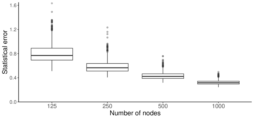
Figure 3: The statistical error $|\!|\widetilde{\bm{\theta}}-{\rm Nature}^{\star}|\!|_{\infty}$ of maximum pseudo-likelihood estimator $\widetilde{\bm{\theta}}$ as an estimator of ${\rm Nature}^{\star}\in\mathbb{R}^{N+1}$ plotted against the number of nodes $N$.

We study the performance of maximum pseudo-likelihood estimators by considering populations with $N=$ 125, 250, 500, and 1,000 nodes. We focus on maximum pseudo-likelihood estimators, because computing maximum likelihood and Monte Carlo maximum likelihood estimators is too time-consuming when $N$ is large (e.g., when $N=500$ and $N=$ 1,000). For each value of $N$, we generate 1,000 populations with overlapping subpopulations as follows:

• The number of subpopulations $K$ is $N\,/\,25$.

• Each node $i\in\mathscr{N}$ belongs to $1+Y_{i}$ subpopulations, where$Y_{i}\;\mathop{\rm\sim}\limits^{\mbox{\tiny iid}}\;\mbox{Binomial}(K-1,\;1\,/\,K)$ ($i=1,\dots,N$).

• For node $i\in\{1,\dots,N\}$, the $1+Y_{i}$ subpopulation memberships are sampled from the Multinomial$(p_{1}^{(i)},\dots,p_{K}^{(i)})$ distribution with

  $$\begin{array}[]{lllllllllllll}p_{k}^{(i)}&=&\begin{cases}\dfrac{1}{K}&\mbox{ if }i=1\vspace{0.25cm}\\ \dfrac{1}{K-1}\;\left(1-\dfrac{N_{k}^{(i-1)}}{N_{1}^{(i-1)}+\ldots+N_{K}^{(i-1)}}\right)&\mbox{ if }i\in\{2,\dots,N\},\end{cases}\end{array}$$

  where $N_{k}^{(i-1)}$ is the number of nodes in $\{1,\dots,i-1\}$ that belong to subpopulation $\mathscr{A}_{k}$ ($k=1,\dots,K$) at the current time.

We consider Model 2 with degree parameters $\theta_{1}^{\star},\ldots,\theta_{N}^{\star}$ drawn fromUniform($-1.25,\,-.75$) and brokerage parameter $\theta_{N+1}^{\star}=.25$. For each population size $N\in\{125,250,500,1000\}$, we generate a graph from Model 2 and compute the maximum pseudo-likelihood estimator from the generated graph. For each value of $N$, the gradient ascent algorithm used to compute the maximum pseudo-likelihood estimator converged for at least 95% of the simulated data sets, and the following simulation results are based on the simulated data sets for which the gradient ascent algorithm converged.

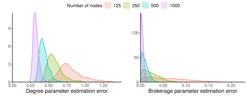
Figure 4: The maximum deviation $\max_{1\leq i\leq N}|\widetilde{\theta}_{i}-\theta_{i}^{\star}|$ of the maximum pseudo-likelihood estimators $\widetilde{\theta}_{i}$ from the data-generating degree parameters $\theta_{i}^{\star}$ ($i=1,\dots,N$) (left) and the deviation $|\widetilde{\theta}_{N+1}-\theta_{N+1}^{\star}|$ of the maximum pseudo-likelihood estimator $\widetilde{\theta}_{N+1}$ from the data-generating brokerage parameter $\theta_{N+1}^{\star}$ (right).

Figure 3 demonstrates that the statistical error $|\!|\widetilde{\bm{\theta}}-{\rm Nature}^{\star}|\!|_{\infty}$ of $\widetilde{\bm{\theta}}$ as an estimator of the data-generating parameter vector ${\rm Nature}^{\star}\in\mathbb{R}^{N+1}$ decreases as the number of nodes $N$ increases. Figure 4 decomposes the statistical error of $\widetilde{\bm{\theta}}$ into the statistical error of the degree parameter estimators $\widetilde{\theta}_{1},\dots,\widetilde{\theta}_{N}$ and the statistical error of the brokerage parameter estimator $\widetilde{\theta}_{N+1}$. Figure 4 reveals that the brokerage parameter is estimated with greater accuracy than the degree parameters, which makes sense as the degree parameters are greater in absolute value than the brokerage parameter and there are $N$ estimated degree parameters $\widetilde{\theta}_{1},\ldots,\widetilde{\theta}_{N}$, compared with the single estimated brokerage parameter $\widetilde{\theta}_{N+1}$.

References

- Amini et al. [2013] Amini, A. A., Chen, A., Bickel, P. J., and Levina, E. (2013), “Pseudo-likelihood methods for community detection in large sparse networks,” The Annals of Statistics, 41, 2097–2122.
- Bhattacharya and Mukherjee [2018] Bhattacharya, B. B., and Mukherjee, S. (2018), “Inference in Ising models,” Bernoulli, 24, 493–525.
- Bickel and Chen [2009] Bickel, P. J., and Chen, A. (2009), “A nonparametric view of network models and Newman-Girvan and other modularities,” in Proceedings of the National Academy of Sciences, Vol. 106, pp. 21068–21073.
- Bollobás et al. [2001] Bollobás, B., Riordan, O., Spencer, J., and Tusnády, G. (2001), “The degree sequence of a scale-free random graph process,” Random Structures & Algorithms, 18, 279–290.
- Brown [1986] Brown, L. (1986), Fundamentals of Statistical Exponential Families: With Applications in Statistical Decision Theory, Hayworth, CA, USA: Institute of Mathematical Statistics.
- Caron and Fox [2017] Caron, F., and Fox, E. B. (2017), “Sparse graphs using exchangeable random measures,” Journal of the Royal Statistical Society, Series B (with discussion), 79, 1–44.
- Chatterjee [2007] Chatterjee, S. (2007), “Estimation in spin glasses: A first step,” The Annals of Statistics, 35, 1931–1946.
- Chatterjee and Diaconis [2013] Chatterjee, S., and Diaconis, P. (2013), “Estimating and understanding exponential random graph models,” The Annals of Statistics, 41, 2428–2461.
- Chatterjee et al. [2011] Chatterjee, S., Diaconis, P., and Sly, A. (2011), “Random graphs with a given degree sequence,” The Annals of Applied Probability, 21, 1400–1435.
- Chazottes et al. [2007] Chazottes, J. R., Collet, P., Külske, C., and Redig, F. (2007), “Concentration inequalities for random fields via coupling,” Probability Theory and Related Fields, 137, 201–225.
- Chen et al. [2021] Chen, M., Kato, K., and Leng, C. (2021), “Analysis of networks via the sparse -model,” Journal of the Royal Statistical Society, Series B (Statistical Methodology), 83, 887–910.
- Comets [1992] Comets, F. (1992), “On consistency of a class of estimators for exponential families of Markov random fields on the lattice,” The Annals of Statistics, 20, 455–468.
- Crane and Dempsey [2018] Crane, H., and Dempsey, W. (2018), “Edge exchangeable models for interaction networks,” Journal of the American Statistical Association, 113, 1311–1326.
- Dawid [1979] Dawid, A. P. (1979), “Conditional independence in statistical theory,” Journal of the Royal Statistical Society, Series B, 41, 1–31.
- Frank and Strauss [1986] Frank, O., and Strauss, D. (1986), “Markov graphs,” Journal of the American Statistical Association, 81, 832–842.
- Furi and Martelli [1991] Furi, M., and Martelli, M. (1991), “On the mean value theorem, inequality, and inclusion,” The American Mathematical Monthly, 98, 840–846.
- Gao et al. [2018] Gao, C., Ma, Z., Zhang, A. Y., and Zhou, H. H. (2018), “Community detection in degree-corrected block models,” The Annals of Statistics, 46, 2153–2185.
- Ghosal and Mukherjee [2020] Ghosal, P., and Mukherjee, S. (2020), “Joint estimation of parameters in Ising model,” The Annals of Statistics, 48, 785–810.
- Handcock [2003] Handcock, M. S. (2003), “Statistical Models for Social Networks: Inference and Degeneracy,” in Dynamic Social Network Modeling and Analysis: Workshop Summary and Papers, eds. Breiger, R., Carley, K., and Pattison, P., Washington, D.C.: National Academies Press, pp. 1–12.
- Harville [1997] Harville, D. A. (1997), Matrix algebra from a statistician’s perspective, New York: Springer.
- Hillar and Wibisono [2015] Hillar, C. J., and Wibisono, A. (2015), “A Hadamard-type lower bound for symmetric diagonally dominant positive matrices,” Linear Algebra and its Applications, 472, 135–141.
- Hoff et al. [2002] Hoff, P. D., Raftery, A. E., and Handcock, M. S. (2002), “Latent space approaches to social network analysis,” Journal of the American Statistical Association, 97, 1090–1098.
- Holland and Leinhardt [1981] Holland, P. W., and Leinhardt, S. (1981), “An exponential family of probability distributions for directed graphs,” Journal of the American Statistical Association, 76, 33–65.
- Karwa and Slavković [2016] Karwa, V., and Slavković, A. B. (2016), “Inference using noisy degrees: Differentially private -model and synthetic graphs,” The Annals of Statistics, 44, 87–112.
- Lauritzen et al. [2018] Lauritzen, S., Rinaldo, A., and Sadeghi, K. (2018), “Random networks, graphical models and exchangeability,” Journal of the Royal Statistical Society: Series B (Statistical Methodology), 80, 481–508.
- Lehmann and Romano [2005] Lehmann, E. L., and Romano, J. P. (2005), Testing Statistical Hypotheses, New York: Springer-Verlag, 3rd ed.
- Lindvall [2002] Lindvall, T. (2002), Lectures On The Coupling Method, Courier Corporation.
- Mukherjee et al. [2018] Mukherjee, R., Mukherjee, S., and Sen, S. (2018), “Detection thresholds for the -model on sparse graphs,” The Annals of Statistics, 46, 1288–1317.
- Mukherjee [2020] Mukherjee, S. (2020), “Degeneracy in sparse ERGMs with functions of degrees as sufficient statistics,” Bernoulli, 26, 1016–1043.
- Portnoy [1988] Portnoy, S. (1988), “Asymptotic behavior of likelihood methods for exponential families when the number of parameters tends to infinity,” The Annals of Statistics, 16, 356–366.
- Ravikumar et al. [2010] Ravikumar, P., Wainwright, M. J., and Lafferty, J. (2010), “High-dimensional Ising model selection using -regularized logistic regression,” The Annals of Statistics, 38, 1287–1319.
- Rinaldo et al. [2009] Rinaldo, A., Fienberg, S. E., and Zhou, Y. (2009), “On the geometry of discrete exponential families with application to exponential random graph models,” Electronic Journal of Statistics, 3, 446–484.
- Rinaldo et al. [2013] Rinaldo, A., Petrović, S., and Fienberg, S. E. (2013), “Maximum likelihood estimation in the -model,” The Annals of Statistics, 41, 1085–1110.
- Rohe et al. [2011] Rohe, K., Chatterjee, S., and Yu, B. (2011), “Spectral clustering and the high-dimensional stochastic block model,” The Annals of Statistics, 39, 1878–1915.
- Schweinberger [2011] Schweinberger, M. (2011), “Instability, sensitivity, and degeneracy of discrete exponential families,” Journal of the American Statistical Association, 106, 1361–1370.
- Schweinberger et al. [2020] Schweinberger, M., Krivitsky, P. N., Butts, C. T., and Stewart, J. R. (2020), “Exponential-family models of random graphs: Inference in finite, super, and infinite population scenarios,” Statistical Science, 35, 627–662.
- Schweinberger and Stewart [2020] Schweinberger, M., and Stewart, J. R. (2020), “Concentration and consistency results for canonical and curved exponential-family models of random graphs,” The Annals of Statistics, 48, 374–396.
- Stewart and Schweinberger [2023] Stewart, J. R., and Schweinberger, M. (2023), “Supplement to: Pseudo-likelihood-based -estimators for random graphs with dependent edges and parameter vectors of increasing dimension,” Department of Statistics, Florida State University.
- van den Berg and Maes [1994] van den Berg, J., and Maes, C. (1994), “Disagreement percolation in the study of Markov fields,” The Annals of Probability, 22, 749–763.
- Watts [2003] Watts, D. J. (2003), Six Degrees. The Science of a Connected Age, Norton.
- Yan et al. [2016] Yan, T., Leng, C., and Zhu, J. (2016), “Asymptotics in directed exponential random graph models with an increasing bi-degree sequence,” The Annals of Statistics, 44, 31–57.
- Yan and Xu [2013] Yan, T., and Xu, J. (2013), “A central limit theorem in the -model for undirected random graphs with a diverging number of vertices,” Biometrika, 100, 519–524.
Supplement to:

References

- Amini et al. [2013] Amini, A. A., Chen, A., Bickel, P. J., and Levina, E. (2013), “Pseudo-likelihood methods for community detection in large sparse networks,” The Annals of Statistics, 41, 2097–2122.
- Bhattacharya and Mukherjee [2018] Bhattacharya, B. B., and Mukherjee, S. (2018), “Inference in Ising models,” Bernoulli, 24, 493–525.
- Bickel and Chen [2009] Bickel, P. J., and Chen, A. (2009), “A nonparametric view of network models and Newman-Girvan and other modularities,” in Proceedings of the National Academy of Sciences, Vol. 106, pp. 21068–21073.
- Bollobás et al. [2001] Bollobás, B., Riordan, O., Spencer, J., and Tusnády, G. (2001), “The degree sequence of a scale-free random graph process,” Random Structures & Algorithms, 18, 279–290.
- Brown [1986] Brown, L. (1986), Fundamentals of Statistical Exponential Families: With Applications in Statistical Decision Theory, Hayworth, CA, USA: Institute of Mathematical Statistics.
- Caron and Fox [2017] Caron, F., and Fox, E. B. (2017), “Sparse graphs using exchangeable random measures,” Journal of the Royal Statistical Society, Series B (with discussion), 79, 1–44.
- Chatterjee [2007] Chatterjee, S. (2007), “Estimation in spin glasses: A first step,” The Annals of Statistics, 35, 1931–1946.
- Chatterjee and Diaconis [2013] Chatterjee, S., and Diaconis, P. (2013), “Estimating and understanding exponential random graph models,” The Annals of Statistics, 41, 2428–2461.
- Chatterjee et al. [2011] Chatterjee, S., Diaconis, P., and Sly, A. (2011), “Random graphs with a given degree sequence,” The Annals of Applied Probability, 21, 1400–1435.
- Chazottes et al. [2007] Chazottes, J. R., Collet, P., Külske, C., and Redig, F. (2007), “Concentration inequalities for random fields via coupling,” Probability Theory and Related Fields, 137, 201–225.
- Chen et al. [2021] Chen, M., Kato, K., and Leng, C. (2021), “Analysis of networks via the sparse -model,” Journal of the Royal Statistical Society, Series B (Statistical Methodology), 83, 887–910.
- Comets [1992] Comets, F. (1992), “On consistency of a class of estimators for exponential families of Markov random fields on the lattice,” The Annals of Statistics, 20, 455–468.
- Crane and Dempsey [2018] Crane, H., and Dempsey, W. (2018), “Edge exchangeable models for interaction networks,” Journal of the American Statistical Association, 113, 1311–1326.
- Dawid [1979] Dawid, A. P. (1979), “Conditional independence in statistical theory,” Journal of the Royal Statistical Society, Series B, 41, 1–31.
- Frank and Strauss [1986] Frank, O., and Strauss, D. (1986), “Markov graphs,” Journal of the American Statistical Association, 81, 832–842.
- Furi and Martelli [1991] Furi, M., and Martelli, M. (1991), “On the mean value theorem, inequality, and inclusion,” The American Mathematical Monthly, 98, 840–846.
- Gao et al. [2018] Gao, C., Ma, Z., Zhang, A. Y., and Zhou, H. H. (2018), “Community detection in degree-corrected block models,” The Annals of Statistics, 46, 2153–2185.
- Ghosal and Mukherjee [2020] Ghosal, P., and Mukherjee, S. (2020), “Joint estimation of parameters in Ising model,” The Annals of Statistics, 48, 785–810.
- Handcock [2003] Handcock, M. S. (2003), “Statistical Models for Social Networks: Inference and Degeneracy,” in Dynamic Social Network Modeling and Analysis: Workshop Summary and Papers, eds. Breiger, R., Carley, K., and Pattison, P., Washington, D.C.: National Academies Press, pp. 1–12.
- Harville [1997] Harville, D. A. (1997), Matrix algebra from a statistician’s perspective, New York: Springer.
- Hillar and Wibisono [2015] Hillar, C. J., and Wibisono, A. (2015), “A Hadamard-type lower bound for symmetric diagonally dominant positive matrices,” Linear Algebra and its Applications, 472, 135–141.
- Hoff et al. [2002] Hoff, P. D., Raftery, A. E., and Handcock, M. S. (2002), “Latent space approaches to social network analysis,” Journal of the American Statistical Association, 97, 1090–1098.
- Holland and Leinhardt [1981] Holland, P. W., and Leinhardt, S. (1981), “An exponential family of probability distributions for directed graphs,” Journal of the American Statistical Association, 76, 33–65.
- Karwa and Slavković [2016] Karwa, V., and Slavković, A. B. (2016), “Inference using noisy degrees: Differentially private -model and synthetic graphs,” The Annals of Statistics, 44, 87–112.
- Lauritzen et al. [2018] Lauritzen, S., Rinaldo, A., and Sadeghi, K. (2018), “Random networks, graphical models and exchangeability,” Journal of the Royal Statistical Society: Series B (Statistical Methodology), 80, 481–508.
- Lehmann and Romano [2005] Lehmann, E. L., and Romano, J. P. (2005), Testing Statistical Hypotheses, New York: Springer-Verlag, 3rd ed.
- Lindvall [2002] Lindvall, T. (2002), Lectures On The Coupling Method, Courier Corporation.
- Mukherjee et al. [2018] Mukherjee, R., Mukherjee, S., and Sen, S. (2018), “Detection thresholds for the -model on sparse graphs,” The Annals of Statistics, 46, 1288–1317.
- Mukherjee [2020] Mukherjee, S. (2020), “Degeneracy in sparse ERGMs with functions of degrees as sufficient statistics,” Bernoulli, 26, 1016–1043.
- Portnoy [1988] Portnoy, S. (1988), “Asymptotic behavior of likelihood methods for exponential families when the number of parameters tends to infinity,” The Annals of Statistics, 16, 356–366.
- Ravikumar et al. [2010] Ravikumar, P., Wainwright, M. J., and Lafferty, J. (2010), “High-dimensional Ising model selection using -regularized logistic regression,” The Annals of Statistics, 38, 1287–1319.
- Rinaldo et al. [2009] Rinaldo, A., Fienberg, S. E., and Zhou, Y. (2009), “On the geometry of discrete exponential families with application to exponential random graph models,” Electronic Journal of Statistics, 3, 446–484.
- Rinaldo et al. [2013] Rinaldo, A., Petrović, S., and Fienberg, S. E. (2013), “Maximum likelihood estimation in the -model,” The Annals of Statistics, 41, 1085–1110.
- Rohe et al. [2011] Rohe, K., Chatterjee, S., and Yu, B. (2011), “Spectral clustering and the high-dimensional stochastic block model,” The Annals of Statistics, 39, 1878–1915.
- Schweinberger [2011] Schweinberger, M. (2011), “Instability, sensitivity, and degeneracy of discrete exponential families,” Journal of the American Statistical Association, 106, 1361–1370.
- Schweinberger et al. [2020] Schweinberger, M., Krivitsky, P. N., Butts, C. T., and Stewart, J. R. (2020), “Exponential-family models of random graphs: Inference in finite, super, and infinite population scenarios,” Statistical Science, 35, 627–662.
- Schweinberger and Stewart [2020] Schweinberger, M., and Stewart, J. R. (2020), “Concentration and consistency results for canonical and curved exponential-family models of random graphs,” The Annals of Statistics, 48, 374–396.
- Stewart and Schweinberger [2023] Stewart, J. R., and Schweinberger, M. (2023), “Supplement to: Pseudo-likelihood-based -estimators for random graphs with dependent edges and parameter vectors of increasing dimension,” Department of Statistics, Florida State University.
- van den Berg and Maes [1994] van den Berg, J., and Maes, C. (1994), “Disagreement percolation in the study of Markov fields,” The Annals of Probability, 22, 749–763.
- Watts [2003] Watts, D. J. (2003), Six Degrees. The Science of a Connected Age, Norton.
- Yan et al. [2016] Yan, T., Leng, C., and Zhu, J. (2016), “Asymptotics in directed exponential random graph models with an increasing bi-degree sequence,” The Annals of Statistics, 44, 31–57.
- Yan and Xu [2013] Yan, T., and Xu, J. (2013), “A central limit theorem in the -model for undirected random graphs with a diverging number of vertices,” Biometrika, 100, 519–524.