Phase transitions in the frustrated Ising ladder with stoquastic and nonstoquastic catalysts

Abstract

The role of nonstoquasticity in the field of quantum annealing and adiabatic quantum computing is an actively debated topic. We study a strongly-frustrated quasi-one-dimensional quantum Ising model on a two-leg ladder to elucidate how a first-order phase transition with a topological origin is affected by interactions of the $\pm XX$-type. Such interactions are sometimes known as stoquastic (negative sign) and nonstoquastic (positive sign) “catalysts”. Carrying out a symmetry-preserving real-space renormalization group analysis and extensive density-matrix renormalization group computations, we show that the phase diagrams obtained by these two methods are in qualitative agreement with each other and reveal that the first-order quantum phase transition of a topological nature remains stable against the introduction of both $XX$-type catalysts. This is the first study of the effects of nonstoquasticity on a first-order phase transition between topologically distinct phases. Our results indicate that nonstoquastic catalysts are generally insufficient for removing topological obstacles in quantum annealing and adiabatic quantum computing.

I Introduction

Quantum annealing exploits quantum-mechanical fluctuations to solve combinatorial optimization problems Kadowaki and Nishimori (1998); Brooke et al. (1999); Farhi et al. (2001); Santoro et al. (2002); Santoro and Tosatti (2006); Morita and Nishimori (2008); Albash and Lidar (2018); Hauke et al. (2020). In a typical formulation, the combinatorial optimization problem one wants to solve is expressed as an Ising model, represented in terms of the $z$ components of the Pauli matrices, and quantum fluctuations are introduced as a transverse field (sometimes called the $X$ term), the sum of the $x$ components of the Pauli matrices over all sites. One of the bottlenecks of quantum annealing under unitary Schrödinger dynamics is a first-order quantum phase transition as a function of the relative weight of the Ising Hamiltonian and the $X$ term, which exists in almost all cases of interest. At a first-order quantum phase transition, the energy gap between the ground state and the first excited state closes exponentially as a function of the system size except for a few very limited cases Tsuda et al. (2013); Pfeuty (1970); Laumann et al. (2012). This leads to exponentially long computation times within the framework of adiabatic time evolution, according to the adiabatic theorem of quantum mechanics Jansen et al. (2007); Mozgunov and Lidar (2020). There has been a large amount of effort to circumvent this difficulty including, but not limited to, the introduction of nonstoquastic catalysts Farhi et al. (2002); Seki and Nishimori (2012); Seoane and Nishimori (2012); Crosson et al. (2014); Seki and Nishimori (2015); Hormozi et al. (2017); Nishimori and Takada (2017); Albash (2019); Takada et al. (2020); Matsuura et al. (2021); Crosson et al. (2020), inhomogeneous field driving Farhi et al. (2011); Dickson and Amin (2011, 2012); Susa et al. (2018a); Mohseni et al. (2018); Susa et al. (2018b); Adame and McMahon (2020), reverse annealing Perdomo-Ortiz et al. (2010); Chancellor (2017); Ohkuwa et al. (2018); Yamashiro et al. (2019); King et al. (2018); Ottaviani and Amendola (2018); Marshall et al. (2019); Venturelli and Kondratyev (2019); Ikeda et al. (2019); Rocutto et al. (2021); Passarelli et al. (2020); Arai et al. (2021), pausing Marshall et al. (2019); Passarelli et al. (2019); Kadowaki and Ohzeki (2019); Chen and Lidar (2020), and diabatic quantum annealing Crosson and Lidar (2021). In the present paper, we focus on the approach of nonstoquastic catalysts.

A Hamiltonian is called stoquastic if there is a choice of a local (tensor-product) basis in which the Hamiltonian off-diagonal matrix elements are all real and nonpositive Bravyi et al. (2008). Otherwise the Hamiltonian is called nonstoquastic, and the inevitable positive or complex off-diagonal matrix elements of the Hamiltonian lead to the infamous sign problem Loh et al. (1990); Gupta and Hen (2019). We note that even when the Hamiltonian is stoquastic, but it is presented in a form in which this stoquasticity is unapparent, the problem of deciding whether there exists a local transformation to a basis that “cures the sign problem” (makes it stoquastic) by making all of the Hamiltonian matrix elements real and nonpositive, is NP-complete Marvian et al. (2019); Klassen et al. (2020).

Many interesting quantum models are stoquastic, e.g., the transverse-field Ising model of conventional quantum annealing, the Bose-Hubbard model, and particles subject to a position-dependent potential, which includes superconducting flux circuits if we associate flux with position and charge with momentum Bravyi et al. (2008); Halverson et al. (2020). The partition-function decomposition of a stoquastic Hamiltonian leads to a sum of nonnegative weights (i.e., the absence of sign problem, which means that the path-integral quantum Monte Carlo algorithm Suzuki (1976) can typically be used efficiently for sampling tasks). Moreover, the ground state of a stoquastic Hamiltonian has only nonnegative amplitudes by the Perron-Frobenius theorem. These two observations are often cited as reasons that stoquastic Hamiltonians should be considered to be less computationally powerful than their nonstoquastic counterparts. In addition, it is well known that nonstoquastic adiabatic quantum computation is universal Aharonov et al. (2007); Mizel et al. (2007); Gosset et al. (2015), while universality in the stoquastic case requires excited states Jordan et al. (2010). From a computational complexity perspective, the class StoqMA associated with the task of estimating the ground-state energy of stoquastic local Hamiltonians is known to be no harder than QMA and no easier than MA (and hence no easier than NP) Bravyi et al. (2006) (see Ref. Albash and Lidar (2018) for more background).

However, recently evidence has been mounting that nonstoquasticity does not have a clear-cut computational benefit even in the ground state setting. For example, very recently examples were found for which evolution in the ground state of a stoquastic Hamiltonian can solve a problem superpolynomially Hastings (2020) or even subexponentially Gilyén et al. (2021) faster than is possible classically. In addition, there is both theoretical and numerical evidence that adiabatic paths based on nonstoquastic Hamiltonians generically have smaller gaps between the ground state and the first excited state, with the implication that they are less useful than stoquastic Hamiltonians for adiabatic quantum optimization Crosson et al. (2020). In this work we contribute further evidence that nonstoquasticity is not necessarily useful for efficiently solving a problem.

The setting for our work is the conventional transverse-field Ising model used in quantum annealing, but with added antiferromagnetic $XX$ interactions ($XX$ terms with positive coefficients). Such terms, which can turn a stoquastic Hamiltonian into a nonstoquastic one, are sometimes called nonstoquastic “catalysts” when they are turned on only at intermediate times (typically as $s(1-s)$, where $s\in[0,1]$ is the dimensionless time along the anneal) Albash and Lidar (2018); Albash (2019), a terminology inspired by its use in entanglement theory Jonathan and Plenio (1999).

One of the outstanding features of the introduction of an $XX$-type nonstoquastic catalyst lies in the universality and QMA-completeness of the resulting Hamiltonian, assuming independent control of each term in the Hamiltonian Biamonte and Love (2008). Our focus is, however, on another aspect, namely, that a certain set of nonstoquastic catalysts of the $XX$ type is known to reduce the order of quantum phase transitions from first to second Seki and Nishimori (2012); Seoane and Nishimori (2012); Seki and Nishimori (2015); Nishimori and Takada (2017); Albash (2019); Takada et al. (2020). This means that adiabatic evolution converges to the ground state of the final Hamiltonian in quantum annealing with an exponential speedup relative to the stoquastic case. However, it does not guarantee a quantum speedup relative to classical solution methods, and in addition examples are known where $XX$-type nonstoquastic catalysts do not lead to performance improvements Hormozi et al. (2017); Farhi et al. (2011); Takada et al. (2020); Crosson et al. (2020). All of these studies concern problems with relatively simple phase transitions without a drastic change in the topological structure of thermodynamic phases.

The frustrated ladder model introduced by Laumann et al. Laumann et al. (2012) is an exceptional case in that it undergoes a first-order quantum phase transition between topologically different phases despite the simplicity of the problem, which is defined on a quasi-one-dimensional two-leg ladder with nearest-neighbor interactions. The model is closely related to a dimer problem defined on a dual ladder, through which the topological aspect of its phase transition can be understood intuitively, as will be detailed in Sec. II. For this reason, we study the effects of nonstoquastic $XX$ catalysts on the phase transition of the frustrated Ising ladder, and the stoquastic case is also treated for completeness.

We employ theoretical and numerical tools, i.e., the real-space renormalization group (RG) method and the density-matrix renormalization group (DMRG) method, to study the structure of the phase diagram with and without $XX$ catalysts of both signs (stoquastic and nonstoquastic). We find that the phase diagrams obtained by the two methods are qualitatively consistent with each other and conclude that the $XX$-type catalysts, both stoquastic and nonstoquastic, keep the order of the phase transition intact. This is the first example where the role of stoquastic and nonstoquastic catalysts is revealed systematically in a low-dimensional system that exhibits a first-order phase transition with a change of the topological structure.

This paper is organized as follows: In the next section we formulate the problem and describe the known properties of the model system. In Sec. III we analyze the problem via the real-space RG method. The results of extensive numerical computations are explained in Sec. IV and are compared with those from the real-space RG method. We conclude in Sec. V. Additional technical details are given in the Appendices.

II Model

We consider the frustrated Ising ladder with transverse fields and $XX$ interactions. This is a generalization of the model proposed and analyzed in Ref. Laumann et al. (2012), where the transverse field was uniformly applied to all sites and no $XX$ interactions were taken into account. This section describes the definition of the model and its basic properties in the case without $XX$ interactions, and is largely a recapitulation of Ref. Laumann et al. (2012).

II.1 Definition of the model

As depicted in Fig. 1, the system is composed of qubits (spin-1/2 particles) located on sites of a two-leg ladder. The ladder has a top row ($\mathrm{t}$) and a bottom row ($\mathrm{b}$). Nearest-neighbor interactions are of magnitude $K>0$ with ferromagnetic (solid lines) or antiferromagnetic (dashed lines) signs. Local longitudinal fields applied to the top and bottom rows have magnitudes $K$ and $U/2>0$, respectively, and are oppositely directed. With transverse fields ($X$ terms) of magnitude $\Gamma_{\mathrm{t}}$ or $\Gamma_{\mathrm{b}}$ and transverse interactions ($XX$ terms) with magnitude $\Xi_{\mathrm{t}\mathrm{t}}$, $\Xi_{\mathrm{t}\mathrm{b}}$, or $\Xi_{\mathrm{b}\mathrm{b}}$, the Hamiltonian is written as

$$\hat{H} =\sum_{i=1}^{L}\biggl{[}K(\hat{Z}_{\mathrm{t},i}\hat{Z}_{\mathrm{t},i+1}-\hat{Z}_{\mathrm{b},i}\hat{Z}_{\mathrm{b},i+1}-\hat{Z}_{\mathrm{t},i}\hat{Z}_{\mathrm{b},i}-\hat{Z}_{\mathrm{t},i})$$

$$\hphantom{{}=\sum\biggl{[}}+\frac{U}{2}\hat{Z}_{\mathrm{b},i}-(\Gamma_{\mathrm{t}}\hat{X}_{\mathrm{t},i}+\Gamma_{\mathrm{b}}\hat{X}_{\mathrm{b},i})$$

$$\hphantom{{}=\sum\biggl{[}}-(\Xi_{\mathrm{t}\mathrm{t}}\hat{X}_{\mathrm{t},i}\hat{X}_{\mathrm{t},i+1}+\Xi_{\mathrm{b}\mathrm{b}}\hat{X}_{\mathrm{b},i}\hat{X}_{\mathrm{b},i+1}$$

$$\hphantom{{}=\sum\biggl{[}-(}+\Xi_{\mathrm{t}\mathrm{b}}\hat{X}_{\mathrm{t},i}\hat{X}_{\mathrm{b},i})\biggr{]},$$ (1)

where $\hat{X}_{a,i}$, $\hat{Y}_{a,i}$, and $\hat{Z}_{a,i}$ are the Pauli operators at sites $i=1,\dots,L$ on row $a=\mathrm{t},\mathrm{b}$. We assume the length $L$ to be even and impose the periodic boundary conditions

$$\hat{X}_{a,L+1}=\hat{X}_{a,1},\quad\hat{Y}_{a,L+1}=\hat{Y}_{a,1},\quad\hat{Z}_{a,L+1}=\hat{Z}_{a,1}.$$ (2)

The classical part of $\hat{H}$ (the terms involving $Z$ operators) is highly frustrated due to the competition between positive and negative interactions as well as between interactions and longitudinal fields.

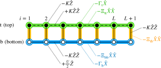
Figure 1: Frustrated Ising ladder with transverse fields and $XX$ interactions. Spin-$1/2$ particles are located at the black circles on the top row and white circles on the bottom row. The black solid lines are ferromagnetic interactions of magnitude $K$ and the black dashed lines are antiferromagnetic interactions of magnitude $K$. Local longitudinal fields $K$ and $U/2$ are applied at each black circle and each white circle, respectively, and have opposite directions. A transverse field $\Gamma_{\mathrm{t}}$ is appended at every site on the top row and $\Gamma_{\mathrm{b}}$ on the bottom row. An $XX$ interaction $\Xi_{\mathrm{t}\mathrm{t}}$ is applied on each horizontal bond on the top row, $\Xi_{\mathrm{b}\mathrm{b}}$ on each horizontal bond on the bottom row, and $\Xi_{\mathrm{t}\mathrm{b}}$ on each vertical bond between the two rows. The interactions and fields are indicated by operators in the figure, where the subscripts of the Pauli operators $\hat{X}_{a,i}$, $\hat{Y}_{a,i}$, and $\hat{Z}_{a,i}$ are omitted. Periodic boundary conditions are imposed by identifying the sites at the horizontal position $i=L+1$ with those at $i=1$.

Let us discuss the stoquasticity of the Hamiltonian $\hat{H}$. As is easily checked, $\hat{H}$ is stoquastic for $\Xi_{\mathrm{t}\mathrm{t}},\Xi_{\mathrm{b}\mathrm{b}},\Xi_{\mathrm{t}\mathrm{b}}\geq 0$. Additionally, when $\Xi_{\mathrm{t}\mathrm{t}}<0$, $\Xi_{\mathrm{b}\mathrm{b}}<0$, or $\Xi_{\mathrm{t}\mathrm{b}}<0$, there are cases where a local curing transformation makes the Hamiltonian stoquastic. For example, if $\Gamma_{\mathrm{t}}=\Gamma_{\mathrm{b}}=0$ and $\Xi_{\mathrm{t}\mathrm{t}},\Xi_{\mathrm{b}\mathrm{b}},\Xi_{\mathrm{t}\mathrm{b}}\leq 0$, consider the transformation obtained by conjugating some qubits by $\hat{Z}_{a,i}$, an operation under which $\hat{X}_{a,i}\mapsto-\hat{X}_{a,i}$. Then, the following is a curing transformation: for odd $i$, conjugate the qubits on the top row and for even $i$, conjugate the bottom row. This transformation is equivalent to flipping the signs of $\Xi_{\mathrm{t}\mathrm{t}}$, $\Xi_{\mathrm{b}\mathrm{b}}$, and $\Xi_{\mathrm{t}\mathrm{b}}$ when $\Gamma_{\mathrm{t}}=\Gamma_{\mathrm{b}}=0$.

It can be shown Takada and Lidar that $\hat{H}$ remains nonstoquastic under single-qubit Clifford transformations if the following set of conditions is satisfied:

$$\left\{\begin{aligned} &\Gamma_{\mathrm{t}},\Gamma_{\mathrm{b}}>0,\\ &\Xi_{\mathrm{t}\mathrm{t}}<0\vee\Xi_{\mathrm{b}\mathrm{b}}<0\vee\Xi_{\mathrm{t}\mathrm{b}}<0,\\ &\lvert U/2\rvert,\lvert\Xi_{\mathrm{t}\mathrm{b}}\rvert<K.\end{aligned}\right.$$ (3)

Since the general problem of deciding whether a local curing transformation exists is NP-complete even for single-qubit Clifford transformations Marvian et al. (2019); Klassen et al. (2020), we do not consider here the nonstoquasticity of $\hat{H}$ in more general cases than the conditions given by Eq. (3). In the following, we refer to $\hat{H}$ as nonstoquastic if there is no curing transformation that is a product of single-qubit Clifford unitaries, and as stoquastic otherwise.

II.2 Phase diagram for the case without $XX$ terms

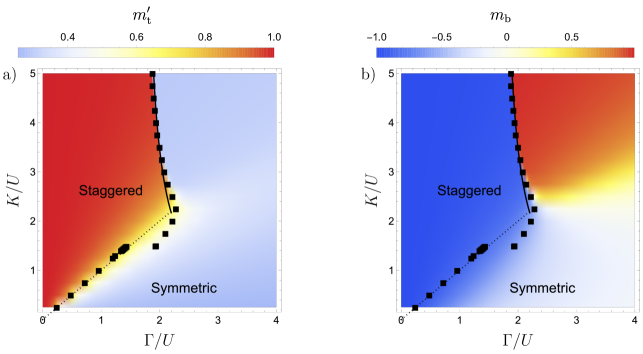
Figure 2: Phase diagram of the Ising ladder with uniform transverse field $\Gamma$ and no $XX$ terms, where the staggered magnetization of the top row $m^{\prime}_{\mathrm{t}}$ is color-coded in (a) and the magnetization of the bottom row $m_{\mathrm{b}}$ in (b). The black squares in (a) and (b) are the locations of the minimum energy gap for fixed values of $K/U$. Here, we set the system size to $L=10$. In both of (a) and (b), the first- and second-order phase boundaries predicted by perturbation theory are shown as solid and dotted lines, respectively. The first-order transition line for $K/U\gg 1$ is $\Gamma/U\approx 1/c+U/(4Kc^{3})$ ($c\approx 0.6$) and the second-order transition line for $K/U\ll 1$ is $\Gamma/U\approx K/U$ Laumann et al. (2012).

Laumann et al. Laumann et al. (2012) studied the phase diagram in the case of the uniform transverse field $\Gamma_{\mathrm{t}}=\Gamma_{\mathrm{b}}=\Gamma$ and no $XX$ interactions $\Xi_{\mathrm{t}\mathrm{t}}=\Xi_{\mathrm{b}\mathrm{b}}=\Xi_{\mathrm{t}\mathrm{b}}=0$ using numerical diagonalization of small-size systems and perturbation from the large-$K$ and small-$K$ limits. We confirm their findings in Fig. 2, which shows that a first-order transition exists as a function of $\Gamma/U$ with $K/U$ fixed to a large value, while a second-order transition appears for small $K/U$. The values of $\Gamma/U$ that minimize the energy gap between the ground state and the first excited state (which we refer to henceforth as “minimum gap points”) for $L=10$ and fixed values of $K/U$ are indicated in Fig. 2 by black squares. According to perturbation theory, the first-order transition line for $K/U\gg 1$ is $\Gamma/U\approx 1/c+U/(4Kc^{3})$ ($c\approx 0.6$) and the second-order transition line for $K/U\ll 1$ is $\Gamma/U\approx K/U$ Laumann et al. (2012). These two lines meet at $(\Gamma/U,K/U)\approx(2.2,2.2)$.

Note that the perturbation theory prediction agrees with the location of the minimum gap points for $K/U\gtrsim 2.2$ or $K/U\lesssim 1.5$, but the agreement breaks down for $1.5\lesssim K/U\lesssim 2.2$, where the numerically computed locations of the minimum gap deviate from the perturbative second-order transition line. A jump in the minimum gap points is observed at $K/U\approx 1.5$ between $\Gamma/U\approx 1.5$ and $1.9$. We provide an explanation of this phenomenon in terms of the appearance of a “double-well” in the energy gap as a function of $\Gamma/U$ at the critical value $K/U\approx 1.5$, which is the origin of the observed discontinuity. See Appendix A for additional details.

Figure 2 also shows the staggered magnetization of the top row

$$m^{\prime}_{\mathrm{t}}=\Braket{\left\lvert\frac{1}{L}\sum_{i=1}^{L}(-1)^{i}\hat{Z}_{\mathrm{t},i}\right\rvert}$$ (4)

and the magnetization of the bottom row

$$m_{\mathrm{b}}=\Braket{\frac{1}{L}\sum_{i=1}^{L}\hat{Z}_{\mathrm{b},i}}$$ (5)

for $L=10$, where $\braket{\cdots}$ denotes the expectation value in the ground state. We see that $m^{\prime}_{\mathrm{t}}$ and $m_{\mathrm{b}}$ have discontinuities as functions of $\Gamma/U$ for large $K/U$, which indicate the existence of the first-order transition. On the other hand, $m^{\prime}_{\mathrm{t}}$ and $m_{\mathrm{b}}$ change continuously around the second-order transition, which occurs as $\Gamma/U$ is decreased with $K/U$ fixed to a small value.

The “symmetric” and “staggered” phases shown in Fig. 2 are associated with columnar and staggered configurations, which are defined as follows:

• Columnar configurations are product states of local eigenstates of $\hat{Z}_{a,i}$ in which all the bottom-row spins are up and there are no nearest-neighbor (consecutive) down spins on the top row.

• Staggered configurations are product states of local eigenstates of $\hat{Z}_{a,i}$ in which all the bottom-row spins are down and nearest-neighbor top-row spins are antiparallel (antiferromagnetically ordered).

When $K$ is large, the two phases can be characterized by perturbation theory in $K^{-1}$. The leading-order part of the state in the symmetric phase is a superposition of columnar configurations (e.g., the red arrows in the top panel of Fig. 3), while that in the staggered phase has staggered configurations (red arrows in the middle and bottom panels of Fig. 3). The name “symmetric phase” means that all columnar spin configurations have comparable amplitudes with the wave function exhibiting translational invariance, and this invariance is broken in the staggered phase. The system is in the symmetric phase for large $\Gamma/U$ and is in the staggered phase for small $\Gamma/U$. Reference Laumann et al. (2012) also verified that the energy gaps at the first-order transition points decay exponentially as the length $L$ grows and that the decay rate is proportional to $\ln(K/\Gamma)$. This can be intuitively understood from the fact that the transition from a columnar configuration to a staggered configuration requires flipping all the bottom spins as shown in Fig. 3.

As reviewed in Appendix B.1, the ground states of the nonperturbative Hamiltonian proportional to $K$,

$$\hat{H}^{(0)}=K\sum_{i=1}^{L}(\hat{Z}_{\mathrm{t},i}\hat{Z}_{\mathrm{t},i+1}-\hat{Z}_{\mathrm{b},i}\hat{Z}_{\mathrm{b},i+1}-\hat{Z}_{\mathrm{t},i}\hat{Z}_{\mathrm{b},i}-\hat{Z}_{\mathrm{t},i}),$$ (6)

are the columnar and staggered configurations. In the presence of the perturbative terms with the coefficients $U$ and $\Gamma$, the degeneracy of $\hat{H}^{(0)}$ is lifted as described above.

The number of columnar configurations is the sum of two Fibonacci numbers $F_{L-1}+F_{L-3}$, which is exponentially large in the length $L$. Here, $F_{L}$ is defined by the recurrence relation $F_{L}=F_{L-1}+F_{L-2}$ and the initial values $F_{1}=2$ and $F_{2}=3$. On the other hand, there are only two staggered configurations. These basic properties are confirmed in Appendix B.1.

In the opposite limit $U\to\infty$, the bottom spins are fixed to down, and the top row of the original Ising ladder (1) with $\Gamma_{\mathrm{t}}=\Gamma_{\mathrm{b}}=\Gamma$ and $\Xi_{\mathrm{t}\mathrm{t}}=\Xi_{\mathrm{b}\mathrm{b}}=\Xi_{\mathrm{t}\mathrm{b}}=0$ is effectively an antiferromagnetic Ising chain in a transverse field, $\sum_{i=1}^{L}(K\hat{Z}_{\mathrm{t},i}\hat{Z}_{\mathrm{t},i+1}-\Gamma\hat{X}_{\mathrm{t},i})$. This results in a second-order transition approximately at $\Gamma=K$ for small $K/U$, as shown in Fig. 2. The symmetric and staggered phases of the ladder correspond to the quantum paramagnetic and antiferromagnetic phases on the top row, respectively.

II.3 Dimer model on the dual lattice

A significant property of the frustrated Ising ladder is that in the limit of large frustration $K\to\infty$ the model is equivalent to the quantum dimer model on a two-leg ladder, as shown in Ref. Laumann et al. (2012). We can find this equivalence by locating dimers on the dual lattice according to the types and positions of frustration exhibited by the columnar and staggered configurations. The dual lattice is a two-leg ladder whose position is shifted horizontally and vertically by half of the unit length from the Ising ladder (see Fig. 3). Types of frustration in the columnar and staggered configurations are classified as (i) a down spin on the top row (opposite to the longitudinal field), (ii) a horizontally aligned ferromagnetic pair on the top row (opposite to the antiferromagnetic interaction), and (iii) a vertically aligned antiferromagnetic pair (opposite to the ferromagnetic interaction). In the dimer picture these three types become (i) a top horizontal dimer, (ii) a vertical dimer, and (iii) a bottom horizontal dimer, respectively. In this manner the columnar and staggered configurations in the frustrated Ising ladder are mapped one-to-one onto hardcore dimer coverings on the dual two-leg ladder.

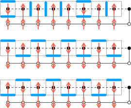
Figure 3: Examples of the correspondence between states in the frustrated Ising model and the dimer model on two-leg ladders. The lattice for the former model is depicted in a similar way to Fig. 1 (namely, the black circles, the black solid lines, and the black dashed lines are longitudinal fields, ferromagnetic interactions, and antiferromagnetic interactions, respectively, of equal magnitude $K$), while the dual lattice for the latter model is indicated by the dotted lines. The rightmost points are identified with the leftmost points for each lattice, which is subject to periodic boundary conditions. The red arrows are spins and the blue thick line segments are dimers. The topological number is $w=0,+1,-1$ from top to bottom, the first being a columnar configuration and the second and the third being staggered ones.

Dimer coverings on a two-leg ladder are classified into three topological sectors: the columnar sector $w=0$ and the two staggered sectors $w=\pm 1$, where $w$ denotes the difference in the number of dimers between the top and bottom rows on an arbitrarily given unit square (plaquette). The fact that one cannot transform a dimer covering into another dimer covering with a different $w$ by a series of local movements of dimers allows us to regard $w$ as a topological number.

From this mapping of the columnar and staggered configurations in the frustrated Ising ladder onto dimer coverings, it follows that the Hamiltonian of the frustrated Ising ladder (1) in the limit $K\to\infty$ is equivalent to the following Hamiltonian of the quantum dimer model:

$$\hat{H}_{\text{dimer}} =U\left(\sum_{|}\Ket{\phantom{\Bigl{\lvert}}|\phantom{\Bigr{\rvert}}}\Bra{\phantom{\Bigl{\lvert}}|\phantom{\Bigr{\rvert}}}+2\sum_{\square}\Ket{\vphantom{\Bigl{\lvert}}=\vphantom{\Bigr{\rvert}}}\Bra{\vphantom{\Bigl{\lvert}}=\vphantom{\Bigr{\rvert}}}\right)$$

$$\hphantom{{}={}}-\Gamma_{\mathrm{t}}\sum_{\square}\left(\Ket{\phantom{\Bigl{\lvert}}\|\phantom{\Bigr{\rvert}}}\Bra{\vphantom{\Bigl{\lvert}}=\vphantom{\Bigr{\rvert}}}+\Ket{\vphantom{\Bigl{\lvert}}=\vphantom{\Bigr{\rvert}}}\Bra{\phantom{\Bigl{\lvert}}\|\phantom{\Bigr{\rvert}}}\right)$$ (7)

$$\hphantom{{}={}}-\Xi_{\mathrm{t}\mathrm{t}}\sum_{\square\!\square}\left(\Ket{\phantom{\Bigl{\lvert}}=|\phantom{\Bigr{\rvert}}}\Bra{\phantom{\Bigl{\lvert}}|=\phantom{\Bigr{\rvert}}}+\Ket{\phantom{\Bigl{\lvert}}|=\phantom{\Bigr{\rvert}}}\Bra{\phantom{\Bigl{\lvert}}=|\phantom{\Bigr{\rvert}}}\right),$$

where a constant energy shift was ignored. The summations $\sum_{|}$, $\sum_{\square}$, and $\sum_{\square\!\square}$ are performed over vertical lines $|$, plaquettes $\square$, and pairs of two neighboring plaquettes $\square\!\square$ on the dual lattice, respectively. The line segments in the kets and bras denote dimers that are located in the summation “variables” $|$, $\square$, and $\square\!\square$. We call the limit $K\to\infty$ the dimer limit. Note that the terms with the coefficients $\Gamma_{\mathrm{b}}$, $\Xi_{\mathrm{b}\mathrm{b}}$, and $\Xi_{\mathrm{t}\mathrm{b}}$ do not appear in the dimer model, because the bottom spins should exhibit complete ferromagnetic order in the limit $K\to\infty$.

Since the only nonvanishing matrix elements of $\hat{H}_{\text{dimer}}$ are those between states in the columnar sector, it naturally follows that there is a strict (not avoided) energy-level crossing between the columnar and staggered sectors in the quantum dimer model on a two-leg ladder. Indeed, the Hamiltonian $\hat{H}_{\text{dimer}}$ has a strict level crossing at $\Gamma_{\mathrm{t}}/U\approx 1/0.6$ in the $\Xi_{\mathrm{t}\mathrm{t}}=0$ case (vanishing $XX$ interactions on the top row) according to numerical diagonalization results for small-size systems Laumann et al. (2012). Although for the frustrated Ising ladder with large but finite $K$ the level crossing turns into an avoided crossing [due to nonvanishing transition probabilities to defect states with energy penalties $\mathcal{O}(K)$], the numerical consequence that the energy gap at the first-order transition decays exponentially at least for $\Xi_{\mathrm{t}\mathrm{t}}=0$ reflects the topological nature relating to the quantum dimer model Laumann et al. (2012).

III Real-space RG analysis

We perform the real-space RG analysis of the frustrated Ising ladder in the limit of large frustration $K\to\infty$, namely the dimer limit, in Sec. III.1. Subsequently we analyze the limit of small frustration $U\to\infty$, in Sec. III.2.

III.1 Large frustration limit

We analyze the zero-temperature phase transition of the frustrated Ising ladder in the dimer limit $K\gg U,\Gamma_{a},\Xi_{aa^{\prime}}$ using the real-space RG method. Technical details are delegated to Appendix B.

Although the standard real-space RG transformation amounts to separating the Hamiltonian into intrablock and interblock terms and projecting the Hilbert space onto a low-energy space of the intrablock Hamiltonian Nishimori and Ortiz (2011), this procedure will fail to find a low-energy subspace due to the presence of the strong interblock interactions with magnitude $K$. To circumvent this problem, we employ a real-space RG method in which the projector onto a low-energy space is variationally determined such that the dimer structure is preserved at each RG step. Here, the dimer structure means that the columnar and staggered configurations remain the ground states of the leading-order Hamiltonian in $K^{-1}$. Since the columnar and staggered configurations will be the low-energy states with a small energy splitting near the transition, such a variational ansatz may enable us to extract critical properties of the entire system at zero temperature.

III.1.1 Effective Hamiltonian

To write down the RG equations, let us define the generalized Hamiltonian that appears in our RG analysis:

$$\hat{H} =\sum_{\sigma:\text{nondimer}}K_{\sigma}\ket{\sigma}\bra{\sigma}$$

$$\hphantom{{}={}}+\sum_{i=1}^{L}\left[\frac{U}{2}\hat{Z}_{\mathrm{b},i}-\Gamma\hat{X}_{\mathrm{t},i}+V\hat{Z}_{\mathrm{t},i}-\Xi\hat{X}_{\mathrm{t},i}\hat{X}_{\mathrm{t},i+1}\right]+\hat{O},$$ (8)

where nondimer configurations $\ket{\sigma}$ indicate product states of local eigenstates of $\hat{Z}_{a,i}$ that are neither columnar nor staggered configurations. The coefficients $0<K_{\sigma}=\mathcal{O}(K)$ stand for energy penalties on nondimer configurations $\sigma$. We denoted $\Gamma_{\mathrm{t}}=\Gamma$ and $\Xi_{\mathrm{t}\mathrm{t}}=\Xi$ for notational simplicity. The longitudinal field on the top row $V$ is produced after a step of the RG transformation. The operator $\hat{O}$ has a magnitude comparable to $U$, $\Gamma$, $V$, and $\Xi$, but is irrelevant in the sense of RG theory. The couplings $\Gamma_{\mathrm{b}}$, $\Xi_{\mathrm{b}\mathrm{b}}$, and $\Xi_{\mathrm{t}\mathrm{b}}$ are included in $\hat{O}$. For a more detailed version of the generalized Hamiltonian, see Eq. (173) (although the operators with the coefficients $\Gamma$, $V$, and $\Xi$ are slightly different from Eq. (8), the differences are irrelevant). The bare Hamiltonian (1) can be obtained by setting $V=0$ except for a constant energy difference proportional to $K$, as described in Appendix B.1.

III.1.2 RG equations

Let us perform the RG transformation repeatedly. We denote the coupling constants that have been renormalized $l$ times by $U(l)$, $\Gamma(l)$, $V(l)$, and $\Xi(l)$. The bare couplings are $U(0)$, $\Gamma(0)$, $V(0)=0$, and $\Xi(0)$. Our RG transformation has the scaling factor $b=3$ (note that the scaling factor $b$ should be an odd number to keep the antiferromagnetic order in the staggered phase through the RG transformation) and the system size scales as $L(l)=b^{-l}L(0)$, where $L(0)$ is the length of the original ladder. As derived in Appendix B, the renormalized coupling constants are determined by the RG equations

$$U(l+1) =3U(l)-\Gamma(l)[2\beta_{2}(l)(\beta_{1}(l)+z(l)\alpha_{1}(l))$$

$$\hphantom{{}=3U(l)-\Gamma(l)[}+(1-z(l)^{2})\alpha_{1}(l)\alpha_{2}(l)]$$

$$\hphantom{{}={}}+V(l)[2-(1-z(l)^{2})\alpha_{1}(l)^{2}-\beta_{1}(l)^{2}]$$

$$\hphantom{{}={}}+2\Xi(l)\beta_{2}(l)z(l)\alpha_{2}(l),$$ (9a)

$$\Gamma(l+1) =\Gamma(l)[2\beta_{2}(l)\alpha_{2}(l)+z(l)(\alpha_{1}(l)^{2}-\alpha_{2}(l)^{2})]$$

$$\hphantom{{}={}}-2V(l)z(l)\alpha_{1}(l)\alpha_{2}(l)+2\Xi(l)\beta_{2}(l)\alpha_{1}(l),$$ (9b)

$$V(l+1) =\Gamma(l)[2\beta_{2}(l)(\beta_{1}(l)+z(l)\alpha_{1}(l))$$

$$\hphantom{{}=\Gamma(l)[}-(1+z(l)^{2})\alpha_{1}(l)\alpha_{2}(l)]$$

$$\hphantom{{}={}}+V(l)[1-(1+z(l)^{2})\alpha_{1}(l)^{2}+\beta_{1}(l)^{2}]$$

$$\hphantom{{}={}}-2\Xi(l)\beta_{2}(l)z(l)\alpha_{2}(l),$$ (9c)

$$\Xi(l+1) =\Xi(l)\alpha_{2}(l)^{2}\beta_{2}(l)^{2}.$$ (9d)

Here, $\alpha_{1}(l),\alpha_{2}(l),z(l),\beta_{1}(l),\beta_{2}(l)\in\mathbb{R}$ are the variational parameters that minimize the function

$$f_{\Gamma(l),V(l),\Xi(l)}(\alpha_{1},\alpha_{2},z,\beta_{1},\beta_{2})$$

$$=-\Gamma(l)[(\varphi^{2}-z^{2})\alpha_{1}\alpha_{2}+2\beta_{2}(\beta_{1}+z\alpha_{1})]$$

$$\hphantom{{}={}}-V(l)[(\varphi^{2}-z^{2})\alpha_{1}^{2}+\beta_{1}^{2}]+2\Xi(l)\beta_{2}z\alpha_{2}$$ (10)

under the constraint

$$\alpha_{1}^{2}+\alpha_{2}^{2}=z^{2}+\beta_{1}^{2}+2\beta_{2}^{2}=1,$$ (11)

where $\varphi=(1+\sqrt{5})/2$ is the golden ratio. This minimization is equivalent to minimizing the trace of the renormalized Hamiltonian in the subspace spanned by the columnar and staggered configurations at each RG step.

Note that the function (10) and the constraint (11) are invariant under the transformations $(\alpha_{1},\alpha_{2},z)\mapsto(-\alpha_{1},-\alpha_{2},-z)$ and $(z,\beta_{1},\beta_{2})\mapsto(-z,-\beta_{1},-\beta_{2})$. Each of these transformations is equivalent to changing the phase of a variational state included in the projector onto the coarse-grained space and thus leaves the projector invariant. Therefore, the optimal set of the variational parameters $\alpha_{1}(l),\alpha_{2}(l),z(l),\beta_{1}(l),\beta_{2}(l)\in\mathbb{R}$ is four-fold degenerate and we choose one of the solutions. The choice among the four solutions does not affect the critical properties of the system since the multiplication of $(\alpha_{1}(l),\alpha_{2}(l),z(l))$ or $(z(l),\beta_{1}(l),\beta_{2}(l))$ by $-1$ only flips the sign of the renormalized transverse field $\Gamma(l+1)$, which corresponds to the gauge transformation $(\hat{X}_{a,i},\hat{Y}_{a,i},\hat{Z}_{a,i})\mapsto(-\hat{X}_{a,i},-\hat{Y}_{a,i},\hat{Z}_{a,i})$ in the renormalized Hamiltonian.

Let us describe important features of the RG equations. Since Eqs. (9b)–(9d) do not contain $U(l)$ explicitly and the variational parameters minimizing $f_{\Gamma(l),V(l),\Xi(l)}$ subject to the constraint (11) can be regarded as functions of $\Gamma(l)$, $V(l)$, and $\Xi(l)$, the renormalized coupling constants $\Gamma(l+1)$, $V(l+1)$, and $\Xi(l+1)$ are expressed as functions of $\Gamma(l)$, $V(l)$, and $\Xi(l)$, not including $U(l)$. In addition, it is convenient to write the coupling constant $U(l)$ as

$$U(l)=3^{l}(U(0)-\overline{U}(l)),$$ (12)

which yields the initial value $\overline{U}(0)=0$ and the recurrence relation

$$\overline{U}(l+1)$$

$$=\overline{U}(l)+3^{-l-1}\{\Gamma(l)[2\beta_{2}(l)(\beta_{1}(l)+z(l)\alpha_{1}(l))$$

$$\hphantom{{}=\overline{U}(l)+3^{-l-1}\{\Gamma(l)[}+(1-z(l)^{2})\alpha_{1}(l)\alpha_{2}(l)]$$

$$\hphantom{{}=\overline{U}(l)+3^{-l-1}\{}-V(l)[2-(1-z(l)^{2})\alpha_{1}(l)^{2}-\beta_{1}(l)^{2}]$$

$$\hphantom{{}=\overline{U}(l)+3^{-l-1}\{}-2\Xi(l)\beta_{2}(l)z(l)\alpha_{2}(l)\}.$$ (13)

Now Eqs. (9b)–(9d) and (13) are independent of $U(l)$ as well as $U(0)$. Since $\overline{U}(0)=V(0)=0$, it follows by mathematical induction that $\overline{U}(l)$, $\Gamma(l)$, $V(l)$, and $\Xi(l)$ are determined only by the “time” $l$ and the initial values $\Gamma(0)$ and $\Xi(0)$.

Although the penalty constants $K_{\sigma}$ for nondimer configurations $\sigma$ are also renormalized, their specific values are unimportant for our analysis of the zero-temperature phase transition in the dimer limit. The only essential point is that all the penalty constants are positive and proportional to $K$. This means that any spin configuration that is not mapped onto a dimer covering does not contribute to the leading-order part of the ground state.

III.1.3 RG flow and fixed points

We show the coupling constants $\overline{U}(l)$, $\Gamma(l)$, $V(l)$, and $\Xi(l)$ as functions of $l$ for the initial values $(\Gamma(0),\Xi(0))=(1,-1),(1,0),(1,1)$ in Fig. 4 [see the next paragraph on $U(l)$ and its initial value $U(0)$]. For the behavior of the coupling constants that have other initial values and the behavior of the variational parameters, see Figs. 14–16 in Appendix B.7. Note that multiplying all the bare couplings by a positive constant $c$ leaves the variational parameters at each $l$ unchanged and multiplies every renormalized coupling by $c$. This operation corresponds to a rescaling of the vertical axis of each graph in Fig. 4.

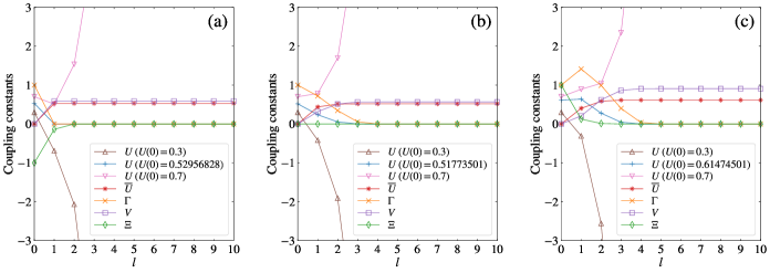
Figure 4: Coupling constants $U(l)$, $\overline{U}(l)$, $\Gamma(l)$, $V(l)$, and $\Xi(l)$ as functions of $l$ for the bare couplings $(\Gamma(0),V(0),\Xi(0))=(1,0,-1)$ in (a), $(1,0,0)$ in (b), and $(1,0,1)$ in (c). In each of the cases, $U(0)=0.3,\overline{U}_{\Gamma(0),\Xi(0)},0.7$. Note that $\overline{U}(l)$, $\Gamma(l)$, $V(l)$, and $\Xi(l)$ do not depend on $U(0)$.

We find that $\overline{U}(l)$ and $V(l)$ converge to finite positive values and $\Gamma(l)$ and $\Xi(l)$ vanish in the limit $l\to\infty$. The coupling constant $U(l)$ asymptotically behaves as

$$U(l)\approx 3^{l}(U(0)-\overline{U}_{\Gamma(0),\Xi(0)})\quad(l\to\infty),$$ (14)

where $\overline{U}_{\Gamma(0),\Xi(0)}:=\lim_{l\to\infty}\overline{U}(l)$ is the limiting value of $\overline{U}(l)$ determined by the bare couplings $\Gamma(0)$ and $\Xi(0)$ [recall that $V(0)=0$]. Figure 4 shows the behavior of $U(l)$ for several values of $U(0)$ including $\overline{U}_{\Gamma(0),\Xi(0)}$. It turns out that the limit of $U(l)$ is

$$U(l)\to\left\{\begin{aligned} &{-\infty},\quad&&U(0)<\overline{U}_{\Gamma(0),\Xi(0)},\\ &0,\quad&&U(0)=\overline{U}_{\Gamma(0),\Xi(0)},\\ &{+\infty},\quad&&U(0)>\overline{U}_{\Gamma(0),\Xi(0)}\end{aligned}\right.\quad(l\to\infty).$$ (15)

This indicates that the fixed points of the present RG transformation are $(U,\Gamma,V,\Xi)=(0,0,V,0),(\pm\infty,0,V,0)$ with $V$ being an arbitrary positive value. Indeed, we can confirm that these points are fixed points by finding that $f_{\Gamma=0,V,\Xi=0}(\alpha_{1},\alpha_{2},z,\beta_{1},\beta_{2})$ is minimized at $\alpha_{1}^{2}=\beta_{1}^{2}=1$ and $\alpha_{2}=z=\beta_{2}=0$ under the constraint (11) and substituting these values into the RG equations (9).

To gain a clearer understanding of the behavior of the coupling constants, we depict the RG flow diagrams in Fig. 5. We see that the coupling constants approach the following values in the limit $l\to\infty$:

$$\lim_{l\to\infty}(U(l),\Gamma(l),V(l),\Xi(l))$$

$$=\left\{\begin{aligned} &\left(-\infty,0,\lim_{l\to\infty}V(l),0\right),\quad&&U(0)<\overline{U}_{\Gamma(0),\Xi(0)},\\ &\left(0,0,\lim_{l\to\infty}V(l),0\right),\quad&&U(0)=\overline{U}_{\Gamma(0),\Xi(0)},\\ &\left(+\infty,0,\lim_{l\to\infty}V(l),0\right),\quad&&U(0)>\overline{U}_{\Gamma(0),\Xi(0)},\end{aligned}\right.$$ (16)

where $\lim_{l\to\infty}V(l)$ is a finite positive value.

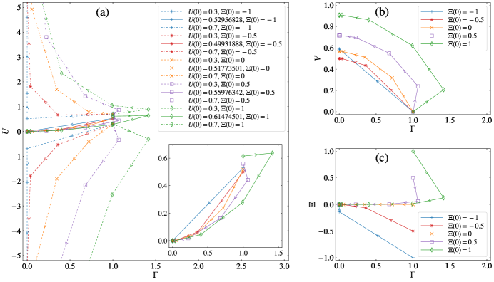
Figure 5: RG flow diagrams of the frustrated Ising ladder in the dimer limit $K\to\infty$. We plot $(\Gamma(l),U(l))$, $(\Gamma(l),V(l))$, and $(\Gamma(l),\Xi(l))$ ($l=0,1,\dots,10$) in (a), (b), and (c), respectively. The bare couplings are set to $\Gamma(0)=1$, $V(0)=0$, $\Xi(0)=0,\pm 0.5,\pm 1$, and $U(0)=0.3,\overline{U}_{\Gamma(0),\Xi(0)},0.7$. Note that $\Gamma(l)$, $V(l)$, and $\Xi(l)$ do not depend on $U(0)$. The inset in (a) is a magnification of $(\Gamma(l),U(l))$ for $U(0)=\overline{U}_{\Gamma(0),\Xi(0)}$. The arrows on each line indicate the direction of the RG flow. It can be seen that $l=10$ is sufficient for convergence of $U(l)$ [$U(0)=\overline{U}_{\Gamma(0),\Xi(0)}$], $\Gamma(l)$, $V(l)$, and $\Xi(l)$.

The fixed points $(U,\Gamma,V,\Xi)=(\pm\infty,0,V,0)$ ($V>0$) are stable (i.e., any coupling constant is irrelevant around these fixed points) and these correspond to the two phases:

• $(U,\Gamma,V,\Xi)=(-\infty,0,V,0)$: symmetric phase

• $(U,\Gamma,V,\Xi)=(+\infty,0,V,0)$: staggered phase

On the other hand, the fixed point $(U,\Gamma,V,\Xi)=(0,0,V,0)$ for each $V>0$ is unstable to variations in $U$. Around this fixed point, $U$ is relevant and the other coupling constants are irrelevant.${}^{\ref{ftn.rsrg_vmarginal}}$ Recalling that the scaling factor of our RG transformation is $b=3$ and $U(l)$ is asymptotically proportional to $3^{l}$ as shown in Eq. (14), we find that the scaling dimension of $U$ around the unstable fixed point $(U,\Gamma,V,\Xi)=(0,0,V,0)$ is $y_{U}=1$. Here, the scaling dimension $y_{U}$ around a fixed point $U=U^{*}$ is defined as $U(l+1)-U^{*}\approx b^{y_{U}}(U(l)-U^{*})$ in the vicinity of $U(l)=U^{*}$ for any scaling factor $b$.

In addition, Eq. (16) shows the bare coupling $U(0)=\overline{U}_{\Gamma(0),\Xi(0)}$ to be the critical point for each $\Gamma(0)$ and $\Xi(0)$, meaning that only the fine-tuned $U(0)=\overline{U}_{\Gamma(0),\Xi(0)}$ flows into the unstable fixed point $(U,\Gamma,V,\Xi)=(0,0,V,0)$ in the sense of RG theory. Other values of the bare coupling $U(0)$ are absorbed into the stable fixed points [namely, $U(0)<\overline{U}_{\Gamma(0),\Xi(0)}$ into the symmetric phase $(U,\Gamma,V,\Xi)=(-\infty,0,V,0)$ and $U(0)>\overline{U}_{\Gamma(0),\Xi(0)}$ into the staggered phase $(U,\Gamma,V,\Xi)=(+\infty,0,V,0)$] under repeated application of the RG transformation.

III.1.4 Phase diagram

We now obtain the phase diagram of the frustrated Ising ladder in the dimer limit. In the following, we denote the bare couplings by $U$, $\Gamma$, and $\Xi$ [not $U(0)$, $\Gamma(0)$, and $\Xi(0)$] for notational simplicity. Although there are three couplings $U$, $\Gamma$, and $\Xi$, it suffices to plot the phase diagram in the $\Xi/U$-$\Gamma/U$ plane because dividing these couplings by $U>0$ does not change the phase [note, as already remarked above, that $\overline{U}_{c\Gamma,c\Xi}=c\overline{U}_{\Gamma,\Xi}$ for any $c>0$ and thus $\lim_{l\to\infty}U(l)$ is unchanged under multiplication of every bare coupling by $c$]. We can draw the phase diagram by marking the critical points $(\Gamma/U,\Xi/U)=(\Gamma/\overline{U}_{\Gamma,\Xi},\Xi/\overline{U}_{\Gamma,\Xi})$ for a number of sets of $\Gamma$ and $\Xi$. The resulting phase diagram is shown in Fig. 6.

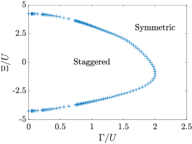
Figure 6: Phase diagram of the frustrated Ising ladder in the dimer limit $K\to\infty$ predicted by the real-space RG method. The first-order transition points (blue plus signs) indicate that adding $XX$ catalysts (stoquastic or nonstoquastic) does not remove the first-order transition.

We can deduce from scaling theory Nishimori and Ortiz (2011), which is closely related to RG theory, that the phase boundary shown in Fig. 6 is of first order. The fact that the scaling dimension of the longitudinal field on the bottom row $y_{U}$ is equal to the spatial dimensionality of the system $d=1$ indicates that the phase transition is of first order, because the correlation function on the bottom row at the critical point does not decay:

$$G_{\mathrm{b}i,\mathrm{b}j}:=\braket{\hat{Z}_{\mathrm{b},i}\hat{Z}_{\mathrm{b},j}}_{U=\overline{U}_{\Gamma,\Xi}}\sim\lvert i-j\rvert^{-2(d-y_{U})}=1,$$ (17)

where $\braket{\cdots}_{U=\overline{U}_{\Gamma,\Xi}}$ denotes the expectation value at the critical point $U=\overline{U}_{\Gamma,\Xi}$ and the approximation is a consequence of scaling theory Nishimori and Ortiz (2011). This behavior of the correlation function leads to the value of the anomalous dimension $\eta$, one of the critical exponents defined by $G_{\mathrm{b}i,\mathrm{b}j}\sim\lvert i-j\rvert^{2-d-\eta}$:

$$\eta=2+d-2y_{U}=2-d=1.$$ (18)

Recall that in general the scaling law for a quantum system is $G_{\mathrm{b}i,\mathrm{b}j}\sim\lvert i-j\rvert^{-2(d+z-y_{U})}$ with $z$ being the dynamic critical exponent Sachdev (2011) (which should not be confused with the variational parameter $z$) instead of Eq. (17). However, we find that $z=0$ for the present system, because under a sufficiently large number of RG transformations the system becomes (almost) classical, by elimination of the transverse field $\Gamma$ and the $XX$ interaction $\Xi$.

Consequently, Fig. 6 demonstrates that there is a first-order phase boundary that completely separates the staggered phase from the symmetric phase on the $\Xi/U$-$\Gamma/U$ plane. In other words, the first-order phase transition encountered during quantum annealing cannot be removed by stoquastic or nonstoquastic $XX$ catalysts.

Note that whether the bare Hamiltonian (1) is nonstoquastic depends not only on $\Xi$ ($=\Xi_{\mathrm{t}\mathrm{t}}$) but also on $\Gamma$ ($=\Gamma_{\mathrm{t}}$), $\Gamma_{\mathrm{b}}$, $\Xi_{\mathrm{b}\mathrm{b}}$, and $\Xi_{\mathrm{t}\mathrm{b}}$ [recall that the Hamiltonian is nonstoquastic if the fields and interactions satisfy Eq. (3), whose third condition $\lvert U/2\rvert,\lvert\Xi_{\mathrm{t}\mathrm{b}}\rvert<K$ holds in the dimer limit $K\gg U,\Gamma_{a},\Xi_{aa^{\prime}}$]. For example, consider the case of $\mathop{\mathrm{sgn}}\Gamma_{\mathrm{b}}=\mathop{\mathrm{sgn}}\Gamma$ and $\mathop{\mathrm{sgn}}\Xi_{\mathrm{b}\mathrm{b}},\mathop{\mathrm{sgn}}\Xi_{\mathrm{t}\mathrm{b}}\in\{0,\mathop{\mathrm{sgn}}\Xi\}$, where the sign function is defined as $\mathop{\mathrm{sgn}}x=x/\lvert x\rvert$ for $x\not=0$ and $\mathop{\mathrm{sgn}}x=0$ for $x=0$. Then, the Hamiltonian is stoquastic if $\Gamma=0\vee\Xi\geq 0$ and nonstoquastic if $\Gamma>0\wedge\Xi<0$. Stoquasticity for $\Gamma=0\wedge\Xi<0$ follows from the curing transformation that flips the signs of $\Xi_{\mathrm{t}\mathrm{t}}$, $\Xi_{\mathrm{b}\mathrm{b}}$, and $\Xi_{\mathrm{t}\mathrm{b}}$, as pointed out in Sec. II.1. The existence of this transformation indicates that the critical points on $\Gamma=0$, $\overline{U}_{\Gamma=0,\Xi}$, are invariant under a change of the sign of $\Xi$.

It is noteworthy that the transition point derived from our real-space RG method in the absence of $XX$ interactions, $\Gamma/U=\Gamma/\overline{U}_{\Gamma,\Xi=0}=1.9314900$, is not far from that obtained by numerical diagonalization of the quantum dimer model (whose Hamiltonian is given by Eq. (7) with $\Xi_{\mathrm{t}\mathrm{t}}=0$), $\Gamma/U\approx 1/0.6=1.66\dotsm$ Laumann et al. (2012), in spite of the fact that our RG analysis is not an exact method.

III.2 Small frustration limit of the Ising chain

In this section we step back from the full Ising ladder and analyze the phase transition in the limit of small frustration $U\gg K,\Gamma_{a},\Xi_{aa^{\prime}}$ at zero temperature. Since the bottom spins are fixed to down in this limit, we obtain an antiferromagnetic Ising chain with a transverse field and $XX$ interactions as an effective model:

$$\hat{H}_{\text{chain}}=\sum_{i=1}^{L}(K\hat{Z}_{\mathrm{t},i}\hat{Z}_{\mathrm{t},i+1}-\Gamma_{\mathrm{t}}\hat{X}_{\mathrm{t},i}-\Xi_{\mathrm{t}\mathrm{t}}\hat{X}_{\mathrm{t},i}\hat{X}_{\mathrm{t},i+1}).$$ (19)

Our purpose in this section is to reveal how the $XX$ interactions affect the second-order transition that appears in the case of no $XX$ interaction and large $U$ (see Fig. 2 or Ref. Laumann et al. (2012)). Readers who are interested only in the effects of the $XX$ interactions on the first-order transition can proceed to the next section on the DMRG calculations.

Similar analyses were conducted by Langari Langari (1998, 2004). He carried out the real-space RG analysis of the $XXZ$ chain in a magnetic field Langari (1998), whose Hamiltonian is equivalent to Eq. (19) with $\sum_{i}K\hat{Y}_{\mathrm{t},i},\hat{Y}_{\mathrm{t},i+1}$ added, and derived the zero-temperature phase diagram. In addition, he obtained the zero-temperature phase diagram of the model given by the Hamiltonian (19) for $\Xi_{\mathrm{t}\mathrm{t}}\leq 0$ using the real-space RG method Langari (2004).

To compare the effects of ferromagnetic and antiferromagnetic $XX$ interactions, we perform the real-space RG analysis for positive and negative $\Xi_{\mathrm{t}\mathrm{t}}$. Instead of the Hamiltonian (19), we consider the ferromagnetic Ising chain with a transverse field and $XX$ interactions,

$$\hat{H}=\sum_{i=1}^{L}(-K\hat{Z}_{i}\hat{Z}_{i+1}-\Gamma\hat{X}_{i}-\Xi\hat{X}_{i}\hat{X}_{i+1}),$$ (20)

which is obtained by the gauge transformation $(\hat{X}_{i},\hat{Y}_{i},\hat{Z}_{i})\mapsto(\hat{X}_{i},-\hat{Y}_{i},-\hat{Z}_{i})$ for every odd $i$ (we omitted the subscript $\mathrm{t}$ in $\Gamma_{\mathrm{t}}$, $\Xi_{\mathrm{t}\mathrm{t}}$, and the Pauli operators for notational simplicity).

The real-space RG analysis of the model (20) proceeds in the standard manner Nishimori and Ortiz (2011), which is detailed in Appendix C. We first separate the Hamiltonian into intrablock and interblock Hamiltonians after partitioning the chain every two sites, which is valid when $\Xi$ is not a negative large value (if $\Xi<0$ and $\lvert\Xi\rvert$ is large, block partitioning every odd number of sites will be needed to retain the antiferromagnetic order in the $x$ direction). Then, we diagonalize the intrablock Hamiltonian and project the Hilbert space onto the two-dimensional low-energy subspace in each block. Our real-space RG transformation is slightly different from that in Ref. Langari (2004), in the sense that the intrablock Hamiltonian in our transformation includes the magnetic field only at the left site in each block while that in Ref. Langari (2004) includes the fields at both sites. An advantage of our scheme is that the critical point $\Gamma=\Gamma_{\mathrm{c}}$ and the critical exponent $\nu$ for $\Xi=0$ coincide with the exact results $\Gamma_{\mathrm{c}}=K$ and $\nu=1$, where $\nu$ is defined by the correlation length $L_{\mathrm{corr}}\sim\lvert\Gamma-\Gamma_{\mathrm{c}}\rvert^{-\nu}$ near the critical point Nishimori and Ortiz (2011).

We focus on the case where the magnitude of the $XX$ interactions is not large, or more precisely $\lvert\Xi\rvert<\sqrt{K^{2}+\Gamma^{2}}$. Since the overall energy scale is unimportant at zero temperature, we consider the ratios of the coupling constants $\gamma=\Gamma/K$ and $\xi=\Xi/K$. As derived in Appendix C, we find the RG equations

$$\gamma(l+1)=\gamma(l)^{2}+\frac{\xi(l)(1+2\gamma(l)^{2})}{\sqrt{1+\gamma(l)^{2}}},\quad\xi(l+1)=0$$ (21)

for $l\geq 0$, where $\gamma(l)$ and $\xi(l)$ denote the coupling constants after $l$ RG steps.

It turns out that there are three fixed points $(\gamma,\xi)=(0,0),(1,0),(\infty,0)$. The two fixed points $(\gamma,\xi)=(0,0),(\infty,0)$ are stable and correspond to the staggered and symmetric phases in the original Ising ladder (1), respectively. The other fixed point $(\gamma,\xi)=(1,0)$ is unstable under deviations in $\gamma$. Around this fixed point, $\gamma$ has the scaling dimension $y_{\gamma}=1$ since $\gamma(l+1)-1=\gamma(l)^{2}-1\approx 2(\gamma(l)-1)$ for $l\geq 1$ and the present scaling factor is two. Thus, we have the critical exponent $\nu=1/y_{\gamma}=1$ Nishimori and Ortiz (2011).

Equation (21) indicates that the $XX$ interaction is irrelevant in the limit $U\to\infty$ unless the bare magnitude $\lvert\Xi\rvert$ is large. This consequence is consistent with the result in Ref. Langari (2004), which predicts that the antiferromagnetic $XX$ interaction gradually disappears when its bare magnitude is not large. It is also known for the model (19) with the antiferromagnetic $YY$ interactions of the magnitude $K$ that $\Xi$ is irrelevant for $\lvert\Xi/K\rvert\leq 1$ regardless of the sign of $\Xi$ Langari (1998).

The critical points are determined by the equation

$$\gamma^{2}+\frac{\xi(1+2\gamma^{2})}{\sqrt{1+\gamma^{2}}}=1\iff\xi=\frac{(1-\gamma^{2})\sqrt{1+\gamma^{2}}}{1+2\gamma^{2}}$$ (22)

for the bare couplings $\gamma$ and $\xi$. Note that all the critical points but $(\gamma,\xi)=(0,1)$ are inside the region $\lvert\xi\rvert<\sqrt{1+\gamma^{2}}$, in which our analysis can be applied. Since the RG equations (21) imply that the antiferromagnetic Ising chain with the transverse field and the $XX$ interactions belongs to the same universality class as the transverse-field Ising chain, there will be second-order transitions at the critical points (22). We show the phase diagram in Fig. 7, which indicates that the $\pm XX$-type catalysts do not eliminate the second-order phase transition encountered during quantum annealing. The phase diagram is in qualitative agreement with the diagrams obtained by Langari Langari (1998, 2004), though the model in Ref. Langari (2004) covers only the case of the antiferromagnetic $XX$ interactions and that in Ref. Langari (1998) includes the $YY$ interactions that have the same sign and magnitude as the $ZZ$ interactions.

Figure 7: Phase diagram of the Ising ladder in the limit $U\to\infty$ (the Ising chain) predicted by the real-space RG method. The blue line indicates second-order transition points.

IV DMRG calculation

We next employ the DMRG method White (1992, 1993); Schollwöck (2005); Hallberg (2006) to obtain the phase diagram with a moderate coupling magnitude of $K/U$ in Sec. IV.1, which supplements the real-space RG analysis. In addition, we compute the energy gap of the finite-size system with a nonstoquastic $XX$ catalyst in Sec. IV.2.

IV.1 Phase diagram

We perform the DMRG calculations for the frustrated Ising ladder with the transverse fields $\Gamma_{\mathrm{t}}=\Gamma_{\mathrm{b}}=\Gamma$ and the $XX$ interactions $\Xi_{\mathrm{t}\mathrm{t}}=\Xi$ and $\Xi_{\mathrm{b}\mathrm{b}}=\Xi_{\mathrm{t}\mathrm{b}}=0$ in Eq. (1).

To avoid trapping of the calculations in one of energy local minima, we start with several sweeps by taking not only the ground state but also the first excited state as the target states in the finite DMRG procedure, followed by the single target DMRG procedure to obtain the convergence of the ground-state energy. The truncation number $m$ of the density-matrix eigenvalues in the DMRG calculations is set as large as $m=200$ to achieve a maximal truncation error less than $10^{-12}$.

We first show the ground-state phase diagram for $K/U=5$ and $L=20$ in Fig. 8. Since the third condition of Eq. (3) is satisfied, the Hamiltonian is stoquastic for $\Gamma=0\vee\Xi\geq 0$ and nonstoquastic for $\Gamma>0\wedge\Xi<0$. It is significant that the phase diagram obtained by the DMRG method has a similar shape to that for $K\to\infty$ in the thermodynamic limit $L\to\infty$ predicted by the real-space RG method (see Fig. 6 for the latter diagram). As explained below, the phase boundary between the staggered phase and the symmetric phase in Fig. 8 is characterized by first-order transitions.

Figure 8: Ground-state phase diagram of the frustrated Ising ladder obtained by the DMRG calculations with $K/U=5$ and $L=20$ under periodic boundary conditions. We set $\Gamma_{\mathrm{t}}=\Gamma_{\mathrm{b}}=\Gamma$, $\Xi_{\mathrm{t}\mathrm{t}}=\Xi$, and $\Xi_{\mathrm{b}\mathrm{b}}=\Xi_{\mathrm{t}\mathrm{b}}=0$ in Eq. (1). The staggered and symmetric phases are separated by a line of first-order transitions.

In order to determine the phase boundary in Fig. 8, we calculate the staggered order parameter for spins on the top row defined as

$$S=\frac{1}{L^{2}}\sum_{i=1}^{L}\sum_{j=1}^{L}(-1)^{i-j}\braket{\hat{Z}_{\mathrm{t},i}\hat{Z}_{\mathrm{t},j}},$$ (23)

where $\braket{\cdots}$ denotes an average over the ground-state wave function. Figure 9(a) shows the results for $K/U=5$ and $L=20$ as a function of $\Gamma/U$ with several representative values of $\Xi/U$. When $\Xi/U=-0.4$, the staggered order parameter $S$ remains approximately $1$ for $\Gamma/U$ up to $\sim 2.2$, indicating that the ground state is in the staggered phase, and then suddenly decreases to almost zero ($S\approx 0.08$) as $\Gamma/U$ increases further, which corresponds to a first-order transition to the symmetric phase. A similar behavior continues until $\Xi/U\approx-2.65$ with varying $\Gamma/U$ as shown in Fig. 9(a), e.g., for $\Xi/U=-2.6$, where the first-order transition occurs at $\Gamma/U\approx 1.1$. On the other hand, when $\Xi/U=-3.0$, the staggered order parameter $S$ gradually increases from $S\approx 0.08$ with $\Gamma/U$, implying that the ground state remains in the symmetric phase. Indeed, as shown in Fig. 9(b), the first-order transition from the staggered phase to the symmetric phase occurs at $\Xi/U\approx\pm 2.65$ when $\Gamma=0$.

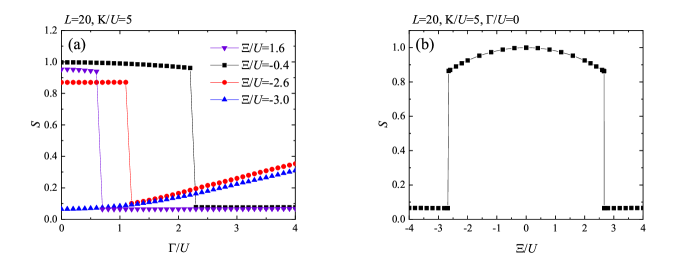
Figure 9: Staggered order parameter on the top row $S$ (a) as a function of $\Gamma/U$ with several values of $\Xi/U$ and (b) as a function of $\Xi/U$ with $\Gamma=0$. The results are obtained by the DMRG method for $K/U=5$ and $L=20$ under periodic boundary conditions.

To support these results, we calculate the first derivatives of the ground-state energy $E_{0}=\braket{\hat{H}}$ with respect to $\Gamma$ and $\Xi$ since a first-order transition is characterized by a point where $\partial E_{0}/\partial\Gamma$ or $\partial E_{0}/\partial\Xi$ is discontinuous. According to the Hellmann-Feynman theorem Feynman (1939), the first derivatives of the ground-state energy $E_{0}$ with respect to $\Gamma$ and $\Xi$ are calculated as

$$\frac{\partial E_{0}}{\partial\Gamma} =-\sum_{i=1}^{L}\braket{\hat{X}_{\mathrm{t},i}+\hat{X}_{\mathrm{b},i}},$$ (24a)

$$\frac{\partial E_{0}}{\partial\Xi} =-\sum_{i=1}^{L}\braket{\hat{X}_{\mathrm{t},i}\hat{X}_{\mathrm{t},i+1}}.$$ (24b)

As shown in Fig. 10, the first derivatives of the ground-state energy $E_{0}$ with respect to $\Gamma$ and $\Xi$ exhibit discontinuities exactly at the points where the staggered order parameter $S$ changes abruptly in Fig. 9, confirming the first-order nature of the transition.

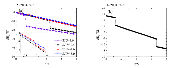
Figure 10: First derivatives of the ground-state energy $E_{0}$ (a) with respect to $\Gamma$ for several values of $\Xi/U$ and (b) with respect to $\Xi$ for $\Gamma=0$. The results are obtained by the DMRG method for $K/U=5$ and $L=20$ under periodic boundary conditions. The inset in (a) is a magnification around $\Gamma/U=1$.

IV.2 Energy gap

We next obtain the energy gap between the ground state and the first excited state of the finite-size system with a nonstoquastic $XX$ catalyst using the DMRG method. We adopt the multi-target DMRG procedure with the ground state as well as the two lowest excited states as the target states, taking the truncation number $m$ as large as $2{,}000$. We show in Fig. 11 the finite-size scaling of the minimum gap $\Delta(L)$ through the first-order transition driven by varying $\Gamma/U$ at $K/U=5$ for $\Xi/U=0,-1,-2$. We find that the gap $\Delta(L)$ decreases exponentially with $L$, i.e., $\ln\Delta(L)\sim-\alpha L$, for all three values of $\Xi/U$ (for $\Xi/U=0$ and $L\leq 12$, we reproduce the previously reported results in Ref. Laumann et al. (2012)). It is noteworthy that the absolute value of the slope, $\alpha$, in $\ln\Delta(L)$ tends to be smaller in the presence of negative $\Xi$. From the point of view of quantum annealing and optimization this implies a quantitative, if not qualitative, improvement by the nonstoquastic $XX$ catalyst, since a larger gap implies a faster time-to-solution by the adiabatic theorem Morita and Nishimori (2008); Albash and Lidar (2018).

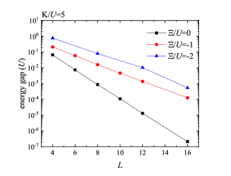
Figure 11: The finite-size scaling of the minimum gap through the first-order transition driven by varying $\Gamma/U$ at a fixed value of $K/U=5$. The results are obtained by the DMRG method for three values of $\Xi/U$ under periodic boundary conditions.

We now discuss why the nonstoquastic $XX$ catalyst reduces the decay rate $\alpha$ of the minimum gap $\Delta(L)$. Consider the sum of the terms with the coefficients $U$, $\Gamma$, and $\Xi$ in the Hamiltonian $\hat{H}$ as a perturbation. It may be expected that the ground state and the first excited state at the transition are superpositions of columnar and staggered configurations and $\ln\Delta(L)$ is roughly proportional to $L\ln(\Gamma/K)$, because all the bottom spins need to be flipped by the bottom transverse field $\Gamma_{\mathrm{b}}=\Gamma$ to move from the symmetric phase to the staggered phase (note that the present $XX$ interactions $\Xi$ are applied only along the top row and cannot flip the bottom spins). Indeed, $\log_{10}(1.85/5)=-0.43$ and $\log_{10}(2.85/5)=-0.24$ are close to the slopes of the lines for $\Xi/U=0,-2$ in Fig. 11, respectively, where $\Gamma/U=1.85$ is the transition point for $\Xi/U=0$ and $\Gamma/U=2.85$ is for $\Xi/U=-2$ when $K/U=5$ (see Fig. 8). This is consistent with the fact that the decay rate $\alpha$ is proportional to $\ln(K/\Gamma)$ when $K/U$ is varied in the absence of the $XX$ catalyst Laumann et al. (2012). Our argument suggests that the nonstoquastic $XX$ catalyst on the top row with an appropriate magnitude $\Xi$ increases the transverse field $\Gamma$ at the transition and reduces the exponential decay rate of the gap in the present system. Although we have not carried out a numerical calculation of the gap of the model with the stoquastic $XX$ catalyst due to the associated heavy computational cost, it is implied that the decay rate $\alpha$ of the minimum gap $\Delta(L)$ becomes larger for $\Xi>0$ (as well as for $\Xi/U\lesssim-2.5$) than for $\Xi=0$, because $\Gamma/U$ at the transition is smaller in the former case, as shown in Fig. 8.

Similar arguments were presented for a geometrically local Ising model on two connected rings Albash (2019). There it was shown by numerical diagonalization that the nonstoquastic $XX$ catalyst makes the minimum gap larger than in the case without the $XX$ catalyst and in the case with the stoquastic $XX$ catalyst. It was argued that one of the possible reasons for the softening of the avoided level crossing with the nonstoquastic catalyst is that the driver with the nonstoquastic $XX$ catalyst causes the level crossing earlier in quantum annealing (which means a larger transverse field) than with the stoquastic $XX$ catalyst, which is a consequence of perturbation theory.

V Summary and Conclusions

We have studied the effects of stoquastic and nonstoquastic catalysts, implemented via ferromagnetic and antiferromagnetic $XX$ interactions, in the setting of the frustrated Ising ladder. This model – without the $XX$ interactions – is known to have a first-order phase transition with an exponentially decaying energy gap, which is characterized by a change in the topology of dimer configurations in the limit of strong frustration $K\to\infty$ Laumann et al. (2012). We have formulated a real-space RG transformation such that the symmetry of the problem is preserved and used it to obtain the phase diagram in the presence of $XX$ interactions of both signs, stoquastic and nonstoquastic. The result shows that the first-order transition persists in the presence of $XX$ interactions of moderate magnitude. The transition point obtained by the real-space RG method in the case without $XX$ interactions is close to the value obtained by numerical diagonalization Laumann et al. (2012). This is surprising, given that the real-space RG approach involves a number of uncontrolled approximations. In addition, we applied the real-space RG method to the case with small frustration and found that the second-order transition persists under the influence of $XX$ interactions of moderate magnitude.

We next performed extensive numerical computations by the DMRG method for a large but finite value of $K$ in order to directly study the behavior of various physical quantities. The results for the order parameter and derivatives of the ground-state energy clearly indicate the existence of first-order phase transitions in the presence of stoquastic or nonstoquastic $XX$ interactions, which is consistent with the conclusion from the real-space RG study. The structure of the phase diagram qualitatively and even semi-quantitatively resembles the one obtained by the real-space RG analysis. Our DMRG results furthermore confirm that the energy gap decays exponentially as a function of system size at the first-order transition points, both with or without $XX$ interactions on the top row of the ladder. However, the nonstoquastic $XX$ catalyst reduces the decay rate of the gap, as we showed numerically. We pointed out that this softening of the exponential decay of the gap may be due to an increase of the transverse field at the transition in the presence of a nonstoquastic catalyst.

A first-order phase transition is a sudden change of the system state between very different phases, e.g., between water and ice, and is unlikely to be induced or reduced by a series of gradual local changes. In the case of spin systems, the latter gradual change is exemplified by the introduction of $XX$ interactions, which change the state of the system in the computational basis by flipping only pairs of spins simultaneously. Nevertheless, there exist examples in which nonstoquastic $XX$ interactions change the order of a phase transition from first to second Seki and Nishimori (2012); Seoane and Nishimori (2012); Seki and Nishimori (2015); Nishimori and Takada (2017); Albash (2019); Takada et al. (2020), meaning a drastic reduction of the “strength” of the phase transition by nonstoquastic $XX$ interactions, although counterexamples abound Crosson et al. (2020).

The first-order transition in the problem of the frustrated Ising ladder without $XX$ interactions belongs to a more stable class in the sense that the two phases are separated by different topological structures in the limit of strong frustration. These topological structures are generated by the columnar and staggered configurations, which have magnetizations with opposite signs on the bottom row of the ladder. In the presence of frustration of infinite magnitude, the addition of any local operators of finite magnitude does not allow transitions between the topologically distinct states. It is therefore expected that the first-order transition is stable against the introduction of the $XX$ interactions of either sign.

From the perspective of quantum annealing, the persistence of the first-order transition means that the computational complexity of the problem, exponential in the system size, remains intact under the introduction of stoquastic or nonstoquastic $XX$ catalysts as long as the system evolves under adiabatic unitary dynamics. It is an important and interesting open question to study whether any of these conclusions are modified under nonunitary (open-system) dynamics or diabatic evolution, both of which take place in real quantum devices Crosson and Lidar (2021).

Appendix A Energy gap of the model without $XX$ terms

This appendix displays additional data to supplement the phase diagram of the Ising ladder without $XX$ terms in Fig. 2. As mentioned in Sec. II.2, it appears that the minimum gap point (namely, the location at which the energy gap between the ground state and the first excited state is minimized for a fixed $K/U$) has a discontinuity at $K/U\approx 1.5$ between $\Gamma/U\approx 1.5$ and $1.9$. To examine whether this phenomenon is a finite-size effect, we plot the minimum gap points for $L=4,6,8,10$ in Fig. 12. We find near convergence already for $L=10$, which suggests that the discontinuity of the minimum gap point location is not a finite size effect.

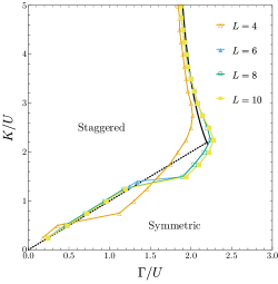
Figure 12: Locations of the minimum energy gap of the Ising ladder with uniform transverse field $\Gamma$ and no $XX$ terms for several system sizes $L$, at fixed values of $K/U$. The first- and second-order phase boundaries predicted by perturbation theory are indicated by black solid and dashed lines, respectively.

An explanation is provided in Fig. 13, which shows the energy gap $\Delta E$ as a function of $\Gamma/U$ for $L=10$ and $K/U=1.25,1.49,1.5,1.75$. It turns out that the energy gap for $K/U\approx 1.5$ takes a “double-well” form, which is the origin of the discontinuity of the minimum gap point. The energy gap $\Delta E$ is minimized in the left “well” for $K/U\lesssim 1.5$, while $\Delta E$ is minimized in the right “well” for $K/U\gtrsim 1.5$. We leave a detailed understanding of this phenomenon as a future topic of research.

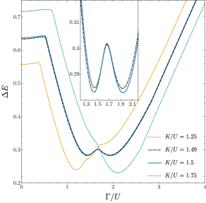
Figure 13: Energy gap $\Delta E$ as a function of $\Gamma/U$ for $L=10$ at different values of $K/U$. The inset is a magnification of the lines for $K/U=1.49,1.5$, which shows that the global minimum of $\Delta E$ moves from the left “well” to the right “well” as $K/U$ changes.

Appendix B Derivation of RG equations in the limit of large frustration

We derive the RG equations of the frustrated Ising ladder in the limit of large frustration (i.e., the dimer limit), which were used in Sec. III.1. Appendix B.1 gives a review of basic properties of the model. In Appendix B.2, we define a Hamiltonian that appears in the RG analysis. In Appendices B.3–B.7, we explain the way to construct the real-space RG transformation including the variational ansatz in detail and write down the RG equations. We also calculate the renormalized couplings and show their behavior.

B.1 Preliminary analysis

To prepare for the real-space RG analysis, we demonstrate why the columnar and staggered configurations are the low-energy states of the frustrated Ising ladder (1) in the dimer limit $K\to\infty$ and derive the number of low-energy states, as indicated in Ref. Laumann et al. (2012).

Since the overall energy scale does not change the statistical properties in the zero-temperature limit, we consider the dimensionless Hamiltonian $\hat{h}=\hat{H}/K$:

$$\hat{h} =\sum_{i=1}^{L}\Bigl{(}\hat{Z}_{\mathrm{t},i}\hat{Z}_{\mathrm{t},i+1}-\hat{Z}_{\mathrm{b},i}\hat{Z}_{\mathrm{b},i+1}-\hat{Z}_{\mathrm{t},i}\hat{Z}_{\mathrm{b},i}-\hat{Z}_{\mathrm{t},i}$$

$$\hphantom{{}=\sum\Bigl{(}}+\frac{u}{2}\hat{Z}_{\mathrm{b},i}-(\gamma_{\mathrm{t}}\hat{X}_{\mathrm{t},i}+\gamma_{\mathrm{b}}\hat{X}_{\mathrm{b},i})-(\xi_{\mathrm{t}\mathrm{t}}\hat{X}_{\mathrm{t},i}\hat{X}_{\mathrm{t},i+1}+\xi_{\mathrm{b}\mathrm{b}}\hat{X}_{\mathrm{b},i}\hat{X}_{\mathrm{b},i+1}+\xi_{\mathrm{t}\mathrm{b}}\hat{X}_{\mathrm{t},i}\hat{X}_{\mathrm{b},i})\Bigr{)},$$ (25)

where $u=U/K$, $\gamma_{a}=\Gamma_{a}/K$, and $\xi_{aa^{\prime}}=\Xi_{aa^{\prime}}/K$ are sufficiently small dimensionless parameters. We assume that $u$, $\gamma_{a}$, and $\xi_{aa^{\prime}}$ are of the same order $\delta\ll 1$. We separate the Hamiltonian $\hat{h}$ into $\hat{h}^{(0)}=\mathcal{O}(\delta^{0})$ and $\hat{h}^{(1)}=\mathcal{O}(\delta^{1})$:

$$\hat{h} =\hat{h}^{(0)}+\hat{h}^{(1)},$$ (26a)

$$\hat{h}^{(0)} =\sum_{i=1}^{L}(\hat{Z}_{\mathrm{t},i}\hat{Z}_{\mathrm{t},i+1}-\hat{Z}_{\mathrm{b},i}\hat{Z}_{\mathrm{b},i+1}-\hat{Z}_{\mathrm{t},i}\hat{Z}_{\mathrm{b},i}-\hat{Z}_{\mathrm{t},i}),$$ (26b)

$$\hat{h}^{(1)} =\sum_{i=1}^{L}\left(\frac{u}{2}\hat{Z}_{\mathrm{b},i}-(\gamma_{\mathrm{t}}\hat{X}_{\mathrm{t},i}+\gamma_{\mathrm{b}}\hat{X}_{\mathrm{b},i})-(\xi_{\mathrm{t}\mathrm{t}}\hat{X}_{\mathrm{t},i}\hat{X}_{\mathrm{t},i+1}+\xi_{\mathrm{b}\mathrm{b}}\hat{X}_{\mathrm{b},i}\hat{X}_{\mathrm{b},i+1}+\xi_{\mathrm{t}\mathrm{b}}\hat{X}_{\mathrm{t},i}\hat{X}_{\mathrm{b},i})\right).$$ (26c)

Using translational invariance yields $\sum_{i}\hat{Z}_{\mathrm{t},i}=\sum_{i}(\hat{Z}_{\mathrm{t},i}+\hat{Z}_{\mathrm{t},i+1})/2$ and $\sum_{i}\hat{Z}_{\mathrm{t},i}\hat{Z}_{\mathrm{b},i}=\sum_{i}(\hat{Z}_{\mathrm{t},i}\hat{Z}_{\mathrm{b},i}+\hat{Z}_{\mathrm{t},i+1}\hat{Z}_{\mathrm{b},i+1})/2$. We can thus rewrite the zeroth-order Hamiltonian $\hat{h}^{(0)}$ as

$$\hat{h}^{(0)}=\sum_{i=1}^{L}\left(\hat{Z}_{\mathrm{t},i}\hat{Z}_{\mathrm{t},i+1}-\hat{Z}_{\mathrm{b},i}\hat{Z}_{\mathrm{b},i+1}-\hat{Z}_{\mathrm{t},i}\frac{1+\hat{Z}_{\mathrm{b},i}}{2}-\hat{Z}_{\mathrm{t},i+1}\frac{1+\hat{Z}_{\mathrm{b},i+1}}{2}\right).$$ (27)

Next, let us rewrite the same Hamiltonian as a linear combination of projectors:

$$\hat{h}^{(0)} =\sum_{i=1}^{L}\Biggl{(}{}-2\Ket{\begin{gathered}\uparrow\uparrow\\ \uparrow\uparrow\end{gathered}}\Bra{\begin{gathered}\uparrow\uparrow\\ \uparrow\uparrow\end{gathered}}-2\Ket{\begin{gathered}\downarrow\uparrow\\ \uparrow\uparrow\end{gathered}}\Bra{\begin{gathered}\downarrow\uparrow\\ \uparrow\uparrow\end{gathered}}-2\Ket{\begin{gathered}\uparrow\downarrow\\ \uparrow\uparrow\end{gathered}}\Bra{\begin{gathered}\uparrow\downarrow\\ \uparrow\uparrow\end{gathered}}+2\Ket{\begin{gathered}\downarrow\downarrow\\ \uparrow\uparrow\end{gathered}}\Bra{\begin{gathered}\downarrow\downarrow\\ \uparrow\uparrow\end{gathered}}$$ (44)

$$\hphantom{{}=\sum\Biggl{(}}+0\Ket{\begin{gathered}\uparrow\uparrow\\ \downarrow\downarrow\end{gathered}}\Bra{\begin{gathered}\uparrow\uparrow\\ \downarrow\downarrow\end{gathered}}-2\Ket{\begin{gathered}\downarrow\uparrow\\ \downarrow\downarrow\end{gathered}}\Bra{\begin{gathered}\downarrow\uparrow\\ \downarrow\downarrow\end{gathered}}-2\Ket{\begin{gathered}\uparrow\downarrow\\ \downarrow\downarrow\end{gathered}}\Bra{\begin{gathered}\uparrow\downarrow\\ \downarrow\downarrow\end{gathered}}+0\Ket{\begin{gathered}\downarrow\downarrow\\ \downarrow\downarrow\end{gathered}}\Bra{\begin{gathered}\downarrow\downarrow\\ \downarrow\downarrow\end{gathered}}$$ (61)

$$\hphantom{{}=\sum\Biggl{(}}+1\Ket{\begin{gathered}\uparrow\uparrow\\ \downarrow\uparrow\end{gathered}}\Bra{\begin{gathered}\uparrow\uparrow\\ \downarrow\uparrow\end{gathered}}-1\Ket{\begin{gathered}\downarrow\uparrow\\ \downarrow\uparrow\end{gathered}}\Bra{\begin{gathered}\downarrow\uparrow\\ \downarrow\uparrow\end{gathered}}+1\Ket{\begin{gathered}\uparrow\downarrow\\ \downarrow\uparrow\end{gathered}}\Bra{\begin{gathered}\uparrow\downarrow\\ \downarrow\uparrow\end{gathered}}+3\Ket{\begin{gathered}\downarrow\downarrow\\ \downarrow\uparrow\end{gathered}}\Bra{\begin{gathered}\downarrow\downarrow\\ \downarrow\uparrow\end{gathered}}$$ (78)

$$\hphantom{{}=\sum\Biggl{(}}+1\Ket{\begin{gathered}\uparrow\uparrow\\ \uparrow\downarrow\end{gathered}}\Bra{\begin{gathered}\uparrow\uparrow\\ \uparrow\downarrow\end{gathered}}+1\Ket{\begin{gathered}\downarrow\uparrow\\ \uparrow\downarrow\end{gathered}}\Bra{\begin{gathered}\downarrow\uparrow\\ \uparrow\downarrow\end{gathered}}-1\Ket{\begin{gathered}\uparrow\downarrow\\ \uparrow\downarrow\end{gathered}}\Bra{\begin{gathered}\uparrow\downarrow\\ \uparrow\downarrow\end{gathered}}+3\Ket{\begin{gathered}\downarrow\downarrow\\ \uparrow\downarrow\end{gathered}}\Bra{\begin{gathered}\downarrow\downarrow\\ \uparrow\downarrow\end{gathered}}\Biggr{)}_{i,i+1}.$$ (95)

Here, each state vector containing an array of arrows means a product state and the positions in the array correspond to those in the ladder:

$$\Ket{\begin{gathered}\sigma_{\mathrm{t},i}\\ \sigma_{\mathrm{b},i}\end{gathered}\begin{gathered}\sigma_{\mathrm{t},i+1}\\ \sigma_{\mathrm{b},i+1}\end{gathered}}_{i,i+1}:=\ket{\sigma_{\mathrm{t},i}}_{\mathrm{t},i}\ket{\sigma_{\mathrm{b},i}}_{\mathrm{b},i}\ket{\sigma_{\mathrm{t},i+1}}_{\mathrm{t},i+1}\ket{\sigma_{\mathrm{b},i+1}}_{\mathrm{b},i+1}\quad(\sigma_{a,j}=\uparrow,\downarrow).$$ (96)

We denoted the normalized eigenstates of $\hat{Z}_{a,i}$ with the eigenvalues $+1$ and $-1$ by $\ket{\uparrow}_{a,i}$ and $\ket{\downarrow}_{a,i}$, respectively.

Since a constant energy difference is unimportant, we add $2\hat{I}$ to $\hat{h}^{(0)}$, where $\hat{I}$ is the identity operator, and redefine $\hat{h}^{(0)}+2\hat{I}$ as $\hat{h}^{(0)}$:

$$\hat{h}^{(0)} =\sum_{i=1}^{L}\Biggl{(}{}+4\Ket{\begin{gathered}\downarrow\downarrow\\ \uparrow\uparrow\end{gathered}}\Bra{\begin{gathered}\downarrow\downarrow\\ \uparrow\uparrow\end{gathered}}+2\Ket{\begin{gathered}\uparrow\uparrow\\ \downarrow\downarrow\end{gathered}}\Bra{\begin{gathered}\uparrow\uparrow\\ \downarrow\downarrow\end{gathered}}+2\Ket{\begin{gathered}\downarrow\downarrow\\ \downarrow\downarrow\end{gathered}}\Bra{\begin{gathered}\downarrow\downarrow\\ \downarrow\downarrow\end{gathered}}$$ (109)

$$\hphantom{{}=\sum\Biggl{(}}+3\Ket{\begin{gathered}\uparrow\uparrow\\ \downarrow\uparrow\end{gathered}}\Bra{\begin{gathered}\uparrow\uparrow\\ \downarrow\uparrow\end{gathered}}+1\Ket{\begin{gathered}\downarrow\uparrow\\ \downarrow\uparrow\end{gathered}}\Bra{\begin{gathered}\downarrow\uparrow\\ \downarrow\uparrow\end{gathered}}+3\Ket{\begin{gathered}\uparrow\downarrow\\ \downarrow\uparrow\end{gathered}}\Bra{\begin{gathered}\uparrow\downarrow\\ \downarrow\uparrow\end{gathered}}+5\Ket{\begin{gathered}\downarrow\downarrow\\ \downarrow\uparrow\end{gathered}}\Bra{\begin{gathered}\downarrow\downarrow\\ \downarrow\uparrow\end{gathered}}$$ (126)

$$\hphantom{{}=\sum\Biggl{(}}+3\Ket{\begin{gathered}\uparrow\uparrow\\ \uparrow\downarrow\end{gathered}}\Bra{\begin{gathered}\uparrow\uparrow\\ \uparrow\downarrow\end{gathered}}+3\Ket{\begin{gathered}\downarrow\uparrow\\ \uparrow\downarrow\end{gathered}}\Bra{\begin{gathered}\downarrow\uparrow\\ \uparrow\downarrow\end{gathered}}+1\Ket{\begin{gathered}\uparrow\downarrow\\ \uparrow\downarrow\end{gathered}}\Bra{\begin{gathered}\uparrow\downarrow\\ \uparrow\downarrow\end{gathered}}+5\Ket{\begin{gathered}\downarrow\downarrow\\ \uparrow\downarrow\end{gathered}}\Bra{\begin{gathered}\downarrow\downarrow\\ \uparrow\downarrow\end{gathered}}\Biggr{)}_{i,i+1}.$$ (143)

These terms can be regarded as energy penalties for the 11 configurations of each pair $(i,i+1)$. A state that does not pay a penalty for any pair $(i,i+1)$ is a ground state of $\hat{h}^{(0)}$ if such a state exists. We find that the ground states of $\hat{h}^{(0)}$ are the columnar and staggered configurations defined in Sec. II and their superpositions, on which no energy penalties are imposed. In other words, the ground space of $\hat{h}^{(0)}$ is given by $\mathcal{D}_{L}=\mathop{\mathrm{span}}\{\,\ket{\sigma}\,\}_{\sigma\in D_{L}}$, where

$$D_{L} :=\left\{\left(\begin{gathered}\sigma_{\mathrm{t},1}\\ \uparrow\end{gathered}\begin{gathered}\dotsm\\ \dotsm\end{gathered}\begin{gathered}\sigma_{\mathrm{t},L}\\ \uparrow\end{gathered}\right)\bigg{|}\,\sigma_{\mathrm{t},1},\dots,\sigma_{\mathrm{t},L}\in\{\uparrow,\downarrow\}\wedge(\sigma_{\mathrm{t},1},\sigma_{\mathrm{t},2}),(\sigma_{\mathrm{t},2},\sigma_{\mathrm{t},3}),\dots,(\sigma_{\mathrm{t},L-1},\sigma_{\mathrm{t},L}),(\sigma_{\mathrm{t},L},\sigma_{\mathrm{t},1})\not=(\downarrow,\downarrow)\right\}$$ (150)

$$\hphantom{{}:={}}\cup\left\{\left(\begin{gathered}\downarrow\uparrow\dotsm\downarrow\uparrow\\ \downarrow\downarrow\dotsm\downarrow\downarrow\end{gathered}\right),\left(\begin{gathered}\uparrow\downarrow\dotsm\uparrow\downarrow\\ \downarrow\downarrow\dotsm\downarrow\downarrow\end{gathered}\right)\right\}.$$ (155)

Although the full Hilbert space is $\mathcal{H}_{L}=\mathop{\mathrm{span}}\{\,\ket{\sigma}\,\}_{\sigma\in H_{L}}$ with

$$H_{L}:=\left\{\left(\begin{gathered}\sigma_{\mathrm{t},1}\\ \sigma_{\mathrm{b},1}\end{gathered}\begin{gathered}\dotsm\\ \dotsm\end{gathered}\begin{gathered}\sigma_{\mathrm{t},L}\\ \sigma_{\mathrm{b},1}\end{gathered}\right)\bigg{|}\,\text{$\sigma_{\mathrm{t},1},\dots,\sigma_{\mathrm{t},L},\sigma_{\mathrm{b},1},\dots,\sigma_{\mathrm{b},L}\in\{\uparrow,\downarrow\}$}\right\},$$ (156)

$\hat{h}^{(0)}$ imposes a penalty on every state in $\mathcal{H}_{L}\setminus\mathcal{D}_{L}$. As mentioned in Sec. II, the elements of $D_{L}$ can be assigned to dimer coverings on a two-leg ladder.

What is the dimension of the nonpenalized subspace, $\dim\mathcal{D}_{L}=\lvert D_{L}\rvert$? First consider the open-ladder counterpart of $D_{L}$:

$$D^{\prime}_{L} :=\left\{\left(\begin{gathered}\sigma_{\mathrm{t},1}\\ \uparrow\end{gathered}\begin{gathered}\dotsm\\ \dotsm\end{gathered}\begin{gathered}\sigma_{\mathrm{t},L}\\ \uparrow\end{gathered}\right)\bigg{|}\,\sigma_{\mathrm{t},1},\dots,\sigma_{\mathrm{t},L}\in\{\uparrow,\downarrow\}\wedge(\sigma_{\mathrm{t},1},\sigma_{\mathrm{t},2}),(\sigma_{\mathrm{t},2},\sigma_{\mathrm{t},3}),\dots,(\sigma_{\mathrm{t},L-1},\sigma_{\mathrm{t},L})\not=(\downarrow,\downarrow)\right\}$$ (163)

$$\hphantom{{}:={}}\cup\left\{\left(\begin{gathered}\downarrow\uparrow\dotsm\\ \downarrow\downarrow\dotsm\end{gathered}\right),\left(\begin{gathered}\uparrow\downarrow\dotsm\\ \downarrow\downarrow\dotsm\end{gathered}\right)\right\}.$$ (168)

In particular, we focus on the columnar configurations:

$$D^{\prime\,\text{columnar}}_{L}:=\left\{\left(\begin{gathered}\sigma_{\mathrm{t},1}\\ \uparrow\end{gathered}\begin{gathered}\dotsm\\ \dotsm\end{gathered}\begin{gathered}\sigma_{\mathrm{t},L}\\ \uparrow\end{gathered}\right)\bigg{|}\,\sigma_{\mathrm{t},1},\dots,\sigma_{\mathrm{t},L}\in\{\uparrow,\downarrow\}\wedge(\sigma_{\mathrm{t},1},\sigma_{\mathrm{t},2}),(\sigma_{\mathrm{t},2},\sigma_{\mathrm{t},3}),\dots,(\sigma_{\mathrm{t},L-1},\sigma_{\mathrm{t},L})\not=(\downarrow,\downarrow)\right\}.$$ (169)

The number of elements of this set $F_{L}:=\lvert D^{\prime\,\text{columnar}}_{L}\rvert$ satisfies

$$F_{1}=2,\quad F_{2}=3,\quad F_{L}=F_{L-1}+F_{L-2},$$ (170)

which means that $F_{L}$ are the Fibonacci numbers (note the values of $F_{1}$ and $F_{2}$). We can obtain the recurrence relation for the following reason: If $\sigma_{\mathrm{t},L}$ is up, $(\sigma_{\mathrm{t},1},\dots,\sigma_{\mathrm{t},L-1})$ can be regarded as an open chain of length $L-1$. On the other hand, if $\sigma_{\mathrm{t},L}$ is down, $\sigma_{\mathrm{t},L-1}$ should be up and $(\sigma_{\mathrm{t},1},\dots,\sigma_{\mathrm{t},L-2})$ is an open chain of length $L-2$.

We can express the dimension of the nonpenalized subspace for the original periodic ladder $\lvert D_{L}\rvert$ using the Fibonacci numbers. If the bottom spins are up, setting $\sigma_{\mathrm{t},L}=\uparrow$ yields an open chain of length $L-1$ while setting $\sigma_{\mathrm{t},L}=\downarrow$ fixes $\sigma_{\mathrm{t},L-1}$ and $\sigma_{\mathrm{t},1}$ to up and yields an open chain of length $L-3$. If the bottom spins are down, the top spins can take the two antiferromagnetic configurations. Thus, we have

$$\lvert D_{L}\rvert=F_{L-1}+F_{L-3}+2.$$ (171)

Since the Fibonacci sequence asymptotically behaves as

$$F_{L}\sim\varphi^{L}\quad(L\to\infty)$$ (172)

with $\varphi=(1+\sqrt{5})/2$ being the golden ratio, $\lvert D_{L}\rvert$ is exponentially large as a function of $L$. Thus, the ground state of $\hat{h}^{(0)}$ is exponentially degenerate.

B.2 Generalized Hamiltonian

The bare dimensionless Hamiltonian is given by Eqs. (26a), (143), and (26c). Now we define a more general Hamiltonian, because an RG transformation will produce interactions not included in the bare Hamiltonian:

$$\hat{h} =\hat{h}^{(0)}+\hat{h}^{(1)},$$ (173a)

$$\hat{h}^{(0)} =\sum_{i=1}^{L}\sum_{(\sigma_{i},\sigma_{i+1})\in H_{2}\setminus D^{\prime}_{2}}k(\sigma_{i},\sigma_{i+1})(\ket{\sigma_{i}\sigma_{i+1}}\bra{\sigma_{i}\sigma_{i+1}})_{i,i+1},$$ (173b)

$$\hat{h}^{(1)} =\sum_{i=1}^{L}\left[\frac{u}{2}\hat{Z}_{\mathrm{b},i}-\gamma\hat{X}_{\mathrm{t},i}\frac{1+\hat{Z}_{\mathrm{b},i}}{2}+v\hat{Z}_{\mathrm{t},i}\frac{1+\hat{Z}_{\mathrm{b},i}}{2}-\xi\left(\Ket{\begin{gathered}\uparrow\downarrow\\ \uparrow\uparrow\end{gathered}}\Bra{\begin{gathered}\downarrow\uparrow\\ \uparrow\uparrow\end{gathered}}+\Ket{\begin{gathered}\downarrow\uparrow\\ \uparrow\uparrow\end{gathered}}\Bra{\begin{gathered}\uparrow\downarrow\\ \uparrow\uparrow\end{gathered}}\right)_{i,i+1}\right]+\hat{o}\hat{P}(\mathcal{D}_{L}^{\perp})+\hat{P}(\mathcal{D}_{L}^{\perp})\hat{o}^{\dagger},$$ (173k)

where $0<k(\sigma_{i},\sigma_{i+1})=\mathcal{O}(\delta^{0})$ for all $(\sigma_{i},\sigma_{i+1})\in H_{2}\setminus D^{\prime}_{2}$ and $u,\gamma,v,\xi=\mathcal{O}(\delta^{1})$. The length $L$ is even and position $L+1$ is identified with $1$ due to the assumption of periodic boundary conditions. We denoted an arbitrary operator of $\mathcal{O}(\delta^{1})$ by $\hat{o}$ and the projection operator onto $\mathcal{D}_{L}^{\perp}$ by $\hat{P}(\mathcal{D}_{L}^{\perp})$, where $\mathcal{D}_{L}^{\perp}$ is the orthogonal complement of $\mathcal{D}_{L}$. The operator $\hat{o}\hat{P}(\mathcal{D}_{L}^{\perp})+\hat{P}(\mathcal{D}_{L}^{\perp})\hat{o}^{\dagger}$ in $\hat{h}^{(1)}$ will disappear after an RG transformation and is irrelevant in the sense of RG theory. The bare Hamiltonian can be obtained by assigning the coefficients in Eq. (143) to $k(\sigma_{i},\sigma_{i+1})$ and setting $\gamma=\gamma_{\mathrm{t}}$, $v=0$, and $\xi=\xi_{\mathrm{t}\mathrm{t}}$.

In Eq. (173b), we denoted configurations of two spins at each position $i$ by

$$\sigma_{i}\in H_{1}=\left\{\left(\begin{gathered}\uparrow\\ \uparrow\end{gathered}\right),\left(\begin{gathered}\downarrow\\ \uparrow\end{gathered}\right),\left(\begin{gathered}\uparrow\\ \downarrow\end{gathered}\right),\left(\begin{gathered}\downarrow\\ \downarrow\end{gathered}\right)\right\}.$$ (174)

Every configuration $(\sigma_{i},\sigma_{i+1})\in H_{2}\setminus D^{\prime}_{2}$ costs energy of $\mathcal{O}(\delta^{0})$ for each pair $(i,i+1)$, where $D^{\prime}_{2}$ and $H_{2}\setminus D^{\prime}_{2}$ are given by

$$D^{\prime}_{2} =\left\{\left(\begin{gathered}\uparrow\uparrow\\ \uparrow\uparrow\end{gathered}\right),\left(\begin{gathered}\downarrow\uparrow\\ \uparrow\uparrow\end{gathered}\right),\left(\begin{gathered}\uparrow\downarrow\\ \uparrow\uparrow\end{gathered}\right),\left(\begin{gathered}\downarrow\uparrow\\ \downarrow\downarrow\end{gathered}\right),\left(\begin{gathered}\uparrow\downarrow\\ \downarrow\downarrow\end{gathered}\right)\right\},$$ (175k)

$$H_{2}\setminus D^{\prime}_{2} =\Biggl{\{}\left(\begin{gathered}\downarrow\downarrow\\ \uparrow\uparrow\end{gathered}\right),\left(\begin{gathered}\uparrow\uparrow\\ \downarrow\downarrow\end{gathered}\right),\left(\begin{gathered}\downarrow\downarrow\\ \downarrow\downarrow\end{gathered}\right),\left(\begin{gathered}\uparrow\uparrow\\ \downarrow\uparrow\end{gathered}\right),\left(\begin{gathered}\downarrow\uparrow\\ \downarrow\uparrow\end{gathered}\right),\left(\begin{gathered}\uparrow\downarrow\\ \downarrow\uparrow\end{gathered}\right),\left(\begin{gathered}\downarrow\downarrow\\ \downarrow\uparrow\end{gathered}\right),\left(\begin{gathered}\uparrow\uparrow\\ \uparrow\downarrow\end{gathered}\right),\left(\begin{gathered}\downarrow\uparrow\\ \uparrow\downarrow\end{gathered}\right),\left(\begin{gathered}\uparrow\downarrow\\ \uparrow\downarrow\end{gathered}\right),\left(\begin{gathered}\downarrow\downarrow\\ \uparrow\downarrow\end{gathered}\right)\Biggr{\}}.$$ (175ah)

Since $(\sigma_{i},\sigma_{i+1})\in H_{2}\setminus D^{\prime}_{2}$ ($\forall i=1,\dots,L$) is equivalent to $(\sigma_{1},\dots,\sigma_{L})\in H_{L}\setminus D_{L}$, any $\ket{\psi}\in\mathcal{H}_{L}\setminus\mathcal{D}_{L}$ has a nonvanishing zeroth-order energy expectation value $0<\braket{\psi}{\hat{h}^{(0)}}{\psi}=\mathcal{O}(\delta^{0})$. Hence, the zeroth-order Hamiltonian $\hat{h}^{(0)}$ imposes an energy penalty on every state in $\mathcal{H}_{L}\setminus\mathcal{D}_{L}$.

B.3 Block partition

As a first step of an RG transformation, we partition the ladder into $\widetilde{L}=L/b$ blocks of spins, where $b$ is the scaling factor. We project the Hilbert space onto a four-dimensional space for each block. The projector is written as

$$\hat{Q} =\bigotimes_{I=1}^{\widetilde{L}}\hat{Q}_{I}=\sum_{\sigma\in H_{\widetilde{L}}}\widetilde{\ket{\sigma}}\widetilde{\bra{\sigma}},$$ (176a)

$$\hat{Q}_{I} =\left(\widetilde{\Ket{\begin{gathered}\uparrow\\ \uparrow\end{gathered}}}\widetilde{\Bra{\begin{gathered}\uparrow\\ \uparrow\end{gathered}}}+\widetilde{\Ket{\begin{gathered}\downarrow\\ \uparrow\end{gathered}}}\widetilde{\Bra{\begin{gathered}\downarrow\\ \uparrow\end{gathered}}}+\widetilde{\Ket{\begin{gathered}\uparrow\\ \downarrow\end{gathered}}}\widetilde{\Bra{\begin{gathered}\uparrow\\ \downarrow\end{gathered}}}+\widetilde{\Ket{\begin{gathered}\downarrow\\ \downarrow\end{gathered}}}\widetilde{\Bra{\begin{gathered}\downarrow\\ \downarrow\end{gathered}}}\right)_{I},$$ (176r)

where $\widetilde{\ket{\sigma}}=\bigotimes_{I=1}^{\widetilde{L}}\widetilde{\ket{\sigma_{I}}}_{I}$ for $\sigma=(\sigma_{1},\dots,\sigma_{\widetilde{L}})$ and $\{\,\widetilde{\ket{\sigma_{I}}}_{I}\,\}_{\sigma_{I}\in H_{1}}$ is a set of four orthonormal states in the $I$th block constituted by the $2b$ sites $(a,i)$ ($a=\mathrm{t},\mathrm{b}$; $i=b(I-1)+1,\dots,bI$). In the present system, the scaling factor $b$ should be an odd number to prevent the RG transformation from breaking the antiferromagnetic order in the staggered phase (an RG transformation with even $b$ would turn antiferromagnetic order into ferromagnetic order). We take $b=3$ in the following.

Each $\widetilde{\ket{\sigma_{I}}}_{I}$ is a superposition of $\ket{\tau_{3I-2}\tau_{3I-1}\tau_{3I}}_{I}=\ket{\tau_{3I-2}}_{3I-2}\ket{\tau_{3I-1}}_{3I-1}\ket{\tau_{3I}}_{3I}$ ($(\tau_{3I-2},\tau_{3I-1},\tau_{3I})\in H_{3}$). We suppose that for each $\sigma_{1}\in H_{1}$, $\widetilde{\ket{\sigma_{1}}}_{I}$ take the same form except for the difference of the block. In other words, when we express $\widetilde{\ket{\sigma_{1}}}_{I}$ as a linear combination of $\ket{\tau_{1}\tau_{2}\tau_{3}}_{I}$, the coefficients are independent of $I$.

We expand the states $\widetilde{\ket{\sigma_{I}}}_{I}$ ($\sigma_{I}\in H_{1}$) up to first order in powers of $\delta$:

$$\widetilde{\ket{\sigma_{I}}}_{I}=\widetilde{\ket{\sigma_{I}}}_{I}^{(0)}+\widetilde{\ket{\sigma_{I}}}_{I}^{(1)}+\mathcal{O}(\delta^{2}).$$ (177)

These states satisfy the orthonormality

$$\delta_{\tau_{I}\sigma_{I}}=\fourIdx{}{I}{}{}{\widetilde{\langle\tau_{I}}}|\widetilde{\sigma_{I}\rangle}_{I}=\fourIdx{(0)}{I}{}{}{\widetilde{\langle\tau_{I}}}|\widetilde{\sigma_{I}\rangle}_{I}^{(0)}+\fourIdx{(0)}{I}{}{}{\widetilde{\langle\tau_{I}}}|\widetilde{\sigma_{I}\rangle}_{I}^{(1)}+\fourIdx{(1)}{I}{}{}{\widetilde{\langle\tau_{I}}}|\widetilde{\sigma_{I}\rangle}_{I}^{(0)}+\mathcal{O}(\delta^{2}),$$ (178)

which yields the constraint at each order:

$$\fourIdx{(0)}{I}{}{}{\widetilde{\langle\tau_{I}}}|\widetilde{\sigma_{I}\rangle}_{I}^{(0)}=\delta_{\tau_{I}\sigma_{I}},\quad\fourIdx{(0)}{I}{}{}{\widetilde{\langle\tau_{I}}}|\widetilde{\sigma_{I}\rangle}_{I}^{(1)}+\fourIdx{(1)}{I}{}{}{\widetilde{\langle\tau_{I}}}|\widetilde{\sigma_{I}\rangle}_{I}^{(0)}=0.$$ (179)

The block-product state

$$\widetilde{\ket{\sigma}}=\bigotimes_{I=1}^{\widetilde{L}}\widetilde{\ket{\sigma_{I}}}_{I}=\bigotimes_{I=1}^{\widetilde{L}}\left(\widetilde{\ket{\sigma_{I}}}_{I}^{(0)}+\widetilde{\ket{\sigma_{I}}}_{I}^{(1)}+\mathcal{O}(\delta^{2})\right)$$ (180)

has the zeroth- and first-order parts

$$\widetilde{\ket{\sigma}}^{(0)} =\widetilde{\ket{\sigma_{1}}}_{1}^{(0)}\dotsm\widetilde{\ket{\sigma_{\widetilde{L}}}}_{\widetilde{L}}^{(0)},$$ (181a)

$$\widetilde{\ket{\sigma}}^{(1)} =\sum_{I=1}^{\widetilde{L}}\widetilde{\ket{\sigma_{1}}}_{1}^{(0)}\dotsm\widetilde{\ket{\sigma_{I-1}}}_{I-1}^{(0)}\widetilde{\ket{\sigma_{I}}}_{I}^{(1)}\widetilde{\ket{\sigma_{I+1}}}_{I+1}^{(0)}\dotsm\widetilde{\ket{\sigma_{\widetilde{L}}}}_{\widetilde{L}}^{(0)}.$$ (181b)

B.4 Variational ansatz for the projector

The renormalized Hamiltonian is given by $\hat{\widetilde{h}}=\hat{Q}\hat{h}\hat{Q}$. Now we need to construct the projector $\hat{Q}$. In the standard real-space RG method, the Hilbert space would be projected onto a low-energy space of the intrablock Hamiltonian after separating the Hamiltonian into intrablock and interblock Hamiltonians Nishimori and Ortiz (2011). However, we do not adopt this method, because the interblock interactions are strong and diagonalization of the intrablock Hamiltonian will not yield a low-energy space of the entire system correctly (recall that the interblock operators are of $\mathcal{O}(\delta^{0})$). In order to find a low-energy space not of an intrablock Hamiltonian but of the whole Hamiltonian $\hat{h}$, we propose a new RG procedure in which the projector $\hat{Q}$ is variationally determined.

Let us construct the zeroth-order projector $\hat{Q}^{(0)}=\sum_{\sigma\in H_{\widetilde{L}}}\widetilde{\ket{\sigma}}^{(0)}\,\,\fourIdx{(0)}{}{}{}{\widetilde{\bra{\sigma}}}$. It is sufficient to take into account only the penalty Hamiltonian $\hat{h}^{(0)}$ to determine the forms of $\widetilde{\ket{\sigma_{I}}}_{I}^{(0)}$. The construction proceeds as follows:

1. Each $\widetilde{\ket{\sigma_{I}}}_{I}^{(0)}$ is a superposition of $\ket{\tau_{3I-2}\tau_{3I-1}\tau_{3I}}_{I}$ with $(\tau_{3I-2},\tau_{3I-1},\tau_{3I})\in D^{\prime}_{3}$ because configurations with $(\tau_{3I-2},\tau_{3I-1},\tau_{3I})\in H_{3}\setminus D^{\prime}_{3}$ pay energy penalties.

2. Each $\widetilde{\ket{\sigma_{I}}}_{I}^{(0)}$ does not include both components of $\Ket{\begin{gathered}\cdots\\ \uparrow\uparrow\uparrow\end{gathered}}_{I}$ and $\Ket{\begin{gathered}\cdots\\ \downarrow\downarrow\downarrow\end{gathered}}_{I}$. If $\widetilde{\ket{\sigma_{I}}}_{I}^{(0)}$ has both components of $\Ket{\begin{gathered}\cdots\\ \uparrow\uparrow\uparrow\end{gathered}}_{I}$ and $\Ket{\begin{gathered}\cdots\\ \downarrow\downarrow\downarrow\end{gathered}}_{I}$ for at least one of $\sigma_{I}\in H_{1}$, any state of length $L$ in which the state in the $I$th block is $\widetilde{\ket{\sigma_{I}}}_{I}^{(0)}$ has a component including $\downarrow\uparrow$ or $\uparrow\downarrow$ on the bottom row whether the $(3I+1)$th spin on the bottom row is up or down. This state pays a penalty.

3. We suppose that $\widetilde{\Ket{\begin{gathered}\uparrow\\ \uparrow\end{gathered}}}_{I}^{(0)}$ and $\widetilde{\Ket{\begin{gathered}\downarrow\\ \uparrow\end{gathered}}}_{I}^{(0)}$ are superpositions of $\Ket{\begin{gathered}\uparrow\downarrow\uparrow\\ \uparrow\uparrow\uparrow\end{gathered}}_{I}$, $\Ket{\begin{gathered}\uparrow\uparrow\uparrow\\ \uparrow\uparrow\uparrow\end{gathered}}_{I}$, $\Ket{\begin{gathered}\downarrow\uparrow\downarrow\\ \uparrow\uparrow\uparrow\end{gathered}}_{I}$, $\Ket{\begin{gathered}\uparrow\uparrow\downarrow\\ \uparrow\uparrow\uparrow\end{gathered}}_{I}$, and $\Ket{\begin{gathered}\downarrow\uparrow\uparrow\\ \uparrow\uparrow\uparrow\end{gathered}}_{I}$, while $\widetilde{\Ket{\begin{gathered}\uparrow\\ \downarrow\end{gathered}}}_{I}^{(0)}=\Ket{\begin{gathered}\uparrow\downarrow\uparrow\\ \downarrow\downarrow\downarrow\end{gathered}}_{I}$ and $\widetilde{\Ket{\begin{gathered}\downarrow\\ \downarrow\end{gathered}}}_{I}^{(0)}=\Ket{\begin{gathered}\downarrow\uparrow\downarrow\\ \downarrow\downarrow\downarrow\end{gathered}}_{I}$. The reason is that we should keep both columnar and staggered configurations to study the phase transition in the dimer limit. Note that we do not need to take superpositions of $\Ket{\begin{gathered}\uparrow\downarrow\uparrow\\ \downarrow\downarrow\downarrow\end{gathered}}_{I}$ and $\Ket{\begin{gathered}\downarrow\uparrow\downarrow\\ \downarrow\downarrow\downarrow\end{gathered}}_{I}$ because the projector $\hat{Q}^{(0)}$ is independent of what superpositions of these states are taken.

4. We assume that $\widetilde{\Ket{\begin{gathered}\uparrow\\ \uparrow\end{gathered}}}_{I}^{(0)}$ is a superposition of $\Ket{\begin{gathered}\uparrow\downarrow\uparrow\\ \uparrow\uparrow\uparrow\end{gathered}}_{I}$ and $\Ket{\begin{gathered}\uparrow\uparrow\uparrow\\ \uparrow\uparrow\uparrow\end{gathered}}_{I}$, while $\widetilde{\Ket{\begin{gathered}\downarrow\\ \uparrow\end{gathered}}}_{I}^{(0)}$ is a superposition of $\Ket{\begin{gathered}\uparrow\downarrow\uparrow\\ \uparrow\uparrow\uparrow\end{gathered}}_{I}$, $\Ket{\begin{gathered}\uparrow\uparrow\uparrow\\ \uparrow\uparrow\uparrow\end{gathered}}_{I}$, $\Ket{\begin{gathered}\downarrow\uparrow\downarrow\\ \uparrow\uparrow\uparrow\end{gathered}}_{I}$, $\Ket{\begin{gathered}\uparrow\uparrow\downarrow\\ \uparrow\uparrow\uparrow\end{gathered}}_{I}$, and $\Ket{\begin{gathered}\downarrow\uparrow\uparrow\\ \uparrow\uparrow\uparrow\end{gathered}}_{I}$. This assumption is motivated by the expectation that the dimer structure will be kept around the fixed point that dominates the phase transition as the RG transformation is applied many times (we need to explore a neighborhood of a fixed point to derive critical properties). The dimer structure means that the set of low-energy states has a one-to-one correspondence with the set of dimer coverings on a two-leg ladder. We can preserve the dimer structure by constructing a zeroth-order renormalized Hamiltonian $\hat{\widetilde{h}}^{(0)}$ that imposes a penalty on $\widetilde{\ket{\sigma_{I}\sigma_{I+1}}}_{I,I+1}^{(0)}=\widetilde{\ket{\sigma_{I}}}_{I}^{(0)}\widetilde{\ket{\sigma_{I+1}}}_{I+1}^{(0)}$ for $(\sigma_{I},\sigma_{I+1})\in H_{2}\setminus D^{\prime}_{2}$ and no penalty for $(\sigma_{I},\sigma_{I+1})\in D^{\prime}_{2}$. To prevent $\widetilde{\Ket{\begin{gathered}\uparrow\uparrow\\ \uparrow\uparrow\end{gathered}}}_{I,I+1}^{(0)}$ from paying a penalty, $\widetilde{\Ket{\begin{gathered}\uparrow\\ \uparrow\end{gathered}}}_{I}^{(0)}$ does not include $\Ket{\begin{gathered}\downarrow\uparrow\downarrow\\ \uparrow\uparrow\uparrow\end{gathered}}_{I}$ or both of $\Ket{\begin{gathered}\uparrow\uparrow\downarrow\\ \uparrow\uparrow\uparrow\end{gathered}}_{I}$ and $\Ket{\begin{gathered}\downarrow\uparrow\uparrow\\ \uparrow\uparrow\uparrow\end{gathered}}_{I}$. If $\widetilde{\Ket{\begin{gathered}\uparrow\\ \uparrow\end{gathered}}}_{I}^{(0)}$ includes $\Ket{\begin{gathered}\uparrow\uparrow\downarrow\\ \uparrow\uparrow\uparrow\end{gathered}}_{I}$ $\left(\text{but neither $\Ket{\begin{gathered}\downarrow\uparrow\downarrow\\ \uparrow\uparrow\uparrow\end{gathered}}_{I}$ nor $\Ket{\begin{gathered}\downarrow\uparrow\uparrow\\ \uparrow\uparrow\uparrow\end{gathered}}_{I}$}\right)$, then $\widetilde{\Ket{\begin{gathered}\downarrow\\ \uparrow\end{gathered}}}_{I}^{(0)}$ is also a superposition of $\Ket{\begin{gathered}\uparrow\downarrow\uparrow\\ \uparrow\uparrow\uparrow\end{gathered}}_{I}$, $\Ket{\begin{gathered}\uparrow\uparrow\uparrow\\ \uparrow\uparrow\uparrow\end{gathered}}_{I}$, and $\Ket{\begin{gathered}\uparrow\uparrow\downarrow\\ \uparrow\uparrow\uparrow\end{gathered}}_{I}$ to prevent $\widetilde{\Ket{\begin{gathered}\uparrow\downarrow\\ \uparrow\uparrow\end{gathered}}}_{I,I+1}^{(0)}$ from paying a penalty. In this case, however, $\widetilde{\Ket{\begin{gathered}\downarrow\downarrow\\ \uparrow\uparrow\end{gathered}}}_{I,I+1}^{(0)}$ does not cost energy of $\mathcal{O}(\delta^{0})$ and we cannot keep the dimer structure. In addition, there is no reason why the $(3I-2)$th spin on the top row is up for any $I$. It is thus necessary to require that $\widetilde{\Ket{\begin{gathered}\uparrow\\ \uparrow\end{gathered}}}_{I}^{(0)}$ does not include $\Ket{\begin{gathered}\uparrow\uparrow\downarrow\\ \uparrow\uparrow\uparrow\end{gathered}}_{I}$. Likewise, $\widetilde{\Ket{\begin{gathered}\uparrow\\ \uparrow\end{gathered}}}_{I}^{(0)}$ will not include $\Ket{\begin{gathered}\downarrow\uparrow\uparrow\\ \uparrow\uparrow\uparrow\end{gathered}}_{I}$. Therefore, $\widetilde{\Ket{\begin{gathered}\uparrow\\ \uparrow\end{gathered}}}_{I}^{(0)}$ contains only the components $\Ket{\begin{gathered}\uparrow\downarrow\uparrow\\ \uparrow\uparrow\uparrow\end{gathered}}_{I}$ and $\Ket{\begin{gathered}\uparrow\uparrow\uparrow\\ \uparrow\uparrow\uparrow\end{gathered}}_{I}$, while $\widetilde{\Ket{\begin{gathered}\downarrow\\ \uparrow\end{gathered}}}_{I}^{(0)}$ can contain all the elements in $D^{\prime\,\text{columnar}}_{3}$. Then, $\widetilde{\Ket{\begin{gathered}\downarrow\downarrow\\ \uparrow\uparrow\end{gathered}}}_{I,I+1}^{(0)}$ pays a penalty and $\widetilde{\Ket{\begin{gathered}\uparrow\uparrow\\ \uparrow\uparrow\end{gathered}}}_{I,I+1}^{(0)}$, $\widetilde{\Ket{\begin{gathered}\downarrow\uparrow\\ \uparrow\uparrow\end{gathered}}}_{I,I+1}^{(0)}$, and $\widetilde{\Ket{\begin{gathered}\uparrow\downarrow\\ \uparrow\uparrow\end{gathered}}}_{I,I+1}^{(0)}$ do not. This means that we reproduce the dimer structure after projecting the Hilbert space.

5. Since $\widetilde{\ket{\sigma_{I}}}_{I}^{(0)}$ are orthonormal, we obtain

   $$\widetilde{\Ket{\begin{gathered}\uparrow\\ \uparrow\end{gathered}}}_{I}^{(0)} =\alpha_{1}\Ket{\begin{gathered}\uparrow\downarrow\uparrow\\ \uparrow\uparrow\uparrow\end{gathered}}_{I}+\alpha_{2}\Ket{\begin{gathered}\uparrow\uparrow\uparrow\\ \uparrow\uparrow\uparrow\end{gathered}}_{I},$$ (182g)

   $$\widetilde{\Ket{\begin{gathered}\downarrow\\ \uparrow\end{gathered}}}_{I}^{(0)} =-z^{*}\alpha_{2}^{*}\Ket{\begin{gathered}\uparrow\downarrow\uparrow\\ \uparrow\uparrow\uparrow\end{gathered}}_{I}+z^{*}\alpha_{1}^{*}\Ket{\begin{gathered}\uparrow\uparrow\uparrow\\ \uparrow\uparrow\uparrow\end{gathered}}_{I}+\beta_{1}^{*}\Ket{\begin{gathered}\downarrow\uparrow\downarrow\\ \uparrow\uparrow\uparrow\end{gathered}}_{I}+\beta_{2}^{*}\Ket{\begin{gathered}\uparrow\uparrow\downarrow\\ \uparrow\uparrow\uparrow\end{gathered}}_{I}+\beta_{3}^{*}\Ket{\begin{gathered}\downarrow\uparrow\uparrow\\ \uparrow\uparrow\uparrow\end{gathered}}_{I},$$ (182t)

   $$\widetilde{\Ket{\begin{gathered}\uparrow\\ \downarrow\end{gathered}}}_{I}^{(0)} =\Ket{\begin{gathered}\uparrow\downarrow\uparrow\\ \downarrow\downarrow\downarrow\end{gathered}}_{I},$$ (182y)

   $$\widetilde{\Ket{\begin{gathered}\downarrow\\ \downarrow\end{gathered}}}_{I}^{(0)} =\Ket{\begin{gathered}\downarrow\uparrow\downarrow\\ \downarrow\downarrow\downarrow\end{gathered}}_{I},$$ (182ad)

   where the parameters $\alpha_{1},\alpha_{2},z,\beta_{1},\beta_{2},\beta_{3}\in\mathbb{C}$ satisfy the normalization conditions:

   $$\fourIdx{(0)}{I}{}{}{\widetilde{\langle\sigma_{I}}}|\widetilde{\sigma_{I}\rangle}_{I}^{(0)}=1\quad(\forall\sigma_{I}\in H_{1}) \iff\left\{\begin{aligned} &\lvert\alpha_{1}\rvert^{2}+\lvert\alpha_{2}\rvert^{2}=1,\\ &\lvert z\rvert^{2}(\lvert\alpha_{1}\rvert^{2}+\lvert\alpha_{2}\rvert^{2})+\lvert\beta_{1}\rvert^{2}+\lvert\beta_{2}\rvert^{2}+\lvert\beta_{3}\rvert^{2}=1\end{aligned}\right.$$

   $$\iff\left\{\begin{aligned} &\lvert\alpha_{1}\rvert^{2}+\lvert\alpha_{2}\rvert^{2}=1,\\ &\lvert z\rvert^{2}+\lvert\beta_{1}\rvert^{2}+\lvert\beta_{2}\rvert^{2}+\lvert\beta_{3}\rvert^{2}=1.\end{aligned}\right.$$ (183)

   Equation (182) can be regarded as a variational ansatz for the projector $\hat{Q}^{(0)}$. We will determine the variational parameters $\alpha_{1}$, $\alpha_{2}$, $z$, $\beta_{1}$, $\beta_{2}$, and $\beta_{3}$ in Appendix B.6.

B.5 Projection of the Hamiltonian

Let us compute the renormalized Hamiltonian $\hat{\widetilde{h}}=\hat{Q}\hat{h}\hat{Q}$ up to first order. First, the zeroth-order Hamiltonian $\hat{h}^{(0)}$ is projected onto

$$\hat{Q}\hat{h}^{(0)}\hat{Q} =\sum_{\sigma,\tau\in H_{\widetilde{L}}}\widetilde{\ket{\tau}}\widetilde{\bra{\tau}}\hat{h}^{(0)}\widetilde{\ket{\sigma}}\widetilde{\bra{\sigma}}$$

$$=\sum_{\sigma,\tau\in H_{\widetilde{L}}}\left[\widetilde{\ket{\tau}}\left(\fourIdx{(0)}{}{}{}{\widetilde{\bra{\tau}}}\hat{h}^{(0)}\widetilde{\ket{\sigma}}^{(0)}+\fourIdx{(0)}{}{}{}{\widetilde{\bra{\tau}}}\hat{h}^{(0)}\widetilde{\ket{\sigma}}^{(1)}+\fourIdx{(1)}{}{}{}{\widetilde{\bra{\tau}}}\hat{h}^{(0)}\widetilde{\ket{\sigma}}^{(0)}\right)\widetilde{\bra{\sigma}}\right]+\mathcal{O}(\delta^{2}).$$ (184)

It is convenient to write the zeroth-order Hamiltonian as a summation over the block index $I$:

$$\hat{h}^{(0)} =\sum_{I=1}^{\widetilde{L}}\hat{h}_{I,I+1}^{(0)},$$ (185a)

$$\hat{h}_{I,I+1}^{(0)} =\sum_{(\sigma_{1},\sigma_{2})\in H_{2}\setminus D^{\prime}_{2}}k(\sigma_{1},\sigma_{2})\biggl{[}\frac{1}{2}(\ket{\sigma_{1}\sigma_{2}}\bra{\sigma_{1}\sigma_{2}})_{3I-2,3I-1}+\frac{1}{2}(\ket{\sigma_{1}\sigma_{2}}\bra{\sigma_{1}\sigma_{2}})_{3I-1,3I}$$

$$\hphantom{{}=\sum_{(\sigma_{1},\sigma_{2})\in H_{2}\setminus D^{\prime}_{2}}k(\sigma_{1},\sigma_{2})\biggl{[}}+(\ket{\sigma_{1}\sigma_{2}}\bra{\sigma_{1}\sigma_{2}})_{3I,3I+1}$$

$$\hphantom{{}=\sum_{(\sigma_{1},\sigma_{2})\in H_{2}\setminus D^{\prime}_{2}}k(\sigma_{1},\sigma_{2})\biggl{[}}+\frac{1}{2}(\ket{\sigma_{1}\sigma_{2}}\bra{\sigma_{1}\sigma_{2}})_{3I+1,3I+2}+\frac{1}{2}(\ket{\sigma_{1}\sigma_{2}}\bra{\sigma_{1}\sigma_{2}})_{3I+2,3I+3}\biggr{]}.$$ (185b)

Since

$$(\ket{\rho_{1}\rho_{2}}\bra{\rho_{1}\rho_{2}})_{3I-2,3I-1}\widetilde{\ket{\sigma_{I}}}_{I}^{(0)}=(\ket{\rho_{1}\rho_{2}}\bra{\rho_{1}\rho_{2}})_{3I-1,3I}\widetilde{\ket{\sigma_{I}}}_{I}^{(0)}=0$$ (186)

for $(\rho_{1},\rho_{2})\in H_{2}\setminus D^{\prime}_{2}$ and $\sigma_{I}\in H_{1}$, we obtain

$$\fourIdx{(0)}{I,I+1}{}{}{\widetilde{\bra{\tau_{I}\tau_{I+1}}}}\hat{h}_{I,I+1}^{(0)}\widetilde{\ket{\sigma_{I}\sigma_{I+1}}}_{I,I+1}^{(0)}=\sum_{(\rho_{1},\rho_{2})\in H_{2}\setminus D^{\prime}_{2}}k(\rho_{1},\rho_{2})\,\,\fourIdx{(0)}{I,I+1}{}{}{\widetilde{\bra{\tau_{I}\tau_{I+1}}}}(\ket{\rho_{1}\rho_{2}}\bra{\rho_{1}\rho_{2}})_{3I,3I+1}\widetilde{\ket{\sigma_{I}\sigma_{I+1}}}_{I,I+1}^{(0)}$$ (187)

for $(\sigma_{I},\sigma_{I+1}),(\tau_{I},\tau_{I+1})\in H_{2}$. After calculations, we find that the matrix $\fourIdx{(0)}{I,I+1}{}{}{\widetilde{\bra{\tau_{I}\tau_{I+1}}}}\hat{h}_{I,I+1}^{(0)}\widetilde{\ket{\sigma_{I}\sigma_{I+1}}}_{I,I+1}^{(0)}$ is diagonal:

$$\fourIdx{(0)}{I,I+1}{}{}{\widetilde{\bra{\tau_{I}\tau_{I+1}}}}\hat{h}_{I,I+1}^{(0)}\widetilde{\ket{\sigma_{I}\sigma_{I+1}}}_{I,I+1}^{(0)}=\delta_{(\tau_{I},\tau_{I+1}),(\sigma_{I},\sigma_{I+1})}\,\,\fourIdx{(0)}{I,I+1}{}{}{\widetilde{\bra{\sigma_{I}\sigma_{I+1}}}}\hat{h}_{I,I+1}^{(0)}\widetilde{\ket{\sigma_{I}\sigma_{I+1}}}_{I,I+1}^{(0)},$$ (188)

whose diagonal elements are written as

$$\fourIdx{(0)}{I,I+1}{}{}{\widetilde{\bra{\sigma_{I}\sigma_{I+1}}}}\hat{h}_{I,I+1}^{(0)}\widetilde{\ket{\sigma_{I}\sigma_{I+1}}}_{I,I+1}^{(0)}=\left\{\begin{aligned} &0,&&\quad(\sigma_{I},\sigma_{I+1})\in D^{\prime}_{2},\\ &\widetilde{k}(\sigma_{I},\sigma_{I+1}),&&\quad(\sigma_{I},\sigma_{I+1})\in H_{2}\setminus D^{\prime}_{2}.\end{aligned}\right.$$ (189)

Here, $\widetilde{k}(\sigma_{I},\sigma_{I+1})$ are given by

$$\widetilde{k}\left(\begin{gathered}\downarrow\downarrow\\ \uparrow\uparrow\end{gathered}\right) =k\left(\begin{gathered}\downarrow\downarrow\\ \uparrow\uparrow\end{gathered}\right)(\lvert\beta_{1}\rvert^{2}+\lvert\beta_{2}\rvert^{2})(\lvert\beta_{1}\rvert^{2}+\lvert\beta_{3}\rvert^{2}),$$ (190e)

$$\widetilde{k}\left(\begin{gathered}\uparrow\uparrow\\ \downarrow\downarrow\end{gathered}\right) =k\left(\begin{gathered}\uparrow\uparrow\\ \downarrow\downarrow\end{gathered}\right),$$ (190j)

$$\widetilde{k}\left(\begin{gathered}\downarrow\downarrow\\ \downarrow\downarrow\end{gathered}\right) =k\left(\begin{gathered}\downarrow\downarrow\\ \downarrow\downarrow\end{gathered}\right),$$ (190o)

$$\widetilde{k}\left(\begin{gathered}\uparrow\uparrow\\ \uparrow\downarrow\end{gathered}\right) =k\left(\begin{gathered}\uparrow\uparrow\\ \uparrow\downarrow\end{gathered}\right),$$ (190t)

$$\widetilde{k}\left(\begin{gathered}\uparrow\uparrow\\ \downarrow\uparrow\end{gathered}\right) =k\left(\begin{gathered}\uparrow\uparrow\\ \downarrow\uparrow\end{gathered}\right),$$ (190y)

$$\widetilde{k}\left(\begin{gathered}\uparrow\downarrow\\ \uparrow\downarrow\end{gathered}\right) =k\left(\begin{gathered}\uparrow\downarrow\\ \uparrow\downarrow\end{gathered}\right),$$ (190ad)

$$\widetilde{k}\left(\begin{gathered}\downarrow\uparrow\\ \downarrow\uparrow\end{gathered}\right) =k\left(\begin{gathered}\downarrow\uparrow\\ \downarrow\uparrow\end{gathered}\right),$$ (190ai)

$$\widetilde{k}\left(\begin{gathered}\downarrow\uparrow\\ \uparrow\downarrow\end{gathered}\right) =k\left(\begin{gathered}\uparrow\uparrow\\ \uparrow\downarrow\end{gathered}\right)(\lvert z\rvert^{2}+\lvert\beta_{3}\rvert^{2})+k\left(\begin{gathered}\downarrow\uparrow\\ \uparrow\downarrow\end{gathered}\right)(\lvert\beta_{1}\rvert^{2}+\lvert\beta_{2}\rvert^{2}),$$ (190ap)

$$\widetilde{k}\left(\begin{gathered}\uparrow\downarrow\\ \downarrow\uparrow\end{gathered}\right) =k\left(\begin{gathered}\uparrow\uparrow\\ \downarrow\uparrow\end{gathered}\right)(\lvert z\rvert^{2}+\lvert\beta_{2}\rvert^{2})+k\left(\begin{gathered}\uparrow\downarrow\\ \downarrow\uparrow\end{gathered}\right)(\lvert\beta_{1}\rvert^{2}+\lvert\beta_{3}\rvert^{2}),$$ (190aw)

$$\widetilde{k}\left(\begin{gathered}\downarrow\downarrow\\ \uparrow\downarrow\end{gathered}\right) =k\left(\begin{gathered}\uparrow\downarrow\\ \uparrow\downarrow\end{gathered}\right)(\lvert z\rvert^{2}+\lvert\beta_{3}\rvert^{2})+k\left(\begin{gathered}\downarrow\downarrow\\ \uparrow\downarrow\end{gathered}\right)(\lvert\beta_{1}\rvert^{2}+\lvert\beta_{2}\rvert^{2}),$$ (190bd)

$$\widetilde{k}\left(\begin{gathered}\downarrow\downarrow\\ \downarrow\uparrow\end{gathered}\right) =k\left(\begin{gathered}\downarrow\uparrow\\ \downarrow\uparrow\end{gathered}\right)(\lvert z\rvert^{2}+\lvert\beta_{2}\rvert^{2})+k\left(\begin{gathered}\downarrow\downarrow\\ \downarrow\uparrow\end{gathered}\right)(\lvert\beta_{1}\rvert^{2}+\lvert\beta_{3}\rvert^{2}).$$ (190bk)

Then, we obtain

$$\hat{Q}\hat{h}^{(0)}\hat{Q} =\sum_{I=1}^{\widetilde{L}}\sum_{\sigma_{1},\dots,\sigma_{I-1},\sigma_{I+2},\dots,\sigma_{\widetilde{L}}\in H_{1}}\sum_{(\sigma_{I},\sigma_{I+1})\in H_{2}\setminus D^{\prime}_{2}}\widetilde{k}(\sigma_{I},\sigma_{I+1})\widetilde{\ket{\sigma_{1}\dotsm\sigma_{\widetilde{L}}}}\widetilde{\bra{\sigma_{1}\dotsm\sigma_{\widetilde{L}}}}$$

$$\hphantom{{}={}}+\left(\sum_{\tau\in H_{\widetilde{L}}}\sum_{\sigma\in H_{\widetilde{L}}\setminus D_{\widetilde{L}}}\widetilde{\ket{\tau}}\,\,\fourIdx{(1)}{}{}{}{\widetilde{\bra{\tau}}}\hat{h}^{(0)}\widetilde{\ket{\sigma}}^{(0)}\,\,\widetilde{\bra{\sigma}}+\mathrm{h.c.}\right)+\mathcal{O}(\delta^{2}),$$ (191)

where $\mathrm{h.c.}$ stands for the Hermitian conjugate. Here, we used $\sigma\in D_{\widetilde{L}}\Longrightarrow\hat{h}^{(0)}\widetilde{\ket{\sigma}}^{(0)}=0$, which follows from $\sigma\in D_{\widetilde{L}}\iff(\sigma_{I},\sigma_{I+1})\in D^{\prime}_{2}$ ($\forall I=1,\dots,\widetilde{L}$) and $(\sigma_{I},\sigma_{I+1})\in D^{\prime}_{2}\Longrightarrow\hat{h}_{I,I+1}^{(0)}\widetilde{\ket{\sigma_{I}\sigma_{I+1}}}_{I,I+1}^{(0)}=0$. Next, the projection of the first-order Hamiltonian $\hat{h}^{(1)}$ is given by

$$\hat{Q}\hat{h}^{(1)}\hat{Q}=\sum_{\sigma,\tau\in H_{\widetilde{L}}}\widetilde{\ket{\tau}}\widetilde{\bra{\tau}}\hat{h}^{(1)}\widetilde{\ket{\sigma}}\widetilde{\bra{\sigma}}=\sum_{\sigma,\tau\in H_{\widetilde{L}}}\widetilde{\ket{\tau}}\,\,\fourIdx{(0)}{}{}{}{\widetilde{\bra{\tau}}}\hat{h}^{(1)}\widetilde{\ket{\sigma}}^{(0)}\,\,\widetilde{\bra{\sigma}}+\mathcal{O}(\delta^{2}),$$ (192)

where we used $\widetilde{\ket{\sigma}}=\widetilde{\ket{\sigma}}^{(0)}+\mathcal{O}(\delta^{1})$.

We can regard $\hat{Q}\hat{h}^{(0)}\hat{Q}$ and $\hat{Q}\hat{h}^{(1)}\hat{Q}$ as operators on the coarse-grained Hilbert space $\mathcal{H}_{\widetilde{L}}=\mathop{\mathrm{span}}\{\,\widetilde{\ket{\sigma}}\,\}_{\sigma\in H_{\widetilde{L}}}$. Omitting $\mathcal{O}(\delta^{2})$ terms in Eqs. (191) and (192), we derive the expression of the renormalized Hamiltonian $\hat{\widetilde{h}}=\hat{Q}\hat{h}\hat{Q}$ as an operator on $\mathcal{H}_{\widetilde{L}}$:

$$\hat{\widetilde{h}} =\hat{\widetilde{h}}^{(0)}+\hat{\widetilde{h}}^{(1)},$$ (193a)

$$\hat{\widetilde{h}}^{(0)} =\sum_{I=1}^{\widetilde{L}}\sum_{(\sigma_{I},\sigma_{I+1})\in H_{2}\setminus D^{\prime}_{2}}\widetilde{k}(\sigma_{I},\sigma_{I+1})\left(\widetilde{\ket{\sigma_{I}\sigma_{I+1}}}\widetilde{\bra{\sigma_{I}\sigma_{I+1}}}\right)_{I,I+1},$$ (193b)

$$\hat{\widetilde{h}}^{(1)} =\sum_{\sigma,\tau\in H_{\widetilde{L}}}\widetilde{\ket{\tau}}\,\,\fourIdx{(0)}{}{}{}{\widetilde{\bra{\tau}}}\hat{h}^{(1)}\widetilde{\ket{\sigma}}^{(0)}\,\,\widetilde{\bra{\sigma}}+\hat{\widetilde{o}}\hat{P}(\mathcal{D}_{\widetilde{L}}^{\perp})+\hat{P}(\mathcal{D}_{\widetilde{L}}^{\perp})\hat{\widetilde{o}}^{\dagger},$$ (193c)

where $\hat{P}(\mathcal{D}_{\widetilde{L}}^{\perp})$ is the projector onto the orthogonal complement of $\mathcal{D}_{\widetilde{L}}$ and

$$\hat{\widetilde{o}}:=\sum_{\tau\in H_{\widetilde{L}}}\sum_{\sigma\in H_{\widetilde{L}}\setminus D_{\widetilde{L}}}\widetilde{\ket{\tau}}\,\,\fourIdx{(1)}{}{}{}{\widetilde{\bra{\tau}}}\hat{h}^{(0)}\widetilde{\ket{\sigma}}^{(0)}\,\,\widetilde{\bra{\sigma}}=\mathcal{O}(\delta^{1}).$$ (194)

Note that $\hat{\widetilde{o}}=\hat{\widetilde{o}}\hat{P}(\mathcal{D}_{\widetilde{L}}^{\perp})$ because $\widetilde{\ket{\sigma}}\in\mathcal{D}_{\widetilde{L}}^{\perp}$ for $\sigma\in H_{\widetilde{L}}\setminus D_{\widetilde{L}}$. The operator $\hat{\widetilde{o}}\hat{P}(\mathcal{D}_{\widetilde{L}}^{\perp})+\hat{P}(\mathcal{D}_{\widetilde{L}}^{\perp})\hat{\widetilde{o}}^{\dagger}$ will be irrelevant.

It follows from Eq. (190) and $0<k(\rho_{1},\rho_{2})=\mathcal{O}(\delta^{0})$ for $(\rho_{1},\rho_{2})\in H_{2}\setminus D^{\prime}_{2}$ that if

$$\lvert\beta_{1}\rvert^{2}+\lvert\beta_{2}\rvert^{2}>0\wedge\lvert\beta_{1}\rvert^{2}+\lvert\beta_{3}\rvert^{2}>0\iff\beta_{1}\not=0\vee(\beta_{2}\not=0\wedge\beta_{3}\not=0),$$ (195)

then

$$\forall(\sigma_{I},\sigma_{I+1})\in H_{2}\setminus D^{\prime}_{2},\quad 0<\widetilde{k}(\sigma_{I},\sigma_{I+1})=\mathcal{O}(\delta^{0}).$$ (196)

This means that the zeroth-order renormalized Hamiltonian $\hat{\widetilde{h}}^{(0)}$ imposes an energy penalty $\widetilde{k}(\sigma_{I},\sigma_{I+1})$ on any $\widetilde{\ket{\sigma_{I}\sigma_{I+1}}}_{I,I+1}$ with $(\sigma_{I},\sigma_{I+1})\in H_{2}\setminus D^{\prime}_{2}$, which involves a penalty on every state in $\mathcal{H}_{\widetilde{L}}\setminus\mathcal{D}_{\widetilde{L}}$.

Using Eqs. (173k), (182), and (193c), we obtain

$$\hat{\widetilde{h}}^{(1)} =\sum_{I=1}^{\widetilde{L}}\Biggl{[}\frac{3}{2}u\Biggl{(}\widetilde{\Ket{\begin{gathered}\uparrow\\ \uparrow\end{gathered}}}\widetilde{\Bra{\begin{gathered}\uparrow\\ \uparrow\end{gathered}}}+\widetilde{\Ket{\begin{gathered}\downarrow\\ \uparrow\end{gathered}}}\widetilde{\Bra{\begin{gathered}\downarrow\\ \uparrow\end{gathered}}}-\widetilde{\Ket{\begin{gathered}\uparrow\\ \downarrow\end{gathered}}}\widetilde{\Bra{\begin{gathered}\uparrow\\ \downarrow\end{gathered}}}-\widetilde{\Ket{\begin{gathered}\downarrow\\ \downarrow\end{gathered}}}\widetilde{\Bra{\begin{gathered}\downarrow\\ \downarrow\end{gathered}}}\Biggr{)}$$ (213)

$$\hphantom{{}=\sum\Biggl{[}}-\gamma\Biggl{(}2\mathop{\mathrm{Re}}(\alpha_{2}^{*}\alpha_{1})\widetilde{\Ket{\begin{gathered}\uparrow\\ \uparrow\end{gathered}}}\widetilde{\Bra{\begin{gathered}\uparrow\\ \uparrow\end{gathered}}}+2\mathop{\mathrm{Re}}[(\beta_{2}^{*}+\beta_{3}^{*})(\beta_{1}+z\alpha_{1})-\lvert z\rvert^{2}\alpha_{2}^{*}\alpha_{1}]\widetilde{\Ket{\begin{gathered}\downarrow\\ \uparrow\end{gathered}}}\widetilde{\Bra{\begin{gathered}\downarrow\\ \uparrow\end{gathered}}}$$ (222)

$$\hphantom{{}=\sum\Biggl{[}-\gamma\Biggl{(}}+[(\beta_{2}+\beta_{3})\alpha_{2}+z(\alpha_{1}^{2}-\alpha_{2}^{2})]\widetilde{\Ket{\begin{gathered}\downarrow\\ \uparrow\end{gathered}}}\widetilde{\Bra{\begin{gathered}\uparrow\\ \uparrow\end{gathered}}}+[(\beta_{2}+\beta_{3})\alpha_{2}+z(\alpha_{1}^{2}-\alpha_{2}^{2})]^{*}\widetilde{\Ket{\begin{gathered}\uparrow\\ \uparrow\end{gathered}}}\widetilde{\Bra{\begin{gathered}\downarrow\\ \uparrow\end{gathered}}}\Biggr{)}$$ (231)

$$\hphantom{{}=\sum\Biggl{[}}+v\Biggl{(}(\lvert\alpha_{1}\rvert^{2}+3\lvert\alpha_{2}\rvert^{2})\widetilde{\Ket{\begin{gathered}\uparrow\\ \uparrow\end{gathered}}}\widetilde{\Bra{\begin{gathered}\uparrow\\ \uparrow\end{gathered}}}+[\lvert z\rvert^{2}(3\lvert\alpha_{1}\rvert^{2}+\lvert\alpha_{2}\rvert^{2})-\lvert\beta_{1}\rvert^{2}+\lvert\beta_{2}\rvert^{2}+\lvert\beta_{3}\rvert^{2}]\widetilde{\Ket{\begin{gathered}\downarrow\\ \uparrow\end{gathered}}}\widetilde{\Bra{\begin{gathered}\downarrow\\ \uparrow\end{gathered}}}$$ (240)

$$\hphantom{{}=\sum\Biggl{[}+v\Biggl{(}}+2z\alpha_{1}\alpha_{2}\widetilde{\Ket{\begin{gathered}\downarrow\\ \uparrow\end{gathered}}}\widetilde{\Bra{\begin{gathered}\uparrow\\ \uparrow\end{gathered}}}+(2z\alpha_{1}\alpha_{2})^{*}\widetilde{\Ket{\begin{gathered}\uparrow\\ \uparrow\end{gathered}}}\widetilde{\Bra{\begin{gathered}\downarrow\\ \uparrow\end{gathered}}}\Biggr{)}$$ (249)

$$\hphantom{{}=\sum\Biggl{[}}-\xi\Biggl{(}(\beta_{2}+\beta_{3})\alpha_{1}\widetilde{\Ket{\begin{gathered}\downarrow\\ \uparrow\end{gathered}}}\widetilde{\Bra{\begin{gathered}\uparrow\\ \uparrow\end{gathered}}}+(\beta_{2}^{*}+\beta_{3}^{*})\alpha_{1}^{*}\widetilde{\Ket{\begin{gathered}\uparrow\\ \uparrow\end{gathered}}}\widetilde{\Bra{\begin{gathered}\downarrow\\ \uparrow\end{gathered}}}-2\mathop{\mathrm{Re}}[(\beta_{2}^{*}+\beta_{3}^{*})z\alpha_{2}]\widetilde{\Ket{\begin{gathered}\downarrow\\ \uparrow\end{gathered}}}\widetilde{\Bra{\begin{gathered}\downarrow\\ \uparrow\end{gathered}}}\Biggr{)}\Biggr{]}_{I}$$ (262)

$$\hphantom{{}={}}-\sum_{I=1}^{\widetilde{L}}\xi\Biggl{(}\lvert\alpha_{2}\rvert^{2}\beta_{2}^{*}\beta_{3}\widetilde{\Ket{\begin{gathered}\uparrow\downarrow\\ \uparrow\uparrow\end{gathered}}}\widetilde{\Bra{\begin{gathered}\downarrow\uparrow\\ \uparrow\uparrow\end{gathered}}}+\lvert\alpha_{2}\rvert^{2}\beta_{2}\beta_{3}^{*}\widetilde{\Ket{\begin{gathered}\downarrow\uparrow\\ \uparrow\uparrow\end{gathered}}}\widetilde{\Bra{\begin{gathered}\uparrow\downarrow\\ \uparrow\uparrow\end{gathered}}}\Biggr{)}_{I,I+1}$$ (271)

$$\hphantom{{}={}}+\hat{\widetilde{o}}\hat{P}(\mathcal{D}_{\widetilde{L}}^{\perp})+\hat{P}(\mathcal{D}_{\widetilde{L}}^{\perp})\hat{\widetilde{o}}^{\dagger}.$$ (272)

B.6 Determination of the variational parameters

Now we determine the parameters $\alpha_{1},\alpha_{2},z,\beta_{1},\beta_{2},\beta_{3}\in\mathbb{C}$. We should construct the projector $\hat{Q}$ such that the subspace $\mathcal{H}_{\widetilde{L}}=\mathop{\mathrm{span}}\{\,\widetilde{\ket{\sigma}}\,\}_{\sigma\in H_{\widetilde{L}}}\subset\mathcal{H}_{L}$ is a low-energy space. One may argue that we should minimize the sum of the eigenenergies of the renormalized Hamiltonian, i.e., the trace of $\hat{\widetilde{h}}$. However, minimizing the ordinary trace $\mathop{\mathrm{Tr}}\nolimits\hat{\widetilde{h}}$ is inappropriate for our purpose. We wish to study the transition between the states without energy penalties of $\mathcal{O}(\delta^{0})$. This implies that we should ignore states that cost energies of $\mathcal{O}(\delta^{0})$. Hence, we minimize the partial trace $\mathop{\mathrm{Tr}}\nolimits_{\lvert\mathcal{D}_{\widetilde{L}}}\hat{\widetilde{h}}$, where $\mathop{\mathrm{Tr}}\nolimits_{\lvert\mathcal{D}_{\widetilde{L}}}$ is the trace in the subspace $\mathcal{D}_{\widetilde{L}}=\mathop{\mathrm{span}}\{\,\widetilde{\ket{\sigma}}\,\}_{\sigma\in D_{\widetilde{L}}}\subset\mathcal{H}_{\widetilde{L}}$:

$$\mathop{\mathrm{Tr}}\nolimits_{\lvert\mathcal{D}_{\widetilde{L}}}\cdots:=\mathop{\mathrm{Tr}}\nolimits\hat{P}(\mathcal{D}_{\widetilde{L}})\cdots\hat{P}(\mathcal{D}_{\widetilde{L}})=\mathop{\mathrm{Tr}}\nolimits\hat{P}(\mathcal{D}_{\widetilde{L}})\cdots.$$ (273)

We denoted the projector onto $\mathcal{D}_{\widetilde{L}}$ by $\hat{P}(\mathcal{D}_{\widetilde{L}})$. The projector $\hat{P}(\mathcal{D}_{\widetilde{L}})$ has the spectral decomposition

$$\hat{P}(\mathcal{D}_{\widetilde{L}})=\sum_{\sigma\in D_{\widetilde{L}}}\widetilde{\ket{\sigma}}\widetilde{\bra{\sigma}}$$ (274)

and the partial trace can be written as

$$\mathop{\mathrm{Tr}}\nolimits_{\lvert\mathcal{D}_{\widetilde{L}}}\cdots=\sum_{\sigma\in D_{\widetilde{L}}}\widetilde{\bra{\sigma}}\cdots\widetilde{\ket{\sigma}}.$$ (275)

Since $\widetilde{\bra{\sigma}}\hat{\widetilde{h}}^{(0)}\widetilde{\ket{\sigma}}=0$ for any $\sigma\in D_{\widetilde{L}}$, we have $\mathop{\mathrm{Tr}}\nolimits_{\lvert\mathcal{D}_{\widetilde{L}}}\hat{\widetilde{h}}=\mathop{\mathrm{Tr}}\nolimits_{\lvert\mathcal{D}_{\widetilde{L}}}\hat{\widetilde{h}}^{(1)}$. To calculate the partial trace of $\hat{\widetilde{h}}^{(1)}$, we use the formulae

$$\mathop{\mathrm{Tr}}\nolimits_{\lvert\mathcal{D}_{\widetilde{L}}}\left(\widetilde{\Ket{\begin{gathered}\uparrow\\ \uparrow\end{gathered}}}\widetilde{\Bra{\begin{gathered}\uparrow\\ \uparrow\end{gathered}}}\right)_{I} =F_{\widetilde{L}-1},$$ (276e)

$$\mathop{\mathrm{Tr}}\nolimits_{\lvert\mathcal{D}_{\widetilde{L}}}\left(\widetilde{\Ket{\begin{gathered}\downarrow\\ \uparrow\end{gathered}}}\widetilde{\Bra{\begin{gathered}\downarrow\\ \uparrow\end{gathered}}}\right)_{I} =F_{\widetilde{L}-3},$$ (276j)

$$\mathop{\mathrm{Tr}}\nolimits_{\lvert\mathcal{D}_{\widetilde{L}}}\left(\widetilde{\Ket{\begin{gathered}\uparrow\\ \downarrow\end{gathered}}}\widetilde{\Bra{\begin{gathered}\uparrow\\ \downarrow\end{gathered}}}\right)_{I} =\mathop{\mathrm{Tr}}\nolimits_{\lvert\mathcal{D}_{\widetilde{L}}}\left(\widetilde{\Ket{\begin{gathered}\downarrow\\ \downarrow\end{gathered}}}\widetilde{\Bra{\begin{gathered}\downarrow\\ \downarrow\end{gathered}}}\right)_{I}=1$$ (276s)

for $I=1,\dots,\widetilde{L}$, where $F_{\widetilde{L}-1}$ and $F_{\widetilde{L}-3}$ are the Fibonacci numbers defined by Eq. (170). For the present first-order renormalized Hamiltonian (272), the partial trace of the renormalized Hamiltonian is

$$\mathop{\mathrm{Tr}}\nolimits_{\lvert\mathcal{D}_{\widetilde{L}}}\hat{\widetilde{h}} =\widetilde{L}\biggl{(}\frac{3}{2}u(F_{\widetilde{L}-1}+F_{\widetilde{L}-3}-2)$$

$$\hphantom{{}=\widetilde{L}\biggl{(}}-\gamma\{2F_{\widetilde{L}-1}\mathop{\mathrm{Re}}(\alpha_{2}^{*}\alpha_{1})+2F_{\widetilde{L}-3}\mathop{\mathrm{Re}}[(\beta_{2}^{*}+\beta_{3}^{*})(\beta_{1}+z\alpha_{1})-\lvert z\rvert^{2}\alpha_{2}^{*}\alpha_{1}]\}$$

$$\hphantom{{}=\widetilde{L}\biggl{(}}+v\{F_{\widetilde{L}-1}(\lvert\alpha_{1}\rvert^{2}+3\lvert\alpha_{2}\rvert^{2})+F_{\widetilde{L}-3}[\lvert z\rvert^{2}(3\lvert\alpha_{1}\rvert^{2}+\lvert\alpha_{2}\rvert^{2})-\lvert\beta_{1}\rvert^{2}+\lvert\beta_{2}\rvert^{2}+\lvert\beta_{3}\rvert^{2}]\}$$

$$\hphantom{{}=\widetilde{L}\biggl{(}}+2\xi F_{\widetilde{L}-3}\mathop{\mathrm{Re}}[(\beta_{2}^{*}+\beta_{3}^{*})z\alpha_{2}]\biggr{)}.$$ (277)

Minimization of $\mathop{\mathrm{Tr}}\nolimits_{\lvert\mathcal{D}_{\widetilde{L}}}\hat{\widetilde{h}}$ is equivalent to minimizing the function

$$f_{\gamma,v,\xi}(\alpha_{1},\alpha_{2},z,\beta_{1},\beta_{2},\beta_{3}) =-\frac{1}{2}\{\gamma[(\varphi_{\widetilde{L}}^{2}-\lvert z\rvert^{2})\alpha_{2}^{*}\alpha_{1}+(\varphi_{\widetilde{L}}^{2}-\lvert z\rvert^{2})\alpha_{2}\alpha_{1}^{*}$$

$$\hphantom{{}=-\frac{1}{2}\{\gamma[}+(\beta_{2}^{*}+\beta_{3}^{*})(\beta_{1}+z\alpha_{1})+(\beta_{2}+\beta_{3})(\beta_{1}^{*}+z^{*}\alpha_{1}^{*})]$$

$$\hphantom{{}=-\frac{1}{2}\{}+2v[(\varphi_{\widetilde{L}}^{2}-\lvert z\rvert^{2})\lvert\alpha_{1}\rvert^{2}+\lvert\beta_{1}\rvert^{2}]$$

$$\hphantom{{}=-\frac{1}{2}\{}-\xi[(\beta_{2}^{*}+\beta_{3}^{*})z\alpha_{2}+(\beta_{2}+\beta_{3})z^{*}\alpha_{2}^{*}]\}$$ (278)

under the constraint given by Eq. (183), where $\varphi_{\widetilde{L}}^{2}:=F_{\widetilde{L}-1}/F_{\widetilde{L}-3}$. Since the difference of $\varphi_{\widetilde{L}}^{2}$ from the golden ratio squared $\varphi^{2}$ becomes exponentially small for large system size $L$, we apply the approximation $\varphi_{\widetilde{L}}^{2}\simeq\varphi^{2}$. The function $f_{\gamma,v,\xi}$ is rewritten as

$$f_{\gamma,v,\xi}(\alpha_{1},\alpha_{2},z,\beta_{1},\beta_{2},\beta_{3}) =-\frac{1}{2}\{\gamma[(\varphi^{2}-\lvert z\rvert^{2})\alpha_{2}^{*}\alpha_{1}+(\varphi^{2}-\lvert z\rvert^{2})\alpha_{2}\alpha_{1}^{*}$$

$$\hphantom{{}=-\frac{1}{2}\{\gamma[}+(\beta_{2}^{*}+\beta_{3}^{*})(\beta_{1}+z\alpha_{1})+(\beta_{2}+\beta_{3})(\beta_{1}^{*}+z^{*}\alpha_{1}^{*})]$$

$$\hphantom{{}=-\frac{1}{2}\{}+2v[(\varphi^{2}-\lvert z\rvert^{2})\lvert\alpha_{1}\rvert^{2}+\lvert\beta_{1}\rvert^{2}]$$

$$\hphantom{{}=-\frac{1}{2}\{}-\xi[(\beta_{2}^{*}+\beta_{3}^{*})z\alpha_{2}+(\beta_{2}+\beta_{3})z^{*}\alpha_{2}^{*}]\}.$$ (279)

Minimizing this function subject to the constraint (183) determines the variational parameters $\alpha_{1}$, $\alpha_{2}$, $z$, $\beta_{1}$, $\beta_{2}$, and $\beta_{3}$.

B.7 RG equations

We assume that the variational parameters $\alpha_{1}$, $\alpha_{2}$, $z$, $\beta_{1}$, $\beta_{2}$, and $\beta_{3}$ are real and that $\beta_{2}=\beta_{3}$ for the sake of symmetry. Denote the Pauli operators in the basis $\{\,\widetilde{\ket{\sigma_{a,I}}}_{a,I}\,\}_{\sigma_{a,I}=\uparrow,\downarrow}$ by $\hat{\widetilde{X}}_{a,I}$, $\hat{\widetilde{Y}}_{a,I}$, and $\hat{\widetilde{Z}}_{a,I}$ for $a=\mathrm{t},\mathrm{b}$ and $I=1,\dots,\widetilde{L}$. It follows from Eq. (272) that

$$\hat{\widetilde{h}}^{(1)} =\sum_{I=1}^{\widetilde{L}}\Biggl{(}\frac{1}{2}\{3u-\gamma[2\beta_{2}(\beta_{1}+z\alpha_{1})+(1-z^{2})\alpha_{1}\alpha_{2}]+v[2-(1-z^{2})\alpha_{1}^{2}-\beta_{1}^{2}]+2\xi\beta_{2}z\alpha_{2}\}\hat{\widetilde{Z}}_{\mathrm{b},I}$$

$$\hphantom{{}=\sum\Biggl{(}}+\{\gamma[2\beta_{2}(\beta_{1}+z\alpha_{1})-(1+z^{2})\alpha_{1}\alpha_{2}]+v[1-(1+z^{2})\alpha_{1}^{2}+\beta_{1}^{2}]-2\xi\beta_{2}z\alpha_{2}\}\hat{\widetilde{Z}}_{\mathrm{t},I}\frac{1+\hat{\widetilde{Z}}_{\mathrm{b},I}}{2}$$

$$\hphantom{{}=\sum\Biggl{(}}-\{\gamma[2\beta_{2}\alpha_{2}+z(\alpha_{1}^{2}-\alpha_{2}^{2})]-2vz\alpha_{1}\alpha_{2}+2\xi\beta_{2}\alpha_{1}\}\hat{\widetilde{X}}_{\mathrm{t},I}\frac{1+\hat{\widetilde{Z}}_{\mathrm{b},I}}{2}$$

$$\hphantom{{}=\sum\Biggl{(}}-\xi\alpha_{2}^{2}\beta_{2}^{2}\left(\widetilde{\Ket{\begin{gathered}\uparrow\downarrow\\ \uparrow\uparrow\end{gathered}}}\widetilde{\Bra{\begin{gathered}\downarrow\uparrow\\ \uparrow\uparrow\end{gathered}}}+\widetilde{\Ket{\begin{gathered}\downarrow\uparrow\\ \uparrow\uparrow\end{gathered}}}\widetilde{\Bra{\begin{gathered}\uparrow\downarrow\\ \uparrow\uparrow\end{gathered}}}\right)_{I,I+1}$$ (288)

$$\hphantom{{}=\sum\Biggl{(}}+\frac{1}{2}\{-\gamma[2\beta_{2}(\beta_{1}+z\alpha_{1})+(1-z^{2})\alpha_{1}\alpha_{2}]+v[2-(1-z^{2})\alpha_{1}^{2}-\beta_{1}^{2}]+2\xi\beta_{2}z\alpha_{2}\}\Biggr{)}$$

$$\hphantom{{}={}}+\hat{\widetilde{o}}\hat{P}(\mathcal{D}_{\widetilde{L}}^{\perp})+\hat{P}(\mathcal{D}_{\widetilde{L}}^{\perp})\hat{\widetilde{o}}^{\dagger}.$$ (289)

Omitting the term proportional to the identity in $\hat{\widetilde{h}}^{(1)}$, we arrive at the expression of the renormalized Hamiltonian:

$$\hat{\widetilde{h}} =\hat{\widetilde{h}}^{(0)}+\hat{\widetilde{h}}^{(1)},$$ (290a)

$$\hat{\widetilde{h}}^{(0)} =\sum_{I=1}^{\widetilde{L}}\sum_{(\sigma_{I},\sigma_{I+1})\in H_{2}\setminus D^{\prime}_{2}}\widetilde{k}(\sigma_{I},\sigma_{I+1})\left(\widetilde{\ket{\sigma_{I}\sigma_{I+1}}}\widetilde{\bra{\sigma_{I}\sigma_{I+1}}}\right)_{I,I+1},$$ (290b)

$$\hat{\widetilde{h}}^{(1)} =\sum_{I=1}^{\widetilde{L}}\left[\frac{\widetilde{u}}{2}\hat{\widetilde{Z}}_{\mathrm{b},I}-\widetilde{\gamma}\hat{\widetilde{X}}_{\mathrm{t},I}\frac{1+\hat{\widetilde{Z}}_{\mathrm{b},I}}{2}+\widetilde{v}\hat{\widetilde{Z}}_{\mathrm{t},I}\frac{1+\hat{\widetilde{Z}}_{\mathrm{b},I}}{2}-\widetilde{\xi}\left(\widetilde{\Ket{\begin{gathered}\uparrow\downarrow\\ \uparrow\uparrow\end{gathered}}}\widetilde{\Bra{\begin{gathered}\downarrow\uparrow\\ \uparrow\uparrow\end{gathered}}}+\widetilde{\Ket{\begin{gathered}\downarrow\uparrow\\ \uparrow\uparrow\end{gathered}}}\widetilde{\Bra{\begin{gathered}\uparrow\downarrow\\ \uparrow\uparrow\end{gathered}}}\right)_{I,I+1}\right]+\hat{\widetilde{o}}\hat{P}(\mathcal{D}_{\widetilde{L}}^{\perp})+\hat{P}(\mathcal{D}_{\widetilde{L}}^{\perp})\hat{\widetilde{o}}^{\dagger}.$$ (290k)

The renormalized coupling constants $\widetilde{u}$, $\widetilde{\gamma}$, $\widetilde{v}$, and $\widetilde{\xi}$ are given by the following RG equations:

$$\widetilde{u} =3u-\gamma[2\beta_{2}(\beta_{1}+z\alpha_{1})+(1-z^{2})\alpha_{1}\alpha_{2}]+v[2-(1-z^{2})\alpha_{1}^{2}-\beta_{1}^{2}]+2\xi\beta_{2}z\alpha_{2},$$ (291a)

$$\widetilde{\gamma} =\gamma[2\beta_{2}\alpha_{2}+z(\alpha_{1}^{2}-\alpha_{2}^{2})]-2vz\alpha_{1}\alpha_{2}+2\xi\beta_{2}\alpha_{1},$$ (291b)

$$\widetilde{v} =\gamma[2\beta_{2}(\beta_{1}+z\alpha_{1})-(1+z^{2})\alpha_{1}\alpha_{2}]+v[1-(1+z^{2})\alpha_{1}^{2}+\beta_{1}^{2}]-2\xi\beta_{2}z\alpha_{2},$$ (291c)

$$\widetilde{\xi} =\xi\alpha_{2}^{2}\beta_{2}^{2},$$ (291d)

where $\alpha_{1},\alpha_{2},z,\beta_{1},\beta_{2}\in\mathbb{R}$ are the arguments minimizing the function

$$f_{\gamma,v,\xi}(\alpha_{1},\alpha_{2},z,\beta_{1},\beta_{2})=-\gamma[(\varphi^{2}-z^{2})\alpha_{1}\alpha_{2}+2\beta_{2}(\beta_{1}+z\alpha_{1})]-v[(\varphi^{2}-z^{2})\alpha_{1}^{2}+\beta_{1}^{2}]+2\xi\beta_{2}z\alpha_{2}$$ (292)

under the constraint $\alpha_{1}^{2}+\alpha_{2}^{2}=z^{2}+\beta_{1}^{2}+2\beta_{2}^{2}=1$. As explained in Sec. III.1, there are four optimal sets of the variational parameters due to the invariance of the minimized function and the constraint under the transformations $(\alpha_{1},\alpha_{2},z)\mapsto(-\alpha_{1},-\alpha_{2},-z)$ and $(z,\beta_{1},\beta_{2})\mapsto(-z,-\beta_{1},-\beta_{2})$, which correspond to multiplying the variational states $\widetilde{\Ket{\begin{gathered}\uparrow\\ \uparrow\end{gathered}}}_{I}^{(0)}$ and $\widetilde{\Ket{\begin{gathered}\downarrow\\ \uparrow\end{gathered}}}_{I}^{(0)}$ by a phase factor $-1$, respectively. The renormalized penalty constants $\widetilde{k}(\sigma_{1},\sigma_{2})$ are given by Eq. (190), but their specific values are not needed to analyze critical properties at leading order in $\delta$.

Now we perform the RG transformation repeatedly. Denoting the number of RG steps by $l$, we write the coupling constants as $U(l)=Ku(l)$, $\Gamma(l)=K\gamma(l)$, $V(l)=Kv(l)$, and $\Xi(l)=K\xi(l)$, and the variational parameters minimizing $f_{\gamma(l),v(l),\xi(l)}(\alpha_{1},\alpha_{2},z,\beta_{1},\beta_{2})$ as $\alpha_{1}(l)$, $\alpha_{2}(l)$, $z(l)$, $\beta_{1}(l)$, and $\beta_{2}(l)=\beta_{3}(l)$ (one of the four optimal sets of the variational parameters is chosen). The coupling constants $U(l)$, $\Gamma(l)$, $V(l)$, and $\Xi(l)$ satisfy the recurrence relations (9). We plot the coupling constants and the variational parameters as functions of $l$ for several sets of the bare couplings $(U(0),\Gamma(0),V(0),\Xi(0))=(\overline{U}_{\Gamma(0),\Xi(0)},\Gamma(0),0,\Xi(0))$ in Figs. 14–16, where $\overline{U}(l):=U(0)-3^{-l}U(l)$ satisfies the recurrence relation (13) and $\overline{U}_{\Gamma(0),\Xi(0)}:=\lim_{l\to\infty}\overline{U}(l)$ determines the first-order transition point as indicated in Sec. III.1. Figure 14 is for the case of no $XX$ interactions $\Xi(0)=0$, Fig. 15 for the case of the antiferromagnetic $XX$ interactions on the top row $\Xi(0)<0$, and Fig. 16 for the case of the ferromagnetic $XX$ interactions on the top row $\Xi(0)>0$. Note that $\overline{U}(l)$, $\Gamma(l)$, $V(l)$, and $\Xi(l)$ as well as all the variational parameters do not depend on $U(0)$, and thus $\overline{U}_{\Gamma(0),\Xi(0)}$ is determined only by $\Gamma(0)$ and $\Xi(0)$ [$V(0)$ is fixed to zero]. It turns out that $\Gamma(l)$ and $\Xi(l)$ vanish in the limit $l\to\infty$ while $\overline{U}(l)$ and $V(l)$ converge to finite positive values. In addition, $U(l)$ converges to zero when $U(0)=\overline{U}_{\Gamma(0),\Xi(0)}$.

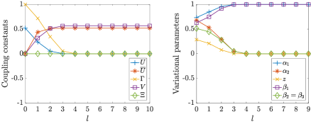
Figure 14: Coupling constants $U(l)$, $\overline{U}(l)$, $\Gamma(l)$, $V(l)$, and $\Xi(l)$ and variational parameters $\alpha_{1}(l)$, $\alpha_{2}(l)$, $z(l)$, $\beta_{1}(l)$, and $\beta_{2}(l)=\beta_{3}(l)$ as functions of $l$ for the bare couplings $U(0)=\overline{U}_{\Gamma(0),\Xi(0)}=0.51773501$, $\Gamma(0)=1$, $V(0)=0$, and $\Xi(0)=0$. The left graph is identical to Fig. 4(b) except that the present figure does not contain $U(l)$ for $U(0)\not=\overline{U}_{\Gamma(0),\Xi(0)}$.

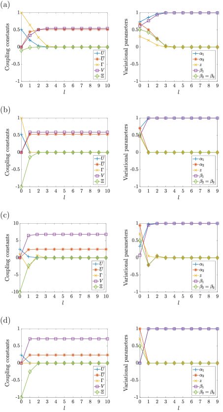
Figure 15: Coupling constants $U(l)$, $\overline{U}(l)$, $\Gamma(l)$, $V(l)$, and $\Xi(l)$ and variational parameters $\alpha_{1}(l)$, $\alpha_{2}(l)$, $z(l)$, $\beta_{1}(l)$, and $\beta_{2}(l)=\beta_{3}(l)$ as functions of $l$ for $\Xi(0)<0$. We set $(U(0),\Gamma(0),V(0),\Xi(0))=(0.51144374,1,0,-0.1)$ in (a), $(0.52956828,1,0,-1)$ in (b), $(2.47583092,1,0,-10)$ in (c), and $(0.23570226,0,0,-1)$ in (d), all of which satisfy $U(0)=\overline{U}_{\Gamma(0),\Xi(0)}$. The left graph of (b) is identical to Fig. 4(a) except that the present figure does not contain $U(l)$ for $U(0)\not=\overline{U}_{\Gamma(0),\Xi(0)}$.

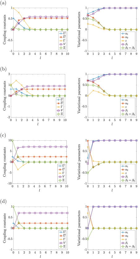
Figure 16: Coupling constants $U(l)$, $\overline{U}(l)$, $\Gamma(l)$, $V(l)$, and $\Xi(l)$ and variational parameters $\alpha_{1}(l)$, $\alpha_{2}(l)$, $z(l)$, $\beta_{1}(l)$, and $\beta_{2}(l)=\beta_{3}(l)$ as functions of $l$ for $\Xi(0)>0$. We set $(U(0),\Gamma(0),V(0),\Xi(0))=(0.52489031,1,0,0.1)$ in (a), $(0.61474501,1,0,1)$ in (b), $(2.46771358,1,0,10)$ in (c), and $(0.23570226,0,0,1)$ in (d), all of which satisfy $U(0)=\overline{U}_{\Gamma(0),\Xi(0)}$. The left graph of (b) is identical to Fig. 4(c) except that the present figure does not contain $U(l)$ for $U(0)\not=\overline{U}_{\Gamma(0),\Xi(0)}$.

Appendix C Derivation of RG equations in the limit of small frustration

We apply the standard real-space RG method Nishimori and Ortiz (2011) to the frustrated Ising ladder (1) in the limit of small frustration, or the limit of a large longitudinal field on the bottom row $U\to\infty$. The model reduces to the ferromagnetic Ising chain with a transverse field and $XX$ interactions (20) after taking the limit $U\to\infty$ and performing the gauge transformation that changes the antiferromagnetic $ZZ$ interactions into ferromagnetic ones.

We partition the chain into $\widetilde{L}=L/2$ blocks and split the Hamiltonian into intrablock and interblock Hamiltonians:

$$\hat{H}=\sum_{I=1}^{\widetilde{L}}(\hat{H}_{I}^{\text{intra}}+\hat{H}_{I,I+1}^{\text{inter}}),$$ (293)

where

$$\hat{H}_{I}^{\text{intra}} =-K\hat{Z}_{2I-1}\hat{Z}_{2I}-\Gamma\hat{X}_{2I-1}-\Xi\hat{X}_{2I-1}\hat{X}_{2I},$$ (294a)

$$\hat{H}_{I,I+1}^{\text{inter}} =-K\hat{Z}_{2I}\hat{Z}_{2I+1}-\Gamma\hat{X}_{2I}-\Xi\hat{X}_{2I}\hat{X}_{2I+1}.$$ (294b)

The intrablock Hamiltonian $\hat{H}_{I}^{\text{intra}}$, which is formed by the ($2I-1$)th and ($2I$)th spins, has the eigenvalues

$$\varepsilon_{s_{1}s_{2}}=-s_{1}\sqrt{K^{2}+\Gamma^{2}}-s_{2}\Xi\quad(s_{1},s_{2}=\pm)$$ (295)

and the corresponding eigenvectors

$$\ket{++} =+c_{+}\ket{\rightarrow\rightarrow}+c_{-}\ket{\leftarrow\leftarrow},$$ (296a)

$$\ket{-+} =-c_{-}\ket{\rightarrow\rightarrow}+c_{+}\ket{\leftarrow\leftarrow},$$ (296b)

$$\ket{+-} =+c_{+}\ket{\rightarrow\leftarrow}+c_{-}\ket{\leftarrow\rightarrow},$$ (296c)

$$\ket{--} =-c_{-}\ket{\rightarrow\leftarrow}+c_{+}\ket{\leftarrow\rightarrow}.$$ (296d)

Here, $\ket{\rightarrow}:=(\ket{\uparrow}+\ket{\downarrow})/\sqrt{2}$ and $\ket{\leftarrow}:=(\ket{\uparrow}-\ket{\downarrow})/\sqrt{2}$ are the eigenvectors of the Pauli operator $\hat{X}$ and

$$c_{\pm}:=\sqrt{\frac{1}{2}\left(1\pm\frac{\Gamma}{\sqrt{K^{2}+\Gamma^{2}}}\right)}.$$ (297)

Now we assume $\lvert\Xi\rvert<\sqrt{K^{2}+\Gamma^{2}}$ and project the Hilbert space onto the two-dimensional low-energy subspace of the intrablock Hamiltonian $\hat{H}_{I}^{\text{intra}}$. Since the two lowest eigenvalues of $\hat{H}_{I}^{\text{intra}}$ are $\varepsilon_{+\pm}$, the projector is given by

$$\hat{Q}=\bigotimes_{I=1}^{\widetilde{L}}\hat{Q}_{I},\quad\hat{Q}_{I}=(\ket{++}\bra{++}+\ket{+-}\bra{+-})_{2I-1,2I}.$$ (298)

Calculating the projections of operators results in

$$\hat{Q}_{I}\hat{H}_{I}^{\text{intra}}\hat{Q}_{I} =\varepsilon_{++}\ket{++}\bra{++}+\varepsilon_{+-}\ket{+-}\bra{+-},$$ (299a)

$$\hat{Q}_{I}\hat{Z}_{2I-1}\hat{Q}_{I} =2c_{+}c_{-}(\ket{+-}\bra{++}+\ket{++}\bra{+-}),$$ (299b)

$$\hat{Q}_{I}\hat{Z}_{2I}\hat{Q}_{I} =\ket{+-}\bra{++}+\ket{++}\bra{+-},$$ (299c)

$$\hat{Q}_{I}\hat{X}_{2I-1}\hat{Q}_{I} =(c_{+}^{2}-c_{-}^{2})(\ket{++}\bra{++}+\ket{+-}\bra{+-}),$$ (299d)

$$\hat{Q}_{I}\hat{X}_{2I}\hat{Q}_{I} =(c_{+}^{2}-c_{-}^{2})(\ket{++}\bra{++}-\ket{+-}\bra{+-}).$$ (299e)

We define $\widetilde{\ket{\uparrow}}:=(\ket{++}+\ket{+-})/\sqrt{2}$ and $\widetilde{\ket{\downarrow}}:=(\ket{++}-\ket{+-})/\sqrt{2}$ and denote the Pauli operators in the basis $\{\,\widetilde{\ket{\sigma}}_{I}\,\}_{\sigma=\uparrow,\downarrow}$ by $\hat{\widetilde{X}}_{I}$, $\hat{\widetilde{Y}}_{I}$, and $\hat{\widetilde{Z}}_{I}$. Then, we obtain the renormalized Hamiltonian $\hat{\widetilde{H}}=\hat{Q}\hat{H}\hat{Q}$ as an operator on the coarse-grained space $\mathop{\mathrm{span}}\{\,\bigotimes_{I=1}^{\widetilde{L}}\widetilde{\ket{\sigma_{I}}}_{I}\,\}_{\sigma_{1},\dots,\sigma_{\widetilde{L}}=\uparrow,\downarrow}$:

$$\hat{\widetilde{H}}=\sum_{I=1}^{\widetilde{L}}(-\widetilde{K}\hat{\widetilde{Z}}_{I}\hat{\widetilde{Z}}_{I+1}-\widetilde{\Gamma}\hat{\widetilde{X}}_{I}-\widetilde{\Xi}\hat{\widetilde{X}}_{I}\hat{\widetilde{X}}_{I+1}),$$ (300)

where we set

$$\widetilde{K} =\frac{K^{2}}{\sqrt{K^{2}+\Gamma^{2}}},$$ (301a)

$$\widetilde{\Gamma} =\frac{\Gamma^{2}}{\sqrt{K^{2}+\Gamma^{2}}}+\Xi\left(1+\frac{\Gamma^{2}}{K^{2}+\Gamma^{2}}\right),$$ (301b)

$$\widetilde{\Xi} =0$$ (301c)

and ignored a constant energy difference. Note that the above choice of the basis $\{\,\widetilde{\ket{\sigma}}_{I}\,\}_{\sigma=\uparrow,\downarrow}$ makes it possible to represent the renormalized Hamiltonian as a summation of the same operators as those in the bare Hamiltonian (20). Finally we derive the RG equations

$$\widetilde{\gamma}=\gamma^{2}+\frac{\xi(1+2\gamma^{2})}{\sqrt{1+\gamma^{2}}},\quad\widetilde{\xi}=0,$$ (302)

where $(\gamma,\xi)=(\Gamma/K,\Xi/K)$ and $(\widetilde{\gamma},\widetilde{\xi})=(\widetilde{\Gamma}/\widetilde{K},\widetilde{\Xi}/\widetilde{K})$.

References

- Kadowaki and Nishimori (1998) T. Kadowaki and H. Nishimori, Quantum annealing in the transverse Ising model, Phys. Rev. E 58, 5355 (1998).
- Brooke et al. (1999) J. Brooke, D. Bitko, T. F., Rosenbaum, and G. Aeppli, Quantum annealing of a disordered magnet, Science 284, 779 (1999).
- Farhi et al. (2001) E. Farhi, J. Goldstone, S. Gutmann, J. Lapan, A. Lundgren, and D. Preda, A quantum adiabatic evolution algorithm applied to random instances of an NP-complete problem, Science 292, 472 (2001).
- Santoro et al. (2002) G. E. Santoro, R. Martoňák, E. Tosatti, and R. Car, Theory of quantum annealing of an Ising spin glass, Science 295, 2427 (2002).
- Santoro and Tosatti (2006) G. E. Santoro and E. Tosatti, Optimization using quantum mechanics: quantum annealing through adiabatic evolution, J. Phys. A 39, R393 (2006).
- Morita and Nishimori (2008) S. Morita and H. Nishimori, Mathematical foundation of quantum annealing, J. Math. Phys. 49, 125210 (2008).
- Albash and Lidar (2018) T. Albash and D. A. Lidar, Adiabatic quantum computation, Rev. Mod. Phys. 90, 015002 (2018).
- Hauke et al. (2020) P. Hauke, H. G. Katzgraber, W. Lechner, H. Nishimori, and W. D. Oliver, Perspectives of quantum annealing: methods and implementations, Rep. Prog. Phys. 83, 054401 (2020).
- Tsuda et al. (2013) J. Tsuda, Y. Yamanaka, and H. Nishimori, Energy gap at first-order quantum phase transitions, J. Phys. Soc. Jpn. 82, 114004 (2013).
- Pfeuty (1970) P. Pfeuty, The one-dimensional Ising model with a transverse field, Ann. Phys. 57, 79 (1970).
- Laumann et al. (2012) C. R. Laumann, R. Moessner, A. Scardicchio, and S. L. Sondhi, Quantum adiabatic algorithm and scaling of gaps at first-order quantum phase transitions, Phys. Rev. Lett. 109, 030502 (2012).
- Jansen et al. (2007) S. Jansen, M.-B. Ruskai, and R. Seiler, Bounds for the adiabatic approximation with applications to quantum computation, J. Math. Phys. 48, 102111 (2007).
- Mozgunov and Lidar (2020) E. Mozgunov and D. A. Lidar, Quantum adiabatic theorem for unbounded Hamiltonians, with applications to superconducting circuits, arXiv:2011.08116 (2020).
- Farhi et al. (2002) E. Farhi, J. Goldstone, and S. Gutmann, Quantum adiabatic evolution algorithms with different paths, arXiv:quant-ph/0208135 (2002).
- Seki and Nishimori (2012) Y. Seki and H. Nishimori, Quantum annealing with antiferromagnetic fluctuations, Phys. Rev. E 85, 051112 (2012).
- Seoane and Nishimori (2012) B. Seoane and H. Nishimori, Many-body transverse interactions in the quantum annealing of the -spin ferromagnet, J. Phys. A 45, 435301 (2012).
- Crosson et al. (2014) E. Crosson, E. Farhi, C. Y.-Y. Lin, H.-h. Lin, and P. Shor, Different strategies for optimization using the quantum adiabatic algorithm, arXiv:1401.7320 (2014).
- Seki and Nishimori (2015) Y. Seki and H. Nishimori, Quantum annealing with antiferromagnetic transverse interactions for the Hopfield model, J. Phys. A 48, 335301 (2015).
- Hormozi et al. (2017) L. Hormozi, E. W. Brown, G. Carleo, and M. Troyer, Nonstoquastic Hamiltonians and quantum annealing of an Ising spin glass, Phys. Rev. B 95, 184416 (2017).
- Nishimori and Takada (2017) H. Nishimori and K. Takada, Exponential enhancement of the efficiency of quantum annealing by non-stoquastic Hamiltonians, Front. ICT 4, 2 (2017).
- Albash (2019) T. Albash, Role of nonstoquastic catalysts in quantum adiabatic optimization, Phys. Rev. A 99, 042334 (2019).
- Takada et al. (2020) K. Takada, Y. Yamashiro, and H. Nishimori, Mean-field solution of the weak-strong cluster problem for quantum annealing with stoquastic and non-stoquastic catalysts, J. Phys. Soc. Jpn. 89, 044001 (2020).
- Matsuura et al. (2021) S. Matsuura, S. Buck, V. Senicourt, and A. Zaribafiyan, Variationally scheduled quantum simulation, Phys. Rev. A 103, 052435 (2021).
- Crosson et al. (2020) E. Crosson, T. Albash, I. Hen, and A. P. Young, De-signing Hamiltonians for quantum adiabatic optimization, Quantum 4, 334 (2020).
- Farhi et al. (2011) E. Farhi, J. Goldstone, D. Gosset, S. Gutmann, H. B. Meyer, and P. Shor, Quantum adiabatic algorithms, small gaps, and different paths, Quantum Inf. Comput. 11, 181 (2011).
- Dickson and Amin (2011) N. G. Dickson and M. H. S. Amin, Does adiabatic quantum optimization fail for NP-complete problems?, Phys. Rev. Lett. 106, 050502 (2011).
- Dickson and Amin (2012) N. G. Dickson and M. H. Amin, Algorithmic approach to adiabatic quantum optimization, Phys. Rev. A 85, 032303 (2012).
- Susa et al. (2018a) Y. Susa, Y. Yamashiro, M. Yamamoto, and H. Nishimori, Exponential speedup of quantum annealing by inhomogeneous driving of the transverse field, J. Phys. Soc. Jpn. 87, 023002 (2018a).
- Mohseni et al. (2018) M. Mohseni, J. Strumpfer, and M. M. Rams, Engineering non-equilibrium quantum phase transitions via causally gapped Hamiltonians, New J. Phys. 20, 105002 (2018).
- Susa et al. (2018b) Y. Susa, Y. Yamashiro, M. Yamamoto, I. Hen, D. A. Lidar, and H. Nishimori, Quantum annealing of the -spin model under inhomogeneous transverse field driving, Phys. Rev. A 98, 042326 (2018b).
- Adame and McMahon (2020) J. I. Adame and P. McMahon, Inhomogeneous driving in quantum annealers can result in orders-of-magnitude improvements in performance, Quantum Sci. Tech. 5, 035011 (2020).
- Perdomo-Ortiz et al. (2010) A. Perdomo-Ortiz, S. E. Venegas-Andraca, and A. Aspuru-Guzik, A study of heuristic guesses for adiabatic quantum computation, Quantum Inf. Proc. 10, 33 (2010).
- Chancellor (2017) N. Chancellor, Modernizing quantum annealing using local searches, New J. Phys. 19, 023024 (2017).
- Ohkuwa et al. (2018) M. Ohkuwa, H. Nishimori, and D. A. Lidar, Reverse annealing for the fully connected -spin model, Phys. Rev. A 98, 022314 (2018).
- Yamashiro et al. (2019) Y. Yamashiro, M. Ohkuwa, H. Nishimori, and D. A. Lidar, Dynamics of reverse annealing for the fully-connected -spin model, Phys. Rev. A 100, 052321 (2019).
- King et al. (2018) A. D. King, J. Carrasquilla, J. Raymond, I. Ozfidan, E. Andriyash, A. Berkley, M. Reis, T. Lanting, R. Harris, F. Altomare, K. Boothby, P. I. Bunyk, C. Enderud, A. Fréchette, E. Hoskinson, N. Ladizinsky, T. Oh, G. Poulin-Lamarre, C. Rich, Y. Sato, A. Y. Smirnov, L. J. Swenson, M. H. Volkmann, J. Whittaker, J. Yao, E. Ladizinsky, M. W. Johnson, J. Hilton, and M. H. Amin, Observation of topological phenomena in a programmable lattice of 1,800 qubits, Nature 560, 456 (2018).
- Ottaviani and Amendola (2018) D. Ottaviani and A. Amendola, Low rank non-negative matrix factorization with D-Wave 2000Q, arXiv:1808.08721 (2018).
- Marshall et al. (2019) J. Marshall, D. Venturelli, I. Hen, and E. G. Rieffel, Power of pausing: Advancing understanding of thermalization in experimental quantum annealers, Phys. Rev. Appl. 11, 044083 (2019).
- Venturelli and Kondratyev (2019) D. Venturelli and A. Kondratyev, Reverse quantum annealing approach to portfolio optimization problems, Quantum Mach. Intell. 1, 17 (2019).
- Ikeda et al. (2019) K. Ikeda, Y. Nakamura, and T. S. Humble, Application of quantum annealing to nurse scheduling problem, Sci. Rep. 9, 12837 (2019).
- Rocutto et al. (2021) L. Rocutto, C. Destri, and E. Prati, Quantum semantic learning by reverse annealing of an adiabatic quantum computer, Adv. Quantum Technol. 4, 2000133 (2021).
- Passarelli et al. (2020) G. Passarelli, K.-W. Yip, D. A. Lidar, H. Nishimori, and P. Lucignano, Reverse quantum annealing of the -spin model with relaxation, Phys. Rev. A 101, 022331 (2020).
- Arai et al. (2021) S. Arai, M. Ohzeki, and K. Tanaka, Mean field analysis of reverse annealing for code-division multiple-access multiuser detection, Phys. Rev. Res. 3, 033006 (2021).
- Passarelli et al. (2019) G. Passarelli, V. Cataudella, and P. Lucignano, Improving quantum annealing of the ferromagnetic -spin model through pausing, Phys. Rev. B 100, 024302 (2019).
- Kadowaki and Ohzeki (2019) T. Kadowaki and M. Ohzeki, Experimental and theoretical study of thermodynamic effects in a quantum annealer, J. Phys. Soc. Jpn. 88, 061008 (2019).
- Chen and Lidar (2020) H. Chen and D. A. Lidar, Why and when pausing is beneficial in quantum annealing, Phys. Rev. Appl. 14, 014100 (2020).
- Crosson and Lidar (2021) E. J. Crosson and D. A. Lidar, Prospects for quantum enhancement with diabatic quantum annealing, Nature Rev. Phys. 3, 466 (2021).
- Bravyi et al. (2008) S. Bravyi, D. P. DiVincenzo, R. Oliveira, and B. M. Terhal, The complexity of stoquastic local Hamiltonian problems, Quantum Inf. Comput. 8, 361 (2008).
- Loh et al. (1990) E. Y. Loh, J. E. Gubernatis, R. T. Scalettar, S. R. White, D. J. Scalapino, and R. L. Sugar, Sign problem in the numerical simulation of many-electron systems, Phys. Rev. B 41, 9301 (1990).
- Gupta and Hen (2019) L. Gupta and I. Hen, Elucidating the interplay between non-stoquasticity and the sign problem, arXiv:1910.13867 (2019).
- Marvian et al. (2019) M. Marvian, D. A. Lidar, and I. Hen, On the computational complexity of curing non-stoquastic Hamiltonians, Nat. Commun. 10, 1571 (2019).
- Klassen et al. (2020) J. Klassen, M. Marvian, S. Piddock, M. Ioannou, I. Hen, and B. M. Terhal, Hardness and ease of curing the sign problem for two-local qubit Hamiltonians, SIAM J. Comput. 49, 1332 (2020).
- Halverson et al. (2020) T. Halverson, L. Gupta, M. Goldstein, and I. Hen, Efficient simulation of so-called non-stoquastic superconducting flux circuits, arXiv:2011.03831 (2020).
- Suzuki (1976) M. Suzuki, Relationship between -dimensional quantal spin systems and ()-dimensional Ising systems, Prog. Theor. Phys. 56, 1454 (1976).
- Aharonov et al. (2007) D. Aharonov, W. van Dam, J. Kempe, Z. Landau, S. Lloyd, and O. Regev, Adiabatic quantum computation is equivalent to standard quantum computation, SIAM J. Comput. 37, 166 (2007).
- Mizel et al. (2007) A. Mizel, D. A. Lidar, and M. Mitchell, Simple proof of equivalence between adiabatic quantum computation and the circuit model, Phys. Rev. Lett. 99, 070502 (2007).
- Gosset et al. (2015) D. Gosset, B. M. Terhal, and A. Vershynina, Universal adiabatic quantum computation via the space-time circuit-to-Hamiltonian construction, Phys. Rev. Lett. 114, 140501 (2015).
- Jordan et al. (2010) S. P. Jordan, D. Gosset, and P. J. Love, Quantum-Merlin-Arthur–complete problems for stoquastic Hamiltonians and Markov matrices, Phys. Rev. A 81, 032331 (2010).
- Bravyi et al. (2006) S. Bravyi, A. J. Bessen, and B. M. Terhal, Merlin-Arthur games and stoquastic complexity, arXiv:quant-ph/0611021 (2006).
- Hastings (2020) M. B. Hastings, The power of adiabatic quantum computation with no sign problem, arXiv:2005.03791 (2020).
- Gilyén et al. (2021) A. Gilyén, M. B. Hastings, and U. Vazirani, (Sub)exponential advantage of adiabatic quantum computation with no sign problem, in Proceedings of the 53rd Annual ACM SIGACT Symposium on Theory of Computing (STOC) (2021) pp. 1357–1369.
- Jonathan and Plenio (1999) D. Jonathan and M. B. Plenio, Entanglement-assisted local manipulation of pure quantum states, Phys. Rev. Lett. 83, 3566 (1999).
- Biamonte and Love (2008) J. D. Biamonte and P. J. Love, Realizable Hamiltonians for universal adiabatic quantum computers, Phys. Rev. A 78, 012352 (2008).
- (64) K. Takada and D. A. Lidar, unpublished .
- Nishimori and Ortiz (2011) H. Nishimori and G. Ortiz, Elements of Phase Transitions and Critical Phenomena (Oxford University Press, Oxford, United Kingdom, 2011).
- Sachdev (2011) S. Sachdev, Quantum Phase Transitions, 2nd ed. (Cambridge University Press, Cambridge, United Kingdom, 2011).
- Langari (1998) A. Langari, Phase diagram of the antiferromagnetic XXZ model in the presence of an external magnetic field, Phys. Rev. B 58, 14467 (1998).
- Langari (2004) A. Langari, Quantum renormalization group of model in a transverse magnetic field, Phys. Rev. B 69, 100402(R) (2004).
- White (1992) S. R. White, Density matrix formulation for quantum renormalization groups, Phys. Rev. Lett. 69, 2863 (1992).
- White (1993) S. R. White, Density-matrix algorithms for quantum renormalization groups, Phys. Rev. B 48, 10345 (1993).
- Schollwöck (2005) U. Schollwöck, The density-matrix renormalization group, Rev. Mod. Phys. 77, 259 (2005).
- Hallberg (2006) K. A. Hallberg, New trends in density matrix renormalization, Adv. Phys. 55, 477 (2006).
- Feynman (1939) R. P. Feynman, Forces in molecules, Phys. Rev. 56, 340 (1939).