Layer pseudospin dynamics and genuine non-Abelian Berry phase in inhomogeneously strained moiré pattern

Abstract

Periodicity of long wavelength moiré patterns is very often destroyed by the inhomogeneous strain introduced in fabrications of van der Waals layered structures. We present a framework to describe massive Dirac fermions in such distorted moiré pattern of transition metal dichalcogenides homobilayers, accounting for the dynamics of layer pseudospin. In decoupled bilayers, we show two causes of in-plane layer pseudospin precession: By the coupling of layer antisymmetric strain to valley magnetic moment; and by the Aharonov-Bohm effect in the SU(2) gauge potential for the case of R-type bilayer under antisymmetric strain and H-type under symmetric strain. With interlayer coupling in the moiré, its interplay with strain manifests as a non-Abelian gauge field. We show a genuine non-Abelian Aharonov-Bohm effect in such field, where the evolution operators for different loops are non-commutative. This provides an exciting platform to explore non-Abelian gauge field effects on electron, with remarkable tunability of the field by strain and interlayer bias.

Long-wavelength moiré patterns by van der Waals stacking of graphene and transition metal dichalcogenides (TMDs) have led to the observation of a plethora of novel electron correlation phenomena Cao et al. (2018a, b); Sharpe et al. (2019); Yankowitz et al. (2019); Serlin et al. (2020); Lu et al. (2019); Tang et al. (2020); Regan et al. (2020); Shimazaki et al. (2020), as well as moiré excitons as highly tunable quantum emitters Yu et al. (2017); Seyler et al. (2019); Tran et al. (2019); Jin et al. (2019); Alexeev et al. (2019); Jauregui et al. (2019). In these findings, the moiré pattern is exploited as a superlattice energy landscape to trap electrons and excitons, arising from the spatially modulated interlayer coupling Zhang et al. (2017). Theoretical studies revealed that interlayer coupling in the moiré manifests as a location dependent Zeeman field on the layer pseudospin (e.g. Fig. 1), which exhibits a skyrmion texture in real space Wu et al. (2019); Yu et al. (2020); Zhai and Yao (2020). For holes, Berry curvature from the adiabatic motion in such moiré field is an Abelian gauge field that realizes fluxed superlattices Yu et al. (2020); Zhai and Yao (2020), underlying the quantum spin Hall effect discovered in low energy mini-bands Wu et al. (2019); Bi et al. (2019). Link between moiré induced gauge field on massless Dirac fermions and flattening of mini-bands in twisted bilayer graphene have also been explored Wolf et al. (2019); Liu et al. (2019); San-Jose et al. (2012). For electrons in homobilayer TMDs, the moiré field has similar spatial texture but is much weaker at certain spots in the supercell [Figs. 1(b–c)] Wang et al. (2017), where non-adiabatic pseudospin dynamics need to be accounted. This points to the relevance of intriguing SU(2) Berry phases on massive particles in the moiré. In particular, genuine non-Abelian gauge field– origin of the noncommutativity of successive loop operations– in real space is of great interest Goldman et al. (2014), but has only been realized recently in synthetic optical systems Yang et al. (2019).

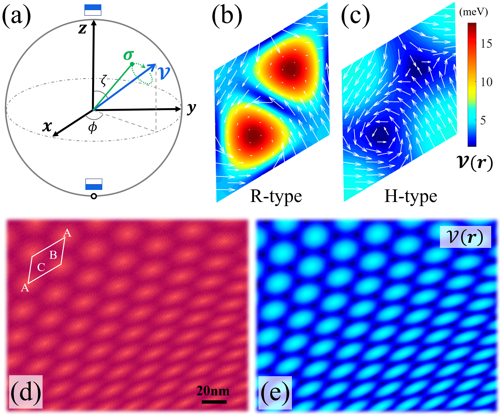
Figure 1: Effective moiré field and strained moiré pattern. (a) Schematics of layer pseudospin $\boldsymbol{\sigma}$ (green line) precessing around the moiré field $\boldsymbol{\mathcal{V}}$ (blue arrow). (b) Color map plots $\mathcal{V}$ in a rigid moiré unit cell, for valley electrons in R-type twisted bilayer MoSe₂. Arrows denote the in-plane components of $\hat{\boldsymbol{\mathcal{V}}}$. (c) Same plot for H-type MoS₂. (d) An example of strained moiré pattern (adapted from Ref. Bai et al. (2020)). The parallelogram denotes a distorted moiré cell. (e) The moiré field of (c) mapped onto such distorted moiré pattern.

In experimental reality, inhomogeneous strain is often unintentionally introduced van der Zande et al. (2014); Bai et al. (2020). In monolayers, strain can be described by a pseudo-vector potential with valley contrasted signs, which is associated with an effective magnetic field when strain is inhomogeneous Amorim et al. (2016). In the moiré, dramatic distortion of the periodic landscape occurs in the presence of layer dependent heterostrain Tong et al. (2017). Fig. 1(d) is an example of a $0.86^{\circ}$ twisted moiré subject to inhomogeneous heterostrain of peak magnitude $\sim 0.5\%$, where the moiré wavelength varies appreciably over a few periods. For carrier dynamics in such moiré, the momentum space description in terms of mini-bands is not validated with the broken periodicity.

Here we present a framework to describe massive Dirac fermions with the non-adiabatic layer pseudospin dynamics in inhomogeneously distorted TMD homobilayer moiré. We first outline several Abelian SU(2) Berry phase effects purely from the layer symmetric and antisymmetric components of strain under R-type (parallel) and H-type (antiparallel) stacking. Coupling of the electron’s valley magnetic moment to the strain induced magnetic field causes in-plane precession of the pseudospin in layer antisymmetric strain. Moreover, R-type (H-type) bilayer under antisymmetric (symmetric) strain features a SU(2) gauge potential in which the Aharonov-Bohm (AB) interference also manifests as in-plane pseudospin precession. When interlayer coupling is considered, its interplay with the strain can be formulated in terms of a non-Abelian gauge field, whose matrix forms at different locations are noncommutative. Evolution in this field has the genuine non-Abelian AB effect where the evolution operators for different loops are noncommutative Goldman et al. (2014).

In a long wavelength moiré subject to a general strain pattern, the low energy carriers are described by the continuum Hamiltonian Bi et al. (2019); Zhai and Yao (2020); Koshino and Nam (2020)

$$\mathcal{H}=\begin{pmatrix}v\boldsymbol{\pi}_{t}\cdot\boldsymbol{\sigma}^{\prime}_{\tau^{t}}+\frac{E_{g}}{2}\sigma^{\prime}_{z}+V^{t}&U\\ U^{\dagger}&v\boldsymbol{\pi}_{b}\cdot\boldsymbol{\sigma}^{\prime}_{\tau^{b}}+\frac{E_{g}}{2}\sigma^{\prime}_{z}+V^{b}\end{pmatrix}$$ (1)

with $\boldsymbol{\pi}_{l}=\mathbf{p}+\tau^{l}\mathbf{A}^{l}_{\epsilon}$, $l=t,b$ the layer index, and $\tau^{l}=\pm$ the valley index in layer $l$. The effect of strain (tensor $\epsilon_{ij}$) is accounted by the vector potential $\mathbf{A}^{l}_{\epsilon}=\frac{\sqrt{3}\hbar\beta}{2a}(\epsilon^{l}_{xx}-\epsilon^{l}_{yy},\,-2\epsilon^{l}_{xy})$ Sup , where $a$ is the lattice constant, and $\beta\approx 2-3$ Fang et al. (2018). $\boldsymbol{\sigma}^{\prime}_{\tau^{l}}=(\tau^{l}\sigma^{\prime}_{x},\,\sigma^{\prime}_{y})$ and $\sigma^{\prime}_{z}$ are Pauli matrices spanned by the metal d orbitals at the conduction ($c$) and valence ($v$) band edges Xiao et al. (2012). $V^{l}=\text{diag}(\tilde{V}^{l}_{c},\,\tilde{V}^{l}_{v})$ and $U=\begin{pmatrix}\tilde{U}_{cc}&\tilde{U}_{cv}\\ \tilde{U}_{vc}&\tilde{U}_{vv}\end{pmatrix}$ accounts for the interlayer coupling, which are functions of interlayer registry with location dependence Yu et al. (2020); Zhai and Yao (2020); Wu et al. (2019); Wang et al. (2017). Because $U$ couples only states of the same spin [Fig. 2(a)], we consider one spin species per valley at a time.

The large band gap $E_{g}$ allows one to perturbatively eliminate the valence bands Wu et al. (2019); Yu et al. (2020); Zhai and Yao (2020), to reach a reduced Hamiltonian on the electron

$$H=\frac{1}{2m}\left(\mathbf{p}+\boldsymbol{\mathcal{A}}_{\epsilon}\right)^{2}+\mathcal{U}+\mathcal{Z}_{\epsilon}.$$ (2)

It has a $2\times 2$ matrix form, spanned by the layer pseudospin $\boldsymbol{\sigma}$. $\boldsymbol{\mathcal{A}}_{\epsilon}=\text{diag}(\tau^{t}\mathbf{A}^{t}_{\epsilon},\,\tau^{b}\mathbf{A}^{b}_{\epsilon})$ is the matrix of strain induced vector potential. Hereafter, we focus on the $\tau^{t}=+$ valley of the top layer, which is coupled with the $\tau^{b}=+$ ($-$) valley of the lower layer in the parallel (antiparallel) stacking [Fig. 2(a)]. Results for the other valley can be obtained by time-reversal symmetry.

The term $\mathcal{U}=\begin{pmatrix}\tilde{V}^{t}_{c}&\tilde{U}_{cc}\\ \tilde{U}^{*}_{cc}&\tilde{V}^{b}_{c}\end{pmatrix}$ is responsible for the moiré potential and layer hybridization of the carriers Wu et al. (2019); Yu et al. (2020); Zhai and Yao (2020); Sup . We can write $\mathcal{U}=\mathcal{V}_{0}\sigma_{0}+\boldsymbol{\sigma}\cdot\boldsymbol{\mathcal{V}}$, where $\sigma_{0}$ is the identity matrix. $\boldsymbol{\mathcal{V}}$ is an effective field that causes the layer pseudospin precession [Fig. 1(a)]. Figs. 1(b–c) plot its magnitude and in-plane texture in a moiré unit cell showing the strong location dependence, in R- and H-type TMD bilayer examples, respectively.

$\mathcal{Z}_{\epsilon}$ is the Zeeman energy of the valley magnetic moment in the strain induced pseudomagnetic field $\boldsymbol{\mathcal{B}}_{\epsilon}=\frac{1}{e}\nabla\times\boldsymbol{\mathcal{A}}_{\epsilon}$. In monolayers, Dirac electron of effective mass $m$ carries an intrinsic magnetic moment $\tau\mu_{B}^{*}=\tau\frac{e\hbar}{2m}$ in out-of-plane direction Xiao et al. (2007). Interestingly, out of the three contributions to the magnetic moment in TMDs Aivazian et al. (2015), the pseudomagnetic field couples only to this lattice contribution associated with the Berry phase, but not those from spin and atomic orbitals. We can write $\mathcal{Z}_{\epsilon}=\boldsymbol{\mu}\cdot\boldsymbol{\mathcal{B}}_{\epsilon}$, where valley magnetic moment $\boldsymbol{\mu}$ is listed in Table 1.

Table 1: R-type vs H-type bilayer TMDs with inhomogeneous strain. $B^{\alpha}_{\epsilon}\hat{\bf z}=\frac{1}{e}\nabla\times\mathbf{A}^{\alpha}_{\epsilon}$, $Z^{\alpha}_{\epsilon}=\mu_{B}^{*}B^{\alpha}_{\epsilon}$, $\alpha=a,s$.

	$\boldsymbol{\mu}$	$\boldsymbol{\mathcal{A}}_{\epsilon}^{s}$	$\boldsymbol{\mathcal{A}}_{\epsilon}^{a}$	$\boldsymbol{\mathcal{B}}_{\epsilon}^{s}$	$\boldsymbol{\mathcal{B}}_{\epsilon}^{a}$	$\mathcal{Z}_{\epsilon}^{s}$	$\mathcal{Z}_{\epsilon}^{a}$
R-type	$\mu_{B}^{*}\hat{\bf z}\sigma_{0}$	$\mathbf{A}^{s}_{\epsilon}\sigma_{0}$	$\mathbf{A}^{a}_{\epsilon}\sigma_{z}$	$B^{s}_{\epsilon}\hat{\bf z}\sigma_{0}$	$B^{a}_{\epsilon}\hat{\bf z}\sigma_{z}$	$Z^{s}_{\epsilon}\sigma_{0}$	$Z^{a}_{\epsilon}\sigma_{z}$
H-type	$\mu_{B}^{*}\hat{\bf z}\sigma_{z}$	$\mathbf{A}^{s}_{\epsilon}\sigma_{z}$	$\mathbf{A}^{a}_{\epsilon}\sigma_{0}$	$B^{s}_{\epsilon}\hat{\bf z}\sigma_{z}$	$B^{a}_{\epsilon}\hat{\bf z}\sigma_{0}$	$Z^{s}_{\epsilon}\sigma_{0}$	$Z^{a}_{\epsilon}\sigma_{z}$

Using $\mathbf{A}^{s}_{\epsilon}\equiv(\mathbf{A}^{t}_{\epsilon}+\mathbf{A}^{b}_{\epsilon})/2$ and $\mathbf{A}^{a}_{\epsilon}\equiv(\mathbf{A}^{t}_{\epsilon}-\mathbf{A}^{b}_{\epsilon})/2$ to quantify the layer symmetric (s) and antisymmetric (a) parts of a general strain in bilayer, one decomposes $\boldsymbol{\mathcal{A}}_{\epsilon}=\boldsymbol{\mathcal{A}}_{\epsilon}^{s}+\boldsymbol{\mathcal{A}}_{\epsilon}^{a}$, as well as $\boldsymbol{\mathcal{B}}_{\epsilon}$. The Hamiltonian then reads $H=\frac{1}{2m}\left(\mathbf{p}+\boldsymbol{\mathcal{A}}_{\epsilon}^{s}+\boldsymbol{\mathcal{A}}_{\epsilon}^{a}\right)^{2}+\mathcal{U}+\mathcal{Z}_{\epsilon}^{s}+\mathcal{Z}_{\epsilon}^{a}$. Table 1 summarizes the pseudospin dependence of these physical quantities. $\sigma_{0}$ vs $\sigma_{z}$ reflect the parallel vs antiparallel stacking in R-type and H-type bilayers. $\sigma_{z}$ marks the layer contrasted sign of the quantities, which will affect pseudospin dynamics as discussed next.

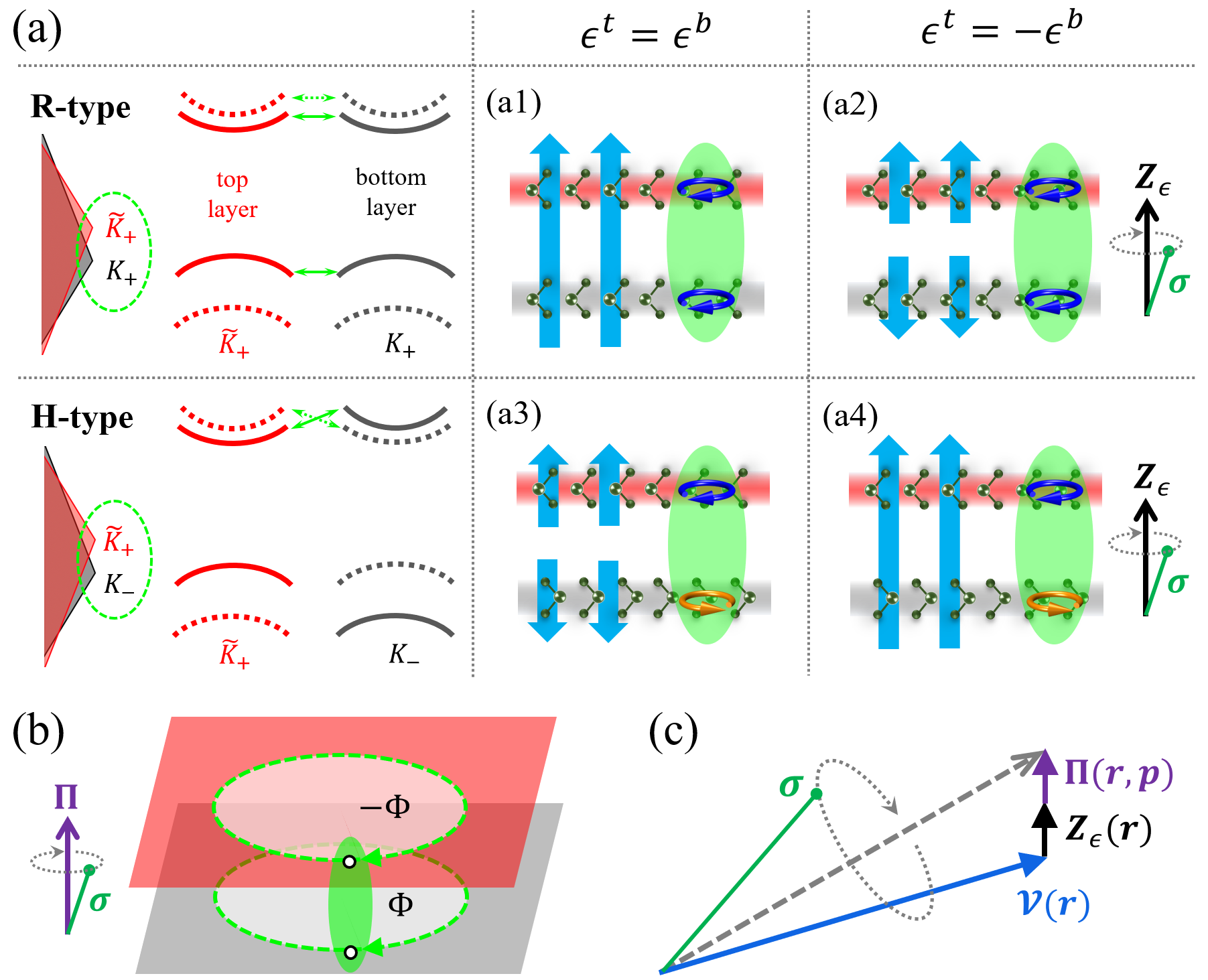
Figure 2: Comparison of twisted homobilayer TMD (e.g. MoX₂) with different stacking and strain configurations. (a) First column: Monolayer Brillouin corners for R-type (upper) and H-type (lower) twisted bilayer. The dashed circles highlight the two coupled Dirac cones. Solid and dotted curves represent spin-split Dirac cones. Double-head arrows denote interlayer coupling. (a1) & (a3): Strain induced pseudomagnetic field (wide blue arrows) and valley magnetic moment (curly arrows) for layer symmetric strain ($\epsilon^{t}=\epsilon^{b}$) in R-type (upper) and H-type (lower) bilayer, respectively. (a2) & (a4): Same as before but with layer antisymmetric strain ($\epsilon^{t}=-\epsilon^{b}$). Green stick and black arrow illustrate layer pseudospin precession around the strain Zeeman field $\mathbf{Z}_{\epsilon}$. (b) Pseudospin precession around $\boldsymbol{\Pi}$ in the presence of layer contrasted pseudomagnetic field. The AB phases gained in the two layers are opposite ($\pm\Phi$) when a particle evolves in a loop. (c) Schematics showing the pseudospin precessing around the net effective Zeeman field (gray dashed arrow) in the presence of both strain and moiré coupling.

Remarkably, the two strain components, combined with the strain dependent valley magnetic moment $\boldsymbol{\mu}$, lead to four distinct scenarios of the pseudospin dynamics. First, in the Zeeman term, it is the antisymmetric strain that leads to the splitting of the layer pseudospin in either bilayer stacking [Table 1 last column, and Figs. 2(a2) & (a4)]. Moreover, the geometric phase in the centre-of-mass (COM) motion due to layer contrasted pseudomagnetic field [wide blue arrows pointing oppositely in Figs. 2(a2) & (a3), i.e. R-type (H-type) bilayer under antisymmetric (symmetric) strain] is another cause of pseudospin precession. Upon closing a loop in such fields, electron picks up opposite geometric phases $e^{\mp ie\Phi/\hbar}$ in its two layer components, resulting in an in-plane rotation of pseudospin [Fig. 2(b)], which is the AB effect in a SU(2) gauge field first discussed by Wu and Yang Wu and Yang (1975).

The above effects on pseudospin can be explicitly seen from its Heisenberg equation of motion,

$$\dot{\boldsymbol{\sigma}}=-\frac{i}{\hbar}[H,\boldsymbol{\sigma}]=\frac{2}{\hbar}\left(\boldsymbol{\Pi}_{\epsilon}+\boldsymbol{\mathcal{K}}_{\epsilon}+\mathbf{Z}^{a}_{\epsilon}+\boldsymbol{\mathcal{V}}\right)\times\boldsymbol{\sigma}.$$ (3)

$\boldsymbol{\Pi}_{\epsilon}=\frac{1}{2m}(\mathbf{p}\cdot\mathbf{A}^{\alpha}_{\epsilon}+\mathbf{A}^{\alpha}_{\epsilon}\cdot\mathbf{p})\hat{\bf z}$, $\alpha=a/s$ for R-/H-type, reflects a pseudospin precession accompanying the COM motion. The aforementioned AB effect [Fig. 2(b)] is a manifestation of this term. $\mathbf{Z}^{a}_{\epsilon}=Z^{a}_{\epsilon}\hat{\bf z}$ is from the Zeeman splitting in the antisymmetric strain (last column of Table 1). $\boldsymbol{\mathcal{K}}_{\epsilon}=\frac{1}{m}\mathbf{A}^{s}_{\epsilon}\cdot\mathbf{A}^{a}_{\epsilon}\hat{\bf z}$ is a cross term between symmetric and antisymmetric strain components, which is negligible under modest strain. $\mathbf{Z}^{a}_{\epsilon}$ is function of location, while $\boldsymbol{\Pi}_{\epsilon}$ also depends on momentum, both pointing out-of-plane. In a strain of $\epsilon\sim 1\%$ and at Fermi wavelength $\lambda_{f}\sim 2$ nm (corresponding to Fermi energy of $\sim 20$ meV in TMDs), $\Pi_{\epsilon}\sim\frac{\hbar^{2}}{2ma}\frac{\epsilon}{\lambda_{F}}\sim 1$ meV. And for strain variation $\Delta\epsilon\sim 1\%$ over a length $l\sim 10$ nm, $Z^{a}_{\epsilon}\sim\frac{\hbar^{2}}{2ma}\frac{\Delta\epsilon}{l}\sim 0.2$ meV.

In comparison, $\boldsymbol{\mathcal{V}}$ from the interlayer coupling has its orientation vary spatially [Figs. 1(b–c)], determined by the local atomic registry in the moiré Zhai and Yao (2020); Yu et al. (2020); Wu et al. (2019). Its magnitude $\mathcal{V}\sim$ O(1) meV at certain spots, and reaches O(10) meV over the rest area in the moiré, well exceeding that of $\boldsymbol{\Pi}_{\epsilon}$ and $\mathbf{Z}_{\epsilon}^{a}$. Fig. 2(c) illustrates the collective effect of these non-collinear pseudo-fields from both interlayer coupling and strain. As we show below, their interplay leads to genuine non-Abelian Berry phase effects that are absent with either moiré coupling or strain alone.

Non-Abelian Berry curvature - As the pseudospin dynamics is dominated by the interlayer coupling, it is natural to switch to the basis of its local eigenstates, satisfying $\boldsymbol{\sigma}\cdot\boldsymbol{\mathcal{V}}\ket{\chi_{\pm}(\bf{r})}=\pm\mathcal{V}\ket{\chi_{\pm}(\bf{r})}$. The Hamiltonian in this basis reads

$$\tilde{H}=Q^{\dagger}HQ=\frac{1}{2m}\left(\mathbf{p}+\boldsymbol{\mathcal{A}}\right)^{2}+E_{c}+\mathcal{\tilde{Z}}_{\epsilon},$$ (4)

where $Q=\left(|\chi_{+}\rangle,\,|\chi_{-}\rangle\right)$. The interlayer coupling is diagonalised, i.e. $E_{c}=\text{diag}(\mathcal{V}_{0}+\mathcal{V},\,\mathcal{V}_{0}-\mathcal{V})$, which characterises the scalar moiré potential experienced by the two pseudospin branches Yu et al. (2020). The gauge potential is now a composite one $\boldsymbol{\mathcal{A}}=\boldsymbol{\mathcal{A}}_{\nabla}+\boldsymbol{\mathcal{\tilde{A}}}_{\epsilon}$. The first part is due to the transformation in the non-Abelian group Xiao et al. (2010), $\boldsymbol{\mathcal{A}}_{\nabla}=-i\hbar Q^{\dagger}\nabla Q=-\frac{\hbar}{2}\left(\nabla\phi\right)\tilde{\sigma}_{z}+\frac{\hbar}{2}\left(\nabla\zeta\right)\sigma_{y}$, where $\zeta(\bf{r})$ and $\phi(\bf{r})$ are the polar and azimuthal angles of the local $\boldsymbol{\mathcal{V}}$ respectively [Fig. 1(a)], and $\tilde{\sigma}_{z}\equiv Q^{\dagger}\sigma_{z}Q=\sigma_{z}\cos\zeta+\sigma_{x}\sin\zeta$. Its explicit form is gauge dependent and we adapt the one in Ref. Zhai and Yao (2020). The second part is from the strain, $\boldsymbol{\mathcal{\tilde{A}}}_{\epsilon}=Q^{\dagger}\boldsymbol{\mathcal{A}}_{\epsilon}Q=\mathbf{A}^{\alpha_{1}}_{\epsilon}\sigma_{0}+\mathbf{A}^{\alpha_{2}}_{\epsilon}\tilde{\sigma}_{z}$, where $\alpha_{1}=s$ ($a$) and $\alpha_{2}=a$ ($s$) for R-type (H-type) bilayers (see Table 1). The associated gauge field reads Goldman et al. (2014); Xiao et al. (2010)

$$\boldsymbol{\mathcal{B}}=\frac{1}{e}\nabla\times\boldsymbol{\mathcal{A}}+\frac{i}{e\hbar}[\mathcal{A}_{x},\mathcal{A}_{y}]\hat{\bf z}=(B^{\alpha_{1}}_{\epsilon}\sigma_{0}+B^{\alpha_{2}}_{\epsilon}\tilde{\sigma}_{z})\hat{\bf z}.$$ (5)

It corresponds to a transformation of the strain induced pseudomagnetic field $\boldsymbol{\mathcal{B}}=Q^{\dagger}\boldsymbol{\mathcal{B}}_{\epsilon}Q$ (Table 1). The Zeeman coupling of the valley magnetic moment to $\boldsymbol{\mathcal{B}}$ appears as the last term in Eq. (4), $\mathcal{\tilde{Z}}_{\epsilon}=Z^{s}_{\epsilon}\sigma_{0}+Z^{a}_{\epsilon}\tilde{\sigma}_{z}$.

The non-Abelian nature of the gauge field is evidenced from its noncommutativity at different locations: $\left[\boldsymbol{\mathcal{B}}(\mathbf{r}),\boldsymbol{\mathcal{B}}(\mathbf{r}^{\prime})\right]=2i\sigma_{y}\text{B}^{\alpha_{2}}_{\epsilon}(\mathbf{r})\text{B}^{\alpha_{2}}_{\epsilon}(\mathbf{r}^{\prime})\sin\left(\zeta(\mathbf{r}^{\prime})-\zeta(\mathbf{r})\right)$. This is endowed by the fact that the interlayer hopping $\mathcal{V}_{x}\sigma_{x}+\mathcal{V}_{y}\sigma_{y}$ varies spatially in the moiré, and does not commute with the strain induced $\boldsymbol{\mathcal{A}}_{\epsilon}$ with a $\sigma_{z}$ part. We can compare with situations where only either of the above causes is present. In the limit $\epsilon=0$, the gauge potential $\boldsymbol{\mathcal{A}}=\boldsymbol{\mathcal{A}}_{\nabla}$ is non-Abelian, but the gauge field simply vanishes Zhai and Yao (2020). In the limit of decoupled layers, $\zeta(\mathbf{r})=0$, the gauge field reduces to $\boldsymbol{\mathcal{B}}_{\epsilon}(\mathbf{r})$ whose forms at different locations always commute. In aligned bilayers, the ratio of interlayer hopping to the band offset ($\mathcal{V}_{z}$) is spatially uniform rendering $\zeta(\mathbf{r})$ constant, which also ensures that $\boldsymbol{\mathcal{B}}$ at different locations commute. Indeed, the moiré pattern combined with the inhomogeneous strain creates a unique scenario for the genuine non-Abelian gauge field to emerge.

A force operator can also be defined to illustrate the effects of the non-Abelian Berry phase effect on the COM motion: $\boldsymbol{\mathcal{F}}=m\dot{\mathbf{v}}=-\frac{i}{\hbar}[m\mathbf{v},\tilde{H}]=-\frac{e}{2}\left(\mathbf{v}\times\boldsymbol{\mathcal{B}}-\boldsymbol{\mathcal{B}}\times\mathbf{v}\right)-\nabla\left(E_{c}+\mathcal{\tilde{Z}}_{\epsilon}\right)-\frac{i}{\hbar}[\boldsymbol{\mathcal{A}},E_{c}+\mathcal{\tilde{Z}}_{\epsilon}]$, where $\mathbf{v}=-\frac{i}{\hbar}[\mathbf{r},\tilde{H}]=\frac{1}{m}\left(\mathbf{p}+\boldsymbol{\mathcal{A}}\right)$ is the velocity operator. The first term is the magnetic force by the non-Abelian gauge field, while the rest two terms are reminiscent of electric force Goldman et al. (2014). For comparison, in an unstrained moiré superlattice, the force reads $\boldsymbol{\mathcal{F}}_{\epsilon=0}=-\nabla E_{c}-\frac{i}{\hbar}[\boldsymbol{\mathcal{A}}_{\nabla},E_{c}]$ without the magnetic part.

Fig. 3 gives an example of the non-Abelian gauge field for H-type bilayer MoS₂ featuring the moiré pattern shown in Fig. 1(c). The non-periodic moiré is produced by a $0.86^{\circ}$ twisting and a modest layer antisymmetric strain with peak magnitude $\epsilon^{a}\sim 0.5\%$ Sup . Oftentimes, inhomogeneous heterostrain of this magnitude is unintentionally introduced in the fabrication of moiré lattices Bai et al. (2020). Interestingly, such system naturally provides a platform for studying noncommutative phenomena.

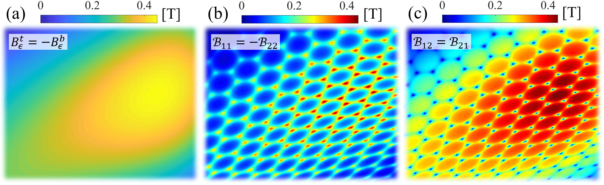
Figure 3: Strain pseudomagnetic field and non-Abelian gauge field in strained H-type $0.86^{\circ}$ twisted bilayer MoS₂. (a) $B^{t}_{\epsilon}=-B^{b}_{\epsilon}$. (b) $\mathcal{B}_{11}=-\mathcal{B}_{22}$. (c) $\mathcal{B}_{12}=\mathcal{B}_{21}$.

The moiré lattice and strain can also be independently controlled to engineer the non-Abelian gauge field. Stress of various forms can be applied first on the bottom layer using movable substrates Mikael et al. (2017), before the top layer is deposited with the control of twisting angle. Strain can also be introduced by depositing 2D materials on pre-engineered substrates with tailorable shapes and sizes Nigge et al. (2019); Jiang et al. (2017). Fig. 4 illustrates an example of R-type bilayer MoSe₂, whose bottom layer is triaxially strained over a circular area Sup . Fig. 4(b) plots the interlayer coupling $\boldsymbol{\mathcal{V}}(\bf{r})$ in the strain distorted moiré landscape under a $2^{\circ}$ twist of top layer, and a peak strain magnitude $\epsilon^{b}\sim 0.5\%$. Figs. 4(c-d) show the non-Abelian gauge field $\boldsymbol{\mathcal{B}}$ within the strained area, which can reach a few Tesla. Intensity and landscape of the non-Abelian gauge field can be tuned via strain, twist angle, as well as interlayer bias Sup .

Genuine non-Abelian AB effect - Evolution in a SU(2) gauge potential can generally lead to the change of particle’s pseudospin due to the geometric phase $\mathcal{P}=P\text{exp}\left(-\frac{i}{\hbar}\int_{\mathbf{r}_{0}}^{\mathbf{r}^{\prime}}\boldsymbol{\mathcal{A}}\cdot d\mathbf{l}\right)$, where $P$ denotes path-ordering. However, such evolution is not necessarily non-Abelian. For example, the strain induced gauge field in decoupled bilayer can only lead to pseudospin precession about the $z$ direction which is Abelian [Fig. 2(b)]. In the distorted moiré with both heterostrain and interlayer coupling, the noncommuting nature of the gauge field underlies a genuine non-Abelian evolution Goldman et al. (2014), which can be illustrated by the following AB effect.

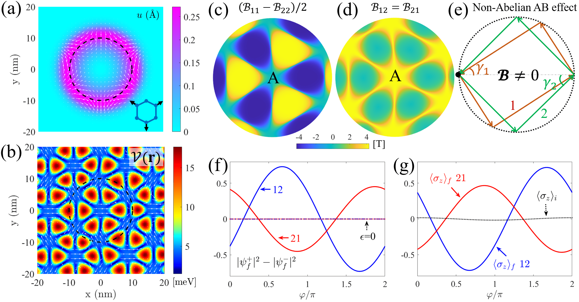
Figure 4: Non-Abelian gauge field and AB effect in triaxially strained R-type $2^{\circ}$ twisted bilayer MoSe₂. (a) Magnitude (background) and vector flow (arrows) of the strain displacement. Inset shows schematics of triaxial stress. (b) Distribution of $\mathcal{V}$ with arrows denoting the in-plane component of $\hat{\boldsymbol{\mathcal{V}}}$. (c) Diagonal and (d) off-diagonal components of the non-Abelian gauge field. Center of the strained area has the A stacking. (e) Schematics of non-Abelian AB effect setup with loop ordering $1\rightarrow 2$ or $2\rightarrow 1$. $\gamma_{1}=30^{\circ}$ and $\gamma_{2}=40^{\circ}$. (f) Population redistribution in the two internal states $\ket{\chi_{\pm}}$ vs $\varphi$ when the particle travels $1\rightarrow 2$ (solid blue) or $2\rightarrow 1$ (dashed red). (g) Population redistribution in the two layers $\braket{\sigma_{z}}$ at the starting/ending point [black dot in (e)] vs $\varphi$ after the particle travels the aforementioned paths. Black dotted curve shows $\braket{\sigma_{z}}$ for the initial state.

Initially on pseudospin $\ket{\psi_{i}}=\cos\eta\ket{\chi_{+}}+e^{i\varphi}\sin\eta\ket{\chi_{-}}$, we compare the final state $\ket{\psi_{f}}=\mathcal{P}\ket{\psi_{i}}=\psi_{f}^{+}\ket{\chi_{+}}+\psi_{f}^{-}\ket{\chi_{-}}$ after the electron travels two closed loops in the strained area in different orders [$1\rightarrow 2$ or $2\rightarrow 1$, Fig. 4(e)]. Fig. 4(f) plots $|\psi_{f}^{+}|^{2}-|\psi_{f}^{-}|^{2}$, as a function of the initial state phase angle $\varphi$, with $\eta=\pi/4$. The discrepancy between the two differently ordered paths is clearly seen, a signature of the genuine non-Abelian AB effect Goldman et al. (2014). Note that dynamical phase can also lead to a pseudospin precession, determined by the path integral of $\mathcal{\tilde{Z}_{\epsilon}}(\mathbf{r})$ and $\mathcal{V}(\mathbf{r})$. This, however, is expected to be loop-order independent and does not affect $|\psi_{f}^{+}|^{2}-|\psi_{f}^{-}|^{2}$.

We note that the $z$ component of the pseudospin corresponds to a measurable quantity, i.e. out-of-plane electrical polarization. Red and blue curves in Fig. 4(g) give the corresponding plots of the final state polarization $\braket{\sigma_{z}}$ for the evolutions in Fig. 4(f). The difference between the two differently ordered paths is also seen, both of which are distinct from the initial value (black dotted curve).

For comparison, we examine evolutions on the same pair of loops with different orders in the unstrained moiré, where the gauge field $\boldsymbol{\mathcal{B}}$ vanishes. These are shown by the dashed lines in Fig. 4(f). Although the SU(2) Berry connection $\boldsymbol{\mathcal{A}}_{\nabla}$ is finite and non-Abelian, it does not have any effect on $|\psi_{f}^{+}|^{2}-|\psi_{f}^{-}|^{2}$. Electrical polarization $\braket{\sigma_{z}}$ of the final states is also found to be identical to that of initial ones. Likewise, in decoupled bilayer, the strain induced pseudomagnetic field alone does not change $\braket{\sigma_{z}}$. In either scenarios, one can not distinguish the two loop orderings, $1\rightarrow 2$ vs $2\rightarrow 1$. The genuine non-Abelian AB effect signifies the profound role of the non-Abelian gauge field $\boldsymbol{\mathcal{B}}$, which arises from the interplay of inhomogeneous strain and interlayer coupling in the distorted moiré only.

While the conventional AB effect proves the physically measurable significance of gauge potential, its genuine non-Abelian version can be as fundamental in demonstrating the noncommutativity in non-Abelian gauge theory. Realization of the scenario in Fig. 4(e) relies on advances in nanoelectronics for manipulation of electron trajectory and readout of final pseudospin states. On the other hand, non-Abelian gauge field can have interesting manifestations in other transport phenomena. For instance, non-Abelian gauge fields are expected to generate distinct fractal patterns in the Hofstadter butterfly spectrum compared to their Abelian counterparts Yang et al. (2019), and whether integer quantum Hall effect is still observable in the non-Abelian regime also remains unresolved. Strained moiré superlattices can be an ideal arena for their exporations. Moreover, moiré superlattice has also proven to be a powerful experimental platform to explore quantum many-body phenomena, where the manifestation of noncommutativity of non-Abelian gauge field is also highly interesting Goldman et al. (2014).

I Acknowledgment

We thank Yusong Bai for providing the data of strained moiré structure and Qizhong Zhu for helpful discussions. The work is supported by the Research Grants Council of Hong Kong (Grants No. HKU17306819 and No. C7036-17W), and the University of Hong Kong (Seed Funding for Strategic Interdisciplinary Research).

References

- Cao et al. (2018a) Y. Cao, V. Fatemi, S. Fang, K. Watanabe, T. Taniguchi, E. Kaxiras, and P. Jarillo-Herrero, Nature 556, 43 (2018a).
- Cao et al. (2018b) Y. Cao, V. Fatemi, A. Demir, S. Fang, S. L. Tomarken, J. Y. Luo, J. D. Sanchez-Yamagishi, K. Watanabe, T. Taniguchi, E. Kaxiras, R. C. Ashoori, and P. Jarillo-Herrero, Nature 556, 80 (2018b).
- Sharpe et al. (2019) A. L. Sharpe, E. J. Fox, A. W. Barnard, J. Finney, K. Watanabe, T. Taniguchi, M. A. Kastner, and D. Goldhaber-Gordon, Science 365, 605 (2019).
- Yankowitz et al. (2019) M. Yankowitz, S. Chen, H. Polshyn, Y. Zhang, K. Watanabe, T. Taniguchi, D. Graf, A. F. Young, and C. R. Dean, Science 363, 1059 (2019).
- Serlin et al. (2020) M. Serlin, C. L. Tschirhart, H. Polshyn, Y. Zhang, J. Zhu, K. Watanabe, T. Taniguchi, L. Balents, and A. F. Young, Science 367, 900 (2020).
- Lu et al. (2019) X. Lu, P. Stepanov, W. Yang, M. Xie, M. A. Aamir, I. Das, C. Urgell, K. Watanabe, T. Taniguchi, G. Zhang, A. Bachtold, A. H. MacDonald, and D. K. Efetov, Nature 574, 653 (2019).
- Tang et al. (2020) Y. Tang, L. Li, T. Li, Y. Xu, S. Liu, K. Barmak, K. Watanabe, T. Taniguchi, A. H. MacDonald, J. Shan, and K. F. Mak, Nature 579, 353 (2020).
- Regan et al. (2020) E. C. Regan, D. Wang, C. Jin, M. I. Bakti Utama, B. Gao, X. Wei, S. Zhao, W. Zhao, Z. Zhang, K. Yumigeta, M. Blei, J. D. Carlström, K. Watanabe, T. Taniguchi, S. Tongay, M. Crommie, A. Zettl, and F. Wang, Nature 579, 359 (2020).
- Shimazaki et al. (2020) Y. Shimazaki, I. Schwartz, K. Watanabe, T. Taniguchi, M. Kroner, and A. Imamoğlu, Nature 580, 472 (2020).
- Yu et al. (2017) H. Yu, G.-B. Liu, J. Tang, X. Xu, and W. Yao, Sci. Adv. 3, e1701696 (2017).
- Seyler et al. (2019) K. L. Seyler, P. Rivera, H. Yu, N. P. Wilson, E. L. Ray, D. G. Mandrus, J. Yan, W. Yao, and X. Xu, Nature 567, 66 (2019).
- Tran et al. (2019) K. Tran, G. Moody, F. Wu, X. Lu, J. Choi, K. Kim, A. Rai, D. A. Sanchez, J. Quan, A. Singh, J. Embley, A. Zepeda, M. Campbell, T. Autry, T. Taniguchi, K. Watanabe, N. Lu, S. K. Banerjee, K. L. Silverman, S. Kim, E. Tutuc, L. Yang, A. H. MacDonald, and X. Li, Nature 567, 71 (2019).
- Jin et al. (2019) C. Jin, E. C. Regan, A. Yan, M. Iqbal Bakti Utama, D. Wang, S. Zhao, Y. Qin, S. Yang, Z. Zheng, S. Shi, K. Watanabe, T. Taniguchi, S. Tongay, A. Zettl, and F. Wang, Nature 567, 76 (2019).
- Alexeev et al. (2019) E. M. Alexeev, D. A. Ruiz-Tijerina, M. Danovich, M. J. Hamer, D. J. Terry, P. K. Nayak, S. Ahn, S. Pak, J. Lee, J. I. Sohn, M. R. Molas, M. Koperski, K. Watanabe, T. Taniguchi, K. S. Novoselov, R. V. Gorbachev, H. S. Shin, V. I. Fal’ko, and A. I. Tartakovskii, Nature 567, 81 (2019).
- Jauregui et al. (2019) L. A. Jauregui, A. Y. Joe, K. Pistunova, D. S. Wild, A. A. High, Y. Zhou, G. Scuri, K. De Greve, A. Sushko, C.-H. Yu, T. Taniguchi, K. Watanabe, D. J. Needleman, M. D. Lukin, H. Park, and P. Kim, Science 366, 870 (2019).
- Zhang et al. (2017) C. Zhang, C.-P. Chuu, X. Ren, M.-Y. Li, L.-J. Li, C. Jin, M.-Y. Chou, and C.-K. Shih, Sci. Adv. 3, e1601459 (2017).
- Wu et al. (2019) F. Wu, T. Lovorn, E. Tutuc, I. Martin, and A. H. MacDonald, Phys. Rev. Lett. 122, 086402 (2019).
- Yu et al. (2020) H. Yu, M. Chen, and W. Yao, Natl. Sci. Rev. 7, 12 (2020).
- Zhai and Yao (2020) D. Zhai and W. Yao, Phys. Rev. Materials 4, 094002 (2020).
- Bi et al. (2019) Z. Bi, N. F. Q. Yuan, and L. Fu, Phys. Rev. B 100, 035448 (2019).
- Wolf et al. (2019) T. M. R. Wolf, J. L. Lado, G. Blatter, and O. Zilberberg, Phys. Rev. Lett. 123, 096802 (2019).
- Liu et al. (2019) J. Liu, J. Liu, and X. Dai, Phys. Rev. B 99, 155415 (2019).
- San-Jose et al. (2012) P. San-Jose, J. González, and F. Guinea, Phys. Rev. Lett. 108, 216802 (2012).
- Wang et al. (2017) Y. Wang, Z. Wang, W. Yao, G.-B. Liu, and H. Yu, Phys. Rev. B 95, 115429 (2017).
- Goldman et al. (2014) N. Goldman, G. Juzeliūnas, P. Öhberg, and I. B. Spielman, Rep. Prog. Phys. 77, 126401 (2014).
- Yang et al. (2019) Y. Yang, C. Peng, D. Zhu, H. Buljan, J. D. Joannopoulos, B. Zhen, and M. Soljačić, Science 365, 1021 (2019).
- Bai et al. (2020) Y. Bai, L. Zhou, J. Wang, W. Wu, L. J. McGilly, D. Halbertal, C. F. B. Lo, F. Liu, J. Ardelean, P. Rivera, N. R. Finney, X.-C. Yang, D. N. Basov, W. Yao, X. Xu, J. Hone, A. N. Pasupathy, and X.-Y. Zhu, Nat. Mater. 19, 1068 (2020).
- van der Zande et al. (2014) A. M. van der Zande, J. Kunstmann, A. Chernikov, D. A. Chenet, Y. You, X. Zhang, P. Y. Huang, T. C. Berkelbach, L. Wang, F. Zhang, M. S. Hybertsen, D. A. Muller, D. R. Reichman, T. F. Heinz, and J. C. Hone, Nano Lett. 14, 3869 (2014).
- Amorim et al. (2016) B. Amorim, A. Cortijo, F. de Juan, A. Grushin, F. Guinea, A. Gutiérrez-Rubio, H. Ochoa, V. Parente, R. Roldán, P. San-Jose, J. Schiefele, M. Sturla, and M. Vozmediano, Phys. Rep. 617, 1 (2016).
- Tong et al. (2017) Q. Tong, H. Yu, Q. Zhu, Y. Wang, X. Xu, and W. Yao, Nat. Phys. 13, 356 (2017).
- Koshino and Nam (2020) M. Koshino and N. N. T. Nam, Phys. Rev. B 101, 195425 (2020).
- (32) See Supplemental Material, which includes discussions on extra effects of strain, details of moiré potential, extended figures, and Refs. Settnes et al. (2016); Enaldiev et al. (2020); de Juan et al. (2012); Yang (2015).
- Fang et al. (2018) S. Fang, S. Carr, M. A. Cazalilla, and E. Kaxiras, Phys. Rev. B 98, 075106 (2018).
- Xiao et al. (2012) D. Xiao, G.-B. Liu, W. Feng, X. Xu, and W. Yao, Phys. Rev. Lett. 108, 196802 (2012).
- Xiao et al. (2007) D. Xiao, W. Yao, and Q. Niu, Phys. Rev. Lett. 99, 236809 (2007).
- Aivazian et al. (2015) G. Aivazian, Z. Gong, A. M. Jones, R.-L. Chu, J. Yan, D. G. Mandrus, C. Zhang, D. Cobden, W. Yao, and X. Xu, Nat. Phys. 11, 148 (2015).
- Wu and Yang (1975) T. T. Wu and C. N. Yang, Phys. Rev. D 12, 3845 (1975).
- Xiao et al. (2010) D. Xiao, M.-C. Chang, and Q. Niu, Rev. Mod. Phys. 82, 1959 (2010).
- Mikael et al. (2017) S. Mikael, J.-H. Seo, D.-W. Park, M. Kim, H. Mi, A. Javadi, S. Gong, and Z. Ma, Extreme Mech. Lett. 11, 77 (2017).
- Nigge et al. (2019) P. Nigge, A. C. Qu, É. Lantagne-Hurtubise, E. Mårsell, S. Link, G. Tom, M. Zonno, M. Michiardi, M. Schneider, S. Zhdanovich, G. Levy, U. Starke, C. Gutiérrez, D. Bonn, S. A. Burke, M. Franz, and A. Damascelli, Sci. Adv. 5, eaaw5593 (2019).
- Jiang et al. (2017) Y. Jiang, J. Mao, J. Duan, X. Lai, K. Watanabe, T. Taniguchi, and E. Y. Andrei, Nano Lett. 17, 2839 (2017).
- Settnes et al. (2016) M. Settnes, S. R. Power, and A.-P. Jauho, Phys. Rev. B 93, 035456 (2016).
- Enaldiev et al. (2020) V. V. Enaldiev, V. Zólyomi, C. Yelgel, S. J. Magorrian, and V. I. Fal’ko, Phys. Rev. Lett. 124, 206101 (2020).
- de Juan et al. (2012) F. de Juan, M. Sturla, and M. A. H. Vozmediano, Phys. Rev. Lett. 108, 227205 (2012).
- Yang (2015) B. Yang, Phys. Rev. B 91, 241403(R) (2015).