Process monitoring based on orthogonal locality preserving projection with maximum likelihood estimation

Abstract

By integrating two powerful methods of density reduction and intrinsic dimensionality estimation, a new data-driven method, referred to as OLPP-MLE (orthogonal locality preserving projection-maximum likelihood estimation), is introduced for process monitoring. OLPP is utilized for dimensionality reduction, which provides better locality preserving power than locality preserving projection. Then, the MLE is adopted to estimate intrinsic dimensionality of OLPP. Within the proposed OLPP-MLE, two new static measures for fault detection $T_{\scriptscriptstyle{OLPP}}^{2}$ and ${\rm SPE}_{\scriptscriptstyle{OLPP}}$ are defined. In order to reduce algorithm complexity and ignore data distribution, kernel density estimation is employed to compute thresholds for fault diagnosis. The effectiveness of the proposed method is demonstrated by three case studies.

I Introduction

In recent decades, process monitoring becomes an increasingly significant and valuable research topic due to the high requirements of safety and reliability in industrial applications [1, 2, 3]. Specularly, data-driven process monitoring has attracted worldwide attention and has acquired remarkable accomplishments [4, 5, 7, 6]. The key contribution of data-driven techniques is to take advantage of sensing variables to detect faults, which makes them applicable in realistic industrial systems [8, 9, 10].In modern society, industrial systems such as power plants and high-speed rail become more complex, and produce massive data even in just one hour. Hence, how to extract valuable information from available data becomes the most critical issue at present.

There are various methods for data-driven process monitoring now. Classical schemes include principal component analysis (PCA) [11], partial least squares (PLS) [12, 13], independent component analysis (ICA) [14], canonical variate analysis [15], etc. Owing to simplicity and effectiveness in dealing with large data, PCA is recognized as a popular dimensionality reduction technique for linear systems, which has been widely applied to feature extraction as well as process monitoring areas [16, 17]. For instance, recursive total principle component regression was proposed for vehicular cyber-physical systems, which is able to detect small faults and suitable for on-line implementation [18]. There are also numerous fault detection methods based on PCA and PLS [13, 19], which have been integrated on the Matlab toolbox [20]. However, PCA aims to discover the global geometric topological structure of the Euclidean space, without considering the underlying local manifold structure.

Locality preserving projection (LPP) is regarded as an effective way to replace PCA, where local neighborhood framework of data could be optimally preserved [21, 22]. Based on LPP, orthogonal locality preserving projection (OLPP) was proposed to reconstruct data conveniently, where mutually orthogonal basis functions are calculated. Besides, OLPP can realize the function of PCA when the parameter is set appropriately and eigenvectors corresponding to largest eigenvalues are retained[23], which indicates that OLPP can not preserve global and local geometric structure simultaneously.

Note that OLPP shares several data representation characteristics with nonlinear techniques, for instance, Laplacian Eigenmaps (LE) [24], Isomap [25] and locally linear embedding [26, 27]. These local nonlinear manifold approaches are non-parametric without parametric hypothesis and are casted into the eigen-problem instead of iteration, which makes them considerably less complicated [28, 29]. However, “out of sample” issue severely constraints the applications of process monitoring. OLPP is exactly the linear extension of LE algorithm and can efficiently deal with this issue.

For the OLPP approach, the intrinsic dimensionality (ID) is the most critical parameter [30]. If the ID is too small, significant data characteristics may be “collapsed” onto the same dimension. However, if the ID is too large, the projections become noisy and may be unstable. Therefore, the estimation of the optimal ID is the prime task that should be considered. In this paper, as a local estimator of ID, maximum likelihood estimation (MLE) is adopted to calculate the ID with little artificial interference, which has the superiorities of easy-implementation, stability, high reliability [31, 32, 33]. Besides, it is also robust to noisy data and less computationally complicated on high dimensional data [34].

Since OLPP is a preferable choice for dimensionality reduction, an improved data-driven process monitoring approach is proposed based on OLPP, referred as to OLPP-MLE, where MLE is embedded in OLPP framework. Unfortunately, although the ID estimator is provided, OLPP still encounters the singular issue frequently, especially for data with zero mean. Within the proposed approach, the singular problem is efficiently settled with three optional solutions, which is the meaningful improvement compared with traditional OLPP. Besides, an alternative manner is provided to calculate eigenvector with little computational cost.

The virtues of the proposed OLPP-MLE are summarized as follows:

1. The proposed approach provides more locality preserving power and discriminating power than most typical dimensionality reduction approaches;

2. Because OLPP and MLE are based on local geometric characteristics of data, the proposed approach is considerably less computationally complicated in contrast with global approaches;

3. For the potential singular problem within the standard OLPP, three alternative solutions are summarized, which provides more choices for researchers to select;

4. MLE provides a stable estimation of the ID, which is insensitive to parameter tuning;

5. The proposed method has no requirement of data distribution, which is beneficial to expand its applications.

The remaining parts of this paper are organized below. Section II summarizes the preliminary of OLPP and MLE on intrinsic dimensionality briefly. Major procedure of OLPP-MLE approach is summarized for data-driven process monitoring in Section III. The solutions of singular problem, an alternative approach to calculate eigenvectors and computational complexity analysis are also discussed thereafter. Then, a numerical case study and the continuous stirred tank reactor (CSTR) are adopted to illustrate the effectiveness of the proposed approach in Section IV. Section V utilizes Tennessee Eastman (TE) process to verify the stability of the proposed approach and to compare with several typical data-driven approaches. Conclusion is presented in Section VI.

II Preliminaries

In this section, we introduce two independent important works on MLE of ID [31] and the algorithm of OLPP [22], which are both based on the local geometric properties of data. These works form the building stones of our proposed data-driven process monitoring algorithm.

II-A Maximum likelihood estimation on intrinsic dimensionality

The MLE of ID is derived by  Levina and Bickel [31]. Assume a data set ${\{\bm{x}_{i}\}_{i=1}^{N}\subset{\mathcal{R}^{m}}}$, representing an embedding of a lower-dimensional sample $\bm{x_{i}}=g(\bm{y_{i}})$, where $g(.)$ is a continuous and smooth mapping, and $\bm{y}_{i}$ are sampled from an unknown density $p$ on ${\mathcal{R}^{l}}$. For the purpose of ID estimation, it is initially assumed that $p\approx const$ in a small hyper sphere $H_{\bm{x}}(t)$ around a data point $\bm{x}$. The data points inside the hyper sphere are modelled as a Poisson process. Let the counts of the observations with distance $t$ from $\bm{x}$ be denoted as

$$C(t,\bm{x})=\sum_{i=1}^{N}1\{\bm{x}_{i}\in H_{\bm{x}}(t)\}$$ (1)

where $0\leq t\leq R$, $H_{\bm{x}}(t)$ is a small hyper sphere around a data point $\{\bm{x}\}$ with radius $t$. For fixed $N$, $C(t,\bm{x})$ is approximated as a Poisson process, and the rate of the process $\lambda\left(t\right)$ of the $C(t,\bm{x})$ is given by

$$\lambda\left(t\right)=p(\bm{x})V(l)l\cdot t^{l-1},$$ (2)

where $V(l)=\pi^{l/2}[\Gamma(l/2+1)]^{-1}$ denotes the volume of the unit sphere in ${\mathcal{R}^{l}}$. It can be shown that the log-likelihood of the observed $C(t,\bm{x})$ can be expressed as

$$\int_{0}^{R}\log\lambda(t)dC(t)-\int_{0}^{R}\lambda(t)dt,$$ (3)

The maximization of (3) results in a unique solution $l$. In practice, $l$ can be obtained based on a data point $\bm{x}_{i}$ given $k$ nearest neighbors, which is calculated by [31]

$${\mathop{l}\limits^{\wedge}}_{k}\left({{\bm{x}_{i}}}\right)={\left({\frac{1}{{k-1}}\sum\limits_{j=1}^{k-1}{\log\frac{{{F_{k}}\left({{\bm{x}_{i}}}\right)}}{{{F_{j}}\left({{\bm{x}_{i}}}\right)}}}}\right)^{-1}},$$ (4)

where ${{F_{k}}\left({{\bm{x}_{i}}}\right)}$ is the smallest radius of the hypersphere with center $\bm{x}_{i}$, which must contain $k$ neighboring data points.

It is obvious that $k$ affects the estimate severely. In general, the estimator is expected to be small enough and contain as many points as possible. In our approach, just average over a range of small to moderate values $k=k_{1},\ldots,k_{2}$ to obtain the optimal estimate

$${\widehat{l}_{k}}=\frac{1}{N}\sum\limits_{i=1}^{N}{{{\widehat{l}}_{k}}\left({{\bm{x}_{i}}}\right)},\quad\widehat{l}=\frac{1}{{{k_{2}}-{k_{1}}+1}}\sum\limits_{{k_{1}}}^{{k_{2}}}{{{\widehat{l}}_{k}}}.$$ (5)

The perfect range $k_{1},\ldots,k_{2}$ is different for every combination of $l$ and $N$, but the estimation of dimensionality is considerably stable, which has already been demonstrated [31]. Given $l$ and $N$, $l$ is not sensitive to $k_{1}$ and $k_{2}$, which is discussed in Section V-B. For simplicity and reproducibility, $k_{1}$ and $k_{2}$ are fixed in this paper.

II-B Orthogonal locality preserving projection

OLPP is a common dimensionality reduction approach, and can preserve the local geometric characteristics of the manifold [22]. Given a data set $\bm{X}=[{\bm{x}_{1}},....,{\bm{x}_{N}}]$ with $\bm{x}_{i}\in\mathcal{R}^{m},i=1,\cdots,N$. Let $\bm{S}$ be a similarity matrix defined on data points, which is computed by

$${\bm{S}_{ij}}={e^{-\frac{{{{\left\|{{\bm{x}_{i}}-{\bm{x}_{j}}}\right\|}^{2}}}}{q}}},$$ (6)

where $q$ is predefined by users. Define $\bm{D}$ as a diagonal matrix with ${{\bm{D}_{ii}}=\sum\limits_{j=1}^{N}{{\bm{S}_{ji}}}}$. Then, ${\bm{L}=\bm{D}-\bm{S}}$ is Laplacian matrix in graph theory. The objective function of OLPP can be written as

$$\{\bm{a}_{1},...,\bm{a}_{l}\}=\min_{\bm{a}}\{f(\bm{a})=\frac{{\bm{a}}^{\rm T}\bm{X}\bm{L}\bm{X}^{\rm T}{\bm{a}}}{{\bm{a}}^{\rm T}\bm{X}\bm{D}\bm{X}^{\rm T}{\bm{a}}}\}$$ (7)

subject to $\bm{a}_{i}^{\rm T}\bm{a}_{j}=0$, for $i\neq j$. The OLPP algorithm is presented concretely in Appendix. The OLPP aims at finding ${\left\{{{\bm{y}_{i}}}\right\}_{i=1}^{N}\in{\mathcal{R}^{l}},l\ll m}$, where $\bm{y}_{i}$ can “represent” $\bm{x}_{i}$, and $l$ is the ID of data. OLPP is applicable especially in the particular situation, where ${{\bm{x}_{1}},{\bm{x}_{2}},\cdots,{\bm{x}_{N}}\in{\bm{M}}}$ and $\bm{M}$ is a nonlinear manifold.

III OLPP-MLE for fault diagnosis

In this section, two well-known statistics $T^{2}$ and $\rm SPE$ [35], transitionally based on PCA or other variants [36, 11] are served as indices to monitor the operating process, referred to as $T_{\scriptscriptstyle{OLPP}}^{2}$ and ${\rm SPE}_{\scriptscriptstyle{OLPP}}$. As aforementioned, OLPP has more locality preserving power than most typical dimensionality reduction methods, which may lead to discriminating capability for data anomaly.

Consider that OLPP is applied based on a set of normal training samples ${\{\bm{x}_{i}\}_{i=1}^{N}\in{\mathcal{R}^{m}}}$ based on a given dimension $l$, which is obtained by MLE of the ID in Section II-A. Let ${{\bm{W}_{\scriptscriptstyle{OLPI}}}=\left[{{{\bm{a}}}_{1},\cdots,{{\bm{a}}}_{l}}\right]}$, with ${{\bm{W}_{\scriptscriptstyle{OLPI}}^{\rm T}}{\bm{W}_{\scriptscriptstyle{OLPI}}}={\bm{I}}}$. The resultant OLPI mapping becomes

$$\bm{x}\to\bm{y}={\bm{W}}_{\scriptscriptstyle{OLPI}}^{\rm T}{\bm{x}},$$ (8)

where $\bm{y}$ is an $l$-dimensional expression of raw $\bm{x}$. Denote ${\bm{Y}=[{\bm{y}_{1}},....,{\bm{y}_{N}}]}$.

$T_{\scriptscriptstyle{OLPP}}^{2}$ monitoring statistic for principal component subspace is calculated by

$${T_{\scriptscriptstyle{OLPP}}^{2}}={\bm{y}^{\rm T}}{\bm{\Lambda}^{-1}}{\bm{y}},$$ (9)

where the elements of ${\bm{\Lambda}=diag({\gamma_{1}},\ldots,{\gamma_{l}})}$ are the eigenvalues of the covariance matrix of $\bm{Y}$ with descending order ${{\gamma_{1}}\geq\ldots\geq{\gamma_{l}}>0}$. Then, ${\rm SPE}_{\scriptscriptstyle{OLPP}}$ is utilized to detect the abnormal change in the residual subspace and calculated as

${\rm SPE}_{\scriptscriptstyle{OLPP}}={\left\|{\bm{x}-\widehat{\bm{x}}}\right\|^{2}}$,

where $\bm{x}$ is preprocessed by data normalization and $\widehat{\bm{x}}$ is the reconstruction of $\bm{x}$. The system model based on OLPP is given as

${\bm{x}}=\widehat{\bm{x}}+{\bm{e}}={\bm{W}}_{\scriptscriptstyle{OLPI}}{\bm{y}}+{\bm{e}}$

for which (8) provides the optimal solution of minimizing $\|{\bm{e}}\|^{2}$, then we have $\widehat{\bm{x}}=\bm{W}_{\scriptscriptstyle{OLPI}}\bm{W}_{\scriptscriptstyle{OLPI}}^{\rm T}\bm{x}$.

$${\rm SPE}_{\scriptscriptstyle{OLPP}}= {{\bm{x}}}^{\rm T}\big{(}\bm{I}-\bm{W}_{\scriptscriptstyle{OLPI}}\bm{W}^{\rm T}_{\scriptscriptstyle{OLPI}}\big{)}^{2}{{\bm{x}}}$$

$$= {{\bm{x}}}^{\rm T}\big{(}\bm{I}-\bm{W}_{\scriptscriptstyle{OLPI}}\bm{W}^{\rm T}_{\scriptscriptstyle{OLPI}}\big{)}{{\bm{x}}}$$

$$= \left\|\bm{x}\right\|^{2}-\left\|\bm{y}\right\|^{2}$$ (10)

by making use of ${\bm{W}_{\scriptscriptstyle{OLPI}}^{\rm T}}{\bm{W}_{\scriptscriptstyle{OLPI}}}={\bm{I}}$.

For OLPP-MLE, our proposed $T_{\scriptscriptstyle{OLPP}}^{2}$ and ${\rm SPE}_{\scriptscriptstyle{OLPP}}$ serve as significant indices to monitor the process, and the associated thresholds provide the reference to judge whether faults occur or not. Because the proposed OLPP-MLE is free from data distribution, kernel density estimation (KDE) technique is adopted to calculate thresholds, which is presented concisely below [15].

Given a random variable $z$, $p(z)$ is the associated probability density function, then

$$\mathop{p}\limits^{\wedge}(z)=\frac{1}{{N\kappa}}\sum\limits_{n=1}^{N}{\psi(\frac{{z-{z_{n}}}}{\kappa})},$$ (11)

where ${{z_{n}}(n=1,\ldots,N)}$ can represent ${T_{\scriptscriptstyle{OLPP}}^{2}}$ and ${\rm SPE}_{\scriptscriptstyle{OLPP}}$ statistics aforementioned. $\kappa$ is the bandwidth of kernel function $\psi\left(\cdot\right)$, which influences the estimation of $p(z)$ seriously. In this paper, the optimal value $\kappa_{opt}$ is calculated by the following criterion, where $\sigma$ is standard deviation [15]:

$${\kappa_{opt}}=1.06\sigma{N^{-1/5}}.$$ (12)

Given a confidence limit $\alpha$, the thresholds $J_{th,T^{2}}$ and $J_{th,{\rm SPE}}$ are computed by

$$\int_{-\infty}^{{J_{th,T^{2}}}}{\mathop{p}\limits^{\wedge}(T_{{\scriptscriptstyle{OLPP}}}^{2})d}{T_{\scriptscriptstyle{OLPP}}^{2}}=\alpha,$$ (13)

$$\int_{-\infty}^{{J_{th,{\rm SPE}}}}{\mathop{p}\limits^{\wedge}({\rm SPE}_{\scriptscriptstyle{OLPP}})d}{{\rm SPE}_{\scriptscriptstyle{OLPP}}}=\alpha$$ (14)

III-A Summary of the proposed approach

The main procedure of OLPP-MLE fault diagnosis algorithm can be summarized thereafter.

The off-line modeling phase is depicted as follows.

1. Data normalization. Calculate the mean and standard deviation of the history data, which are normalized to zero mean and scaled to unit variance.

2. Estimate the ID of data via (4-5).

3. Calculate the orthogonal locality preserving projections ${\bm{W}_{\scriptscriptstyle{OLPI}}}$ according to SI file.

4. Obtain the lower-dimensional representation y by (8).

5. Calculate the monitoring statistics $T_{\scriptscriptstyle{OLPP}}^{2}$ and ${{\rm SPE}_{\scriptscriptstyle{OLPP}}}$ according to (9-III).

6. Calculate the thresholds corresponding to the statistics aforementioned by KDE technique, described by (11-14).

The on-line monitoring phase is presented below.

1. Collect and preprocess data. According to the mean and standard deviation in the off-line modeling phase, preprocess the collected testing data.

2. Calculate the lower-dimensional representation of new data via (8).

3. Calculate two monitoring statistics $T_{\scriptscriptstyle{OLPP}}^{2}$ and ${{\rm SPE}_{\scriptscriptstyle{OLPP}}}$ of new data according to (9-III).

4. Judge whether a fault happens based on the fault detection logic:

   ${\rm SPE}_{\scriptscriptstyle{OLPP}}\leq{J_{th,\rm SPE}}$ and $T_{\scriptscriptstyle{OLPP}}^{2}\leq{J_{th,T^{2}}}$ $\Rightarrow$ fault free, otherwise faulty.

Two indices are generally utilized to evaluate the algorithm accuracy, namely, fault detection rate (FDR) and false alarm rate (FAR), which could be calculated below.

$$\rm{FDR}=\frac{{number\;of\;samples\,\left({\emph{J}>{\emph{J}_{\emph{th}}}|\emph{f}\neq 0}\right)}}{{total\;samples\,\left({\emph{f}\neq 0}\right)}}\times 100\%$$ (15)

$$\rm{FAR}=\frac{{number\;of\;samples\,\left({\emph{J}>{\emph{J}_{\emph{th}}}|\emph{f}=0}\right)}}{{total\;samples\,\left({\emph{f}=0}\right)}}\times 100\%$$ (16)

where $J$ can be replaced by $T_{\scriptscriptstyle{OLPP}}^{2}$ or ${{\rm SPE}_{\scriptscriptstyle{OLPP}}}$, and $J_{th}$ is the associated threshold.

III-B Remarks

• Solutions of singular matrix $\bm{X}\bm{D}\bm{X}^{\rm T}$

  For the crucial step of calculating OLPP, matrix ${(\bm{X}\bm{D}\bm{X}^{\rm T})^{-1}}$ is considerably critical. However, $\bm{X}\bm{D}\bm{X}^{\rm T}$ is singular in most cases, especially when $\bm{X}$ has data redundancy or is normalized to zero mean. Thus, the inverse matrix $(\bm{X}\bm{D}\bm{X}^{\rm T})^{-1}$ does not actually exist. In our approach, three alternative methods are provided to cope with this issue.

  1) PCA projection

  Before conventional OLPP, $\bm{x}$ is firstly projected into PCA subspace and then irrelevant features are extracted. Let $\bm{W}_{\scriptscriptstyle{PCA}}$ denote the transformation matrix via PCA and $\widehat{\bm{X}}$ denote the reconstruction of $\bm{X}$ after PCA projection. As the preprocessing step of OLPP, it ensures that matrix ${\widehat{\bm{X}}{\bm{D}}\widehat{\bm{X}}^{\rm T}}$ is nonsingular. In the following procedure, ${\bm{X}}$ is replaced by $\widehat{\bm{X}}$ accordingly. At the fourth step of OLPP in SI file, the transformation matrix $\bm{W}$ is calculated by

  $$\bm{W}=\bm{W}_{\scriptscriptstyle{PCA}}{\bm{W}_{\scriptscriptstyle{OLPI}}}.$$ (17)

  Since vectors in $\bm{W}_{\scriptscriptstyle{PCA}}$ and $\bm{W}_{\scriptscriptstyle{OLPI}}$ are orthonormal, vectors in $\bm{W}$ are still mutually orthonormal. Hence, $\bm{W}$ should be substituted for $\bm{W}_{\scriptscriptstyle{OLPI}}$ in (8), and the rest procedure remains the same.

  2) Regularization

  Regularization is a common technique to cope with singular problem. In the proposed approach, the regularization term is utilized by adding constant values to the diagonal elements of ${\bm{X}\bm{D}\bm{X}^{\rm T}}$, as ${{\bm{X}\bm{D}\bm{X}^{\rm T}}+\beta\bm{I}}$, where $\beta>0$ is predefined by users. It is obviously that ${\bm{X}\bm{D}\bm{X}^{\rm T}+\beta\bm{I}}$ is non-singular.

  3) Pseudo inverse

  When ${\bm{X}\bm{D}\bm{X}^{\rm T}}$ is singular, the concept of pseudo inverse is introduced, which denotes as $(\cdot)^{\dagger}$. Suppose ${rank(\bm{X}\bm{D}\bm{X}^{\rm T})=r}$, the singular value decomposition (SVD) of this matrix is

  $$\bm{X}\bm{D}\bm{X}^{\rm T}=\bm{P}{\bm{\Sigma}}{\bm{Q}^{\rm T}},$$ (18)

  where ${{\bm{\Sigma}}\in{\mathcal{R}}^{r\times r}}$, ${{\bm{P},\bm{Q}}\in{\mathcal{R}}^{N\times r}}$, $\bm{P}^{\rm T}{\bm{P}}=\bm{Q}^{\rm T}{\bm{Q}}=\bm{I}$. Then, pseudo inverse of matrix ${\bm{X}\bm{D}\bm{X}^{\rm T}}$ can be computed by

  $${\left({\bm{X}\bm{D}\bm{X}^{\rm T}}\right)^{\dagger}}=\bm{Q}{\bm{\Sigma}^{-1}}{\bm{P}^{\rm T}}.$$ (19)

  Thus, ${\left({\bm{X}\bm{D}\bm{X}^{\rm T}}\right)^{\dagger}}$ is substituted for ${\left({\bm{X}\bm{D}\bm{X}^{\rm T}}\right)^{-1}}$ in the following derivation process.

• Another perspective to calculate vector $\bm{a}_{1}$

  With regard to vector $\bm{a}_{1}$, it is the eigen-vector of $\bm{X}\bm{L}\bm{X}^{\rm T}\bm{a}=\lambda\bm{X}\bm{D}\bm{X}^{\rm T}\bm{a}$ corresponding to the smallest eigenvalue. Three alternative solutions aforementioned are fairly effective when $\bm{X}\bm{D}\bm{X}^{\rm T}$ is singular. Besides, SVD approach can also be widely employed to settle the underlying singular problem [37].

  Suppose $rank(\bm{X})=r_{x}$, the SVD of $\bm{X}$ is

  $$\bm{X}=\bm{U}{\bm{\Sigma}_{x}}{\bm{V}^{\rm T}}$$ (20)

  where ${{\bm{\Sigma}_{x}}\in{\mathcal{R}}^{r_{x}\times r_{x}}}$, ${\bm{U},\bm{V}\in{\mathcal{R}^{N\times{r_{x}}}}}$ and ${\bm{U}^{\rm T}}{\bm{U}}={\bm{V}^{\rm T}}{\bm{V}}=\bm{I}$. Let $\bm{b}=\bm{\Sigma}_{x}{\bm{U}^{\rm T}}{\bm{a}}$, then

  $$\bm{X}\bm{L}{\bm{X}^{\rm T}}\bm{a}=\lambda\bm{X}\bm{D}{\bm{X}^{T}}\bm{a}$$ (21)

  $$\Rightarrow \bm{U}\bm{\Sigma}_{x}{\bm{V}^{\rm T}}\bm{L}\bm{V}\bm{\Sigma}_{x}{\bm{U}^{\rm T}}\bm{a}=\lambda\bm{U}\bm{\Sigma}_{x}{\bm{V}^{\rm T}}\bm{D}\bm{V}\bm{\Sigma}_{x}{\bm{U}^{\rm T}}\bm{a}$$

  $$\Rightarrow \bm{U}\bm{\Sigma}_{x}{\bm{V}^{\rm T}}\bm{L}\bm{V}\bm{b}=\lambda\bm{U}\bm{\Sigma}_{x}{\bm{V}^{\rm T}}\bm{D}\bm{V}\bm{b}$$

  $$\Rightarrow {\bm{\Sigma}_{x}^{-1}}{\bm{U}^{\rm T}}\bm{U}\bm{\Sigma}_{x}{\bm{V}^{\rm T}}\bm{L}\bm{V}\bm{b}=\lambda{\bm{\Sigma}_{x}^{-1}}{\bm{U}^{\rm T}}\bm{U}\bm{\Sigma}_{x}{\bm{V}^{\rm T}}\bm{D}\bm{V}\bm{b}$$

  $$\Rightarrow {\bm{V}^{\rm T}}\bm{L}\bm{V}\bm{b}=\lambda{\bm{V}^{\rm T}}\bm{D}\bm{V}\bm{b}.$$

  It is obvious that $\bm{V}^{\rm T}\bm{D}\bm{V}$ is nonsingular and the generalized eigen-problem in (21) can be easily obtained. After $\bm{b}^{*}$ is obtained, $\bm{a}^{*}$ is computed by

  $$\bm{a}^{*}=\bm{U}{\bm{\Sigma}_{x}^{-1}}\bm{b}^{*}.$$ (22)

• Computational complexity analysis: According to the procedure of OLPP-MLE, the computation mainly contains adjacency graph construction, embedding functions and the estimation of ID via MLE. Since the computational complexity of $k$-nearest neighbor (KNN) is $O(N)$, thus the computational complexity of adjacency graph construction and MLE is also $O(N)$, which both obtain excellent relevant results based on KNN. The embedding functions needs $l$ times SVD on $m\times m$ matrix and $4(l-1)$ times matrix inversion on $m\times m$ matrix.

IV Numerical case and CSTR case studies

IV-A Numerical example

Considering the following system

$\left\{\begin{array}[]{l}{x_{1}}=t+{\varepsilon_{1}}\\ {x_{2}}=\cos t+{\varepsilon_{2}}\\ {x_{3}}={t^{2}}+t+{\varepsilon_{3}}\end{array}\right.,$

where ${t\in[-1,1]}$ and noise term ${\varepsilon_{i}(i=1,2,3)}$ follow uniform distribution with ${\varepsilon_{i}}\in[-0.05,0.05]$.

$1000$ normal samples are generated to train the process monitoring model and then artificial faults are generated with $1000$ samples by the following scheme:

1) Fault $1$: variable $x_{1}$ is added by 0.6 from the $501$th sample;

2) Fault $2$: variable $x_{2}$ is added by 0.8 from the $501$th sample;

3) Fault $3$: variable $x_{3}$ is added by 1.0 from the $501$th sample.

Note that $T_{\scriptscriptstyle{OLPP}}^{2}$ and ${{\rm SPE}_{\scriptscriptstyle{OLPP}}}$ are recorded briefly as $T^{2}$ and SPE in simulation figures for simplicity and convenience.

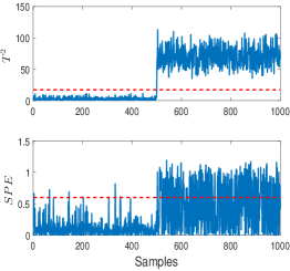
(a) Fault 1

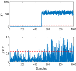
(b) Fault 2

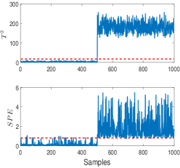
(c) Fault 3

Figure 1: Monitoring charts of numerical case

Monitoring consequences are illustrated in Figure 1. The FDRs of three faults nearly approach to $100\%$ and the FARs are all below $5\%$. Specifically, with regard to Faults $1$ and $2$, $T^{2}$ monitoring statistic can totally detect the fault while SPE has several missed alarm points. As illustrated in Figure 1(c), both monitoring statistics can detect Fault $3$ timely and accurately. In conclusion, faults can be detected by the cooperation of $T^{2}$ and SPE monitoring statistics, which indicates that OLPP-MLE is able to monitor this process.

IV-B Case study on CSTR

In this section, we employ MLE to estimate the ID, then PCA, LPP and OLPP are adopted to monitor the process. Thus, PCA-MLE, LPP-MLE and OLPP-MLE are compared and the superiority of OLPP-MLE is illustrated by CSTR.

IV-B1 CSTR introduction

The dynamic behavior of CSTR process is depicted as follows [38]:

$$\frac{{d{C_{A}}}}{{dt}}=\frac{q}{V}\left({{C_{Af}}-{C_{A}}}\right)-{k_{0}}\exp\left\{{-\frac{E}{{RT}}}\right\}{C_{A}}+{v_{1}}$$ (23)

$$\frac{{dT}}{{dt}}=\frac{q}{V}\left({{T_{f}}-T}\right)-\frac{{\Delta H}}{{\rho{C_{p}}}}{k_{0}}\exp\left\{{-\frac{E}{{RT}}}\right\}{C_{A}}+\frac{{UA}}{{V\rho{C_{p}}}}\left({{T_{c}}-T}\right)+{v_{2}}$$ (24)

where the outlet concentration $C_{A}$ and the outlet temperature $T$ are controlled by PI controllers, $q$ is the feed flow rate, $C_{Af}$ is the feed concentration, $V$ is the volume of the vessel, $T_{f}$ is the feed temperature, $v_{1}$ and $v_{2}$ are independent system noises [39].

In this simulation, the sampling interval is 1 second. The measured process variable $\left[{{C_{A}}\,\;T\,\;{T_{c}}\,\;q}\right]\;$ are collected, and the measurement noise $e$ is added. Besides, negative feedback inputs were added to $\left[{\;q\,\;{T_{c}}}\right]\;$ with PID controllers as ${\bm{K}_{2}}\left({{K_{1}}+{{{T_{d}}s+{T_{I}}}\mathord{\left/{\vphantom{{{T_{d}}s+{T_{I}}}s}}\right.\kern-1.2pt}s}}\right)\varepsilon$, where $\varepsilon=[{C_{Af}}-C_{A}^{*},T-{T^{*}}]$ is the residual vector. All system parameters and conditions are set as the same with Li et al [40].

IV-B2 Monitoring results of CSTR case

In this paper, 6000 normal samples are collected to establish the monitoring model, that is, PCA-MLE, LPP-MLE and OLPP-MLE. We collect samples of 600 minutes and the faults are designed as follows:

1) Fault 4: the feed temperature $T_{f}$ is increased by $1\%$ at the 101th min;

2) Fault 5: the volume of vessel $V$ is decreased at the rate of $\frac{{\rm{4}}}{{{\rm{500}}}}$ $m^{3}$/mins.

In this simulation, the raw data is preprocessed by a low pass filter to reduce noise. Then, PCA-MLE, LPP-MLE and OLPP-MLE are adopted to monitor the process. The intrinsic dimensionality is 4 through MLE technique. Thus, only $T^{2}$ monitoring statistic works. As exhibited in Figures 2 and 3, it reveals that outlines of monitoring charts are similar for different approaches. The monitoring results are summarized in Table I. It shows that the FDRs of the proposed OLPP-MLE approach are the highest, especially for Fault 5. Moreover, the FARs are lower than $1\%$.

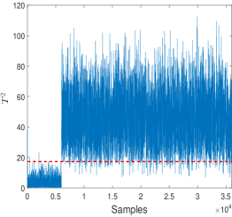
(a) PCA-MLE

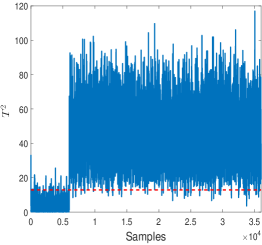
(b) LPP-MLE

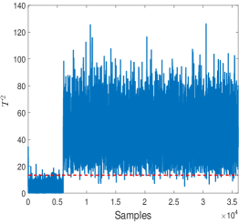
(c) OLPP-MLE

Figure 2: Monitoring charts of Fault 4

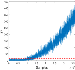
(a) PCA-MLE

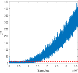
(b) LPP-MLE

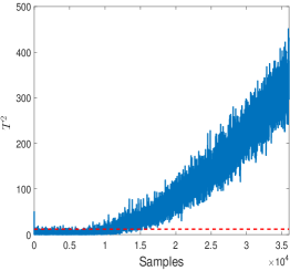
(c) OLPP-MLE

Figure 3: Monitoring charts of Fault 5

TABLE I: FDRs (%) and FARs (%) of CSTR case

Fault type	PCA-MLE	LPP-MLE	OLPP-MLE
Normal operation	0.13	0.57	0.50
Fault 4	98.98	99.70	99.80
Fault 5	78.85	82.20	83.19

V Benchmark simulation and comparative study

In this section, Tennessee Eastman process data is employed to prove the proposed approach. Besides, several existing data-driven approaches are utilized to compare with OLPP-MLE.

V-A Tennessee Eastman process

TE process is a well-established simulator that is generally served as a preferred benchmark for fault detection research [13, 11, 4]. The flow diagram is shown in Figure 4 and more detailed information can be found in Down et al [41].

$20$ process faults and another valve fault were defined, namely, IDV(1)-IDV(21). IDV(0) represents normal operation condition. The types of faults include step, random variation, show drift, sticking, constant position and unknown faults [11]. Due to the frequent absence of sufficient process knowledge, it is necessary to employ data-driven techniques for process monitoring.

In this simulation, $22$ process variables and $11$ manipulated variables are selected as the samples. $960$ normal samples are used to establish the off-line model. Then, $960$ testing samples, including the first $160$ normal samples and the following $800$ faulty samples, are utilized to evaluate the algorithm. Let $\alpha=0.99$ be the confidence level.

Figure 4: The flow diagram of TE process

V-B Intrinsic dimensionality

In this section, the parameter of MLE and the sampling frequency are discussed when the ID is estimated. The influence of the range $k_{1},\ldots,k_{2}$ is illustrated in Figure 5(a), where $k_{1}\in\left[{1,30}\right]$ and $k_{2}\in\left[{k_{1}+1,33}\right]$. The ID remains the same, which indicates that the estimation of ID is insensitive to the range of $k_{1}$, $k_{2}$.

Figure 5(b) demonstrates the influence of sampling frequency. As we have 960 normal data in total, every $j$ interval, samples are taken to acquire the ID. It denotes that the sampling frequency reduces to $1/j$ with $j\in\left[{1,12}\right]$. It can be discovered evidently that the ID keeps basically constant in Figure 5(b). In summary, the estimation of ID is stable via MLE.

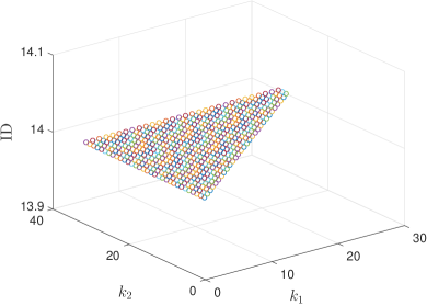
(a) The range of $k$

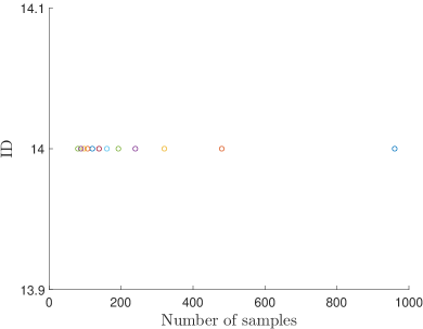
(b) Sampling frequency

Figure 5: The stability of estimating ID

V-C Simulation results of OLPP-MLE

Three typical faults, i.e., step, random variation and sticking, are selected to demonstrate OLPP-MLE algorithm. Specifically, fault IDV(1) is utilized to illustrate the step fault, fault IDV(12) is used to account for random variation fault, and fault IDV(14) is employed to represent the sticking fault.

In this simulation case, the ID is $14$ via MLE. Regularization is selected to figure out the underlying singular problem. The monitoring consequences of three typical faults are demonstrated in Figure 6. It can be obviously obtained that three faults can be detected timely and accurately. The FAR of OLPP-MLE is $0.63\%$, nearly close to $0$. The FDRs of fault IDV(1), fault IDV(12) and fault IDV(14), are $99.75\%$, $99.88\%$ and $100\%$, respectively. More specifically, two monitoring statistics can both detect these faults.

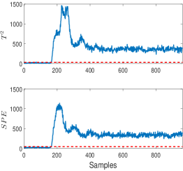
(a) IDV1

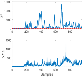
(b) IDV12

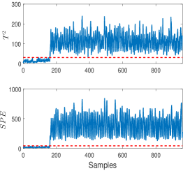
(c) IDV14

Figure 6: Monitoring charts of typical TE faults

V-D Comparative study with other techniques

In this section, PCA, dynamic PCA (DPCA) [42], probabilistic PCA (PPCA) [43], modified ICA (mICA) [14], LPP, traditional OLPP and the proposed OLPP-MLE are discussed.

TE data is employed to demonstrate the superiority of OLPP-MLE among the approaches aforementioned. For standard LPP and OLPP, nearest neighbor dimension estimator is employed to obtain the ID and its value is 3. For mICA, the ID is 9 based on leave-one-out cross validation. Eigenvalue-based estimator is adopted for PCA, and the number of principal components (PCs) is 9. Regarding DPCA, the time lag is 2 and 28 PCs are extracted via cumulative percent variance.

TABLE II: FDRs(% ) and FARs(%) based on TE data

Fault	PCA	DPCA	PPCA	mICA	LPP	OLPP	proposed
IDV(1)	99.88	99.75	99.75	98.88	99.75	99.50	99.75
IDV(2)	98.38	98.50	98.38	98.00	98.75	98.50	98.75
IDV(3)	4.50	3.25	2.13	2.25	9.25	11.75	13.75
IDV(4)	100	99.75	93.63	72.50	91.75	94.25	99.12
IDV(5)	100	99.75	25.37	99.75	99.75	100	100
IDV(6)	100	99.75	100	100	100	100	100
IDV(7)	100	99.75	100	100	96.75	100	100
IDV(8)	98.00	98.12	97.62	96.63	98.00	98.25	98.25
IDV(9)	3.50	3.88	1.87	3.25	6.50	10.00	12.50
IDV(10)	90.38	94.25	33.37	86.88	80.00	86.88	91.25
IDV(11)	80.63	93.00	62.50	56.25	67.87	72.50	87.35
IDV(12)	99.88	99.75	98.62	99.38	99.88	99.62	99.88
IDV(13)	95.25	96.00	94.25	95.13	94.63	95.75	96.13
IDV(14)	100	99.75	100	99.88	100	100	100
IDV(15)	7.00	15.75	1.75	2.38	11.75	12.25	21.13
IDV(16)	92.37	95.37	16.73	83.88	88.00	84.88	89.50
IDV(17)	97.25	97.88	88.62	89.25	90.25	89.50	93.63
IDV(18)	90.38	90.63	89.88	90.00	90.00	90.13	93.37
IDV(19)	94.63	99.62	20.13	52.25	74.75	82.37	91.00
IDV(20)	91.01	91.01	41.13	75.50	81.87	86.88	89.38
IDV(21)	57.75	52.25	40.50	53.63	45.12	48.38	58.37
IDV(0)	2.19	3.13	2.19	1.67	5.37	2.5	0.63

TABLE III: A brief comparison among data-driven approaches

Method	Assumption on data	Computational complexity	Parameter
PCA	Gaussian distribution	Low: 1 SVD on ${m\times m}$ matrix	number of PCs
DPCA	Same as PCA	Medium: 1 SVD on ${hm\times hm}$ matrix	number of PCs, $h$
PPCA	Same as PCA	High: key parameters determined by iterative EM	number of PCs
mICA	Non-Gaussian distribution	High: cost of PCA + iterative optimization issue	number of ICs
LPP	No	Low: cost of PCA + adjacency graph construction	$k$, $l$
OLPP	No	Medium: as mentioned in Section III-B	$k$, $l$
OLPP-MLE	No	Medium: as mentioned in Section III-B	$k$

The FARs and FDRs of these data-driven approaches are summarized in Table II. Among three manifold learning approaches, the proposed OLPP-MLE provides the optimal process monitoring performance including higher FDRs. It can be obviously discovered that the FAR of the proposed OLPP-MLE is the lowest. OLPP-MLE algorithm dramatically outperforms others, especially for IDV(3), IDV(9), IDV(15) and IDV(21), although all of the approaches can not detect faults accurately. For other faults except IDV(19), OLPP-MLE method provides the similar or sightly better fault detection performance in comparison with the other methods.

In conclusion, from overall perspective, OLPP-MLE has the highest detection accuracy rates after the trade-off between FAR and FDRs.

V-E Discussion on data-driven approaches

This section discusses the unsupervised dimensionality reduction approaches aforementioned in several aspects, namely, basic theory, mutual relationship, data distribution, computational complexity.

PCA can extract variability information to the utmost extent, but it should follow multivariate Gaussian distribution. DPCA has the most identical procedures with PCA and time delayed vectors are considered within, which makes it considerably complicated and not appropriate for large-scale systems. PPCA was proposed based on probabilistic model, where expectation maximization (EM) is employed to estimate the principal subspace iteratively. PPCA is able to deal with missing data but it is substantially complicated [44].

mICA extracts the latent statistically independent components (ICs) from non-Gaussian distribution data and can be regarded as another form of PCA [14]. However, the computational complexity of mICA is fairly high due to the iterative optimization issue.

Methods aforementioned are based on the global geometric properties of data. LPP can preserve local neighborhood message optimally. However, OLPP preserves better locality performance than LPP and enables to reconstruct data conveniently. Moreover, OLPP can be regarded as another form of PCA through the specific setting[23], which has been illustrated in SI file. OLPP-MLE can obtain accurate estimation of ID than traditional OLPP, thus delivering better monitoring performance, as indicated in Table II. OLPP-MLE is slightly more complicated than LPP and OLPP due to MLE. Other various virtues of the proposed method have been concluded in Section I.

A sketchy comparison among data-driven approaches aforementioned is summarized in Table III. According to Table III, OLPP-MLE has no requirement of data distribution, and the computational complexity is moderate and acceptable. Moreover, the estimation of ID is relatively accurate and stable, thus delivering better process monitoring performance than LPP and conventional OLPP. Therefore, OLPP-MLE is a preferable choice after thorough consideration.

VI Conclusion

In this paper a new process monitoring approach, i.e., OLPP-MLE, has been introduced based on available sensing measurements. The MLE is employed to estimate the intrinsic dimensionality of normal training data set, based on which OLPP is conducted to reduce dimensionality. Two test statistics are defined to monitor the model subspace and the residual subspace, and the corresponding thresholds are obtained by kernel density estimation. To deal with the singular problem in OLPP, three schemes are available to ensure the reliability of solution. Moreover, MLE provides stable and reliable estimation of intrinsic dimensionality. Besides, the proposed OLPP-MLE algorithm owns more discriminating capabilities for data anomaly, which may be otherwise indistinguishable via other dimensionality reduction methods. The superiority of OLPP-MLE is demonstrated by CSTR and Tennessee Eastman process in contrast with a wide range of data-driven fault detection schemes.

Actually, OLPP-MLE is based on the linear extension of Laplacian Eigenmaps and easy to reconstruct data, which shares several data representation characteristics with nonlinear techniques. In future, authors will focus on the nonlinear extension of OLPP-MLE with little artificial interference for the purpose of data-driven process monitoring. Besides, missing data and sparse data can also be considered.

Acknowledgment

This work was supported by the National Natural Science Foundation of China (61751307, 61490701, 61473164 and 61873143) and Research Fund for the Taishan Scholar Project of Shandong Province of China.

Appendix A OLPP algorithm

Algorithm of OLPP consists of following essential steps as below [22].

Step 1: Establish the adjacency graph

Let $G$ represent a graph with $N$ nodes. Then, the adjacency graph is established via $k$-nearest neighbor, which can be utilized to evaluate whether an edge should be put between two nodes [30].

Step 2: Calculate the weights $\bm{S}$

${\bm{S}\in{\mathcal{R}^{N\times N}}}$ is a similarity matrix and obviously sparse, where $\bm{S}_{ij}$ measures the similarity between $\bm{x}_{i}$ and $\bm{x}_{j}$.

Step 3: Calculate the orthogonal locality preserving projections

The orthogonal locality preserving projections are represented by ${\left\{{{\bm{a}_{1}},\cdots,{\bm{a}_{k}}}\right\}}$ and are calculated below.

$${\bm{A}^{\left({k-1}\right)}}=\left[{{\bm{a}_{1}},\cdots,{\bm{a}_{k}}}\right]$$ (25)

$${\bm{B}^{\left({k-1}\right)}}={\left[{{\bm{A}^{\left({k-1}\right)}}}\right]^{\rm T}}{\left({{\bm{X}}{\bm{D}}{\bm{X}^{\rm T}}}\right)^{-1}}{\bm{A}^{\left({k-1}\right)}}$$ (26)

The vectors ${\left\{{{\bm{a}_{1}},\cdots,{\bm{a}_{k}}}\right\}}$ can be calculated iteratively thereinafter:

$\bullet$ Calculate $\bm{a}_{1}$ as the eigenvector of ${{\left({{\bm{X}}{\bm{D}}{\bm{X}^{\rm T}}}\right)^{-1}}{\bm{X}}{\bm{L}}{\bm{X}^{\rm T}}}$ corresponding to the smallest eigenvalue.

$\bullet$ Calculate $\bm{a}_{k}$ as the eigenvector of the following matrix

$$\begin{array}[]{l}{\bm{M}^{\left(k\right)}}=\left\{{\bm{I}-{{\left({{\bm{X}}{\bm{D}}{\bm{X}^{\rm T}}}\right)}^{-1}}{\bm{A}^{\left({k-1}\right)}}{{\left[{{\bm{B}^{\left({k-1}\right)}}}\right]}^{-1}}}\right.\\ \quad\quad\;\;\,\;\;\;\left.{{{\left[{{\bm{A}^{\left({k-1}\right)}}}\right]}^{\rm T}}}\right\}\cdot{\left({{\bm{X}}{\bm{D}}{\bm{X}^{\rm T}}}\right)^{-1}}{\bm{X}}{\bm{L}}{\bm{X}^{\rm T}}\end{array}$$ (27)

corresponding to the smallest eigenvalue of ${\bm{M}^{\left(k\right)}}$.

Step 4: Orthogonal locality preserving index embedding

Let ${\bm{W}_{\scriptscriptstyle{OLPI}}}=\left[{\bm{a}}_{1},\cdots,{\bm{a}}_{l}\right]$, then data ${\bm{x}}$ can be mapped as

$$\bm{x}\to\bm{y}={\bm{W}^{\rm T}_{\scriptscriptstyle{OLPI}}}{\bm{x}},$$ (28)

where $\bm{y}$ is an $l$-dimensional expression of raw $\bm{x}$.

A-A Relationship between OLPP and PCA[23]

According to  He et al., $\bm{X}\bm{L}\bm{X}^{\rm T}$ can be regarded as covariance matrix if the Laplacian matrix $\bm{L}=\frac{1}{N}\bm{I}-\frac{1}{N^{2}}\bm{1}\bm{1}^{\rm T}$, where $\bm{I}$ is the identity matrix and $\bm{1}$ is a vector of all ones with proper dimension. Under the circumstances, the weight matrix $\bm{S}$ has simple format, i.e., $S_{ij}={1/N^{2}}$, $\forall i,j$. $D_{ii}=\sum\nolimits_{i}{{S_{ij}}}=1/N$.Let $\bm{m}$ denote the sample mean, i.e., $\bm{m}=\frac{1}{N}\sum\nolimits_{i}{\bm{x}_{i}}$. It can be proved as follows:

$$\bm{X}\bm{L}{\bm{X}^{\rm T}} =\frac{1}{N}X\left({\bm{I}-\frac{1}{N}\bm{1}{\bm{1}^{\rm T}}}\right){\bm{X}^{\rm T}}$$ (29)

$$=\frac{1}{N}\sum\limits_{i}{{\bm{x}_{i}}\bm{x}_{i}^{\rm T}}-\frac{1}{{{N^{2}}}}\left({N\bm{m}}\right){\left({N\bm{m}}\right)^{\rm T}}$$

$$=\frac{1}{N}\sum\limits_{i}{\left({{\bm{x}_{i}}-\bm{m}}\right){{\left({{\bm{x}_{i}}-\bm{m}}\right)}^{\rm T}}+\frac{1}{N}\sum\limits_{i}{{\bm{x}_{i}}{\bm{m}^{\rm T}}}}+\frac{1}{N}\sum\limits_{i}{\bm{m}\bm{x}_{i}^{\rm T}}-\frac{1}{N}\sum\limits_{i}{\bm{m}{\bm{m}^{\rm T}}}-\bm{m}{\bm{m}^{\rm T}}$$

$$={\rm E}\left[{\left({\bm{x}-\bm{m}}\right){{\left({\bm{x}-\bm{m}}\right)}^{\rm T}}}\right]$$

where ${\rm E}\left[{\left({\bm{x}-\bm{m}}\right){{\left({\bm{x}-\bm{m}}\right)}^{\rm T}}}\right]$ is exactly the covariance matrix of data points.

It is evidently observed that $\bm{S}$ is very significant for OLPP. When global geometric structure is expected to be preserved, we just need to set $k\to\infty$ and select eigenvectors corresponding to largest eigenvalues. In this case, data points are projected along the directions of maximal variance, which implies that OLPP is equivalent to PCA in a sense. When we intend to preserve local geometric information, we need to set $k$ small enough and reserve eigenvectors associated with smallest eigenvalues. Thus, data points are projected along the directions preserving locality. The latter one is more popular and essentially

The similarity of PCA and OLPP is that projection vectors are mutually orthogonal and can both preserve global information. However, OLPP can reserve local geometric structure, which is generally popular.

References

- Shang and Chen [2018] Shang, J.; Chen, M. Recursive dynamic transformed component statistical analysis for fault detection in dynamic processes. IEEE Transactions on Industrial Electronics 2018, 65, 578–588.
- Musulin [2014] Musulin, E. Spectral graph analysis for process monitoring. Industrial & Engineering Chemistry Research 2014, 53, 10404–10416.
- [3] Shi, J; Zhou, D; Yang, Y; Sun, J. Fault tolerant multivehicle formation control framework with applications in multiquadrotor systems. Science China Information Sciences 2018, 61, 178–180.
- Yin et al. [2017] Yin, S.; Yang, C.; Zhang, J.; Jiang, Y. A data-driven learning approach for nonlinear process monitoring based on available sensing measurements. IEEE Transactions on Industrial Electronics 2017, 64, 643–653.
- Shang et al. [2018] Shang, J.; Chen, M.; Ji, H.; Zhou, D. Isolating incipient sensor fault based on recursive transformed component statistical analysis. Journal of Process Control 2018, 64, 112–122.
- [6] Yang, C; Garcia, C. V. ; Rodriguez-Andina J. J.; et al. Using PPG signals and wearable devices for atrial fibrillation screening. IEEE Transactions on Industrial Electronics 2019, doi:10.1109/TIE.2018.2889614.
- [7] Zhou, D; Qin, L; He, X; Yan, R; Deng, R. Distributed sensor fault diagnosis for a formation system with unknown constant time delays. Science China Information Sciences 2018, 61, 112205:1–112205:16.
- Jiang et al. [2016] Jiang, Q.; Huang, B.; Ding, S. X.; Yan, X. Bayesian fault diagnosis with asynchronous measurements and its application in networked distributed monitoring. IEEE Transactions on Industrial Electronics 2016, 63, 6316–6324.
- Shang et al. [2017] Shang, J.; Chen, M.; Ji, H.; Zhou, D. Recursive transformed component statistical analysis for incipient fault detection. Automatica 2017, 80, 313–327.
- [10] Roberto F M; Kasun A; Juan R A; et al. Deep learning and reconfigurable platforms in the internet of things: challenges and opportunities in algorithms and hardware. IEEE Industrial Electronics Magazine 2018, 12, 36–49.
- Yin et al. [2012] Yin, S.; Ding, S. X.; Haghani, A.; Hao, H.; Zhang, P. A comparison study of basic data-driven fault diagnosis and process monitoring methods on the benchmark Tennessee Eastman process. Journal of Process Control 2012, 22, 1567–1581.
- Zhou et al. [2010] Zhou, D.; Li, G.; Qin, S. J. Total projection to latent structures for process monitoring. AIChE Journal 2010, 56, 168–178.
- Xie et al. [2016] Xie, X.; Sun, W.; Cheung, K. C. An advanced PLS approach for key performance indicator-related prediction and diagnosis in case of outliers. IEEE Transactions on Industrial Electronics 2016, 63, 2587–2594.
- Huang and Mi [2007] Huang, D.-S.; Mi, J.-X. A new constrained independent component analysis method. IEEE Transactions on Neural Networks 2007, 18, 1532–1535.
- Odiowei and Cao [2010] Odiowei, P.-E. P.; Cao, Y. Nonlinear dynamic process monitoring using canonical variate analysis and kernel density estimations. IEEE Transactions on Industrial Informatatics 2010, 6, 36–45.
- Li et al. [2014] Li, G.; Qin, S. J.; Zhou, D. A new method of dynamic latent-variable modeling for process monitoring. IEEE Transactions on Industrial Electronics 2014, 61, 6438–6445.
- Yu et al. [2016] Yu, H.; Khan, F.; Garaniya, V. An alternative formulation of PCA for process monitoring using distance correlation. Industrial & Engineering Chemistry Research 2016, 55, 656–669.
- [18] Jiang, Y; Yin, S. Recursive total principle component regression based fault detection and its application to vehicular cyber-physical systems. IEEE Transactions on Industrial Informatics 2018, 14, 1415–1423.
- [19] Yin, S; Xie, X; Lam, J; Cheung, K.; Gao, H. An improved incremental learning approach for KPI prognosis of dynamic fuel cell system. IEEE Transactions on Cybernetics 2016, 46, 3135–3144.
- [20] Jiang, Y; Yin, S; Yang, Y. Comparison of KPI related fault detection algorithms using a newly developed MATLAB toolbox: DB-KIT. Conference of the IEEE Industrial Electronics Society, 2016.
- He [2005] He, X. Locality preserving projections. University of Chicago, 2005.
- Cai et al. [2006] Cai, D.; He, X.; Han, J.; Zhang, H.-J. Orthogonal laplacianfaces for face recognition. IEEE Transactions on Image Processing 2006, 15, 3608–3614.
- He et al. [2005] He, X; Yan, S; Hu, Y; Niyogi, P; Zhang, H.J. Face recognition using laplacianfaces. IEEE Transactions on Pattern Analysis & Machine Intelligence 2005, 27, 328–340.
- Belkin and Niyogi [2003] Belkin, M.; Niyogi, P. Laplacian Eigenmaps for dimensionality reduction and data representation. Neural computation 2003, 15, 1373–1396.
- Tenenbaum et al. [2000] Tenenbaum, J. B.; De Silva, V.; Langford, J. C. A global geometric framework for nonlinear dimensionality reduction. Science 2000, 290, 2319–2323.
- Roweis and Saul [2000] Roweis, S. T.; Saul, L. K. Nonlinear dimensionality reduction by locally linear embedding. Science 2000, 290, 2323–2326.
- Mcclure et al. [2013] Mcclure, K. S.; Gopaluni, R. B.; Chmelyk, T.; Marshman, D.; Shah, S. L. Nonlinear process monitoring using supervised locally linear embedding projection. Industrial & Engineering Chemistry Research 2013, 53, 5205–5216.
- Tu et al. [2012] Tu, S. T.; Chen, J. Y.; Yang, W.; Sun, H. Laplacian Eigenmaps-based polarimetric dimensionality reduction for SAR image classification. IEEE Transactions on Geoscience and Remote Sensing 2012, 50, 170–179.
- Zhang et al. [2013] Zhang, Z.; Chow, T. W. S.; Zhao, M. M-Isomap: orthogonal constrained marginal Isomap for nonlinear dimensionality reduction. IEEE Transactions on Cybernetics 2013, 43, 180–191.
- M. Hasanlou [2012] M. Hasanlou, F. S. Comparative study of intrinsic dimensionality estimation and dimension reduction techniques on hyperspectral images using K-NN classifier. IEEE Geoscience and Remote Sensing Letters 2012, 9, 1046–1050.
- Levina and Bickel [2005] Levina, E.; Bickel, P. J. Maximum likelihood estimation of intrinsic dimension. 2004.
- [32] Kegl, B. Intrinsic dimension estimation based on packing numbers. In Advances in Neural Information Processing Systems 2002, 15, 833–840.
- [33] Camastra, F . Data dimensionality estimation methods: a survey. Pattern Recognition 2003, 36, 2945–2954.
- Carter et al. [2010] Carter, K. M.; Raich, R.; Iii, A. O. H. On local intrinsic dimension estimation and its applications. IEEE Transactions on Signal Processing 2010, 58, 650–663.
- Ding [2014] Ding, S. X. Data-driven design of fault diagnosis and fault-tolerant control systems. Advances in Industrial Control. Springer, 2014.
- Ding et al. [2010] Ding, S. X.; Zhang, P.; Ding, E. L.; Naik, A. S.; Deng, P.; Gui, W. On the application of PCA technique to fault diagnosis. Tsinghua Science & Technology 2010, 15, 138–144.
- Cai et al. [2007] Cai, D.; He, X.; Han, J. Spectral regression for efficient regularized subspace learning. Proceedings 2007, 149, 1–8.
- [38] Shang, C; Yang, F; Gao, X. Concurrent monitoring of operating condition deviations and process dynamics anomalies with slow feature analysis. AIChE 2015, 61, 3666–3682.
- [39] Ji, H; He, X; Shang, J; Zhou, D. Incipient sensor fault diagnosis using moving window reconstruction-based contribution. Industrial & Engineering Chemistry Research 2016, 55, 2746–2759.
- [40] Li, G; Qin S.J; Ji, Y; Zhou, D. Reconstruction based fault prognosis for continuous processes. Control Engineer Practice 2010, 18, 1211–1219.
- Downs and Vogel [1993] Downs, J. J.; Vogel, E. F. A plant-wide industrial process control problem. Computers & Chemical Engineering 1993, 17, 245–255.
- Ku et al. [1995] Ku, W.; Storer, R. H.; Georgakis, C. Disturbance detection and isolation by dynamic principal component analysis. Chemometrics and Intelligent Laboratory Systems 1995, 30, 179–196.
- Tipping and Bishop [2010] Tipping, M. E.; Bishop, C. M. Probabilistic principal component analysis. Journal of the Royal Statistical Society 2010, 61, 611–622.
- Zhang et al. [2017] Zhang, J.; Chen, H.; Chen, S.; Hong, X. An improved mixture of probabilistic PCA for nonlinear data-driven process monitoring. IEEE Transactions on Cybernetics 2019, 49, 198–210.