Peristalsis by pulses of activity

Abstract

Peristalsis by actively generated waves of muscle contraction is one of the most fundamental ways of producing motion in living systems. We show that peristalsis can be modeled by a train of rectangular-shaped solitary waves of localized activity propagating through otherwise passive matter. Our analysis is based on the FPU-type discrete model accounting for active stresses and we reveal the existence in this problem of a critical regime which we argue to be physiologically advantageous.

Peristalsis is a series of actively generated wave-like muscle contractions and relaxations which propagate along the body of an organism. Smooth muscle tissues develop such contractions to produce a peristaltic wave in the digestive tract Sinnott et al. (2017); Brandstaeter et al. (2019). Crawling by peristalsis enables animals like snails, earthworms, slugs, and terrestrial planarians, to advance in narrow spaces  Gray and Lissmann (1938); Chapman (1958); Jones (1978); Alexander (1982); Quillin (1999); Tyrakowski et al. (2012), moreover, based on geometrical symmetries only, peristaltic waves were shown to be an optimal motility strategy in such systems Agostinelli et al. (2018).

In this Letter we develop a prototypical model of a peristalsis in a segmented limbless organism. We assume that it crawls along a flat surface by extending its forward end and then bringing up its rear end. To achieve this goal the organism generates a solitary wave which travels from the front to the rear. The space-time distribution of activity in such living systems is known to be highly adaptive  Boyle et al. (2012a) and the mechanism of this adaptability has recently become a subject of great interest in robotics Daltorio et al. (2013); Boyle et al. (2012b).

Peristaltic waves are also of general physical interest as elementary nonlinear excitations of active matter. Propagating active pulses reminiscent of peristaltic waves are ubiquitous in nature from shimmering in honeybees Kastberger et al. (2014) to Mexican waves on stadiums Cartwright (2006). Comparable phenomena in the form of propagating activity bands are also observed in flocking colonies of swarming robots and other similar systems Solon et al. (2015); Ngamsaad and Suantai (2018). Some of these behaviors can be quantified using models of excitable media Dudchenko and Guria (2012) or models involving some kind of globally synchronized CPG (central pattern generator) Ijspeert (2008). However, such models have been questioned in other cases clearly dominated by mechanical sensory feedback and neuromechanical proprioception Paoletti and Mahadevan (2014). Given the distinctly mechanical functionality of peristalsis, we forgo the reaction-diffusion framework Miller and Dunkel (2020) and neglect the possible role of CPG, and assume instead that physical forces not only drive the associated localized waves of activity but also secure the signaling pathways controlling, for instance, the necessary internal delays.

As a toy model, capturing only the main effects, we consider a mass-spring chain capable of generating active stresses. It is implied that behind such activity is an endogenous machinery of the type involved in muscle tetanization and we assume that the associated energy flow through the system can be adequately represented by a non-constitutive component of stress. We show that the ensuing, apparently purely mechanical, model can generate directional peristaltic locomotion without relying on externally coordinated actuators or digital controllers. Our intentionally minimalistic approach emulates (and can be extended towards) more comprehensive continuum theories of active media with internally generated active stresses known for both fluids  Prost et al. (2015); Jülicher et al. (2018) and solids Hawkins and Liverpool (2014); Maitra and Ramaswamy (2019); Moshe et al. (2018); Scheibner et al. (2019). While these models directly account for energy consumption and energy dissipation, our approximate model neglects both.

Passive solitary waves have been long employed in the actuator-driven soft robotics imitating peristalsis Raney et al. (2016); Nadkarni et al. (2014); Deng et al. (2020). Instead, here we rely on self-driven active solitary waves and show that peristalsis can be modeled by a train of such waves propagating through otherwise passive matter. Rather remarkably, our analysis reveals the existence of a critical motility regime in such systems where active pulses assume realistic rectangular shape with variable width. This ensures broad repertoire of responses and we argue that so-interpreted criticality may be a characteristic feature of the physiological peristalsis.

Bodies of annelid animals are usually divided into a series of metameres, the segments that are fundamentally similar in muscular structure and functionality Tanaka et al. (2012); Quillin (1999). To model such organisms we first neglect friction Kandhari et al. (2019); Keller and Falkovitz (1983); Wadepuhl and Beyn (1989), and represent them schematically as a chain of springs connected in series. The dynamics of such system is described by the FPU equations Keller and Falkovitz (1983)

$$\rho a^{2}\frac{\partial^{2}\varepsilon_{n}}{\partial t^{2}}=\sigma(\varepsilon_{n+1})+\sigma(\varepsilon_{n-1})-2\sigma(\varepsilon_{n}),$$ (1)

where $\varepsilon_{n}(t)=(u_{n+1}(t)-u_{n}(t))/a$ is the strain in a spring whose ends undergo displacements $u_{n}(t)$and $a$ is the equilibrium length of a spring. The inertial term, allowing the system to overcome the discreteness-induced trapping, proved to be important in ultra-soft robotics Fang et al. (2015); Jiang and Xu (2017); Tanaka et al. (2012); Deng et al. (2020). In physiological setting the apparent mass density $\rho$ can be viewed as a parameter introducing an activity-related time delay in the response of stretch receptors Badoual et al. (2002); Serra-Picamal et al. (2012).

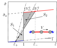
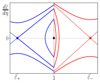
(a) (b)

Figure 1: (a) Stress-strain relation with passive (blue) and active (red) branches. Kink, connecting $\tilde{\varepsilon}_{\pm}$ at the critical value of velocity $V=V_{*}$ when $S_{2}=S_{1}$, is dissipation free. (b) Phase portrait of the continuum system (3) at $1<V<V_{*}$. Stretching pulse corresponds to the homoclinic trajectory starting and ending at $\tilde{\varepsilon}_{+}$; contraction pulse, which exists at $V_{*}<V<V_{**}$, is a homoclinic trajectory starting and ending at $\tilde{\varepsilon}_{-}$ (not shown).

We assume that the constitutive relation for the stress $\sigma$ has two branches: passive and active, see Fig.1(a). For simplicity, the soft elastic response along the passive branch is considered linear $\sigma=E\varepsilon,$ with elastic modulus $E$. To describe the active branch (analog of muscle tetanus), we write $\sigma=\sigma_{a}+E\varepsilon,$ where $\sigma_{a}>0$ is a constant active stress; in more detailed models it can be a variable with sigmoidal response taking a value zero in the passive phase Paoletti and Mahadevan (2014). We further assume that switching from passive to active response takes place when the ’unjamming’ threshold strain $\varepsilon_{c}$ is reached Serra-Picamal et al. (2012). We neglect the possibility of hysteresis and assume that unloading below the threshold $\varepsilon_{c}$ brings the system back into the passive state, see Fig.1(a). To nondimensionalize the system (1) we normalize length by the system size $L$, time by $L/c$, where $c=\sqrt{E/\rho}$, and stress by $E$.

It will be convenient to first deal with a continuum approximation of the discrete problem. To this end we introduce the continuous strain field $\varepsilon(x,t)$, where $\varepsilon(nh,t)=\varepsilon_{n}(t)$ and assume that $h=a/L\ll 1$; we will also use the convenient rescaling $\tilde{u}=u/\varepsilon_{c},\,\tilde{\varepsilon}=\varepsilon/\varepsilon_{c}$ and $\tilde{\sigma}=\sigma/\varepsilon_{c}$. If we now Padé-approximate the nonlocal operator in the right hand side of (1) and leave only the lowest order terms, we obtain Rosenau (1986); Truskinovsky and Vainchtein (2006); Gómez et al. (2012)

$$\left(1-\frac{h^{2}}{12}\frac{\partial^{2}}{\partial x^{2}}\right)\frac{\partial^{2}\tilde{\varepsilon}}{\partial t^{2}}=\frac{\partial^{2}\tilde{\sigma}}{\partial x^{2}}.$$ (2)

To generate a solitary wave solution of (2) we impose a traveling wave anzats $\varepsilon(x,t)=\varepsilon(\eta)$ where $\eta=(x-Vt)/h$ and $V$ is the dimensionless velocity of the pulse.

If we center the active pulse performing local extension at $\eta=0$ and denote its width by $2d$ we can write the associated stress distribution in the form $\tilde{\sigma}(\eta)=\tilde{\varepsilon}(\eta)+\tilde{\sigma}_{a}\text{rect}(\eta/(2d)),$ where $\text{rect}(x)=H(x+1/2)-H(x-1/2)$ and $H(x)$ is the Heaviside function. We require that $\tilde{\varepsilon}(\eta)\to 0$ as $\eta\to\pm\infty$ and impose at $\eta=\pm d$ the matching conditions $\llbracket\tilde{\varepsilon}\rrbracket=\llbracket d\tilde{\varepsilon}/d\eta\rrbracket=0$ and set $\tilde{\varepsilon}(\pm d)=1$. Then, integrating (2) twice and applying the boundary/matching conditions, we obtain the equation

$$\left(V^{2}-1-\frac{V^{2}}{12}\frac{d^{2}}{d\eta^{2}}\right)\tilde{\varepsilon}=\tilde{\sigma}_{a}\text{rect}\left(\frac{\eta}{2d}\right),$$ (3)

where the right hand side implicitly depends on $\tilde{\varepsilon}$. Similar solitary wave solution, describing local contraction , can be obtained if we set $\tilde{\sigma}(\eta)=\tilde{\varepsilon}(\eta)+\tilde{\sigma}_{a}(1-\text{rect}(\eta/(2d)))$ and require that $\tilde{\varepsilon}\to\lambda$ when $\eta\to\pm\infty$ where $\lambda=\tilde{\sigma}_{a}/(V^{2}-1)$. The extension pulses exist in the range $1<V<V_{*}$ where $V_{*}\equiv\sqrt{\tilde{\sigma}_{a}/2+1}$, so they are supersonic which does not mean that they are fast given that the underlying elastic medium is almost an acoustic vacuum Nesterenko (2013). The contraction pulses exist in the range $V_{*}<V<V_{**}$ where $V_{**}\equiv\sqrt{\tilde{\sigma}_{a}+1}>V_{*}$.

The phase portrait of the system (3) at $1<V<V_{*}$ is shown in Fig. 1(b). Two non-degenerate saddle points at $\tilde{\varepsilon}_{\pm}$ lie on the same Rayleigh line $V^{2}=(\tilde{\sigma}(\tilde{\varepsilon})-\tilde{\sigma}(\tilde{\varepsilon}_{+}))/(\tilde{\varepsilon}-\tilde{\varepsilon}_{+})$, see Fig. 1(a). Solitary waves describing the extension pulses, correspond to homoclinic trajectories starting and ending at $\tilde{\varepsilon}_{+}$. Periodic trains of such pulses correspond to closed trajectories encircling the degenerate center at $\tilde{\varepsilon}=1$. As $V\to V_{*}$ homoclinic trajectories become heteroclinic and the solitary waves turn into kinks; at $V=V_{*}$ we have $S_{1}=S_{2}$ in Fig. 1(a) and therefore the associated macroscopic discontinuity is dissipation free Truskinovskii (1982). The structure of these solutions is similar to the one in flocking models Caussin et al. (2014); Solon et al. (2015) modulo the fact that here we omit the explicit description of inflow and outflow of energy. Note that the contraction pulses, which exist in the complimentary range of parameters $V_{*}<V<V_{**}$, correspond to homoclinic trajectories starting and ending at $\tilde{\varepsilon}_{-}$.

In view of the piecewise linear nature of our model, the homoclinic solution of (3) can be written explicitly

$$\tilde{\varepsilon}(\eta)=\begin{cases}\vspace{0.2cm}e^{-(\eta-d)/z},\quad\eta>d,\\ \vspace{0.2cm}\lambda+(1-\lambda)\dfrac{\cosh(\eta/z)}{\cosh(d/z)},\quad-d<\eta<d,\\ e^{(\eta+d)/z},\quad\eta<-d,\end{cases}$$ (4)

where $z=V/\sqrt{12(V^{2}-1)}$ and $\tanh(d/z)=-(1-\lambda)^{-1}.$ Defining the amplitude of the pulse as $A=\max\tilde{\varepsilon}(\eta)-\min\tilde{\varepsilon}(\eta)$, we find for extension pulses that $A=\lambda+(1-\lambda)/\cosh(d/z)$. The corresponding explicit solution for contraction pulses is presented in (SOM, ).

(a)

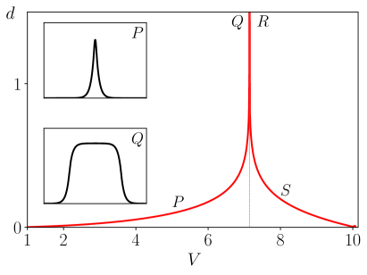
(b)

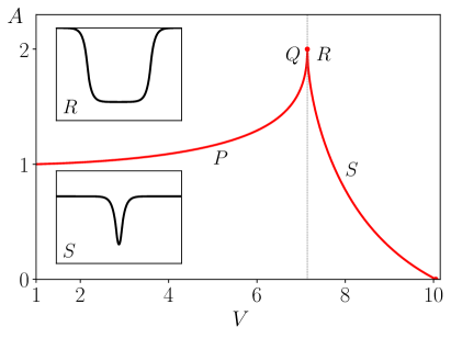
Figure 2: Parametric dependence of the structure of active pulses at $\tilde{\sigma}_{a}=100$: (a) the half-width $d=d(V)$; (b) the amplitude $A=A(V)$; insets show the strain profiles at: $V=5$ (point $P$), $V=V_{*}\pm\delta$, where $\delta=10^{-7}$ (points $Q$ and $R$) and $V=8$ (point $S$). Vertical asymptotes mark the location of the critical point $V=V_{*}$.

The functions $d(V)$ and $A(V)$ for both types of pulses are shown in Fig. 2(a,b). The two families are separated by the critical value of parameter $V=V_{*}$ where the solitary waves take the form of infinitely separated kinks. At this point the parameter $d$, playing the role of the correlation length, diverges even though the pulse amplitude remains finite (taking the value $A=2$). In the limits $V\to 1$ and $V\to V_{**}$ we obtain sonic waves in passive and active states, respectively; note that the passive limit is singular, see (SOM, ) for more details. The typical functions $\tilde{\varepsilon}(\eta)$ for different values of $V$ are shown in the insets in Fig. 2. We emphasize that only the near-critical pulses have a physiologically realistic rectangular form.

Using the relation $\tilde{\varepsilon}=-Vd\tilde{u}/d\eta$, we can obtain the amplitude of the displacement increment culminating the passing of a pulse, for instance, in the case of a stretching pulse $\Delta\tilde{u}=2d\lambda$. As a rough description of a peristaltic wave train, represented by a succession of $N$ such pulses, we can write $\Delta\tilde{u}=2dN\lambda$.

To construct the actual periodic solution we can use the representation $\tilde{\sigma}(\eta)=\tilde{\varepsilon}(\eta)+\tilde{\sigma}_{a}\sum_{j}\text{rect}(\eta-jD/(2d_{p})),$ where it has been assumed that each pulse has a half width $d_{p}$ and the whole active lattice has the period $2D$. The matching conditions are now $\llbracket\tilde{\varepsilon}\rrbracket=\llbracket d\tilde{\varepsilon}/d\eta\rrbracket=0$ and $\tilde{\tilde{\varepsilon}}(jD\pm d_{p})=1$. While the whole solution can be again written explicitly, see SOM , here we only present the transcendental equation for the correlation length $d_{p}$ which is now regularized by the fixed system size $D$: $(1-\lambda)\tanh(d_{p}/z)=\tanh((d_{p}-D)/z).$

The obtained family of solutions is parameterized by $V$ and incorporates both stretching (active) and contraction (passive) pulses. To distinguish between the two it is convenient to re-define the half-width as $d=\min{(d_{p},D-d_{p})}$ and the amplitude as $A=|\tilde{\varepsilon}(0)-\tilde{\varepsilon}(D)|$. The resulting functions $d(V)$ and $A(V)$ are shown in Fig. 3.

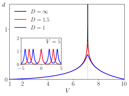
(a) (b)

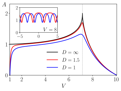
Figure 3: Trains of active pulses at $\tilde{\sigma}_{a}=100$: (a) half-width of a single pulse $d(V)$; (b) its amplitude $A(V)$. Vertical asymptotes correspond to $V=V_{*}$; insets illustrate the typical profiles $\tilde{\varepsilon}(\eta)$.

The obtained periodic solutions can be used to model peristaltic locomotion. Suppose that the organism generates a periodic train of stretching pulses that propagate rearward with a velocity $V$ so that when a pulse reaches the tail, another one is initiated at its head with a fixed delay controlled by the parameter $D$. Observations show that when such pulse moves towards the tail, the latter fattens and gets anchored due to local increase of friction. With such an anchor present, the locomotion naturally occurs into the direction opposite to the direction of the pulse. We mimic such motility pattern in Fig. 4 (left), where the pulse is taken from the range $V<V_{*}$.

Suppose that the motion of the animal is of stick-slip-type with each advance corresponding to passing of a single pulse producing the forward displacement of the head $\Delta\tilde{u}=2d_{p}\lambda$. Since the next pulse arrives after the time $2D/V$, the mean translational velocity of the system is $\overline{v}=\Delta\tilde{u}V/(2D)$. Note that the simultaneous propagation of multiple peristaltic pulses along the animal body is also a possibility which we do not consider here.

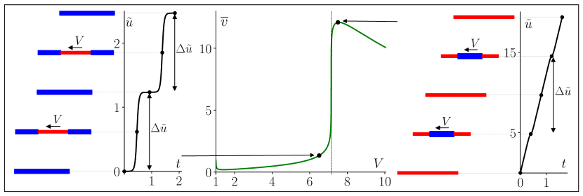
Figure 4: Schematic presentation of peristalsis by trains of active pulses at $\sigma_{a}=100$ and $D=3$. Motility by stretching pulses is shown on the left, by contraction pulses - on the right. The central plot shows dependence of the average velocity $\overline{v}$ on $V$; vertical asymptote corresponds to the critical point at $V=V_{*}$.

The branch of contraction pulses corresponding to $V>V_{*}$ also generates a motility pattern shown in Fig. 4 (right), In this case the ’fattening’ and the resulting anchoring takes place around the pulse. Such regimes, driven by passive pulses in otherwise active medium, are not realistic due to the necessity to maintain active state throughout the whole body of the organism.

The behavior of the function $\overline{v}(V)$ for both kinds of motility ($V\lessgtr V_{*}$ ) is shown in Fig. 4 (center). We emphasize that around the critical point $V=V_{*}$, the macroscopic velocity $\overline{v}$ behaves singularly: it varies over a broad range around a single value of the control parameter. The corresponding individual pulses take the form of elongated rectangles which is one of the most characteristic features of peristaltic waves. Since the width of these rectangular pulses, and therefore the resulting motility velocity, can vary significantly, being positioned near such critical point, can help an organism to adapt its responses. The implied anomalous sensitivity to controls can facilitate optimal behavior in complex physiological conditions and would then be highly functional.

Given that the biological systems exhibiting peristalsis are often segmented, the question arises whether our oversimplified (quasi) continuum model (2) adequately represents the dynamics of its discrete prototype (1). To answer this question we now briefly consider the traveling wave solutions of the original discrete system.

We maintain the same normalization and use again the ansatz $\tilde{\varepsilon}_{n}(t)=\tilde{\varepsilon}(\eta)$, where $\eta=(nh-Vt)/h$. The discrete strain field $\tilde{\varepsilon}(\eta)$ satisfies the equation

$$V^{2}\frac{d^{2}\tilde{\varepsilon}}{d\eta^{2}}=\tilde{\sigma}(\eta+1)+\tilde{\sigma}(\eta-1)-2\tilde{\sigma}(\eta),$$ (5)

with $\tilde{\sigma}(\eta)=\tilde{\varepsilon}(\eta)+\tilde{\sigma}_{a}H(-\eta)$. Solitary wave can be built directly from kinks which we therefore consider first.

Suppose that a switching point where $\tilde{\varepsilon}(0)=1$ is placed at $\eta=0$. Application of the Fourier transform to (5) allows one to obtain an explicit solution:

$$\tilde{\varepsilon}_{k}(\eta)=\tilde{\varepsilon}_{+}-\frac{\tilde{\sigma}_{a}}{2\pi}\int_{-\infty}^{\infty}\frac{\omega^{2}(k)}{(0+ik)L(k)}e^{-ik\eta}\,dk,$$ (6)

where $L(k)=\omega^{2}(k)-(kV)^{2}$, $\omega^{2}(k)=4\sin^{2}\left(k/2\right)$ and $\tilde{\varepsilon}_{+}=\tilde{\varepsilon}(\infty)$. Computing the integral in (6) we obtain the representation of this solution in the form of infinite series

$$\tilde{\varepsilon}_{k}(\eta)=\begin{cases}\vspace{0.2cm}\tilde{\varepsilon}_{+}+\tilde{\sigma}_{a}\sum\limits_{k\in Z^{-}}\dfrac{\omega^{2}(k)}{kL^{\prime}(k)}e^{-ik\eta},\,\eta>0,\\ \tilde{\varepsilon}_{-}-\tilde{\sigma}_{a}\sum\limits_{k\in Z^{+}}\dfrac{\omega^{2}(k)}{kL^{\prime}(k)}e^{-ik\eta},\,\eta>0,\end{cases}$$ (7)

where $Z^{\pm}=\left\{k\,:\,L(k)=0,\,\pm\mathrm{Im}\,k>0\right\}$ and $\tilde{\varepsilon}_{-}=\tilde{\varepsilon}_{+}+\lambda$. This solution exists only for the critical value of velocity $V=V_{*}$, see SOM for details, which suggests that admissible kinks in this model must necessarily satisfy the dynamic Maxwell condition.

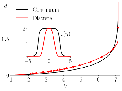
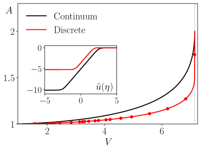
(a) (b)

Figure 5: Comparison of the predictions of discrete (red) and continuum (black) models at $\tilde{\sigma}_{a}=100$ : (a) half-width, (b) amplitude. The red markers show the discrete pulses obtained numerically by solving a one-parametric set of initial value problems. The inserts compare discrete and continuum distributions of strains (a) and displacements (b) at the near critical speed $V=V_{*}-10^{-7}$.

To construct solutions representing stretching pulses we must solve (5) with the stress given by the same rect function as in the continuum case and use the same matching condition $\tilde{\varepsilon}(\pm d)=1$. The linearity of the system at fixed $d$ hints that the solitary wave solution can be obtained as a linear combination of two kinks $\tilde{\varepsilon}(\eta)=\tilde{\varepsilon}_{k}(\eta-d)-\tilde{\varepsilon}_{k}(\eta+d).$ The nonlinear relation $d=d(V)$ can be then found from the matching condition $\tilde{\varepsilon}_{k}(0)-\tilde{\varepsilon}_{k}(2d)=1$. By inverting the equation $(e^{-ik}-1)\hat{u}(k)=\hat{\varepsilon}(k)$ in the Fourier space we can also find the displacement field $u(\eta)$, see SOM , and compute the total displacement which is again $\Delta\tilde{u}=2d\lambda.$ The typical dependencies $d(V),$ and $A(V)$ for stretching pulses are illustrated in Fig. 5, where they are compared with the corresponding results of the continuum theory with $h=1$; the comparison confirms the overall adequacy of the continuum approximation despite the choice of a finite value for our ’small’ parameter.

(a)

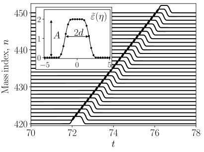
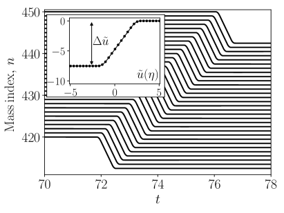
(b)

Figure 6: Results of numerical experiments with discrete chain at $\tilde{\sigma}_{a}=100$ and $v_{0}=200$ (see the text): (a) strains, (b) displacements. The generated stretching pulse correspond to $V\approx V_{*}$, $d\approx 1.88$ and $A\approx 1.998$. Insets show the comparison of the numerical solution in the co-moving frame (markers) with the corresponding analytical solution (solid line).

We tested the numerical stability of the obtained discrete pulses by solving a range of initial value problems. An example of a stable propagation of a rectangular stretching pulse is shown in Fig. 6(a) for the chain with $1000$ springs. We used initial conditions $\tilde{u}_{n}(0)=0,\,\dot{\tilde{u}}_{1}(0)=v_{0}$ and $\dot{\tilde{u}}_{n}(0)=0,\,n>1$ and assumed free ends. The time evolution of the displacement field, shown in Fig. 6(b), illustrates the creation of the main driver of peristaltic motility, the finite displacement behind the propagating pulse.

To conclude, we developed a model of a dynamic passive-to-active transformation taking place in the front of a steadily moving pulse with the corresponding reverse transformation taking place in its rear. The resulting solitary wave solutions for the active medium were extended as periodic trains and used to model the peristaltic mode of self propulsion. We found that at the critical value of parameter the model generates singular regimes with diverging effective correlation length and argued that such criticality may be functional. Our results can be used for biomimetic reproduction of worm-like motion in applications ranging from endoscopic diagnostics Stefanini et al. (2006) to pipeline inspection Yamashita et al. (2011). While in the existing robotic systems activity is usually imitated by globally synchronized distributed actuators Agostinelli et al. (2018); Miller and Dunkel (2020); Jiang and Xu (2017) our focus on local mechanical feedback in muscle-type soft deformable materials opens new avenues in the modeling of peristalsis, see also Pehlevan et al. (2016); Umedachi et al. (2016); DeSimone (2020). The proposed prototypical model can serve only as a proof of concept and future work allowing one to make quantitative predictions, should incorporate energy supply and dissipation and account for realistic 3D geometry.

The authors thank G. Mishuris, P. Recho, A. Vainchtein for helpful discussions and acknowledge the support of the French Agence Nationale de la Recherche under the grant ANR-17-CE08-0047-02.

References

- Sinnott et al. (2017) M. D. Sinnott, P. W. Cleary, and S. M. Harrison, Applied Mathematical Modelling 44, 143 (2017).
- Brandstaeter et al. (2019) S. Brandstaeter, S. L. Fuchs, R. C. Aydin, and C. J. Cyron, GAMM-Mitteilungen 42, e201900001 (2019).
- Gray and Lissmann (1938) J. Gray and H. Lissmann, Journal of Experimental Biology 15, 506 (1938).
- Chapman (1958) G. Chapman, Biological reviews 33, 338 (1958).
- Jones (1978) H. Jones, Journal of Zoology 186, 407 (1978).
- Alexander (1982) R. M. Alexander, Locomotion of animals, Vol. 163 (Springer, 1982).
- Quillin (1999) K. J. Quillin, Journal of Experimental Biology 202, 661 (1999).
- Tyrakowski et al. (2012) T. Tyrakowski, P. Kaczorowski, W. Pawłowicz, M. Ziółkowski, P. Smuszkiewicz, I. Trojanowska, A. Marszaek, M. Żebrowska, M. Lutowska, E. Kopczyńska, et al., Folia biologica 60, 99 (2012).
- Agostinelli et al. (2018) D. Agostinelli, F. Alouges, and A. DeSimone, Frontiers in Robotics and AI 5, 99 (2018).
- Boyle et al. (2012a) J. H. Boyle, S. Berri, and N. Cohen, Frontiers in computational neuroscience 6, 10 (2012a).
- Daltorio et al. (2013) K. A. Daltorio, A. S. Boxerbaum, A. D. Horchler, K. M. Shaw, H. J. Chiel, and R. D. Quinn, Bioinspiration & biomimetics 8, 035003 (2013).
- Boyle et al. (2012b) J. H. Boyle, S. Johnson, and A. A. Dehghani-Sanij, IEEE/ASME Transactions on Mechatronics 18, 439 (2012b).
- Kastberger et al. (2014) G. Kastberger, T. Hoetzl, M. Maurer, I. Kranner, S. Weiss, and F. Weihmann, PloS one 9, e86315 (2014).
- Cartwright (2006) J. H. Cartwright, Europhysics News 37, 22 (2006).
- Solon et al. (2015) A. P. Solon, J.-B. Caussin, D. Bartolo, H. Chaté, and J. Tailleur, Physical Review E 92, 062111 (2015).
- Ngamsaad and Suantai (2018) W. Ngamsaad and S. Suantai, Physical Review E 98, 062618 (2018).
- Dudchenko and Guria (2012) O. Dudchenko and G. T. Guria, Physical Review E 85, 020902 (2012).
- Ijspeert (2008) A. J. Ijspeert, Neural networks 21, 642 (2008).
- Paoletti and Mahadevan (2014) P. Paoletti and L. Mahadevan, Proceedings of the Royal Society B: Biological Sciences 281, 20141092 (2014).
- Miller and Dunkel (2020) P. W. Miller and J. Dunkel, Soft Matter 16, 3991 (2020).
- Prost et al. (2015) J. Prost, F. Jülicher, and J.-F. Joanny, Nature physics 11, 111 (2015).
- Jülicher et al. (2018) F. Jülicher, S. W. Grill, and G. Salbreux, Reports on Progress in Physics 81, 076601 (2018).
- Hawkins and Liverpool (2014) R. J. Hawkins and T. B. Liverpool, Physical review letters 113, 028102 (2014).
- Maitra and Ramaswamy (2019) A. Maitra and S. Ramaswamy, Physical Review Letters 123, 238001 (2019).
- Moshe et al. (2018) M. Moshe, M. J. Bowick, and M. C. Marchetti, Physical review letters 120, 268105 (2018).
- Scheibner et al. (2019) C. Scheibner, A. Souslov, D. Banerjee, P. Surowka, W. Irvine, and V. Vitelli, APS 2019, X53 (2019).
- Raney et al. (2016) J. R. Raney, N. Nadkarni, C. Daraio, D. M. Kochmann, J. A. Lewis, and K. Bertoldi, Proceedings of the National Academy of Sciences 113, 9722 (2016).
- Nadkarni et al. (2014) N. Nadkarni, C. Daraio, and D. M. Kochmann, Physical Review E 90, 023204 (2014).
- Deng et al. (2020) B. Deng, L. Chen, D. Wei, V. Tournat, and K. Bertoldi, Science Advances 6, eaaz1166 (2020).
- Tanaka et al. (2012) Y. Tanaka, K. Ito, T. Nakagaki, and R. Kobayashi, Journal of the Royal Society Interface 9, 222 (2012).
- Kandhari et al. (2019) A. Kandhari, Y. Wang, H. J. Chiel, and K. A. Daltorio, Soft robotics 6, 560 (2019).
- Keller and Falkovitz (1983) J. B. Keller and M. S. Falkovitz, Journal of theoretical biology 104, 417 (1983).
- Wadepuhl and Beyn (1989) M. Wadepuhl and W.-J. Beyn, Journal of theoretical biology 136, 379 (1989).
- Fang et al. (2015) H. Fang, S. Li, K. Wang, and J. Xu, Bioinspiration & biomimetics 10, 066006 (2015).
- Jiang and Xu (2017) Z. Jiang and J. Xu, Micromachines 8, 364 (2017).
- Badoual et al. (2002) M. Badoual, F. Jülicher, and J. Prost, Proceedings of the National Academy of Sciences 99, 6696 (2002).
- Serra-Picamal et al. (2012) X. Serra-Picamal, V. Conte, R. Vincent, E. Anon, D. T. Tambe, E. Bazellieres, J. P. Butler, J. J. Fredberg, and X. Trepat, Nature Physics 8, 628 (2012).
- Rosenau (1986) P. Rosenau, Physics Letters A 118, 222 (1986).
- Truskinovsky and Vainchtein (2006) L. Truskinovsky and A. Vainchtein, Continuum Mechanics and Thermodynamics 18, 1 (2006).
- Gómez et al. (2012) L. R. Gómez, A. M. Turner, and V. Vitelli, Physical Review E 86, 041302 (2012).
- Nesterenko (2013) V. Nesterenko, Dynamics of heterogeneous materials (Springer Science & Business Media, 2013).
- Truskinovskii (1982) L. M. Truskinovskii, in Doklady Akademii Nauk, Vol. 265 (Russian Academy of Sciences, 1982) pp. 306–310.
- Caussin et al. (2014) J.-B. Caussin, A. Solon, A. Peshkov, H. Chaté, T. Dauxois, J. Tailleur, V. Vitelli, and D. Bartolo, Physical review letters 112, 148102 (2014).
- (44) See Supplemental Material at [URL will be inserted by publisher] for [give brief description of material].
- Stefanini et al. (2006) C. Stefanini, A. Menciassi, and P. Dario, The International Journal of Robotics Research 25, 551 (2006).
- Yamashita et al. (2011) A. Yamashita, K. Matsui, R. Kawanishi, T. Kaneko, T. Murakami, H. Omori, T. Nakamura, and H. Asama, in 2011 IEEE International Conference on Robotics and Biomimetics (IEEE, 2011) pp. 1017–1023.
- Pehlevan et al. (2016) C. Pehlevan, P. Paoletti, and L. Mahadevan, Elife 5, e11031 (2016).
- Umedachi et al. (2016) T. Umedachi, T. Kano, A. Ishiguro, and B. A. Trimmer, Royal Society open science 3, 160766 (2016).
- DeSimone (2020) A. DeSimone, in The Mathematics of Mechanobiology (Springer, 2020) pp. 1–41.