Thermodynamic properties of the finite–temperature electron gas
by the fermionic path integral Monte Carlo method

Abstract

The new ab initio quantum path integral Monte Carlo approach has been developed and applied for the entropy difference calculations for the strongly coupled degenerated uniform electron gas (UEG), a well–known model of simple metals. Calculations have been carried out at finite temperature in canonical ensemble over the wide density and temperature ranges. Obtained data may be crucial for density functional theory. Improvements of the developed approach include the Coulomb and exchange interaction of fermions in the basic Monte Carlo cell and its periodic images and the proper change of variables in the path integral measure. The developed approach shows good agreement with available results for fermions even at temperature four times less than the Fermi energy and practically doesn’t suffer from the “fermionic sign problem”, which takes place in standard path integral Monte Carlo simulations of degenerate fermionic systems. Presented results include pair distribution functions, isochors and isotherms of pressure, internal energy and entropy change in strongly coupled and degenerate UEG in a wide range of density and temperature.

I Introduction

Entropy is a fundamental quantity in physics and is recognized as one of the most important and enigmatic concepts in nature Martin and England (2011). In the studies of phase stability, phase transitions and reaction directions the free energies and entropies corresponding to the desired phases or reaction states are the most properties of interest. In this paper we applied the concepts of entropy to consideration of the one-component plasma (OCP), being a fundamental many-body model consisted of a single specie of charged particles, immersed in a rigid neutralizing background. For electrons, OCP is often called “uniform electron gas” (UEG) or “jellium” and can be used as a model of simple metals. Even though UEG itself does not represent a real physical system, its accurate description is crucial for density functional theory (DFT) Kohn and Sham (1965); Hohenberg and Kohn (1964); Filinov et al. (2020).

Accurate data for the electron gas of the highly excited systems at finite temperatures, such as warm dense matter have been obtained by the path integral Monte Carlo (PIMC) techniques Feynman et al. (2010); Binder and Ciccotti (1996); Ceperley (1995); Zamalin et al. (1977); Filinov et al. (2006); Egger et al. (1999); Filinov et al. (2001) and for dense plasma in Militzer and Pollock (2000); Militzer (2006); Filinov et al. (2000) . These results have been used for DFT calculations as a basis for the local (spin-)density approximation (L(S)DA) and more sophisticated gradient approximations Karasiev et al. (2016); Ramakrishna et al. (2020); Karasiev et al. (2019a); Karasiev et al. (2014); Karasiev et al. (2019b); Dornheim et al. (2018); Perdew et al. (1996a, b).

The cornerstone difficulty in the path integal Monte Carlo (PIMC) simulations of quantum fermions is the “fermionic sign problem”. Reliable Monte Carlo simulations at finite temperature in wide fermion density range have been carried out by a permutation blocking (PB) PIMC approach Dornheim et al. (2015a, 2016a) and the configurational PIMC approach (CPIMC) Schoof et al. (2011a, 2015a, b, 2015b); Groth et al. (2016); Dornheim et al. (2015b); Malone et al. (2015, 2016); Blunt et al. (2014). The Dornheim, Groth and co-workers Dornheim et al. (2015b, 2016b) have developed an formalism, which allows to approach the thermodynamic limit and construct a highly accurate parametrization of the UEG exchange-correlation free energy. On the other habd the approach proposed in Larkin et al. (2017a, b) is based on the Wigner formulation of quantum mechanics. This approach has been realized the Pauli blocking of fermions without antisymmetrization of matrix elements as it used the derived effective pair pseudopotential in phase space preventing occupation of a quantum phase space cell by the two identical fermions.

However data for entropy of the strongly coupled UEG are still unknown. Widely used approaches to calculate the entropy in canonical ensemble at finite temperature for arbitrary system of particles are based on the thermodynamic integration Frenkel and Smit (2001) and nonequilibrium work relations such as the Jarzynski equality Jarzynski (1997) for the determination the changes in the free-energy and allowing to obtain the entropy difference. The microcanonical equivalent of the Jarzynski equality Adib (2005) was used to calculate isoenergetic entropy differences using a switching parameter. The Wang-Landau techniques Wang and Landau (2001a, b); Shell et al. (2002); Davis (2011) for the determination of entropy consist of performing a random walk in energy space to achiev a flat histogram of energies.

The motivation of the present work is to perform ab initio direct fermionic PIMC (FPIMC) simulations to calculate entropy at finite temperature in canonical ensemble. We modify the direct PIMC approach, that previously has been successfully applied to dense hydrogen, hydrogen-helium mixtures, electron-hole plasmas in semiconductors and nonideal quark–gluon plasma Ebeling et al. (2017). To reduce the finite size effects of FPIMC and the influence of artificial periodic boundary conditions in the interparticle interaction we use the scheme proposed by Yakub et al. Yakub and Ronchi (2003). Here we have developed the same ideas to describe exchange interaction between fermions. The numerical results presented in this article demonstrate the significant reducing of the “fermionic sign problem”. In section 2 we describe the basic concepts of the UEG model, its path integral description and mathematical formalism for entropy change calculations. In section 3 we present obtaines results for pair distribution functions, pressure and internal energy on the isochors and isotherms and the entropy changes in the strongly coupled and degenerate UEG in a wide range of density and temperature. Developed approach reveals good reliability for temperatures in several times less than the Fermi energy. In section 4 we present some concluding remarks and possible perspectives.

II Fermionic path integral Monte Carlo simulations

II.1 Jellium model

UEG, or jellium, is a quantum mechanical model of interacting electrons on a rigid neutralizing background. This model allows one to treat the quantum effects of electrons and their repulsive interaction rigorously. In this article we are going to simulate thermodynamic properties of strongly coupled UEG. Due to the strong electron interaction and absence of small physical parameters we can not use analytical methods based on different perturbation theories and have to deal with the density matrix of the system. Our efforts in this direction have resulted in the development of a new “ab initio” quantum fermionic path integral Monte Carlo approach (FPIMC) Filinov et al. (2020). The UEG Hamiltonian contains the electron kinetic ${\hat{K}}$ and Coulomb energy ${\hat{U}}^{c}_{ee}$ contributions, the interaction of electrons with the neutralizing background ($\hat{U}^{c}_{ep}$) and the self-interaction energy of the background ($\hat{U}^{c}_{pp}$). The rigid neutralizing background is simulated as an ideal gas of uncorrelated classical positive charges uniformly distributed in space. The path integral representation of density matrix is used to obtain the UEG partition function and thermodynamic properties. A number of modifications to the standard PIMC scheme discussed below allowed us to significantly reduce the influence of the notorious “fermionic sign problem”.

Let us consider a neutral two-component Coulomb system of quantum electrons and classical positive charges in equilibrium with the general Hamiltonian, ${\hat{H}}={\hat{K}}+{\hat{U}}^{c}$, containing kinetic energy ${\hat{K}}$ and Coulomb interaction energy contributions, ${\hat{U}}^{c}={\hat{U}}_{pp}^{c}+{\hat{U}}^{c}_{ee}+{U}^{c}_{ep}$.

The thermodynamic properties in the canonical ensemble with a given temperature $T$ and fixed volume $V$ are fully described by the density operator ${\hat{\rho}}=e^{-\beta{\hat{H}}}$, with the partition function

$$Z(N_{e},N_{p},V;\beta)=\frac{1}{N_{e}!N_{p}!}\sum_{\sigma}\int\limits_{V}\rm dx\,\rho(x,\sigma;\beta),$$ (1)

where $\beta=1/k_{B}T$, and $\rho(q,\sigma;\beta)$ denotes the diagonal elements of the density matrix in the coordinate representation at a given value $\sigma$ of the total spin. In Eq. (1), $x=\{x_{e},x_{p}\}$ and $\sigma=\{\sigma_{e}\}$ are the spatial coordinates (in units of thermal wave lengths) of electrons and positive charges and spin degrees of freedom of the electrons, i.e. $x_{a}=\{x_{1,a}\ldots x_{l,a}\ldots x_{N_{a},a}\}$ and $\sigma_{e}=\{\sigma_{1,e}\ldots\sigma_{l,e}\ldots\sigma_{N_{e},e}\}$. The exact density matrix of interacting quantum systems is not known (particularly at low temperatures and high densities), but can be constructed using a path integral representation Feynman et al. (2010) based on the operator identity,

$$e^{-\beta{\hat{H}}}=e^{-\epsilon{\hat{H}}}\cdot e^{-\epsilon{\hat{H}}}\dots e^{-\epsilon{\hat{H}}},\quad\epsilon=\beta/(M+1)$$ (2)

that involves $M+1$ identical high-temperature factors with a temperature $(M+1)T$, which allows us to rewrite the integral in Eq. (1) as

$$\sum_{\sigma}\int\limits\rm dx^{(0)}\,\rho(x^{(0)},\sigma;\beta)=\int\limits\rm dx^{(0)}\dots\rm dx^{(M)}\,\rho^{(1)}\,\dots\rho^{(m)}\,\dots\rho^{(M-1)}\times$$

$$\sum_{\sigma}\sum_{P_{e}}(-1)^{\kappa_{P_{e}}}\,{\cal S}(\sigma,{\hat{P}_{e}}\sigma_{a}^{\prime})\,\times{\hat{P}_{e}}\rho^{(M)}\big{|}_{x^{(M+1)}=x^{(0)},\sigma^{\prime}=\sigma},$$ (3)

where index $m=0,\dots,M$ labels the off–diagonal high–temperature density matrices $\rho^{(m)}\equiv\rho\left(x^{(m)},x^{(m+1)};\epsilon\right)=\langle x^{(m)}|e^{-\epsilon{\hat{H}}}|x^{(m+1)}\rangle$. The spin gives rise to the spin part of the density matrix (${\cal S}$) with exchange effects accounted for by the permutation operator $\hat{P}_{e}$ acting on the electron coordinates $q^{(M+1)}$ and spin projections $\sigma^{\prime}$. The sum is over all permutations with parity $\kappa_{P_{e}}$.

Let us consider the off-diagonal elements of the density matrix $\rho(\tilde{x},\sigma;x^{\prime},\sigma^{\prime};\beta)$. With the error of order $1/M^{2}$, arising from neglecting the commutator $\epsilon^{2}/2\left[K,U^{c}\right]$, each high-temperature factor can be presented in the form $\langle x^{(m)}|e^{-\epsilon{\hat{H}}}|x^{(m+1)}\rangle\approx\langle x^{(m)}|e^{-\epsilon{\hat{U}_{m}}}|x^{(m+1)}\rangle\rho^{(m)}_{0}$, where $\rho^{(m)}_{0}=\langle x^{(m)}|e^{-\epsilon{\hat{K}}}|x^{(m+1)}\rangle$. The off-diagonal density matrix element involves an effective pair interaction $U=\sum_{k,t}\Phi_{kt}$, which is approximated by its diagonal elements according to $\Phi^{OD}_{kt}(q_{k,a},q^{\prime}_{k,a},q_{t,b},q^{\prime}_{t,b};\epsilon)\approx\frac{1}{2}[\Phi_{ab}(q_{k,a}-q_{t,b};\epsilon)+\Phi_{ab}(q^{\prime}_{k,a}-q^{\prime}_{t,b};\epsilon)]$, where the effective potential (the Kelbg potential) is given by the expression Ebeling et al. (2017):

$$\Phi_{ab}(x_{ab};\epsilon)=\frac{e_{a}e_{b}}{\tilde{\lambda}_{ab}x_{ab}}\left[1-e^{-x_{ab}^{2}}+\sqrt{\pi}x_{ab}\left\{1-{\rm erf}(x_{ab})\right\}\right].$$ (4)

Here $\tilde{\lambda}_{ab}x_{ab}=|q_{k,a}-q_{t,b}|\tilde{\lambda}_{e}$, $\tilde{\lambda}^{2}_{ab}=2\pi\hbar^{2}\epsilon/m_{ab}$, $1/m_{ab}=1/m_{a}+1/m_{b}$, $\tilde{\lambda}^{2}_{e}=2\pi\hbar^{2}\epsilon/m_{e}$ and ${\rm erf}(x)$ is the standard error function.

Note that the Kelbg potential is finite at zero distance, due to it’s quantum nature. This is a crucial advantage of the Kelbg potential over the Coulomb potential in simulations of systems with attractive Coulomb interaction. At the interparticle distance more than the thermal wavelength the Kelbg potential coincides with the Coulomb one. Then the off-diagonal elements of the density density matrix are:

$$\rho(\tilde{x},\sigma;x^{\prime},\sigma^{\prime};\beta)=\sum_{\sigma}\sum_{P_{e}}(\pm 1)^{\kappa_{P_{e}}}{\cal S}(\sigma,{\hat{P}_{e}}\sigma^{\prime})\langle x-\xi/2|\prod_{m=0}^{M-1}e^{-\epsilon{\hat{U}_{m}}}e^{-\epsilon{\hat{K}_{m}}}|{\hat{P}_{e}}(x+\xi/2)\rangle,$$ (5)

where $\tilde{x}=x-\xi/2$ and $x^{\prime}=x+\xi/2$ and $x\equiv x^{(0)}$. In the limit $M\rightarrow\infty$ the error of the whole product of high temperature factors is equal to zero $(\propto 1/M)$, and we have an exact path integral representation of the partition function. Here each particle is presented by an “open” trajectory consisting of a set of $M$ coordinates $x^{(m)}$ (“beads”).

It is important that these matrix elements of the density matrix can be rewritten in the form of the path integral over “closed” trajectories starting and ending at zero ($\eta^{(0)}=\eta^{(M)}=\bf 0$) Filinov et al. (2020):

$$\rho(x,\sigma;x^{\prime},\sigma^{\prime};\beta)\big{|}_{x=x^{\prime},\sigma^{\prime}=\sigma}\,\approx\,\int\rm d\eta^{(1)}\dots\rm d\eta^{(M-1)}\exp\Biggl{\{}-\sum\limits_{m=1}^{M-1}\biggl{[}\pi|\eta^{(m)}|^{2}+\epsilon U\biggl{(}x+\sum_{k^{\prime}=0}^{m}\eta^{(k^{\prime})}\biggr{)}\biggr{]}\Biggr{\}}{\rm det}||\psi(x)||,$$ (6)

and we define

$$||\psi(x)|| = \left\|e^{-{\pi}\left|r_{kt}/M\right|^{2}}\right\|_{\frac{N_{e}}{2}}\times\left\|e^{-{\pi}\left|\tilde{r}_{kt}/M\right|^{2}}\right\|_{\frac{N_{e}}{2}}.$$ (7)

Here we introduce the following notation for the dimensionless coordinate $r_{kt}\equiv(x_{k,e}-x_{t,e}),\quad(k,t=1,\dots,N_{e}/2),\tilde{r}_{kt}\equiv(x_{k,e}-x_{t,e}),\quad(k,t=N_{e}/2+1,\dots,N_{e})$ and assume that in the thermodynamic limit the main contribution to the sum over spin variables comes from the term related to the equal number ($N_{e}/2$) of electrons with the same spin projection.

In order to calculate thermodynamic functions in the canonical ensemble, the logarithm of the partition function has to be differentiated by variables $T$ and $V$. For example, for pressure and internal energy:

$$\beta p = \frac{\partial{\rm ln}Z}{\partial V}=\left[\frac{\alpha}{3V}\frac{\partial{\rm ln}Z}{\partial\alpha}\right]_{\alpha=1},$$ (8)

$$\beta E = -\beta\frac{\partial{\rm ln}Z}{\partial\beta},$$ (9)

where $\alpha=L/L_{0}$ is a length scaling parameter. For pressure we have:

$$\frac{\beta pV}{N_{e}+N_{p}}=1-\frac{(3Z)^{-1}}{N_{e}+N_{p}}\times\int dxd\eta^{(1)}\dots\rm d\eta^{(M-1)}\,$$

$$\times\exp\Biggl{\{}-\sum\limits_{m=0}^{M-1}\biggl{[}\pi|\eta^{(m)}|^{2}+\epsilon U\biggl{(}x+\sum_{k^{\prime}=0}^{m}\eta^{(k^{\prime})}\biggr{)}\biggr{]}\Biggr{\}}{{\rm det}||\psi||}$$

$$\times\Bigg{\{}\sum_{k=1}^{N_{p}}\sum_{t=1}^{N_{e}}|x_{kt}|\frac{\partial\epsilon\Phi_{ep}}{\partial|x_{kt}|}+\sum_{k<t}^{N_{p}}|x_{kt}|\frac{\partial\epsilon\Phi_{pp}}{\partial|x_{pt}|}+\sum_{k<t}^{N_{e}}|x_{kt}|\frac{\partial\epsilon\Phi_{ee}}{\partial|x_{kt}|}$$

$$+\sum_{m=0}^{M-1}\Big{(}\sum_{k=1}^{N_{p}}\sum_{t=1}^{N_{e}}B(x^{m}_{kt})\frac{\partial\epsilon\Phi_{ep}}{\partial|x^{m}_{kt}|}+\sum_{k<t}^{N_{e}}A(x^{m}_{kt})\frac{\partial\epsilon\Phi_{ee}}{\partial|x^{m}_{kt}|}+\sum_{k<t}^{N_{p}}A(x^{m}_{kt})\frac{\partial\epsilon\Phi_{pp}}{\partial|x^{m}_{kt}|}\Big{)}$$

$$-\frac{\alpha}{{\rm det}||\psi||}\frac{\partial{\rm\,det}||\psi||}{\partial\alpha}\Bigg{\}}|_{\alpha=1},$$ (10)

where $B(x^{m}_{kt})=\frac{\langle x^{m}_{pt}|x_{kt}\rangle}{|x^{m}_{pt}|}$, $A(x^{m}_{kt})=\frac{\langle x^{m}_{kt}|x_{kt}\rangle}{|x^{m}_{kt}|}$.

II.2 Reducing the finite size effects

Computer simulations of disordered systems, such as plasmas, require an accurate accounting of the long–range Coulomb forces. To reduce the finite–size effects in the PIMC simulations periodic boundary conditions (PBC) are usually imposed on the main Monte Carlo cell and the Ewald summation method is used to calculate the contribution of its periodic images. For high electron degeneracy the thermal wavelength $n\lambda^{3}$ can exceed the main MC cell size $L$. Therefore the trajectories of electrons in the main cell can penetrate into periodic neighboring images of the main cell. This issue requires modified PBC in the treatment of the exchange interaction in PIMC simulations. The modification of PBC in this case is discussed in Ebeling et al. (2017). In addition, it is necessary to take into account the exchange interaction between particles in the main MC cell and their periodic images.

To take into account the exchange and long–range Coulomb interaction between particles of the main MC cell and its periodic images, we can redefine the related MC estimators. The corresponding technique and the energy estimator can be found elsewhere Filinov et al. (2020). For pressure the estimator replace Eq. (10) has the following modified form:

$$\frac{\beta pV}{N_{e}+N_{p}} = 1-\frac{(3Z)^{-1}}{\,N_{e}+N_{p}}\times$$ (11)

$$\times\int dx\mathrm{d\eta^{(1)}\dots d\eta^{(M-1)}}\,\exp\Biggl{\{}-\sum\limits_{m=0}^{M-1}\biggl{[}\pi|\eta^{(m)}|^{2}+\epsilon\tilde{U}\biggl{(}x+\sum_{k^{\prime}=0}^{m}\eta^{(k^{\prime})}\biggr{)}\biggr{]}\Biggr{\}}{\rm det}||\psi(x)||$$

$$\times\Bigg{\{}\sum_{\boldsymbol{n}}\Bigg{(}\sum_{k=1}^{N_{p}}\sum_{t=1}^{N_{e}}|x_{kt}|\frac{\partial\epsilon\Phi_{ep}\Big{(}\boldsymbol{n}L+x\Big{)}}{\partial|x_{kt}|}+\sum_{k<t}^{N_{p}}|x_{kt}|\frac{\partial\epsilon\Phi_{pp}\Big{(}\boldsymbol{n}L+x\Big{)}}{\partial|x_{pt}|}+\sum_{k<t}^{N_{e}}|x_{kt}|\frac{\partial\epsilon\Phi_{ee}\Big{(}\boldsymbol{n}L+x\Big{)}}{\partial|x_{kt}|}\Bigg{)}$$

$$+\sum_{m=0}^{M-1}\sum_{\boldsymbol{n}}\Bigg{(}\sum_{k=1}^{N_{p}}\sum_{t=1}^{N_{e}}B(x^{m}_{kt})\frac{\partial\epsilon\Phi_{ep}\Big{(}(\boldsymbol{n}L+x+\sum_{k^{\prime}=0}^{m}\eta^{(k^{\prime})})^{m}_{kt}\Big{)}}{\partial|x^{m}_{kt}|}+$$

$$+\sum_{k<t}^{N_{e}}A(x^{m}_{kt})\frac{\partial\epsilon\Phi_{ee}(\boldsymbol{n}L+x+\sum_{k^{\prime}=0}^{m}\eta^{(k^{\prime})})^{m}_{kt}}{\partial|x^{m}_{kt}|}$$

$$+\sum_{k<t}^{N_{p}}A(x^{m}_{kt})\frac{\partial\epsilon\Phi_{pp}(\boldsymbol{n}L+x+\sum_{k^{\prime}=0}^{m}\eta^{(k^{\prime})})^{m}_{kt}}{\partial|x^{m}_{kt}|}\Bigg{)}$$

$$-\frac{\alpha}{{\rm det}||\psi(x)||}\frac{\partial\sum_{\boldsymbol{n}}{\rm\,det}||\psi(\boldsymbol{n}L+x)||}{\partial\alpha}|_{\alpha=1}\Bigg{\}},$$

where $\tilde{U}=U_{ee}$ as the positive charges simulating neutralizing rigid background have to be uncorrelated.

We also use a modified Ewald scheme proposed by Yakub Yakub and Ronchi (2003) to eliminate artificial non-isotropic effects caused by PBC. The generalization of this scheme using the angle averages for electrostatic (via the Kelbg potential) and exchange interactions Filinov et al. (2020).

II.3 Basic expressions for the entropy change

During an expansion of a system of particles both temperature and volume may change. Then the total entropy change $dS(T,V)$ is:

$$dS(T,V)=\left(\frac{\partial S}{\partial T}\right)_{V}dT+\left(\frac{\partial S}{\partial V}\right)_{T}dV.$$ (12)

To calculate the entropy change between two states $S(T_{2},V_{2})-S(T_{1},V_{1})$ we can do integration first at constant $V$ and then at constant $T$

$$S(T_{2},V_{2})-S(T_{1},V_{2})=\int_{T_{1}}^{T_{2}}\left.\left(\frac{\partial S}{\partial T}\right)\right|_{V=V_{2}}dT,\quad S(T_{1},V_{2})-S(T_{1},V_{1})=\int_{V_{1}}^{V_{2}}\left.\left(\frac{\partial S}{\partial V}\right)\right|_{T=T_{1}}dV.$$ (13)

Here as an application of the developed approach we are going to calculate the entropy change by integrating over $T$ and $V$:

$$\Delta S_{V_{2}}=S(T_{2},V_{2})-S(T_{1},V_{2})=\int_{T_{1}}^{T_{2}}\left.\left(\frac{\partial S}{\partial T}\right)\right|_{V=V_{2}}dT=\int_{T_{1}}^{T_{2}}\left.\left(\frac{C_{V}}{T}\right)\right|_{V=V_{2}}dT=\int_{T_{1}}^{T_{2}}\left.\left(\frac{1}{T}\frac{\partial E}{\partial T}\right)\right|_{V=V_{2}}dT,$$ (14)

$$\Delta S_{T_{1}}=S(T_{1},V_{2})-S(T_{1},V_{1})=\int_{V_{1}}^{V_{2}}\left.\left(\frac{\partial S}{\partial V}\right)\right|_{T=T_{1}}dV=\int_{V_{1}}^{V_{2}}\left.\left(\frac{\partial P(T,V)}{\partial T}\right)\right|_{V}dV$$ (15)

where we use the Maxwell relation for the derivatives of entropy and pressure based on the equalities of the second derivatives of Helmholtz free energy $F$:

$$\left(\frac{\partial S}{\partial V}\right)_{T}=-\frac{\partial^{2}F(T,V)}{\partial V\partial T}=-\frac{\partial^{2}F(T,V)}{\partial T\partial V}=\left(\frac{\partial P}{\partial T}\right)_{V}.$$ (16)

III Simulation results

III.1 Pair distribution functions

To calculate UEG pressure and energy we use the estimators with the PBC modifications discussed above. We have considered electron density defined by the Brueckner parameter $r_{s}=\langle r\rangle/a_{B}$ in the range $0.7\leq r_{s}\leq 1$ and temperature of the system in the range $1.73\leq T/\text{Ry}\leq 2$, where $\langle r\rangle$ is the mean distance between electrons, $a_{B}$ is the Bohr radius, Ry is hydrogen ionization energy.

Let us start from the physical analysis of the spatial arrangement of electrons and positive particles, simulating the rigid neutralizing background, by studying the radial distribution function (RDF) $g_{ab}(R)$ defined as:

$$g_{ab}(|{\bf R}_{1}-{\bf R}_{2}|) = \left(\frac{V}{N}\right)^{2}\sum_{\sigma}\sum_{i,j,i\neq j}\delta_{a_{i},a}\,\delta_{a_{j},b}\frac{1}{Z}\int\rm dr\;\delta({\bf R}_{1}-{\bf r}_{i})\,\delta({\bf R}_{2}-{\bf r}_{j})\;\,\rho(x,\sigma;\beta),$$ (17)

where $a_{i}$ and $b_{j}$ denote the types of particles. The RDF depends only on the difference of coordinates $R=|{\bf R}_{1}-{\bf R}_{2}|$ because of the translational invariance of the system. In a non-interacting classical system $g_{ab}(R)\equiv 1$, whereas interparticle interactions and quantum statistics result in a redistribution of particles. The product $R^{2}g_{ab}(R)$ is proportional (up to a constant factor) to the probability to find a pair of particles at a distance $R$ from each other.

As an example different RDFs averaged over spin of electrons are shown in Fig. 1a for a temperature $T=2\text{Ry}$ and density related to $r_{s}=0.8$. The positive particles are uncorrelated as they are simulating the positive rigid background in UEG and $g_{pp}$ and $g_{ep}$ RDFs are identically equal to unity as in ideal gas.

The electron-electron RDF $g_{ee}$ demonstrates a drastic difference at short distances due to the Coulomb and Fermi repulsion. Here $g_{ee}$ decreases monotonically when the interparticle distance goes to zero but tends to unity in the opposite case. Oscillations of the RDF at very small distances are related to Monte-Carlo statistical error, as the probability to find particles at short distances quickly decreases.

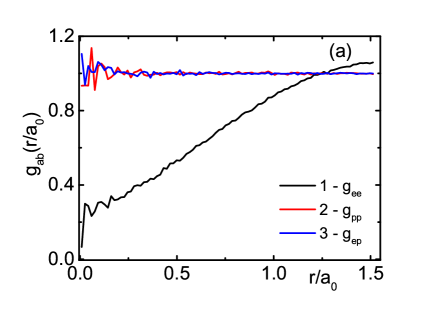
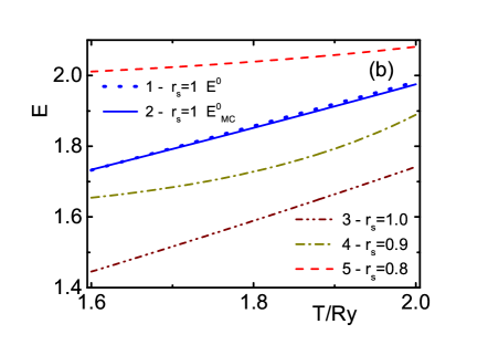
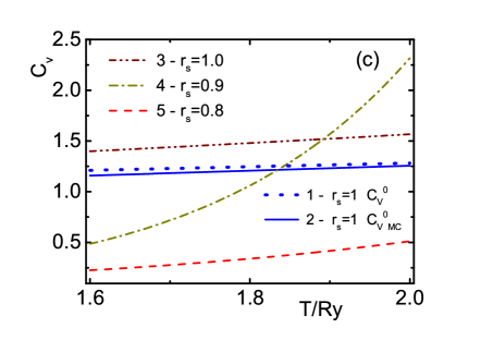
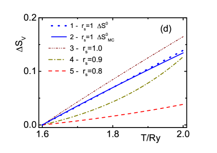
Figure 1: (Color online) (a) Electron—electron, positive charge—positive charge and electron—positive charge RDFs at temperatures $T/\text{Ry}=2$ and $r_{s}=0.8$; (b) isochores of internal energy; (c) heat capacity at constant volume; (d) entropy change of UEG. Line 1: analytical dependences for ideal UEG at $r_{s}=1$. The FPIMC simulation results for ideal UEG at $r_{s}=1$ - line 2; for strongly coupled UEG at: $r_{s}=0.8$—line 3; $r_{s}=0.9$—line 4; $r_{s}=1$—line 5.

III.2 Entropy changes on isochores and isotherms

Plots (b), (c) and (d) in Figure 1 present internal energy, isochoric heat capacity and entropy change on different isochores for UEG in the temperature range $1.6\text{Ry}$–$2\text{Ry}$. Comparison with ideal UEG in Figure 1(b) shows that the interparticle interaction downgrades the internal energy at $r_{s}\sim 1-0.9$ (degeneracy parameter $n\lambda^{3}\sim 3-5$ and coupling parameter $\Gamma\sim 1$), but then raises it with the growth of electron density ($r_{s}\sim 0.8$, degeneracy parameter $n\lambda^{3}\sim 8$ and practically the same coupling parameter $\Gamma\sim 1-2$).

In Figure 1(c) heat capacity equal to the derivative of the internal energy with respect to temperature demonstrates more complicated behavior at temperatures less and more than $T/\text{Ry}\sim 1.8$ that can be the consequence of the interplay of the electron interaction and Fermi repulsion. Stronger electron degeneracy at $r_{s}\lesssim 0.9$ and $T/\text{Ry}\lesssim 1.8$ results in the heat capacity decrease (lines 4 and 5) in comparison with the ideal UEG. Just on the contrary at lower density ($r_{s}\sim 1$) and $T/\text{Ry}\gtrsim 1.8$ heat capacity (lines 3 and 4) is larger than that in the ideal UEG.

Entropy change in Figure 1(d) more or less repeats the behavior of heat capacity as entropy is defined by the antiderivative of the ratio of heat capacity to temperature according to Eq. 14.

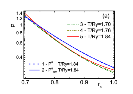
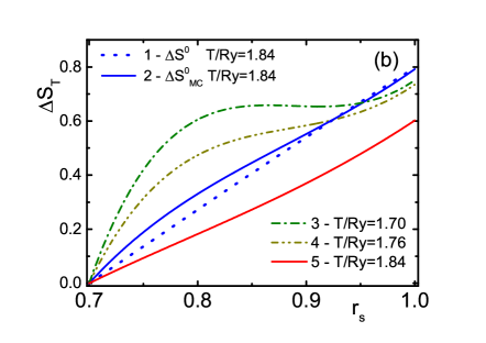
Figure 2: (Color online) Pressure (a) and entropy change (b) of UEG on isotherms. Analytical dependences for ideal UEG at $T/Ry=1.84$ are shown by lines 1. The FPIMC simulation results are: ideal UEG at $T/Ry=1.84$—line 2; strongly coupled UFG at $T/Ry=1.70$—line 3; at $T/Ry=1.76$—line 4; at $T/Ry=1.84$—line 5.

Figure 2 shows pressure and entropy change of UEG on isotherms in the range of $r_{s}$ 0.7–1. Isotherms for pressure and entropy change of the strongly coupled UEG are presented by lines 3–5. Particle interaction in UEG results in decreasing pressure in comparison with the ideal UEG at low density ($r_{s}\geq 0.75$). The opposite situation is at higher density ($r_{s}\leq 0.75$), where the Fermi repulsion is more important. From the analysis of pressure in Figure 2(a) we can expect that the derivate of pressure with respect to temperature is a decreasing function of $r_{s}$ as the typical difference in pressure at fixed $r_{s}$ on the left hand side of Figure 2(a) is larger than the same difference on the right hand side of the same plot, while in between this difference is approaching zero. Consequently, according to Eq. 15 the change in entropy equals to the antiderivative over volume of the function $\frac{\partial P(T,V)}{\partial T}|_{T}$ can monotonically or non-monotonically increase versus $r_{s}$, as shown in Figure 2(b).

III.3 Error estimations

According to Eqs. (14) and (15) entropy change is defined by the integral over the derivatives of pressure and internal energy with respect to temperature. In the used FPIMC approach these derivatives can not be directly calculated and have been obtained by the numerical differentiation of the smoothed FPIMC results for these functions on the corresponding isotherms and isochores. Sure the accuracy of numerically obtained derivatives is lower than the accuracy of the same values calculated directly (by any other MC method). Moreover errors in calculations of entropy change can be accumulated at integration over the obtained approximations of derivatives according to Eqs. (14) and (15).

As an example, the estimation of the accuracy of the presented FPIMC results for entropy change can be obtained from the comparison of lines 1 and 2 presenting entropy change for ideal UEG in Figure 1(d). Here line 1 presents the analytical dependence, while line 2 shows the FPIMC results for the ideal UEG. The accuracy of the used numerical differentiation is high enough for reliable analysis of the main features of the physical behavior of presented data. We plan to eliminate the small discrepancy in entropy change from the analytical model in the future.

The main source of errors in PIMC simulations is the correct accounting of exchange interaction. As we mentioned above the developed FPIMC demonstrates a good accuracy for the degenerate ideal UEG and moreover as it follows from the paper Filinov et al. (2020) this is also true for the strongly coupled degenerate UEG.

IV Discussion

This contribution presents a new PIMC approach and first results for pressure and entropy difference of the degenerate and strongly coupled electron gas. Knowledge of these quantities is of great interest in the study of thermodynamics and can also be used for physical explanations of the experimental observations. Advantage of the developed approach is that it works in a broad density–temperature range because it takes into account Coulomb and exchange interaction not only in the main MC cell but also in surrounding periodic images. Several improvements have been made. The first one is a proper change of variables modifying the path integral measure and exchange determinant. Then we use the angle–averaged long–range Coulomb interaction via the Ewald summation, as proposed by Yakub et al.Yakub and Ronchi (2003) and in addition we have developed the angle averaging of the exchange determinant describing the fermionic exchange interaction between particles in the main Monte Carlo cell and from the nearest images. The developed FPIMC method practically does not suffer from the “fermionic sign problem”, usually arising in PIMC simulations of degenerate Fermi systems. This particular extension is of greatest interest for numerical simulations as it circumvents the mathematical difficulties that one encounters by adapting straightforward MC strategies applicable for classical systems.

The obtained results include pair distribution functions, isochores and isotherms of pressure, internal energy and entropy change of the strongly coupled and degenerate UEG. We demonstrate a strong influence of interaction on thermodynamic properties of the UEG especially on the entropy change. The developed FPIMC method practically does not suffer from the “fermionic sign problem”, usually arising in PIMC simulation of degenerate Fermi systems. This is attributed to the improved treatment of exchange in the FPIMC approach. The FPIMC simulations converge very fast and require only a few hours per one run on modern computers. Further development of the FPIMC ideas is now in progress.

References

- Martin and England (2011) N. F. Martin and J. W. England, Mathematical theory of entropy, vol. 12 (Cambridge university press, 2011).
- Kohn and Sham (1965) W. Kohn and L. J. Sham, Physical review 140, A1133 (1965).
- Hohenberg and Kohn (1964) P. Hohenberg and W. Kohn, Physical review 136, B864 (1964).
- Filinov et al. (2020) V. Filinov, A. Larkin, and P. Levashov, Physical Review E 102, 033203 (2020).
- Feynman et al. (2010) R. P. Feynman, A. R. Hibbs, and D. F. Styer, Quantum mechanics and path integrals (Courier Corporation, 2010).
- Binder and Ciccotti (1996) K. Binder and G. Ciccotti, Monte Carlo and molecular dynamics of condensed matter systems, vol. 49 (Compositori, 1996).
- Ceperley (1995) D. M. Ceperley, Reviews of Modern Physics 67, 279 (1995).
- Zamalin et al. (1977) V. Zamalin, G. Norman, and V. Filinov, The monte carlo method in statistical thermodynamics (1977).
- Filinov et al. (2006) A. Filinov, V. Filinov, Y. E. Lozovik, and M. Bonitz, Introduction to computational methods for many-body physics (2006).
- Egger et al. (1999) R. Egger, W. Häusler, C. Mak, and H. Grabert, Physical review letters 82, 3320 (1999).
- Filinov et al. (2001) A. Filinov, M. Bonitz, and Y. E. Lozovik, Physical review letters 86, 3851 (2001).
- Militzer and Pollock (2000) B. Militzer and E. Pollock, Physical Review E 61, 3470 (2000).
- Militzer (2006) B. Militzer, Physical review letters 97, 175501 (2006).
- Filinov et al. (2000) V. Filinov, M. Bonitz, and V. Fortov, Journal of Experimental and Theoretical Physics Letters 72, 245 (2000).
- Karasiev et al. (2016) V. V. Karasiev, L. Calderín, and S. Trickey, Physical Review E 93, 063207 (2016).
- Ramakrishna et al. (2020) K. Ramakrishna, T. Dornheim, and J. Vorberger, Physical Review B 101, 195129 (2020).
- Karasiev et al. (2019a) V. Karasiev, S. Hu, M. Zaghoo, and T. Boehly, Physical Review B 99, 214110 (2019a).
- Karasiev et al. (2014) V. V. Karasiev, T. Sjostrom, J. Dufty, and S. Trickey, Physical review letters 112, 076403 (2014).
- Karasiev et al. (2019b) V. V. Karasiev, S. Trickey, and J. W. Dufty, Physical Review B 99, 195134 (2019b).
- Dornheim et al. (2018) T. Dornheim, S. Groth, and M. Bonitz, Physics Reports 744, 1 (2018).
- Perdew et al. (1996a) J. P. Perdew, K. Burke, and Y. Wang, Physical Review B 54, 16533 (1996a).
- Perdew et al. (1996b) J. P. Perdew, K. Burke, and M. Ernzerhof, Physical review letters 77, 3865 (1996b).
- Dornheim et al. (2015a) T. Dornheim, S. Groth, A. Filinov, and M. Bonitz, New J. Phys. 17, 073017 (2015a).
- Dornheim et al. (2016a) T. Dornheim, S. Groth, T. Sjostrom, F. D. Malone, W. M. C. Foulkes, and B. M, Phys. Rev. Lett. 117, 156403 (2016a).
- Schoof et al. (2011a) T. Schoof, M. Bonitz, A. Filinov, D. Hochstuhl, and J. W. Dufty, Contrib. Plasma Phys. 51, 687 (2011a).
- Schoof et al. (2015a) T. Schoof, S. Groth, J. Vorberger, and M. Bonitz, Phys. Rev. Lett. 115, 130402 (2015a).
- Schoof et al. (2011b) T. Schoof, M. Bonitz, A. Filinov, D. Hochstuhl, and J. Dufty, Contributions to Plasma Physics 51, 687 (2011b).
- Schoof et al. (2015b) T. Schoof, S. Groth, and M. Bonitz, Contributions to Plasma Physics 55, 136 (2015b).
- Groth et al. (2016) S. Groth, T. Schoof, T. Dornheim, and M. Bonitz, Physical Review B 93, 085102 (2016).
- Dornheim et al. (2015b) T. Dornheim, T. Schoof, S. Groth, A. Filinov, and M. Bonitz, The Journal of chemical physics 143, 204101 (2015b).
- Malone et al. (2015) F. D. Malone, N. Blunt, J. J. Shepherd, D. Lee, J. Spencer, and W. Foulkes, The Journal of chemical physics 143, 044116 (2015).
- Malone et al. (2016) F. D. Malone, N. Blunt, E. W. Brown, D. Lee, J. Spencer, W. Foulkes, and J. J. Shepherd, Physical review letters 117, 115701 (2016).
- Blunt et al. (2014) N. Blunt, T. Rogers, J. Spencer, and W. Foulkes, Physical Review B 89, 245124 (2014).
- Dornheim et al. (2016b) T. Dornheim, S. Groth, T. Sjostrom, F. D. Malone, W. Foulkes, and M. Bonitz, Physical Review Letters 117, 156403 (2016b).
- Larkin et al. (2017a) A. Larkin, V. Filinov, and V. Fortov, Contributions to Plasma Physics 57, 506 (2017a).
- Larkin et al. (2017b) A. Larkin, V. Filinov, and V. Fortov, Journal of Physics A: Mathematical and Theoretical 51, 035002 (2017b).
- Frenkel and Smit (2001) D. Frenkel and B. Smit, Understanding molecular simulation: from algorithms to applications, vol. 1 (Elsevier, 2001).
- Jarzynski (1997) C. Jarzynski, Physical Review Letters 78, 2690 (1997).
- Adib (2005) A. B. Adib, Physical Review E 71, 056128 (2005).
- Wang and Landau (2001a) F. Wang and D. Landau, Physical Review E 64, 056101 (2001a).
- Wang and Landau (2001b) F. Wang and D. P. Landau, Physical review letters 86, 2050 (2001b).
- Shell et al. (2002) M. S. Shell, P. G. Debenedetti, and A. Z. Panagiotopoulos, Physical review E 66, 056703 (2002).
- Davis (2011) S. Davis, Physical Review E 84, 050101 (2011).
- Ebeling et al. (2017) W. Ebeling, V. Fortov, and V. Filinov, Quantum Statistics of Dense Gases and Nonideal Plasmas (Springer, Berlin, 2017).
- Yakub and Ronchi (2003) E. Yakub and C. Ronchi, The Journal of chemical physics 119, 11556 (2003).