Primordial Non-Gaussianity from G-inflation

Abstract

Enormous information about interactions is contained in the non-Gaussianities of the primordial curvature perturbations, which are essential to break the degeneracy of inflationary models. We study the primordial bispectra for G-inflation models predicting both sharp and broad peaks in the primordial scalar power spectrum. We calculate the non-Gaussianity parameter $f_{\mathrm{NL}}$ in the equilateral limit and squeezed limit numerically, and confirm that the consistency relation holds in these models. Even though $f_{\mathrm{NL}}$ becomes large at the scales before the power spectrum reaches the peak and the scales where there are wiggles in the power spectrum, it remains to be small at the peak scales. Therefore, the contributions of non-Gaussianity to the scalar induced secondary gravitational waves and primordial black hole abundance are expected to be negligible.

1 Introduction

Inflation solves the standard cosmological problems such as the flatness, horizon and monopole problems [1, 2, 3, 4, 5, 6, 7], and quantum fluctuations of the inflaton during inflation seed the large-scale structure formation and leave imprints on the cosmic microwave background which can be tested by observations [8, 9, 10, 11, 12, 13]. The Planck 2018 constraints on the amplitude $\mathcal{A}_{\zeta}$ and the spectral index $n_{\mathrm{s}}$ of the power spectrum of the primordial curvature perturbations $\zeta$ are $\ln[10^{10}\mathcal{A}_{\zeta}]=3.044\pm{0.014}$ and $n_{\mathrm{s}}=0.9649\pm 0.0042$ [12], and the non-detection of primordial gravitational waves limits the tensor-to-scalar ratio to be $r_{0.05}<0.06$ (95% C.L.) [12, 14].

Since two-point correlation functions describe freely propagating particles in cosmological background, so the information drawn from the power spectra, the Fourier transforms of the two-point correlation functions is limited [15, 16, 17]. To obtain information about interactions and to break the degeneracy of inflationary models, higher order correlation functions, i.e. the non-Gaussianities of the primordial curvature perturbations need to be considered [18, 19, 20, 21, 22, 23, 24, 25, 26, 27, 28, 29]. While we need only the quadratic action to calculate the two-point correlation functions, we need at least cubic-order action to include interaction terms which are responsible for three-point and higher-order correlation functions. For canonical single field inflation under slow-roll conditions, the non-Gaussianity is negligible [21]. If a significant non-Gaussianity is observed, then the class of canonical single field slow-roll inflationary models can be ruled out. The Planck 2018 constraints on the non-Gaussianity parameter are $f^{\text{local}}_{\text{NL}}=-0.9\pm 5.1$, $f^{\text{equil}}_{\text{NL}}=-26\pm 47$ and $f^{\text{ortho}}_{\text{NL}}=-38\pm 24$ at the pivotal scale $k_{*}=0.05$ Mpc^-1 [30].

To get large non-Gaussianities, we need to consider inflationary models with non-canonical fields, or models violating the slow-roll conditions. An interesting class of models with the enhancement of the power spectrum of primordial curvature perturbations at small scales attracted a lot of attentions recently [31, 32, 33, 34, 35, 36, 37, 38, 39, 40, 41, 42, 43, 44, 45, 46, 47, 48, 49, 50, 51, 52, 53, 54, 55, 56, 57, 58, 59, 60, 61]. With the enhancement of the power spectrum at small scales, significant abundances of primordial black holes (PBHs) which may be the candidate of dark matter (DM) can be produced when the perturbations reenter the horizon during radiation domination [62, 63, 64, 65, 66, 67, 68, 69, 70, 71, 72, 73, 74], accompanied by the generation of scalar induced secondary gravitational waves (SIGWs) which consist of the stochastic gravitational-wave background [75, 76, 77, 78, 79, 80, 81, 82, 83, 84, 85, 86, 87, 88, 89, 90, 91, 92, 93, 94, 95, 96, 97, 98, 99, 100, 101, 102, 103, 104, 105]. The observations of both PBH DM and SIGWs can be used to test the models. One particular class of models is G-inflation model [106, 107] with a peak function in the non-canonical kinetic term [53, 54, 55, 56]. The model can generate both sharp and broad peaks in the power spectrum without much fine-tuning of the model parameters. To enhance the power spectrum at small scales and produce abundant PBH DM and observational SIGWs, the violation of slow-roll conditions is inevitable. Therefore, the primordial non-Gaussianity in the models may possess different features which can be taken as a useful tool to discriminate them, and large non-Gaussianities may arise at small scales. Then the impact of large non-Gaussianities on the abundance of PBHs and the power spectrum of SIGWs needs to be accounted for.

Based on this motivation, we study the primordial non-Gussianities from the G-inflation model. The bispectra, the Fourier transforms of three-point correlation functions ${\langle\zeta\zeta\zeta\rangle}$ of the curvature perturbations, represent the lowest order statistics able to distinguish non-Gaussian from Gaussian perturbations [16]. We numerically compute the bispectra and the relevant non-Gaussianity parameter $f_{\mathrm{NL}}(k_{1},k_{2},k_{3})$ in the equilateral limit $k_{1}=k_{2}=k_{3}$, and the squeezed limit $k_{3}\ll k_{1}=k_{2}$. In the squeezed limit, the bispectrum is related to the power spectrum by the consistency relation [21, 22] for single field inflation, no matter whether the slow-roll conditions are violated or not. It can be taken as a check of our numerical computation.

This paper is organized as follows. In section II, we briefly review the calculation of non-Gaussianity first, then we present our results. We also discuss the effects of non-Gaussianities on the SIGWs and PBHs. The conclusions are drawn in section III.

2 Non-Gaussianity from G-inflation

The non-Gaussianity is negligible for a canonical single field inflation under slow-roll conditions [21, 16, 15]. To get a large non-Gaussianity, a natural and feasible way is to break the slow roll conditions. In this section, we study the non-Gaussianity from a class of generalized G-inflation models with a peak function in the non-canonical kinetic term.

2.1 Non-Gaussianity and G-inflation

The action of G-inflation model with a non-canonical kinetic term is [53, 54, 55]

$$S=\int d^{4}x\sqrt{-g}\left[\frac{R}{2}+[1+G(\phi)]X-V(\phi)\right],$$ (2.1)

where $X=-\nabla_{\mu}\phi\nabla^{\mu}\phi/2$, $G(\phi)$ is a general function with a peak, $V(\phi)$ is the inflationary potential and we choose $8\pi G=1$. The non-canonical term $G(\phi)$ appears in Brans-Dicke theory of gravity, k-inflation and G-inflation.

From the action (2.1), we get the background equations

$$3H^{2}=\frac{1}{2}\dot{\phi}^{2}+V(\phi)+\frac{1}{2}\dot{\phi}^{2}G(\phi),$$ (2.2)

$$\dot{H}=-\frac{1}{2}[1+G(\phi)]\dot{\phi}^{2},$$ (2.3)

$$\ddot{\phi}+3H\dot{\phi}+\frac{V_{\phi}+\dot{\phi}^{2}G_{\phi}/2}{1+G(\phi)}=0,$$ (2.4)

where the Hubble parameter $H=\dot{a}/a$, $G_{\phi}=dG(\phi)/d\phi$ and $V_{\phi}=dV/d\phi$.

Perturbing the action (2.1) to the second order, we get the quadratic action that determines the evolution of comoving curvature perturbation $\zeta$

$$S_{2}=\frac{1}{2}\int d\tau d^{3}xz^{2}\left[\left(\zeta^{\prime}\right)^{2}-(\partial\zeta)^{2}\right],$$ (2.5)

where $z^{2}=2a^{2}\epsilon$, the prime denotes the derivative with respect to the conformal time ${\tau}$, $d\tau=a(t)dt$ and the slow-roll parameters $\epsilon$ and $\eta$ are

$$\epsilon=-\frac{\dot{H}}{H^{2}},\ \eta=\frac{\dot{\epsilon}}{H\epsilon}.$$ (2.6)

Varying the quadratic action with respect to ${\zeta}$, we obtain the Mukhanov-Sasaki equation [108, 109]

$$\zeta_{k}^{\prime\prime}+2\frac{z^{\prime}}{z}\zeta_{k}^{\prime}+k^{2}\zeta_{k}=0.$$ (2.7)

Solving the above Mukhanov-Sasaki equation (2.7), we can calculate the two-point correlation function and the power spectrum as follows

$$\begin{split}\langle\hat{\zeta}_{\bm{k}}\hat{\zeta}_{\bm{k}^{\prime}}\rangle&=(2\pi)^{3}\delta^{3}\left(\bm{k}+\bm{k}^{\prime}\right)|\zeta_{k}|^{2}\\ &=(2\pi)^{3}\delta^{3}\left(\bm{k}+\bm{k}^{\prime}\right)P_{\zeta}\left(k\right),\end{split}$$ (2.8)

where the mode function $\zeta_{k}$ is the solution to Eq. (2.7), $\hat{\zeta}_{\bm{k}}$ is the quantum field of the curvature perturbation, the vacuum is chosen to be Bunch-Davies vacuum and the power spectrum is evaluated at late times when relevant modes are frozen. The dimensionless scalar power spectrum and the scalar power index are defined as

$$\Delta^{2}_{\zeta}=\frac{k^{3}}{2\pi^{2}}P_{\zeta}\left(k\right),$$ (2.9)

$$n_{\mathrm{s}}(k)-1=\frac{d\mathrm{ln}\Delta^{2}_{\zeta}}{d\mathrm{ln}k}.$$ (2.10)

The bispectrum $B_{\zeta}$ is related with the three-point function as [110, 111]

$$\left\langle\hat{\zeta}_{\bm{k}_{1}}\hat{\zeta}_{\bm{k}_{2}}\hat{\zeta}_{\bm{k}_{3}}\right\rangle=(2\pi)^{3}\delta^{3}\left(\bm{k}_{1}+\bm{k}_{2}+\bm{k}_{3}\right)B_{\zeta}\left(k_{1},k_{2},k_{3}\right),$$ (2.11)

where the bispectrum $B_{\zeta}(k_{1},k_{2},k_{3})$ is [112, 113, 114]

$$B_{\zeta}(k_{1},k_{2},k_{3})=\Sigma^{10}_{i=1}B^{i}_{\zeta}(k_{1},k_{2},k_{3}),$$ (2.12)

$$\begin{split}B^{1}_{\zeta}(k_{1},k_{2},k_{3})=&-4\operatorname{Im}\left[\zeta_{{k}_{1}}(\tau_{*})\zeta_{{k}_{2}}(\tau_{*})\zeta_{{k}_{3}}(\tau_{*})\int_{\tau_{i}}^{\tau_{*}}d\tau a^{2}\epsilon^{2}\left\{\zeta^{*}_{{k}_{1}}(\tau)\zeta^{{}^{\prime}*}_{{k}_{2}}(\tau)\zeta^{{}^{\prime}*}_{{k}_{3}}(\tau)+\mathrm{perm}\right\}\right],\end{split}$$ (2.13)

$$\begin{split}B^{2}_{\zeta}(k_{1},k_{2},k_{3})=&2\operatorname{Im}\left[\vphantom{\left(\frac{\bm{k}_{2}\cdot\bm{k}_{3}}{k_{3}}\right)^{2}}\zeta_{{k}_{1}}(\tau_{*})\zeta_{{k}_{2}}(\tau_{*})\zeta_{{k}_{3}}(\tau_{*})\right.\\ &\left.\int_{\tau_{i}}^{\tau_{*}}d\tau a^{2}\epsilon^{2}\left\{(k^{2}_{1}-k^{2}_{2}-k^{2}_{3})\zeta^{*}_{{k}_{1}}(\tau)\zeta^{*}_{{k}_{2}}(\tau)\zeta^{*}_{{k}_{3}}(\tau)+\mathrm{perm}\right\}\right],\end{split}$$ (2.14)

$$\begin{split}B^{3}_{\zeta}(k_{1},k_{2},k_{3})=&2\operatorname{Im}\left[\vphantom{\left(\frac{\bm{k}_{2}\cdot\bm{k}_{3}}{k_{3}}\right)^{2}}\zeta_{{k}_{1}}(\tau_{*})\zeta_{{k}_{2}}(\tau_{*})\zeta_{{k}_{3}}(\tau_{*})\right.\\ &\left.\int_{\tau_{i}}^{\tau_{*}}d\tau a^{2}\epsilon^{2}\left\{\left(\frac{k^{2}_{2}-k^{2}_{1}-k^{2}_{3}}{k^{2}_{1}}+\frac{k^{2}_{1}-k^{2}_{2}-k^{2}_{3}}{k^{2}_{2}}\right)\zeta^{{}^{\prime}*}_{{k}_{1}}(\tau)\zeta^{{}^{\prime}*}_{{k}_{2}}(\tau)\zeta^{*}_{{k}_{3}}(\tau)+\mathrm{perm}\right\}\right],\end{split}$$ (2.15)

$$B^{4}_{\zeta}(k_{1},k_{2},k_{3})=-2\operatorname{Im}\left[\zeta_{{k}_{1}}(\tau_{*})\zeta_{{k}_{2}}(\tau_{*})\zeta_{{k}_{3}}(\tau_{*})\int_{\tau_{i}}^{\tau_{*}}d\tau a^{2}\epsilon\eta^{\prime}\left\{\zeta^{*}_{{k}_{1}}(\tau)\zeta^{*}_{{k}_{2}}(\tau)\zeta^{{}^{\prime}*}_{{k}_{3}}(\tau)+\mathrm{perm}\right\}\right],$$ (2.16)

$$\begin{split}B^{5}_{\zeta}(k_{1},k_{2},k_{3})=&-\frac{1}{2}\operatorname{Im}\left[\vphantom{\left(\frac{\bm{k}_{2}\cdot\bm{k}_{3}}{k_{3}}\right)^{2}}\zeta_{{k}_{1}}(\tau_{*})\zeta_{{k}_{2}}(\tau_{*})\zeta_{{k}_{3}}(\tau_{*})\right.\\ &\left.\int_{\tau_{i}}^{\tau_{*}}d\tau a^{2}\epsilon^{3}\left\{\left(\frac{k^{2}_{2}-k^{2}_{1}-k^{2}_{3}}{k^{2}_{1}}+\frac{k^{2}_{1}-k^{2}_{2}-k^{2}_{3}}{k^{2}_{2}}\right)\zeta^{{}^{\prime}*}_{{k}_{1}}(\tau)\zeta^{{}^{\prime}*}_{{k}_{2}}(\tau)\zeta^{*}_{{k}_{3}}(\tau)+\mathrm{perm}\right\}\right],\end{split}$$ (2.17)

$$\begin{split}B^{6}_{\zeta}(k_{1},k_{2},k_{3})=&-\frac{1}{2}\operatorname{Im}\left[\vphantom{\left(\frac{\bm{k}_{2}\cdot\bm{k}_{3}}{k_{3}}\right)^{2}}\zeta_{{k}_{1}}(\tau_{*})\zeta_{{k}_{2}}(\tau_{*})\zeta_{{k}_{3}}(\tau_{*})\right.\\ &\left.\int_{\tau_{i}}^{\tau_{*}}d\tau a^{2}\epsilon^{3}\left\{\frac{k^{2}_{3}\left(k^{2}_{3}-k^{2}_{1}-k^{2}_{2}\right)}{k^{2}_{1}k^{2}_{2}}\zeta^{{}^{\prime}*}_{{k}_{1}}(\tau)\zeta^{{}^{\prime}*}_{{k}_{2}}(\tau)\zeta^{*}_{{k}_{3}}(\tau)+\mathrm{perm}\right\}\right],\end{split}$$ (2.18)

$$B^{7}_{\zeta}(k_{1},k_{2},k_{3})=2\operatorname{Im}\left[\zeta_{k_{1}}(\tau_{*})\zeta_{k_{2}}(\tau_{*})\zeta_{k_{3}}(\tau_{*})\left(a^{2}\epsilon\eta\zeta_{k_{1}}^{*}(\tau)\zeta_{k_{2}}^{*}(\tau)\zeta_{k_{3}}^{\prime*}(\tau)+\mathrm{perm}\right)\right]\Big{|}_{\tau_{i}}^{\tau_{*}},$$ (2.19)

$$\begin{split}B^{8}_{\zeta}(k_{1},k_{2},k_{3})=&2\operatorname{Im}\left[\zeta_{k_{1}}(\tau_{*})\zeta_{k_{2}}(\tau_{*})\zeta_{k_{3}}(\tau_{*})\times\left(\frac{a}{H}\zeta_{k_{1}}^{*}(\tau)\zeta_{k_{2}}^{*}(\tau)\zeta_{k_{3}}^{*}(\tau)\right)\right.\\ &\left.\times\left\{54(aH)^{2}+2(1-\epsilon)(\bm{k}_{1}\cdot\bm{k}_{2}+\mathrm{perm})+\right.\right.\\ &\left.\left.\frac{1}{2(aH)^{2}}\left[\left(\bm{k}_{1}\cdot\bm{k}_{2}\right)k_{3}^{2}+\mathrm{perm}\right]\right\}\right]\Big{|}_{\tau_{i}}^{\tau_{*}},\end{split}$$ (2.20)

$$\begin{split}B^{9}_{\zeta}(k_{1},k_{2},k_{3})=&-\operatorname{Im}\left[\vphantom{\left(\frac{\bm{k}_{2}\cdot\bm{k}_{3}}{k_{3}}\right)^{2}}\zeta_{k_{1}}(\tau_{*})\zeta_{k_{2}}(\tau_{*})\zeta_{k_{3}}(\tau_{*})\left\{\frac{\epsilon}{H^{2}}\zeta_{k_{1}}^{*}(\tau)\zeta_{k_{2}}^{*}(\tau)\zeta_{k_{3}}^{\prime*}(\tau)\right.\right.\\ &\left.\left.\left[k_{1}^{2}+k_{2}^{2}-\left(\frac{\bm{k}_{1}\cdot\bm{k}_{3}}{k_{3}}\right)^{2}-\left(\frac{\bm{k}_{2}\cdot\bm{k}_{3}}{k_{3}}\right)^{2}\right]+\mathrm{perm}\right\}\right]\Big{|}^{\tau_{*}}_{\tau_{i}},\end{split}$$ (2.21)

$$\begin{split}B^{10}_{\zeta}(k_{1},k_{2},k_{3})=&2\operatorname{Im}\left[\vphantom{\left(\frac{\bm{k}_{2}\cdot\bm{k}_{3}}{k_{3}}\right)^{2}}\zeta_{k_{1}}(\tau_{*})\zeta_{k_{2}}(\tau_{*})\zeta_{k_{3}}(\tau_{*})\right.\\ &\left.\times\left\{\frac{a\epsilon}{H}\zeta_{k_{1}}^{*}(\tau)\zeta_{k_{2}}^{\prime*}(\tau)\zeta_{k_{3}}^{\prime*}(\tau)\left[2-\epsilon+\epsilon\left(\frac{\bm{k}_{2}\cdot\bm{k}_{3}}{k_{2}k_{3}}\right)^{2}\right]+\mathrm{perm}\right\}\right]\Big{|}^{\tau_{*}}_{\tau_{i}},\end{split}$$ (2.22)

$\tau_{*}$ is a sufficient late time when all relevant modes have been frozen and $\tau_{i}$ is an early time when the plane wave initial conditions are imposed on the modes. Because the modes oscillate rapidly well inside the horizon, its averaged contribution is negligible. However, in numerical computation, the choice of $\tau_{i}$ brings considerable uncertainty in the integral. Following Refs. [115, 116], we introduce a cutoff $\text{e}^{\lambda k_{m}(\tau-\tau_{0})}$ in the integral to damp out the oscillatory contributions from very early times, where $k_{m}$ is the largest of the three modes, $\tau_{0}$ is a time several $e$-folds before $\tau_{c}$ when the $k_{m}$ mode crosses the horizon and $\lambda$ serves to determine to what extent the integral will be suppressed. Besides, $\lambda$ should satisfy $|\lambda k_{m}\tau_{i}|\gg 1$ and $|\lambda k_{m}\tau_{c}|\ll 1$ in order not to suppress the contribution from interactions. The existence of this cutoff also makes the result insensitive to the lower limit of the integration $\tau_{i}$ as long as the initial conditions are satisfied.

With the result of the bispectrum (2.12), the non-Gaussianity parameter $f_{\text{NL}}$ is defined as [24, 110]

$$f_{\text{NL}}(k_{1},k_{2},k_{3})=\frac{5}{6}\frac{B_{\zeta}(k_{1},k_{2},k_{3})}{P_{\zeta}(k_{1})P_{\zeta}(k_{2})+P_{\zeta}(k_{2})P_{\zeta}(k_{3})+P_{\zeta}(k_{3})P_{\zeta}(k_{1})}.$$ (2.23)

2.2 G-inflation with power-law potential

In the G-inflation model [53], the non-canonical kinetic term with a peak enhances the power spectrum on small scales so that abundant PBH DM and observable SIGWs are produced. The non-canonical kinetic function with a peak is [53]

$$G(\phi)=\frac{d}{1+|\frac{\phi-\phi_{p}}{c}|},$$ (2.24)

and the chosen potential is $V(\phi)=\lambda\phi^{2/5}$, we call this model as G1. The peak function is inspired by the coupling $1/\phi$ in Brans-Dikce theory of gravity. With the setting of parameters listed in Table. 1 [53], we numerically solve the background Eqs. (2.2)-(2.4) and the Mukhanov-Sasaki Eq. (2.7) to get the power spectrum. We plot the power spectrum $\Delta^{2}_{\zeta}$ in the upper panel of Fig. 1.

Model	$d$	$c$	$\phi_{p}$	$\phi_{*}$	$\lambda$
G1	$5.26\times 10^{8}$	$1.472\times 10^{-10}$	$2.97$	$5.21$	$7.2\times 10^{-10}$

Table 1: The parameters for the peak function (2.24) and the power-law potential $\lambda\phi^{2/5}$. $\phi_{*}$ is the value of the inflaton when the pivot scale $k_{*}=0.05\ \text{Mpc}^{-1}$ leaves the horizon.

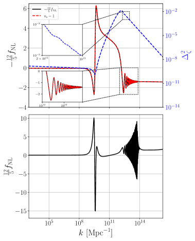
Figure 1: The primordial scalar power spectrum $\Delta_{\zeta}^{2}$ and the non-Gaussianity parameter $f_{\mathrm{NL}}$ for the G1 model (2.24) with the power-law potential $\lambda\phi^{2/5}$. The upper panel shows the power spectrum with the blue dashed line, $-\frac{12}{5}f_{\mathrm{NL}}$ in the squzeed limit with the solid black line for the modes $k_{1}=k_{2}=10^{6}k_{3}=k$ and the scalar spectral tilt $n_{\mathrm{s}}-1$ with the red dashed line. The insets show the oscillations in $\Delta_{\zeta}^{2}$ and $f_{\mathrm{NL}}$. The lower panel shows $\frac{12}{5}f_{\mathrm{NL}}$ in the equilateral limit for the modes $k_{1}=k_{2}=k_{3}=k$.

With Eqs. (2.13)-(2.23), we numerically compute the non-Gaussianity parameter $f_{\mathrm{NL}}$ in the squeezed limit and the equilateral limit. The results are shown in Fig. 1.

In the upper panel, we plot $-12f_{\mathrm{NL}}(k)/5$ along with the scalar spectral index $n_{\mathrm{s}}(k)-1$ to check the consistency relation

$$\lim_{k_{3}\rightarrow 0}f_{\mathrm{NL}}(k_{1},k_{2},k_{3})=\frac{5}{12}(1-n_{\mathrm{s}}),\quad\text{for}~{}k_{1}=k_{2}.$$ (2.25)

Our results confirm that the consistency relation (2.25) holds for models with peaks in the non-canonical kinetic term. The consistency relation which relates a three-point correlation function to a two-point correlation function, was derived originally in the canonical single-field inflation with slow roll [21]. Then it was proved to be true for any inflationary model as long as the inflaton is the only dynamical field in addition to the gravitational field during inflation [22]. From our results, we see that the non-Gaussianity parameter $f_{\text{NL}}$ can reach as large as order 1, at certain scales, $\left|12f_{\mathrm{NL}}\right|/5\simeq 6$ in the squeezed limit and $\left|12f_{\mathrm{NL}}\right|/5\simeq 15$ in the equilateral limit. Both maxima for $f_{\text{NL}}$ happen at the scales where the power spectrum has a small dip before it reaches the peak. For the model G1 considered in this subsection, there is a sharp spike for $f_{\text{NL}}$ at the scales between $k\sim 10^{9}~{}\mathrm{Mpc}^{-1}$ and $k\sim 10^{11}~{}\mathrm{Mpc}^{-1}$. The oscillation nature of $f_{\text{NL}}$ at scales around $k\sim 10^{13}~{}\mathrm{Mpc}^{-1}$ in both squeezed and equilateral limits originates from the small waggles in the power spectrum, as can be seen from the inset of Fig. 1. The oscillation in the power spectrum results in the oscillation in $f_{\mathrm{NL}}$ in the equilateral limit was also studied in Ref. [112].

If an inflationary model produces a power spectrum with a large slope, i.e., the power spectral $|n_{s}-1|\gg 1$, then the model has a large non-Gaussianity, at least in the squeezed limit, as told by the consistency relation (2.25) and shown in Fig. 1.

In terms of the nonlinear coupling constant $f_{\text{NL}}$ defined as [117, 20]

$$\zeta(\bm{x})=\zeta^{G}(\bm{x})+\frac{3}{5}f_{\text{NL}}(\zeta^{G}(\bm{x})^{2}-\langle\zeta^{G}(\bm{x})^{2}\rangle),$$ (2.26)

where $\zeta^{G}$ is the linear Gaussian part of the curvature perturbation, it was shown that the non-Gaussian contribution to SIGWs can exceed the Gaussian part if $\left(3/5\right)^{2}f^{2}_{\text{NL}}\Delta^{2}_{\zeta}\gtrsim 1$ [89]. Taking $f_{\mathrm{NL}}$ as the estimator to parameterize the magnitude of non-Gaussianity [25], we expect the contribution from the non-Gaussian scalar perturbations to SIGWs is negligible because $f_{\text{NL}}$ is small when the peak is reached as shown in Fig. 1.

The effect of non-Gaussianity of the curvature perturbation $\zeta$ on the PBH abundance is characterized by the factor $\mathcal{J}$ [118, 119, 120]

$$\mathcal{J}=\frac{1}{6\sigma^{3}_{R}}\int\frac{\mathrm{d}^{3}k_{1}}{(2\pi)^{3}}\int\frac{\mathrm{d}^{3}k_{2}}{(2\pi)^{3}}\int\frac{\mathrm{d}^{3}k_{3}}{(2\pi)^{3}}\mathrm{W}\left(k_{1}R\right)\mathrm{W}\left(k_{2}R\right)\mathrm{W}\left(k_{3}R\right)\left\langle\hat{\zeta}_{k_{1}}\hat{\zeta}_{k_{2}}\hat{\zeta}_{k_{3}}\right\rangle,$$ (2.27)

where the variance

$$\sigma_{R}^{2}=\int\frac{dk}{k}\mathrm{W}(kR)^{2}\Delta_{\zeta}^{2},$$ (2.28)

and $\mathrm{W}(kR)$ is a window function. If $\mathcal{J}\ll 1$, then the contribution of non-Gaussianity of the curvature perturbation to PBH abundance is negligible. Since the major contribution to $\mathcal{J}$ is around the peak of the power spectrum, for a good approximation we can use the value of $\mathcal{J}$ at the peak scale of the power spectrum of the curvature perturbation to evaluate the effect of non-Gaussianities on PBH abundance [120],

$$\mathcal{J}_{\mathrm{peak}}=\frac{3}{20\pi}f_{\mathrm{NL}}(k_{\mathrm{peak}},k_{\mathrm{peak}},k_{\mathrm{peak}})\sqrt{\Delta^{2}_{\zeta}(k_{\mathrm{peak}})}.$$ (2.29)

From Fig. 1, we see that $f_{\mathrm{NL}}(k_{\mathrm{peak}},k_{\mathrm{peak}},k_{\mathrm{peak}})\sim\mathcal{O}(1)$ and $\Delta^{2}_{\zeta}(k_{\mathrm{peak}})\sim\mathcal{O}(0.01)$. Plugging these numbers into Eq. (2.29), we obtain $\mathcal{J}_{\mathrm{peak}}\ll 1$, so we expect that the effect of non-Gaussianity on PBHs abundance is negligible.

2.3 G-inflation with Higgs field

For the G-inflation model G1 with the peak function (2.24) to be consistent with observational constraints, the potential is restricted to be $V(\phi)=\lambda\phi^{2/5}$. To lift the restriction on both the peak function and the inflationary potential, the non-canonical kinetic term in the model is generalized to [54, 55]

$$G(\phi)=G_{p}(\phi)+f(\phi),$$ (2.30)

where the peak function $G_{p}$ is generalized to

$$G_{p}(\phi)=\frac{d}{1+|(\phi-\phi_{p})/c|^{q}},$$ (2.31)

the function $f(\phi)$ is used to dress the non-canonical scalar field. It was shown that the enhanced power spectrum can have both sharp and broad peaks with the peak function (2.31). In this mechanism, Higgs inflation, T-model and natural inflation are shown to satisfy the observational constraints at large scales and the amplitudes of the power spectra are enhanced by seven orders of magnitude at small scales [54, 55, 56].

For the Higgs field with the potential $V(\phi)=\lambda\phi^{4}/4$, the function $f(\phi)$ is chosen to be [54, 55]

$$f(\phi)=f_{0}\phi^{22},$$ (2.32)

with $f_{0}$ a coupling constant. Following Ref. [55], we use H11 to represent the model with $q=1$, and H12 to represent the model with $q=5/4$. With the parameter settings as shown in Table. 2 [54, 55], we numerically compute the power spectrum $\Delta^{2}_{\zeta}$ and the non-Gaussianity parameters. We plot the results for the model H11 and the model H12 in Figs. 2 and 3, respectively.

Model	$q$	$d$	$c$	$\phi_{p}$	$\phi_{*}$	$f_{0}$	$\lambda$
H11	$1$	$1.05\times 10^{10}$	$2.04\times 10^{-10}$	$1.334$	$1.40$	$1$	$1.240\times 10^{-9}$
H12	$5/4$	$1.60\times 10^{11}$	$2.06\times 10^{-10}$	$1.300$	$1.40$	$1$	$1.244\times 10^{-9}$

Table 2: The parameters for the peak function (2.31) and the Higgs potential.

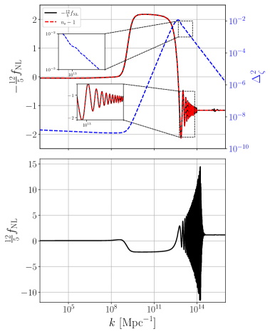
Figure 2: The primordial scalar power spectrum $\Delta_{\zeta}^{2}$ and the non-Gaussianity parameter $f_{\mathrm{NL}}$ for the Higgs model H11. The upper panel shows the power spectrum with the blue dashed line, $-\frac{12}{5}f_{\mathrm{NL}}$ in the squeezed limit with the solid black line for the modes $k_{1}=k_{2}=10^{6}k_{3}=k$ and the scalar spectral tilt $n_{\mathrm{s}}-1$ with the red dashed line. The insets show the oscillations in $\Delta_{\zeta}^{2}$ and $f_{\mathrm{NL}}$. The lower panel shows $\frac{12}{5}f_{\mathrm{NL}}$ in the equilateral limit for the modes $k_{1}=k_{2}=k_{3}=k$.

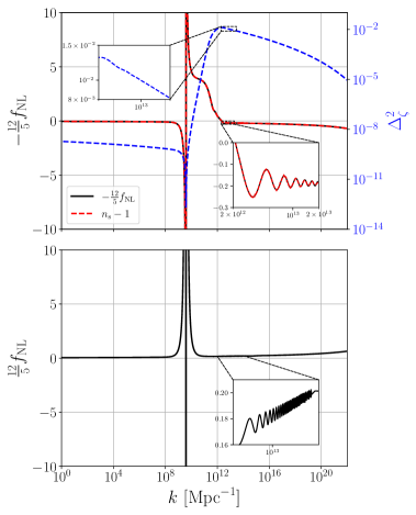
Figure 3: The primordial scalar power spectrum $\Delta_{\zeta}^{2}$ and the non-Gaussianity parameter $f_{\mathrm{NL}}$ for the Higgs model H12. The upper panel shows the power spectrum with the blue dashed line, $-\frac{12}{5}f_{\mathrm{NL}}$ in the squeezed limit with the solid black line for the modes $k_{1}=k_{2}=10^{6}k_{3}=k$ and the scalar spectral tilt $n_{\mathrm{s}}-1$ with the red dashed line. The insets show the oscillations in $\Delta_{\zeta}^{2}$ and $f_{\mathrm{NL}}$. The lower panel shows $\frac{12}{5}f_{\mathrm{NL}}$ in the equilateral limit for the modes $k_{1}=k_{2}=k_{3}=k$.

From the upper panels of Figs. 2 and 3, we see that the peak of the power spectrum produced by H12 is broader than that produced by H11, this is because the peak function $G_{p}(\phi)$ of the model H12 is flatter than H11.

In the upper panels of Figs. 2 and 3, we also plot the non-Gaussianity parameter $-12f_{\mathrm{NL}}/5$ in the squeezed limit along with the scalar spectral index $n_{\mathrm{s}}(k)-1$ to check the consistency relation (2.25). As shown in Figs. 2 and 3, the consistency relation still holds for models with either broad or sharp peaks in the non-canonical kinetic term, even when the slow roll conditions violate.

From Fig. 2, we see that in the model H11 with a sharp peak in the power spectrum, the non-Gaussianity parameter $f_{\mathrm{NL}}$ in the squeezed limit can be as large as $\left|12f_{\mathrm{NL}}/5\right|\simeq 2$ and $\left|12f_{\mathrm{NL}}/5\right|\simeq 15$ in the equilateral limit at certain scales. $f_{\mathrm{NL}}$ is almost a constant when the power spectrum climbs up to the peak. Due to the waggles in the power spectrum as shown in the insets of Fig. 2, $f_{\text{NL}}$ becomes large and it also shows the oscillation behaviour.

From Fig. 3, we see that $f_{\mathrm{{NL}}}$ has a pretty large value in the model H12 with a broad peak in the power spectrum at scales around $k\sim 10^{9}\ \text{Mpc}^{-1}$ due to the plunge by several orders of magnitude in the power spectrum, and the amplitude is about $10^{-14}$ at the relevant scales. However, $f_{\mathrm{NL}}$ is small at scales where the power spectrum reaches the peak. Again the waggles in the power spectrum as shown in the insets of Fig. 3 result in the oscillations in $f_{\mathrm{NL}}$.

Our numerical computations show that the three inflationary models predict different non-Gaussianities which could be taken as a tool to distinguish them. In general, there is much more information contained in the bispectrum than in the power spectrum. By virtue of non-Gaussianity, we may differentiate inflationary models when degeneracy happens.

For all these models, $f_{\mathrm{NL}}$ is small at the scales where the power spectrum reaches the peaks, so we don’t expect a large contribution from non-Gaussianity in the enhanced curvature perturbations to SIGWs and PBH abundance. Even large non-Gaussianities arise in the model H12, the contribution to SIGWs and PBH abundance is still negligible because the amplitudes of the perturbations are very small at those scales.

3 Conclusion

Non-Gaussianity is useful for understanding the dynamics of inflation and distinguishing different inflation models. We studied the non-Gaussianity of scalar perturbation produced in the G-inflation model with a peak function in the non-canonical kinetic term. The results confirm that the consistency relation holds in G-inflation models. Even though the peak function enhances the scalar power spectrum by seven orders of magnitude at small scales, the non-Gaussianity is small at the peak scales. For the model G1, $|12f_{\text{NL}}/5|$ can be as large as 6 in the squeezed limit and 15 in the equilateral limit. Because of the dip before the peak scale in the power spectrum for the model G1, $f_{\text{NL}}$ reaches its maximum value at the dip scale. The small waggles in the power spectrum not only result in the oscillation of $f_{\text{NL}}$, but also lead to large non-Gaussianity. For the Higgs model H11, $|12f_{\text{NL}}/5|$ is almost an order 1 constant in both squeezed and equilateral limits at scales where the power spectrum climbs up the peak. At the peak scale, $f_{\text{NL}}$ is small. After the peak, the small wiggles in the power spectrum lead to the oscillation of $|12f_{\text{NL}}/5|$ with the amplitude of order 2 in the squeezed limit and the amplitude of 15 in the equilateral limit. For the Higgs model H12, the power spectrum plunges by several orders of magnitude before it reaches the broad peak and the non-Gaussianity becomes very large at the plunge scales. However, $f_{\text{NL}}$ keeps to be small at the peak scales. Since $f_{\text{NL}}$ is small at the peak scales for all three models considered, the contributions of the non-Gaussianity of curvature perturbations to SIGWs and PBH abundance are negligible.

References

- [1] A. A. Starobinsky, A New Type of Isotropic Cosmological Models Without Singularity, Phys. Lett. B. 91 (1980) 99.
- [2] A. H. Guth, The Inflationary Universe: A Possible Solution to the Horizon and Flatness Problems, Phys. Rev. D 23 (1981) 347.
- [3] K. Sato, First Order Phase Transition of a Vacuum and Expansion of the Universe, Mon. Not. Roy. Astron. Soc. 195 (1981) 467.
- [4] A. D. Linde, A New Inflationary Universe Scenario: A Possible Solution of the Horizon, Flatness, Homogeneity, Isotropy and Primordial Monopole Problems, Phys. Lett. B 108 (1982) 389.
- [5] A. A. Starobinsky, Dynamics of Phase Transition in the New Inflationary Universe Scenario and Generation of Perturbations, Phys. Lett. B 117 (1982) 175.
- [6] A. Albrecht and P. J. Steinhardt, Cosmology for Grand Unified Theories with Radiatively Induced Symmetry Breaking, Phys. Rev. Lett. 48 (1982) 1220.
- [7] A. D. Linde, Chaotic Inflation, Phys. Lett. B 129 (1983) 177.
- [8] COBE collaboration, Structure in the COBE differential microwave radiometer first year maps, Astrophys. J. Lett. 396 (1992) L1.
- [9] WMAP collaboration, First year Wilkinson Microwave Anisotropy Probe (WMAP) observations: Determination of cosmological parameters, Astrophys. J. Suppl. 148 (2003) 175 [arXiv:astro-ph/0302209].
- [10] WMAP collaboration, Seven-Year Wilkinson Microwave Anisotropy Probe (WMAP) Observations: Cosmological Interpretation, Astrophys. J. Suppl. 192 (2011) 18 [arXiv:1001.4538].
- [11] Planck collaboration, Planck 2018 results. VI. Cosmological parameters, Astron. Astrophys. 641 (2020) A6 [arXiv:1807.06209].
- [12] Planck collaboration, Planck 2018 results. X. Constraints on inflation, Astron. Astrophys. 641 (2020) A10 [arXiv:1807.06211].
- [13] K. Sato and J. Yokoyama, Inflationary cosmology: First 30+ years, Int. J. Mod. Phys. D 24 (2015) 1530025.
- [14] BICEP2, Keck Array collaboration, BICEP2 / Keck Array x: Constraints on Primordial Gravitational Waves using Planck, WMAP, and New BICEP2/Keck Observations through the 2015 Season, Phys. Rev. Lett. 121 (2018) 221301 [arXiv:1810.05216].
- [15] X. Chen, Primordial Non-Gaussianities from Inflation Models, Adv. Astron. 2010 (2010) 638979 [arXiv:1002.1416].
- [16] N. Bartolo, E. Komatsu, S. Matarrese and A. Riotto, Non-Gaussianity from inflation: Theory and observations, Phys. Rept. 402 (2004) 103 [arXiv:astro-ph/0406398].
- [17] D. Seery and J. E. Lidsey, Primordial non-Gaussianities in single field inflation, JCAP 06 (2005) 003 [arXiv:astro-ph/0503692].
- [18] D. S. Salopek and J. R. Bond, Nonlinear evolution of long wavelength metric fluctuations in inflationary models, Phys. Rev. D 42 (1990) 3936.
- [19] A. Gangui, F. Lucchin, S. Matarrese and S. Mollerach, The Three point correlation function of the cosmic microwave background in inflationary models, Astrophys. J. 430 (1994) 447 [arXiv:astro-ph/9312033].
- [20] E. Komatsu and D. N. Spergel, Acoustic signatures in the primary microwave background bispectrum, Phys. Rev. D 63 (2001) 063002 [arXiv:astro-ph/0005036].
- [21] J. M. Maldacena, Non-Gaussian features of primordial fluctuations in single field inflationary models, JHEP 05 (2003) 013 [arXiv:astro-ph/0210603].
- [22] P. Creminelli and M. Zaldarriaga, Single field consistency relation for the 3-point function, JCAP 10 (2004) 006 [arXiv:astro-ph/0407059].
- [23] P. Creminelli, A. Nicolis, L. Senatore, M. Tegmark and M. Zaldarriaga, Limits on non-gaussianities from wmap data, JCAP 05 (2006) 004 [arXiv:astro-ph/0509029].
- [24] P. Creminelli, L. Senatore, M. Zaldarriaga and M. Tegmark, Limits on f_NL parameters from WMAP 3yr data, JCAP 03 (2007) 005 [arXiv:astro-ph/0610600].
- [25] X. Chen, M.-X. Huang, S. Kachru and G. Shiu, Observational signatures and non-Gaussianities of general single field inflation, JCAP 01 (2007) 002 [arXiv:hep-th/0605045].
- [26] V. Sreenath, D. K. Hazra and L. Sriramkumar, On the scalar consistency relation away from slow roll, JCAP 02 (2015) 029 [arXiv:1410.0252].
- [27] A. De Felice and S. Tsujikawa, Inflationary non-Gaussianities in the most general second-order scalar-tensor theories, Phys. Rev. D 84 (2011) 083504 [arXiv:1107.3917].
- [28] T. Kobayashi, M. Yamaguchi and J. Yokoyama, Primordial non-Gaussianity from G-inflation, Phys. Rev. D 83 (2011) 103524 [arXiv:1103.1740].
- [29] A. De Felice and S. Tsujikawa, Primordial non-Gaussianities in general modified gravitational models of inflation, JCAP 04 (2011) 029 [arXiv:1103.1172].
- [30] Planck collaboration, Planck 2018 results. IX. Constraints on primordial non-Gaussianity, Astron. Astrophys. 641 (2020) A9 [arXiv:1905.05697].
- [31] H. Di and Y. Gong, Primordial black holes and second order gravitational waves from ultra-slow-roll inflation, JCAP 07 (2018) 007 [arXiv:1707.09578].
- [32] J. Garcia-Bellido and E. Ruiz Morales, Primordial black holes from single field models of inflation, Phys. Dark Univ. 18 (2017) 47 [arXiv:1702.03901].
- [33] C. Germani and T. Prokopec, On primordial black holes from an inflection point, Phys. Dark Univ. 18 (2017) 6 [arXiv:1706.04226].
- [34] H. Motohashi and W. Hu, Primordial Black Holes and Slow-Roll Violation, Phys. Rev. D 96 (2017) 063503 [arXiv:1706.06784].
- [35] J. M. Ezquiaga, J. Garcia-Bellido and E. Ruiz Morales, Primordial Black Hole production in Critical Higgs Inflation, Phys. Lett. B 776 (2018) 345 [arXiv:1705.04861].
- [36] F. Bezrukov, M. Pauly and J. Rubio, On the robustness of the primordial power spectrum in renormalized Higgs inflation, JCAP 02 (2018) 040 [arXiv:1706.05007].
- [37] J. R. Espinosa, D. Racco and A. Riotto, Cosmological Signature of the Standard Model Higgs Vacuum Instability: Primordial Black Holes as Dark Matter, Phys. Rev. Lett. 120 (2018) 121301 [arXiv:1710.11196].
- [38] G. Ballesteros and M. Taoso, Primordial black hole dark matter from single field inflation, Phys. Rev. D 97 (2018) 023501 [arXiv:1709.05565].
- [39] G. Ballesteros, J. Beltran Jimenez and M. Pieroni, Black hole formation from a general quadratic action for inflationary primordial fluctuations, JCAP 06 (2019) 016 [arXiv:1811.03065].
- [40] M. Sasaki, T. Suyama, T. Tanaka and S. Yokoyama, Primordial black holes—perspectives in gravitational wave astronomy, Class. Quant. Grav. 35 (2018) 063001 [arXiv:1801.05235].
- [41] A. Y. Kamenshchik, A. Tronconi, T. Vardanyan and G. Venturi, Non-Canonical Inflation and Primordial Black Holes Production, Phys. Lett. B 791 (2019) 201 [arXiv:1812.02547].
- [42] T.-J. Gao and Z.-K. Guo, Primordial Black Hole Production in Inflationary Models of Supergravity with a Single Chiral Superfield, Phys. Rev. D 98 (2018) 063526 [arXiv:1806.09320].
- [43] I. Dalianis, A. Kehagias and G. Tringas, Primordial black holes from -attractors, JCAP 01 (2019) 037 [arXiv:1805.09483].
- [44] I. Dalianis, S. Karydas and E. Papantonopoulos, Generalized Non-Minimal Derivative Coupling: Application to Inflation and Primordial Black Hole Production, JCAP 06 (2020) 040 [arXiv:1910.00622].
- [45] S. Passaglia, W. Hu and H. Motohashi, Primordial black holes and local non-Gaussianity in canonical inflation, Phys. Rev. D 99 (2019) 043536 [arXiv:1812.08243].
- [46] G. Ballesteros, J. Rey and F. Rompineve, Detuning primordial black hole dark matter with early matter domination and axion monodromy, JCAP 06 (2020) 014 [arXiv:1912.01638].
- [47] S. Passaglia, W. Hu and H. Motohashi, Primordial black holes as dark matter through Higgs field criticality, Phys. Rev. D 101 (2020) 123523 [arXiv:1912.02682].
- [48] C. Fu, P. Wu and H. Yu, Primordial Black Holes from Inflation with Nonminimal Derivative Coupling, Phys. Rev. D 100 (2019) 063532 [arXiv:1907.05042].
- [49] C. Fu, P. Wu and H. Yu, Scalar induced gravitational waves in inflation with gravitationally enhanced friction, Phys. Rev. D 101 (2020) 023529 [arXiv:1912.05927].
- [50] W.-T. Xu, J. Liu, T.-J. Gao and Z.-K. Guo, Gravitational waves from double-inflection-point inflation, Phys. Rev. D 101 (2020) 023505 [arXiv:1907.05213].
- [51] M. Braglia, D. K. Hazra, F. Finelli, G. F. Smoot, L. Sriramkumar and A. A. Starobinsky, Generating PBHs and small-scale GWs in two-field models of inflation, JCAP 08 (2020) 001 [arXiv:2005.02895].
- [52] A. Gundhi and C. F. Steinwachs, Scalaron-Higgs inflation reloaded: Higgs-dependent scalaron mass and primordial black hole dark matter, arXiv:2011.09485.
- [53] J. Lin, Q. Gao, Y. Gong, Y. Lu, C. Zhang and F. Zhang, Primordial black holes and secondary gravitational waves from and inflation, Phys. Rev. D 101 (2020) 103515 [arXiv:2001.05909].
- [54] Z. Yi, Y. Gong, B. w and Z.-h. Zhu, Primordial black holes and secondary gravitational waves from the Higgs field, Phys. Rev. D 103 (2021) 063535 [arXiv:2007.09957].
- [55] Z. Yi, Q. Gao, Y. Gong, and Z.-h. Zhu, Primordial black holes and scalar-induced secondary gravitational waves from inflationary models with a noncanonical kinetic term, Phys. Rev. D 103 (2021) 063534 [arXiv:2011.10606].
- [56] Q. Gao, Y. Gong and Z. Yi, Primordial black holes and secondary gravitational waves from natural inflation, arXiv:2012.03856.
- [57] J. Fumagalli, S. Renaux-Petel, J. W. Ronayne and L. T. Witkowski, Turning in the landscape: a new mechanism for generating Primordial Black Holes, arXiv:2004.08369.
- [58] J. Fumagalli, S. Renaux-Petel and L. T. Witkowski, Oscillations in the stochastic gravitational wave background from sharp features and particle production during inflation, arXiv:2012.02761.
- [59] A. Gundhi, S. V. Ketov and C. F. Steinwachs, Primordial black hole dark matter in dilaton-extended two-field Starobinsky inflation, arXiv:2011.05999.
- [60] G. Ballesteros, J. Rey, M. Taoso and A. Urbano, Primordial black holes as dark matter and gravitational waves from single-field polynomial inflation, JCAP 07 (2020) 025 [arXiv:2001.08220].
- [61] H. V. Ragavendra, P. Saha, L. Sriramkumar and J. Silk, PBHs and secondary GWs from ultra slow roll and punctuated inflation, arXiv:2008.12202.
- [62] B. J. Carr and S. W. Hawking, Black holes in the early Universe, Mon. Not. Roy. Astron. Soc. 168 (1974) 399.
- [63] S. Hawking, Gravitationally collapsed objects of very low mass, Mon. Not. Roy. Astron. Soc. 152 (1971) 75.
- [64] P. Ivanov, P. Naselsky and I. Novikov, Inflation and primordial black holes as dark matter, Phys. Rev. D 50 (1994) 7173.
- [65] P. H. Frampton, M. Kawasaki, F. Takahashi and T. T. Yanagida, Primordial Black Holes as All Dark Matter, JCAP 04 (2010) 023 [arXiv:1001.2308].
- [66] K. M. Belotsky, A. D. Dmitriev, E. A. Esipova, V. A. Gani, A. V. Grobov, M. Y. Khlopov et al., Signatures of primordial black hole dark matter, Mod. Phys. Lett. A 29 (2014) 1440005 [arXiv:1410.0203].
- [67] M. Y. Khlopov, S. G. Rubin and A. S. Sakharov, Primordial structure of massive black hole clusters, Astropart. Phys. 23 (2005) 265 [arXiv:astro-ph/0401532].
- [68] S. Clesse and J. García-Bellido, Massive Primordial Black Holes from Hybrid Inflation as Dark Matter and the seeds of Galaxies, Phys. Rev. D 92 (2015) 023524 [arXiv:1501.07565].
- [69] B. Carr, F. Kuhnel and M. Sandstad, Primordial Black Holes as Dark Matter, Phys. Rev. D 94 (2016) 083504 [arXiv:1607.06077].
- [70] S. Pi, Y.-L. Zhang, Q.-G. Huang and M. Sasaki, Scalaron from -gravity as a heavy field, JCAP 05 (2018) 042 [arXiv:1712.09896].
- [71] K. Inomata, M. Kawasaki, K. Mukaida, Y. Tada and T. T. Yanagida, Inflationary Primordial Black Holes as All Dark Matter, Phys. Rev. D 96 (2017) 043504 [arXiv:1701.02544].
- [72] J. García-Bellido, Massive Primordial Black Holes as Dark Matter and their detection with Gravitational Waves, J. Phys. Conf. Ser. 840 (2017) 012032 [arXiv:1702.08275].
- [73] E. D. Kovetz, Probing Primordial-Black-Hole Dark Matter with Gravitational Waves, Phys. Rev. Lett. 119 (2017) 131301 [arXiv:1705.09182].
- [74] B. Carr and F. Kuhnel, Primordial Black Holes as Dark Matter: Recent Developments, Ann. Rev. Nucl. Part. Sci. 70 (2020) 355 [arXiv:2006.02838].
- [75] S. Matarrese, S. Mollerach and M. Bruni, Second order perturbations of the Einstein-de Sitter universe, Phys. Rev. D 58 (1998) 043504 [arXiv:astro-ph/9707278].
- [76] S. Mollerach, D. Harari and S. Matarrese, CMB polarization from secondary vector and tensor modes, Phys. Rev. D 69 (2004) 063002 [arXiv:astro-ph/0310711].
- [77] K. N. Ananda, C. Clarkson and D. Wands, The Cosmological gravitational wave background from primordial density perturbations, Phys. Rev. D 75 (2007) 123518 [arXiv:gr-qc/0612013].
- [78] D. Baumann, P. J. Steinhardt, K. Takahashi and K. Ichiki, Gravitational Wave Spectrum Induced by Primordial Scalar Perturbations, Phys. Rev. D 76 (2007) 084019 [arXiv:hep-th/0703290].
- [79] J. Garcia-Bellido, M. Peloso and C. Unal, Gravitational Wave signatures of inflationary models from Primordial Black Hole Dark Matter, JCAP 09 (2017) 013 [arXiv:1707.02441].
- [80] R. Saito and J. Yokoyama, Gravitational wave background as a probe of the primordial black hole abundance, Phys. Rev. Lett. 102 (2009) 161101 [arXiv:0812.4339].
- [81] R. Saito and J. Yokoyama, Gravitational-Wave Constraints on the Abundance of Primordial Black Holes, Prog. Theor. Phys. 123 (2010) 867 [arXiv:0912.5317].
- [82] E. Bugaev and P. Klimai, Induced gravitational wave background and primordial black holes, Phys. Rev. D 81 (2010) 023517 [arXiv:0908.0664].
- [83] E. Bugaev and P. Klimai, Constraints on the induced gravitational wave background from primordial black holes, Phys. Rev. D 83 (2011) 083521 [arXiv:1012.4697].
- [84] L. Alabidi, K. Kohri, M. Sasaki and Y. Sendouda, Observable Spectra of Induced Gravitational Waves from Inflation, JCAP 09 (2012) 017 [arXiv:1203.4663].
- [85] N. Orlofsky, A. Pierce and J. D. Wells, Inflationary theory and pulsar timing investigations of primordial black holes and gravitational waves, Phys. Rev. D 95 (2017) 063518 [arXiv:1612.05279].
- [86] T. Nakama, J. Silk and M. Kamionkowski, Stochastic gravitational waves associated with the formation of primordial black holes, Phys. Rev. D 95 (2017) 043511 [arXiv:1612.06264].
- [87] K. Inomata, M. Kawasaki, K. Mukaida, Y. Tada and T. T. Yanagida, Inflationary primordial black holes for the LIGO gravitational wave events and pulsar timing array experiments, Phys. Rev. D 95 (2017) 123510 [arXiv:1611.06130].
- [88] S.-L. Cheng, W. Lee and K.-W. Ng, Primordial black holes and associated gravitational waves in axion monodromy inflation, JCAP 07 (2018) 001 [arXiv:1801.09050].
- [89] R.-G. Cai, S. Pi and M. Sasaki, Gravitational Waves Induced by non-Gaussian Scalar Perturbations, Phys. Rev. Lett. 122 (2019) 201101 [arXiv:1810.11000].
- [90] N. Bartolo, V. De Luca, G. Franciolini, M. Peloso, D. Racco and A. Riotto, Testing primordial black holes as dark matter with LISA, Phys. Rev. D 99 (2019) 103521 [arXiv:1810.12224].
- [91] N. Bartolo, V. De Luca, G. Franciolini, A. Lewis, M. Peloso and A. Riotto, Primordial Black Hole Dark Matter: LISA Serendipity, Phys. Rev. Lett. 122 (2019) 211301 [arXiv:1810.12218].
- [92] K. Kohri and T. Terada, Semianalytic calculation of gravitational wave spectrum nonlinearly induced from primordial curvature perturbations, Phys. Rev. D 97 (2018) 123532 [arXiv:1804.08577].
- [93] J. R. Espinosa, D. Racco and A. Riotto, A Cosmological Signature of the SM Higgs Instability: Gravitational Waves, JCAP 09 (2018) 012 [arXiv:1804.07732].
- [94] S. Kuroyanagi, T. Chiba and T. Takahashi, Probing the Universe through the Stochastic Gravitational Wave Background, JCAP 11 (2018) 038 [arXiv:1807.00786].
- [95] R.-G. Cai, S. Pi, S.-J. Wang and X.-Y. Yang, Resonant multiple peaks in the induced gravitational waves, JCAP 05 (2019) 013 [arXiv:1901.10152].
- [96] R.-G. Cai, S. Pi, S.-J. Wang and X.-Y. Yang, Pulsar Timing Array Constraints on the Induced Gravitational Waves, JCAP 10 (2019) 059 [arXiv:1907.06372].
- [97] R.-G. Cai, Z.-K. Guo, J. Liu, L. Liu and X.-Y. Yang, Primordial black holes and gravitational waves from parametric amplification of curvature perturbations, JCAP 06 (2020) 013 [arXiv:1912.10437].
- [98] R.-G. Cai, Y.-C. Ding, X.-Y. Yang and Y.-F. Zhou, Constraints on a mixed model of dark matter particles and primordial black holes from the galactic 511 keV line, JCAP 03 (2021) 057 [arXiv:2007.11804].
- [99] G. Domènech, Induced gravitational waves in a general cosmological background, Int. J. Mod. Phys. D 29 (2020) 2050028 [arXiv:1912.05583].
- [100] M. Drees and Y. Xu, Overshooting, Critical Higgs Inflation and Second Order Gravitational Wave Signatures, Eur. Phys. J. C 81(2021)182 [arXiv:1905.13581].
- [101] K. Inomata, K. Kohri, T. Nakama and T. Terada, Enhancement of Gravitational Waves Induced by Scalar Perturbations due to a Sudden Transition from an Early Matter Era to the Radiation Era, Phys. Rev. D 100 (2019) 043532 [arXiv:1904.12879].
- [102] K. Inomata, K. Kohri, T. Nakama and T. Terada, Gravitational Waves Induced by Scalar Perturbations during a Gradual Transition from an Early Matter Era to the Radiation Era, JCAP 10 (2019) 071 [arXiv:1904.12878].
- [103] V. De Luca, V. Desjacques, G. Franciolini and A. Riotto, Gravitational Waves from Peaks, JCAP 09 (2019) 059 [arXiv:1905.13459].
- [104] G. Domènech, S. Pi and M. Sasaki, Induced gravitational waves as a probe of thermal history of the universe, JCAP 08 (2020) 017 [arXiv:2005.12314].
- [105] M. Braglia, X. Chen and D. K. Hazra, Probing Primordial Features with the Stochastic Gravitational Wave Background, JCAP 03 (2021) 005 [arXiv:2012.05821].
- [106] T. Kobayashi, M. Yamaguchi and J. Yokoyama, G-inflation: Inflation driven by the Galileon field, Phys. Rev. Lett. 105 (2010) 231302 [arXiv:1008.0603].
- [107] T. Kobayashi, M. Yamaguchi and J. Yokoyama, Generalized G-inflation: Inflation with the most general second-order field equations, Prog. Theor. Phys. 126 (2011) 511 [arXiv:1105.5723].
- [108] V. F. Mukhanov, Gravitational Instability of the Universe Filled with a Scalar Field, JETP Lett. 41 (1985) 493.
- [109] M. Sasaki, Large Scale Quantum Fluctuations in the Inflationary Universe, Prog. Theor. Phys. 76 (1986) 1036.
- [110] C. T. Byrnes, M. Gerstenlauer, S. Nurmi, G. Tasinato and D. Wands, Scale-dependent non-Gaussianity probes inflationary physics, JCAP 10 (2010) 004 [arXiv:1007.4277].
- [111] Planck collaboration, Planck 2015 results. XVII. Constraints on primordial non-Gaussianity, Astron. Astrophys. 594 (2016) A17 [arXiv:1502.01592].
- [112] D. K. Hazra, L. Sriramkumar and J. Martin, BINGO: A code for the efficient computation of the scalar bi-spectrum, JCAP 05 (2013) 026 [arXiv:1201.0926].
- [113] H. V. Ragavendra, D. Chowdhury and L. Sriramkumar, Suppression of scalar power on large scales and associated bispectra, arXiv:2003.01099.
- [114] F. Arroja and T. Tanaka, A note on the role of the boundary terms for the non-Gaussianity in general k-inflation, JCAP 05 (2011) 005 [arXiv:1103.1102].
- [115] X. Chen, R. Easther and E. A. Lim, Large Non-Gaussianities in Single Field Inflation, JCAP 06 (2007) 023 [arXiv:astro-ph/0611645].
- [116] X. Chen, R. Easther and E. A. Lim, Generation and Characterization of Large Non-Gaussianities in Single Field Inflation, JCAP 04 (2008) 010 [arXiv:0801.3295].
- [117] L. Verde, L.-M. Wang, A. Heavens and M. Kamionkowski, Large scale structure, the cosmic microwave background, and primordial non-gaussianity, Mon. Not. Roy. Astron. Soc. 313 (2000) L141 [arXiv:astro-ph/9906301].
- [118] D. Seery and J. C. Hidalgo, Non-Gaussian corrections to the probability distribution of the curvature perturbation from inflation, JCAP 07 (2006) 008 [arXiv:astro-ph/0604579].
- [119] J. C. Hidalgo, The effect of non-Gaussian curvature perturbations on the formation of primordial black holes, arXiv:0708.3875.
- [120] R. Saito, J. Yokoyama and R. Nagata, Single-field inflation, anomalous enhancement of superhorizon fluctuations, and non-Gaussianity in primordial black hole formation, JCAP 06 (2008) 024 [arXiv:0804.3470].