Open-World Class Discovery with Kernel Networks

Abstract

We study an Open-World Class Discovery problem in which, given labeled training samples from old classes, we need to discover new classes from unlabeled test samples. There are two critical challenges to addressing this paradigm: (a) transferring knowledge from old to new classes, and (b) incorporating knowledge learned from new classes back to the original model. We propose Class Discovery Kernel Network with Expansion (CD-KNet-Exp), a deep learning framework, which utilizes the Hilbert Schmidt Independence Criterion to bridge supervised and unsupervised information together in a systematic way, such that the learned knowledge from old classes is distilled appropriately for discovering new classes. Compared to competing methods, CD-KNet-Exp shows superior performance on three publicly available benchmark datasets and a challenging real-world radio frequency fingerprinting dataset.

I Introduction

In the conventional supervised learning setting, we assume that we know all classes in advance; i.e., the classes that appear in the test set will be a subset of classes in the training set. This has been termed as the closed-world assumption [1, 2]; recent advances in deep learning [3] have given impressive performance on supervised learning problems where the closed-world assumption holds, such as computer vision [4, 5] and natural language processing [6]. However, in real world applications, we often encounter an open-world [2, 7, 8] setting, in which unlabeled test samples come from new, previously unseen classes. This would be the case when a trained classifier is deployed in a completely new environment.

As a concrete example, consider a classifier that has been trained to distinguish between different breeds of dogs. An open-world class discovery problem would arise if we had access to this trained classifier, and we ask to classify a wholly different test set, containing, e.g., different breeds of cats. Ideally, we would like to somehow leverage the dog classifier to distinguish between cat breeds. Though clearly, we cannot name cat breeds in this setting, it is possible that, by incorporating the knowledge learned from dogs, we would be able to discover the new cat breeds, clustering samples from the same breeds together.

This problem constitutes the open-world class discovery problem [9, 10]. Open-world class discovery poses a significant challenge, as transferring learned knowledge on old classes to new classes is not straightforward. Machine learning models may overfit to old classes; as a result, knowledge learned, particularly through latent representations, may not generalize well to new classes. The more dissimilar old and new classes are, the more pronounced this problem becomes. Identifying which knowledge to transfer and leverage from old classes when trying to discover new classes is not trivial. This is further exacerbated in the case of deep models, that are by nature less interpretable. Coming up with an automated, principled way of extracting commonalities among representations is the main obstacle behind open-world settings.

We address these challenges via an algorithm for leveraging deep architectures to solve the open-world class discovery problem. We first train a classifier on known classes. We subsequently retrain it in the presence of unlabeled samples of new, previously unseen classes using an objective based on the Hilbert Schmidt Independence Criterion (HSIC). Intuitively, our scheme fine-tunes the latent representation obtained over the old-class dataset so that, when used to map new-class samples, the resulting images span a low rank subspace and are (jointly) well-clusterable. This is accomplished even for deep models, whose latent representation is difficult to interpret.

Formally, our contributions are as follows:

• We propose a deep learning framework which utilizes HSIC to bridge supervised and unsupervised information together in a systematic way, so that learned knowledge from old classes is distilled appropriately for new classes. Our approach addresses overfitting to old classes, leading to improved class discovery, and can be generically applied to a broad array of deep architectures.

• Our algorithm, CD-KNet-Exp, shows superior performance on three benchmark datasets, including MNIST, Fashion-MNIST, CIFAR-100, and also a real world radio frequency fingerprinting dataset. In particular, it outperforms competitors over three benchmark datasets by a $2\%$-$12\%$ margin.

The rest of this paper is organized as follows. We present related work in Section II. Next, in Section III, we formally define the open world class discovery problem and introduce our notation. We give an overview of HSIC and its uses for supervised and unsupervised learning in Section IV. In Section V, we present our three-stage framework in detail. Our experimental results are provided in Section VII; finally, we conclude in Section VIII.

II Related Work

Novelty Detection. A large body of prior work has been focused on novelty detection [11, 12], where the task is to design a model capable of both classifying instances that belong to the known training classes, and detect instances belonging to novel emerging classes at the same time. This differs from our setting, as the goal is to detect from a mixture of old and new samples which ones are old and which ones are new, without clustering the latter. Recently, a number of novelty detection methods were proposed based on kernel density estimation [13, 14], nearest neighbor [15, 16, 17] and recent advances in deep learning [18, 19]. Our setting is orthogonal/complementary: once novel samples are detected, our method can be applied to discover new classes.

Semi-Supervised Learning. Our problem setting seems close to semi-supervised learning [20, 21], where some samples are labeled and others are not. However, in semi-supervised classification problem, all classes are known and every class has a corresponding labeled portion: some of the samples for each class are labeled and the others are unlabeled. Information transfer can be achieved via deep learning models with great representational power [22, 23]. Additional information provided on the samples can be leveraged [24, 25], such as must-link and cannot-link constraints. In contrast, our task aims to discover unseen new classes with no direct constraint information about these unseen new classes. All the knowledge we have comes from the labeled old classes. Hence, in the open-world class discovery problem, figuring out how to transfer knowledge learned from old classes to new classes is a critical challenge that needs to be addressed.

Open-World Class Discovery. To the best of our knowledge, very limited research has been performed in the area of class discovery. Recently, Nixon et al. [10] proposed to train a neural network classifier on old classes, followed by applying the K-means [26] algorithm to directly cluster the new classes on the features extracted by the trained network. They provide two strategies for adding the new discovered classes back to the classifier: static, where all new classes are added at once; and dynamic, where a single, most appropriate, class is added. Shu et al. [9] use a pairwise network to learn a proper distance metric from seen old classes and utilize that metric for clustering the unsupervised data to discover new classes. Nixon et al. [10] use a feature extractor that is trained only on the seen old classes. Similarly, Shu et al. [9] train their distance metric only on the seen old classes. Training only on the old classes may not be appropriate for the new classes. CD-KNet, on the other hand, discovers new classes by learning a feature extractor that leverages information from both supervised seen old classes and the unsupervised data.

III Open World Class Discovery

In this section, we provide a precise formulation of the open world class discovery problem; Table I summarizes our notation. First, we are given a labeled dataset $\mathcal{D}_{l}=\{({x}_{i},y_{i})\}_{i=1}^{n}$, where ${x}_{i}\in\mathbb{R}^{d_{0}}$ is the input sample and $y_{i}\in\mathcal{L}$ is the class label, from $m_{l}=|\mathcal{L}|$ classes. We are also given an unlabeled dataset $\mathcal{D}_{u}=\{{x}_{j}\}_{j=1}^{n^{\prime}}$, where ${x}_{j}\in\mathbb{R}^{d_{0}}$. These unlabeled samples belong to wholly distinct new classes, that are not present in $\mathcal{D}_{l}$. That is, each sample $x_{j}\in\mathcal{D}_{u}$ is associated with class label $y_{j}\in\mathcal{L}^{\prime}$, where $\mathcal{L}^{\prime}$ is again a finite set of size $m_{u}=|\mathcal{L}^{\prime}|$ such that $\mathcal{L}\cap\mathcal{L}^{\prime}=\emptyset$. Our goal is to (a) train a classifier on $\mathcal{D}_{l}$, and (b) leverage it over $\mathcal{D}_{u}$, so that we can discover (latent) ground truth classes in $\mathcal{D}_{u}$. Of course, $\mathcal{L}^{\prime}$ cannot be discovered per se. Our objective is to therefore more precisely stated as clustering groups of $x_{j}\in\mathcal{D}_{u}$ if they share the same (unseen) label in $\mathcal{L}^{\prime}$. We assume that the number of new classes $m_{u}$ is known.

Note that we have made two assumptions: (a) unlabeled samples only come from new classes and (b) the number of new classes are known. We can relax the first assumption, for example, by applying a novelty detector first to filter out old classes (see, e.g., [11, 27]). Moreover, we can discover $m_{u}$ through standard methods from clustering literature (see, e.g., [28]).

TABLE I: Notation Summary

Notation	Description
$\mathcal{D}_{l}$	A labeled dataset
$x_{i}$	Input sample $i$ from $\mathcal{D}_{l}$
$y_{i}$	Corresponding label of sample $i$ from $\mathcal{D}_{l}$
$n$	Number of samples in the labeled dataset $\mathcal{D}_{l}$
$\mathcal{L}$	Set of known labels
$m_{l}$	Cardinality of set $\mathcal{L}$ (number of old classes)
$\mathcal{D}_{u}$	An unlabeled dataset
$x_{j}$	Input sample $j$ from $\mathcal{D}_{u}$
${n}^{\prime}$	Number of samples in the unlabeled dataset $\mathcal{D}_{u}$
$\mathcal{L}^{\prime}$	Set of new classes
$m_{u}$	Cardinality of set $\mathcal{L^{\prime}}$ ( number of new classes)
$d_{0}$	Dimension of input samples $x_{i}$, $x_{j}$
$K_{P}$	Kernel matrix of input samples matrix $P$
$K_{Q}$	Kernel matrix of labels matrix $Q$
$\mathbb{H}(P,Q)$	Hilbert Schmidt Independence Criterion between two
	datasets, $P$ and $Q$ – Eq. (3)
$\text{tr}(\cdot)$	Trace of a matrix
$\theta$	Parameter of feature extractor
$f_{\theta}(X)$	Latent feature embedding of data $X$ parametrized by $\theta$
$d$	Reduced dimension after applying feature extractor
$X_{l}$	Data matrix of labeled dataset $\mathcal{D}_{l}$
$X_{u}$	Data matrix of unlabeled dataset $\mathcal{D}_{u}$
$Y$	Label matrix of labeled dataset $\mathcal{D}_{l}$
$X$	Data matrix of both labeled and unlabeled datasets
$U$	latent emebeding of $X$
$\mathbb{H}_{o}$	CD-KNet objective (Eq. (9))
$\lambda$	Control parameter in Eq. (9)
$\hat{y}_{j}$	Pseudo-labels/cluster assignments for ${n}^{\prime}$ samples
$\gamma$	Learning rate
$D$	Degree matrix (Eq. (6))
$n_{1}$	Number of samples from $\mathcal{D}_{l}$ used in computing $\mathbb{H}_{o}$
$n_{1}^{\prime}$	Number of samples from $\mathcal{D}_{u}$ used in computing $\mathbb{H}_{o}$

IV Hilbert Schmidt Independence Criterion

The Hilbert Schmidt Independence Criterion (HSIC) [29] is a statistical dependence measure between two random variables. Just like Mutual Information (MI), it captures non-linear dependencies between the random variables. Compared to MI, its empirical computation is easy, avoiding the explicit estimation of joint probability distributions. On account of this, it has been widely applied in different domains, such as feature selection [30], dimensionality reduction [31], alternative clustering [32], and deep clustering [33].

Formally, consider a set of i.i.d. sample tuples $\{(p_{i},q_{i})\}_{i=1}^{N}$, where $p_{i}\in\mathbb{R}^{d}$, $q_{i}\in\mathbb{R}^{c}$. Let $P\in\mathbb{R}^{N\times d}$ and $Q\in\mathbb{R}^{N\times c}$ be the matrices whose rows are the corresponding samples. Also, let $k_{p}:\mathbb{R}^{d}\times\mathbb{R}^{d}\rightarrow\mathbb{R}$ and $k_{q}:\mathbb{R}^{c}\times\mathbb{R}^{c}\rightarrow\mathbb{R}$ be two characteristic kernel functions for $p_{i}$ and $q_{i}$, respectively. Examples are

$$k_{P}(p_{i},p_{j})=e^{-\frac{\|p_{i}-p_{j},\|^{2}}{2\sigma^{2}}}$$ (1)

i.e., the Gaussian kernel, and the linear kernel

$$k_{Q}(q_{i},q_{j})=q_{i}^{\top}q_{j}.$$ (2)

We further define $K_{P},K_{Q}$ to be the kernel matrices for $P$ and $Q$ respectively, where $K_{P}=\{k_{P}(p_{i},p_{j})\}_{i,j}\in\mathbb{R}^{N\times N}$ and $K_{Q}=\{k_{Q}(q_{i},q_{j})\}_{i,j}\in\mathbb{R}^{N\times N}$.

The HSIC between $P$ and $Q$ is estimated empirically with kernels $k_{P},k_{Q}$ via:

$$\mathbb{H}(P,Q)=\frac{1}{(N-1)^{2}}\text{tr}(K_{P}HK_{Q}H),$$ (3)

where $H_{i,j}=\delta_{i,j}-N^{-1}$. Intuitively, HSIC measures the dependence between the random variables $p,q$ from which the i.i.d. samples $\{(p_{i},q_{i})\}_{i=1}^{N}$ where generated.

IV-A Supervised learning setting

Consider a data matrix $X\in\mathbb{R}^{N\times d_{0}}$, containing $N$ $d_{0}$-dimensional samples per row, and label matrix $Y\in\{0,1\}^{N\times m}$, representing the one-hot encoding of $m$ labels. We can utilize HSIC to perform dimensionality reduction in this supervised learning setting [34]. We can do so by maximizing the dependency between a non-linear feature mapping of input $X$ and labels $Y$ as follows. Let $f:\mathbb{R}^{d_{0}}\mapsto\mathbb{R}^{d}$, where $d\ll d_{0}$, be a feature extractor, e.g. neural network, parameterized by $\theta$. Denote by $f(X)\in\mathbb{R}^{N\times d}$ the matrix of images of rows (i.e., samples) in $X$. We can substitute $f_{\theta}(X),Y$ for $P,Q$ in Eq. (3), We set $K_{X}$ as a Gaussian kernel and $K_{Y}$ as a linear kernel. Then the solution of the following optimization problem:

$$\underset{\theta}{\operatorname{max}} \quad\mathbb{H}(f_{\theta}(X),Y),$$ (4)

maximizes the dependence of $f_{\theta}(X)$ and $Y$. Intuitively, this forces the feature extractor to be maximally correlated with $Y$. Having reduced dimensions thusly, a shallow classifier (e.g., logistic regression) can be used to learn the labels from the lower dimensional images $f_{\theta}(X)$.

IV-B Unsupervised learning setting

In the unsupervised case, we are only given data matrix $X\in\mathbb{R}^{N\times d_{0}}$. We can utilize HSIC to perform unsupervised learning by maximizing the dependency between a non-linear feature mapping of input $X$ and a learnable latent cluster embedding matrix $U\in\mathbb{R}^{N\times c}$ (see [33, 31]). We substitute $P,Q$ with $X,U$. Under the unsupervised setting, we set the kernel matrix for $X$ as a normalized Gaussian kernel:

$$\tilde{K}_{X}=D^{-\frac{1}{2}}K_{X}D^{-\frac{1}{2}},$$ (5)

where $D$ is the degree matrix defined by:

$$D=\operatorname{diag}\left(K_{X}\mathbf{1}_{N}\right)\in\mathbb{R}^{N\times N}.$$ (6)

We also use linear kernel $K_{U}=UU^{\top}$ for $U$. Consider the following optimization problem:

$$\underset{U}{\operatorname{max}} \quad\mathbb{H}(X,U),$$ (7a)

s.t. $$\quad U^{\top}U=I.$$ (7b)

The optimal solution $U_{0}$ is the spectral clustering embedding of $X$ (see [31] for a proof). Thus, HSIC provides an alternative perspective to perform spectral clustering.

Moreover, analogous to the supervised setting, when feature extractor $f_{\theta}$ is introduced, we can joint optimize $\theta,U$ via :

$$\underset{\theta,U}{\operatorname{max}} \quad\mathbb{H}(f_{\theta}(X),U),$$ (8a)

s.t. $$\quad U^{\top}U=I.$$ (8b)

HSIC enforces the feature extractor to learn a non-linear mapping $f_{\theta}(X)$ of input $X$ to match to spectral clustering embedding $U$ [33].

V Proposed Class Discovery
Kernel Network Approach

In this section, we provide an overview of our proposed approach, describe Class Discovery Kernel Network (CD-KNet) for solving the open-world class discovery problem, and present a neural network expansion scheme that introduces information feedback from (discovered) new classes.

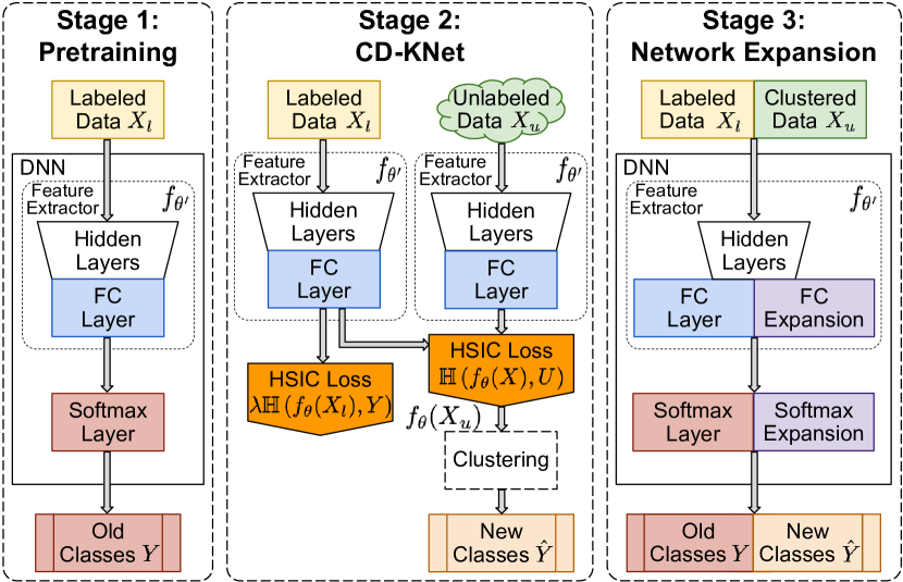
Figure 1: Overview of the CD-KNet-Exp algorithm. In Stage 1, we train a classifier (deep convolutional neural network) on labeled data $X_{l}$ from seen old classes. In Stage 2, we fine tune the feature extractor by leveraging both labeled data $X_{l}$ and unlabeled data $X_{u}$ through two HSIC-based penalties. We then cluster the unlabeled data in the learned feature embedding $f_{\theta}(X_{u})$ to generate pseudo-labels $\hat{Y}$. Finally, in Stage 3, the classifier’s penultimate (feature embedding) and last (softmax classification) layers are expanded to adjust the model to learn from both the old and new classes.

V-A An Overview of CD-KNet with Expansion

In this paper, we propose Class Discovery Kernel Network (CD-KNet) and Class Discovery Kernel Network with Expansion (CD-KNet-Exp). Our framework breaks the open-world class discovery problem into three stages, shown in Figure 1. We describe them in detail below.

During stage one, we train a deep neural network (DNN) [3] classifier from the labeled dataset $\mathcal{D}_{l}$. One can view the DNN as a combination of a non-linear feature extractor followed by a softmax classifier: the first layer until the penultimate layer of a DNN constitutes the feature extractor. Assuming the penultimate layer has $d$ dimensions (neurons), we denote this feature extractor as $f_{\theta}:\mathbb{R}^{d_{0}}\to\mathbb{R}^{d}$, parameterized by $\theta$. As usual, we refer to the output of this feature extractor $f_{\theta}(\cdot)\in\mathbb{R}^{d}$ as the latent embedding.

In stage two, we use the unsupervised data $\mathcal{D}_{u}$. Our goal is to learn from both the labeled dataset $D_{l}$ and the unlabeled data $\mathcal{D}_{u}$ for discovering the new (unseen) classes. To that end, we fine tune our feature extractor $f_{\theta}$ through our CD-KNet algorithm described in the next section. CD-KNet bridges both the supervised old classes and the unsupervised cluster (new class) discovery task through a use of two HSIC-based penalties. In addition to learning an updated latent embedding $f_{\theta}(X)$, CD-KNet also learns cluster assignments to data samples from $\mathcal{D}_{u}$. We refer to these new labels as pseudo-labels, as they abstract the newly discovered classes.

In stage three, we expand our deep network, CD-KNet-Exp, by expanding the original network with additional latent embedding nodes and output nodes to learn from both the old and new classes utilizing labels in $D_{l}$ and the pseudo-labels in $D_{u}$. This further fine-tunes both the network and our classification outcomes; it is also attuned to (and exploits) the linear separability of the latent embeddings learned by our feature extractor. Thus, whenever a new test sample comes, as long as it belongs to the $(m_{l}+m_{u})$ classes, CD-KNet-Exp can provide the prediction via the expanded neural network.

We elaborate on the details of CD-KNet and CD-KNet-Exp in the following subsections.

V-B Stage 1: Pre-training the model

As discussed above, pre-training the model involves training feature extractor $f_{\theta}:\mathbb{R}^{d_{0}}\to\mathbb{R}^{d}$, as well as a final dense/softmax layer. This can be trained over $\mathcal{D}_{l}$ via classic methods, e.g., via stochastic gradient descent (SGD) over standard loss functions (square loss, cross-entropy, etc.).

V-C Stage 2: Class Discovery Kernel Network (CD-KNet)

At the conclusion of stage one, we have learned the feature extractor $f_{\theta}$ from the DNN. In stage two, our goal is to discover new classes. A simple solution would be to leverage the learned feature extractor $f_{\theta}$ to map $D_{u}$ to the learned feature embedding space and directly perform clustering in this space (see, e.g., [10]). However, it is possible that the feature embedding space learned from the old classes in $\mathcal{D}_{l}$ are highly biased to the old classes. As a result, the learned embedding may not generalize well to $\mathcal{D}_{u}$. In our work, instead of using $f_{\theta}$ from stage one directly, we update it, forcing it to jointly adapt to both the supervised old classes in $\mathcal{D}_{l}$ as well as the unsupervised new data in $\mathcal{D}_{u}$.

Formally, following the notations in Section IV, let $X_{l}\in\mathbb{R}^{n\times d_{0}}$, $Y\in\mathbb{R}^{n\times m_{l}}$ be the data and label matrix for the labeled dataset $\mathcal{D}_{l}$ respectively, where $Y$ comprises the one-hot encoding representation of labels. Similarly, let $X_{u}\in\mathbb{R}^{n^{\prime}\times d_{0}}$ be the data matrix for the unlabeled dataset. We concatenate $X_{l}$ and $X_{u}$ to get $X\in\mathbb{R}^{(n+n^{\prime})\times d_{0}}$, a matrix containing both labeled and unlabeled datasets. We also denote by $U\in\mathbb{R}^{(n+n^{\prime})\times r}$, the corresponding latent embedding of $X$, where $r=m_{l}+m_{u}\in\mathbb{N}$ is the predefined dimensionality of the latent embedding. We learn the updated feature extractor $f_{\theta}$ and discover new classes by solving the following CD-KNet optimization problem:

$$\underset{U,\theta}{\operatorname{max}} \quad\mathbb{H}_{o}(\theta,U)=\mathbb{H}(f_{\theta}(X),U)+\lambda\mathbb{H}(f_{\theta}(X_{l}),Y),$$ (9a)

s.t. $$\quad U^{\top}U=I,$$ (9b)

where $\mathbb{H}$ is defined in Equation (3) and $\lambda\geq 0$ is the control parameter between the supervised and unsupervised objectives. We describe how to solve Prob. (9) below, in Section V-E. Intuitively, the first term encourages the separation of all classes, old and new; both should be “clusterable”, as captured by the high dependence with low-rank, orthogonal matrix $U$. The second term introduces supervised information, ensuring that the latent embedding maintains the separation between old classes, as the latter remain aligned with their labels.

As a final step of the second stage, we take $f_{\theta}(X_{u})$, the latent embedding of the new dataset, and cluster it. In more detail, upon convergence, the feature extractor $f_{\theta}$ has been refined to an extent that incorporates the information from labeled old classes as well as unlabeled new classes, resulting in a feature space which is able to separate both old and new classes well. In order to discover new classes, we feed all samples from $\mathcal{D}_{u}$ to the feature extractor to get $f_{\theta}(X_{u})$, the matrix whose rows are latent feature embedding representations of samples from $\mathcal{D}_{u}$. We then can perform any clustering method, e.g. K-means, to get the cluster assignments $\{\hat{y}_{j}\}_{j=1}^{n^{\prime}}\in\{1,\ldots,m_{u}\}^{n^{\prime}}$. Note that these $m_{u}$ clusters constitute our new classes. We refer to labels $\hat{y}_{j}$ as pseudo-labels, as they correspond to our discovered classes (that are, ideally, consistent with the ground truth classes $\mathcal{L}^{\prime}$).

The entire pipeline is illustrated in Figure 1, Stage 2. We call the pipeline as CD-KNet; the output of this stage, namely, the pseudo-labels, can be used as our final class discovery outcome. In practice, however, we further refine this with one additional stage, involving a network expansion. We describe this below. Note that, via Prob. (9), we leverage supervised information in two ways: first, via pre-training of the feature extractor, which is used as a starting point for the algorithm solving Prob. (9) below, as well as through enforcing the joint “clusterability” of both old and new latent embeddings.

V-D Stage 3: Network Expansion: CD-KNet-Exp

In our final stage, once all new samples ${X}_{u}\in\mathcal{D}_{u}$ are assigned with pseudo-labels by CD-KNet, we use these labels to retrain the network, under an appropriate network expansion [35]. We describe this in detail here. As mentioned earlier, a DNN can be regarded as the composition of a feature extractor $f_{\theta}$ and a softmax layer, i.e., the final dense layer with softmax activation. A simple heuristic to expand the network is just to expand the softmax layer by adding as many nodes as the number of new classes we have discovered. This strategy has been adopted in some prior works under a different context, such as transfer learning [36].

However, we also need to consider is the representation capacity of $f_{\theta}$. When old classes and new classes are combined, a feature extractor will naturally need more capacity, i.e. more parameters, to represent a more complex dataset. As suggested by Zeiler et al. [37], shallower layers in DNN always extract general, abstract features which are common among different tasks, while deeper layers capture specific features closely related to the task/dataset. So we decide to only expand the final layer of the feature extractor, i.e. the penultimate layer of the whole DNN, and keep the rest of the feature extractor unchanged. In practice, we find that expanding shallower layers does not affect the final performance much as overfitting may happen easily at shallower layers.

To that end, in the third stage, we expand the network by adding $m_{u}$ to the last layer, and 25% to the penultimate layer. The expanded model is then fine-tuned over both $\mathcal{D}_{l}$ and $\mathcal{D}_{u}$. In particular, the model is fine-tuned on $\mathcal{D}_{u}$ with pseudo-labels $\hat{Y}_{u}$ to incorporate new classes. In addition to learning from $\mathcal{D}_{u}$ and the new classes, we also include a fraction $p\%$ of the old classes $\mathcal{D}_{l}$ to strengthen previous learned knowledge from seen old classes. We refer to this as fine-tuning rather than training, because we lower the learning rate of the expanded model, except its expanded two final layers. It is also possible to just retrain a new model, however, in our experiments, we find that fine-tuning the model always converges better and faster than retraining a model from scratch. Overall, the process of network expansion is summarized and presented in Stage 3 in Figure 1. We refer to the complete 3-stage pipeline as CD-KNet-Exp. The final outputs of this process are the labels produced by the expanded model over $\mathcal{D}_{u}$.

V-E Solving the CD-KNet Optimization Problem

We adopt an alternating optimization strategy to learn $\theta$ and $U$ iteratively. The whole process is shown in Algorithm 1.

Input: whole dataset matrix $X$, labeled dataset matrix $X_{l}$ and its corresponding label matrix $Y\in\mathbb{R}^{n\times m_{l}}$

Output: parameter of feature extractor $\theta$, cluster assignments of $\mathcal{D}_{u}$

Initialization: initialize $\theta$ by training on $\mathcal{D}_{l}$;

initialize $U$ by spectral embedding of $f_{\theta}(X)$

while $\theta$ has not converged do

       Update $\theta$ via one epoch of SGD via Eq. (10) and (11) alternatingly, while keeping $U$ fixed.

       Update $U$ via eigendecomposition according to Eq. (14).

end while

Cluster $f_{\theta}(X_{u})$ to get cluster assignments.

Algorithm 1 CD-KNet Algorithm

Initialization: $\theta$ is initialized by the supervised training in stage one. We initialize $U$ by conducting spectral clustering on $f_{\theta}(X)$, which is equivalent to (7) [31].

Updating $\theta$: Assuming $U$ is fixed, we update $\theta$ via gradient ascent. In practice, we would like to update $\theta$ using stochastic gradient ascent via mini-batches. However, if we randomly sample mini-batches among all samples, we need to keep track of labeled and unlabeled parts inside each mini-batch. Thus, we simplify the process by optimizing the supervised and unsupervised part of $\mathbb{H}_{o}$ iteratively. First, we sample an unlabeled mini-batch $X_{b}$ from $X$, updating $\theta$ by:

$$\theta:=\theta+\gamma\nabla\mathbb{H}(f_{\theta}(X_{b}),U_{b}),$$ (10)

where $\gamma$ is the learning rate and $U_{b}$ is the corresponding latent cluster embedding for this mini-batch. Then, we sample a mini-batch $X_{b}$ from $X_{l}$, updating $\theta$ by:

$$\theta:=\theta+\lambda\gamma\nabla\mathbb{H}(f_{\theta}(X_{b}),Y_{b}),$$ (11)

where the learning rate $\gamma$ remains the same as in the previous step and $Y_{b}$ is the corresponding label matrix for this mini-batch. We update $\theta$ for an epoch before we update $U$.

Updating $U$: When $\theta$ is fixed, the optimization in Equation (9) w.r.t $U$ alone is equivalent to:

$$\underset{U}{\operatorname{max}} \quad\text{tr}(U^{\top}HD^{-1/2}K_{f_{\theta}(X)}D^{-1/2}HU),$$ (12)

s.t. $$\quad U^{\top}U=I,$$ (13)

where here we used $K_{U}=UU^{\top}$, $\text{tr}(\cdot)$ to represent the trace of a matrix and applied the cyclic property of the trace. This maximization problem of $U$ can be solved via eigendecomposition. The optimal solution for $U$ is given by the top $r$ eigenvectors of the following matrix:

$$\mathcal{L}_{\theta}=HD^{-1/2}K_{f_{\theta}(X)}D^{-1/2}H,$$ (14)

where $H$ is as in Eq. (3), and $D$ is the degree matrix given by Eq. (6).

Subsampling: While the number of labeled and unlabeled samples $n$, $n^{\prime}$ could be very large, it is often time and resource consuming to compute $\mathbb{H}_{o}$ using all of the data. As an alternative, we perform subsampling to compute and optimize $\mathbb{H}_{o}$. Specifically, we sample $n_{1}$ labeled samples from $\mathcal{D}_{l}$ and $n^{\prime}_{1}$ unlabeled samples from $\mathcal{D}_{u}$, where $n_{1}\ll n$ and $n^{\prime}_{1}\ll n^{\prime}$. We then form labeled data matrices $X_{l1}\in\mathbb{R}^{n_{1}\times d_{0}}$ as well as its corresponding label matrix $Y_{1}\in\mathbb{R}^{n_{1}\times m_{l}}$, and unlabeled data matrix $X_{u1}\in\mathbb{R}^{n^{\prime}_{1}\times d_{0}}$. We concatenate $X_{l1}$ and $X_{u1}$ to get $X_{1}\in\mathbb{R}^{(n_{1}+n^{\prime}_{1})\times d_{0}}$ and define latent embedding $U_{1}\in\mathbb{R}^{(n_{1}+n^{\prime}_{1})\times r}$. Finally, we replace $X,U,X_{l},Y$ with $X_{1},U_{1},X_{l1},Y_{1}$ in Equation (9) and solve the corresponding optimization problem. Our experiments show that using only 5% of the original dataset suffices to get a good performance.

VI Experiments

In this section, we investigate how our proposed method CD-KNet-Exp compares against competing methods on three benchmark datasets and one real world radio frequency fingerprinting dataset. We also conduct comprehensive experiments to explore the effects of different controllable parameters on the performance of our algorithm.

VI-A Datasets

Our proposed Class Discovery Kernel Network with Expansion (CD-KNet-Exp) method is evaluated on three benchmark datasets, MNIST, Fashion MNIST and CIFAR-100, as well as a real world dataset of radio frequency transmissions (RF-50).

MNIST. MNIST is a well-known database of grayscale images of handwritten decimal digits [38]. The dataset contains $60,000$ digits in the training set, and $10,000$ digits in the test set. In our experiments, we select the first 5 digits as the labeled, old classes, while the rest last 5 digits to constitute a set of unlabeled, new classes.

Fashion MNIST. Fashion MNIST was first introduced by Xiao et al. in [39], and contains grayscale images of 10 types of fashion products, including clothes, shoes, and accessories. Fashion MNIST follows the original MNIST dataset in image size and structure of training and test splits; however, each class is represented by exactly $7,000$ images. Again, a set of labeled classes consists of the first 5 fashion products, while the rest 5 classes are treated as unlabeled.

CIFAR-100. CIFAR-100 is another imaging dataset that contains $60,000$ color images of 100 categories of objects, with $6,000$ images per category. Here, the dataset comprises of $50,000$ training and $10,000$ testing images. In analogy to MNIST datasets, object categories in CIFAR-100 are split into labeled and unlabeled, with the first 70 classes belonging to the former group and 30 included in the latter one.

RF-50. This dataset contains $8,800$ radio transmissions from $50$ WiFi devices recorded in the wild [40, 41]. Wireless signals undergo equalization [41]. The dataset is split as follows: $141$ recordings from each device constitute the training subset, while $35$ are used for testing. Also, we randomly choose $35$ devices and mark them as labeled, i.e. they form $\mathcal{D}_{l}$ part of data, and the other $15$ devices are considered as unlabeled, i.e. form the $\mathcal{D}_{u}$ dataset.

VI-B Competing Methods

As mentioned in the related work section, open-world class discovery is a relatively new problem that is insufficiently investigated at the moment, and only one direct competitor with reproducible code is available [10]. Nevertheless, we devise simple baselines via variations of our own framework. We also compare against state-of-the-art deep clustering methods to strengthen our empirical results.

Our variants:
CD-KNet-Exp. CD-KNet-Exp is our proposed class discovery kernel network approach as described in Section VI-B and summarized in Figure 1. Next, we perform an ablation study and describe three modifications of our framework designed to understand the importance of each core component.
CD-KNet. To understand the importance of network expansion to accurately predict new classes $\hat{Y}$, we compare against CD-KNet which is a variant of our approach without the expansion (i.e., it only completes the first two stages of the framework).
UCD-KNet-Exp. Another crucial component of the proposed method is the incorporation of both supervised old class data and the unlabeled data in learning our feature extractor $f_{\theta}$ based on Objective 9a. To evaluate the influence of supervision, we set $\lambda=0$ in Eq. 9a, and treat this unsupervised variant, UCD-KNet-Exp, as another competitor.
UCD-KNet. Finally, we remove both network expansion and supervised components of the proposed CD-KNet-Exp framework, and consider this simplest unsupervised variant as UCD-KNet.

We compare against the current state-of-the-art approach to class discovery, Semi-Supervised Class Discovery (SSCD) [10].
SSCD. Nixon et al. [10] propose a framework for a new class discovery based on the idea of (a) training a classifier on known classes, (b) applying it to unseen classes, (c) detecting new classes via K-means clustering, and (d) expanding the classifier via pseudo-labels. This is can be seen as a simple “clustering plus supervised learning” baseline compared to CD-KNet-Exp, skipping the additional retraining via HSIC. Originally, the SSCD framework adopts the work of Hendrycs and Gimpel [42] to detect ‘new class’-candidate data samples. However, because novelty detection is not the focus of this paper, and in order to perform a fair comparison with our method, we assume that all test samples do not belong to the known classes, eschewing the novelty detection component.
SSCD-Exp. For their method, Nixon and others propose to expand a classification model solely in the last layer to accommodate the increased number of classes, and then retrain the model on data with both original and clustered labels. Here, we adapt/modify the original SSCD method with our proposed strategy to expand their classification model. As in the 3rd stage of our method, we expand their neural network both in the penultimate and ultimate layers. Hereinafter, we refer to this method as SSCD-Exp. Both SSCD and SSCD-Exp are implemented in accordance with the description and parameter settings provided in the original paper. We did not compare to Shu et al. [9], as no code is publicly available; we note however that the NMI they report on MNIST is 0.48, far lower than CD-KNet-Exp (0.856) and other competitors.

Finally, we also compare against two state-of-the-art deep learning-based clustering algorithms.
Deep Embedding Clustering (DEC). In [43], the authors use stacked autoencoder to map the input $X_{u}$ to the low-dimensional feature space and then perform K-means clustering to initialize $m_{u}$ cluster centroids. The main idea behind DEC is to obtain probabilistic cluster assignments and then iteratively update them using the Kullback-Leibler divergence between the distribution of such “soft” assignment values and some auxiliary distribution.
Deep Adaptive Clustering (DAC). DAC [44] re-casts a clustering task to a binary pair-wise classification problem. DAC is an iterative method for assigning a pair of inputs to the same class if their embeddings are similar enough, assign to different classes if embeddings are different enough; otherwise, it discards the pair from the current training iteration. The similarity and dissimilarity thresholds in DAC are changed adaptively after each iteration. In the experiments, we utilize the original implementations provided by the authors for both DEC and DAC methods.

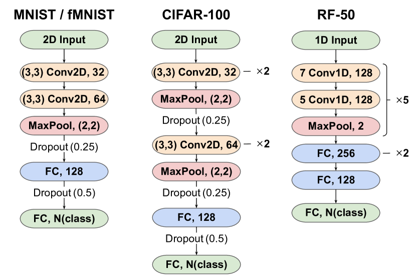
Figure 2: Network architectures used for MNIST/fashion MNIST, CIFAR-100, and RF-50 datasets.

VI-C Implementation Details

For both MNIST, Fashion MNIST, and CIFAR-100 datasets, we employ convolutional neural networks suggested in the official Keras Examples Directory for the corresponding datasets [45]. For the RF-50 dataset, we applied the baseline convolutional neural network proposed in [40]. All three models are illustrated on Figure 2.

TABLE II: Number of epochs for each dataset at different stages. We use the same numbers for MNIST and Fashion-MNIST.

Dataset	Pretraining	CD-KNet	Network Expansion
(Fashion) MNIST	50	20	30
CIFAR-100	70	20	30
RF-50	25	10	25

We determined all the hyperparameters on a validation set via holding out $10\%$ of the training data. For all experiments, we use the same learning rates for Stages one and two. For Stage three, the network expansion stage, we use the same learning rate again to train the expanded last two layers and $0.1$ of the learning rate to fine tune the rest of the network. The proportion of $\mathcal{D}_{l}$ samples used in training network expansion is $20\%$. For MNIST and Fashion-MNIST, we use Adam [46] optimizer with a learning rate of $0.01$. For CIFAR-100, we use Adam optimizer with a learning rate of $0.0001$. For RF-50, we followed the suggested hyperparameters by Jian et al. [40]. The training epochs for Stage one (pretraining), Stage two (CD-KNet), and Stage three (network expansion) are summarized in Table II. We set $\lambda=10$ and the subsampling rates for MNIST, Fashion-MNIST, CIFAR-100 and RF-50 as $3\%$, $5\%$, $5\%$, $5\%$, respectively. We implement our method using Keras 2.2.4 [47] and TensorFlow 1.14.0 [48]. Our source code is publicly available.

VI-D Evaluation Metrics

We assess the quality of the clusters discovered by our proposed class discovery approach, CD-KNet-Exp, and the other competing methods described in Section VI-B on the unlabeled data $D_{u}$ using clustering evaluation metrics. In particular, we report the following three clustering external evaluation metrics: clustering accuracy (ACC), normalized mutual information (NMI) and adjusted Rand index (ARI). These external evaluation criteria measure how well the discovered clusters match the ground truth unseen class labels. ACC is the standard clustering accuracy measure. NMI is the normalized mutual information between the estimated cluster pseudo-labels $\hat{y}_{u}$ and the ground-truth labels $y_{u}$: $\mathtt{NMI}(\hat{y}_{u},y_{u})=\frac{I(\hat{y}_{u},y_{u})}{\sqrt{H(\hat{y}_{u})H(y_{u})}}$, where $I(a,b)$ is the mutual information between $a$ and $b$, and $H(a)$ and $H(b)$ are the entropies of $a$ and $b$ respectively. Both $I$ and $H$ here are computed from empirical distributions. Finally, ARI is the adjusted Rand index, which measures the amount of overlap between two clustering solutions as follows:

$$\mathtt{ARI}=\frac{\mathtt{RI}-E[\mathtt{RI}]}{\max(\mathtt{RI})-E[\mathtt{RI}]},\text{ where }\mathtt{RI}=\frac{a+b}{C^{n}_{2}},\text{ and}$$ (15)

where $a$ is the number of pairs of data samples that belong to the same class w.r.t. both the ground-truth and pseudo-labels, $b$ is the number of data samples that belong to the different classes w.r.t. both the ground-truth and pseudo-labels, and $C^{n}_{2}$ is the total number of data sample pairs in the dataset. All three metrics have values between zero and one. The higher the value, the better the clustering agreement with the true labels.

VII Results and Discussion

VII-A Results on Benchmark Datasets and Radio Dataset

TABLE III: Class discovery performance on all datasets.

Datasets	MNIST			Fashion-MNIST			CIFAR-100			RF-50
Methods\Metrics	ACC	NMI	ARI	ACC	NMI	ARI	ACC	NMI	ARI	ACC	NMI	ARI
SSCD	0.840	0.629	0.649	0.552	0.386	0.316	0.201	0.193	0.064	0.524	0.194	0.184
SSCD-Exp	0.887	0.791	0.812	0.596	0.477	0.376	0.213	0.204	0.066	0.578	0.230	0.220
UCD-KNet	0.849	0.645	0.664	0.587	0.476	0.403	0.220	0.216	0.078	0.553	0.244	0.273
UCD-KNet-Exp	0.926	0.794	0.829	0.622	0.518	0.470	0.247	0.237	0.091	0.585	0.279	0.309
CD-KNet	0.869	0.683	0.707	0.655	0.535	0.463	0.232	0.228	0.080	0.587	0.453	0.456
CD-KNet-Exp	0.945	0.856	0.869	0.679	0.603	0.529	0.269	0.256	0.102	0.610	0.481	0.485

Class Discovery Performance. In Table III we report the class discovery performance, in terms of ACC, NMI and ARI, of our proposed CD-KNet-Exp method, along with all other competing methods on all datasets. Note that in all datasets, CD-KNet-Exp performs the best against all methods w.r.t. all three clustering metrics.

From this table, we can also observe the effect of network expansion compared to versions without (‘Exp’). Note that all the methods which incorporate network expansion gain performance increase over their counterpart, showing the effectiveness of this strategy.

Another interesting observation from Table III is that our CD-KNet-Exp and UCD-KNet-Exp achieve the 1st and 2nd best performance consistently on all datasets. This demonstrates that (a) only using the unsupervised part in our HSIC objective already leads to better separable latent feature embeddings than other methods; and (b) introducing supervised knowledge from old classes further improves the performance of only using unsupervised information.

TABLE IV: Comparing with full unsupervised learning methods.

Datasets	MNIST			Fashion-MNIST			CIFAR-100
Methods\Metrics	ACC	NMI	ARI	ACC	NMI	ARI	ACC	NMI	ARI
DEC	0.873	0.835	0.822	0.620	0.566	0.522	0.205	0.166	0.073
DAC	0.894	0.843	0.865	0.642	0.588	0.543	0.247	0.195	0.088
CD-KNet-Exp	0.945	0.856	0.869	0.679	0.603	0.529	0.269	0.256	0.102

Comparing with Unsupervised Deep Learning Methods. In order to show that our method provides an effective way of incorporating knowledge learned from old classes, we compare our method with two state-of-the-art deep learning based unsupervised clustering methods, DEC [43] and DAC [44], on three benchmark datasets in Table IV. To mimic our problem setting, we pretrain the deep neural networks used in DEC and DAC with old classes, and then we perform these algorithms on new classes. Table IV shows that CD-KNet-Exp beats both of the methods on all three benchmarks. Although we enforce DEC and DAC to incorporate knowledge from old classes by pretraining, our method still outperforms both DEC and DAC.

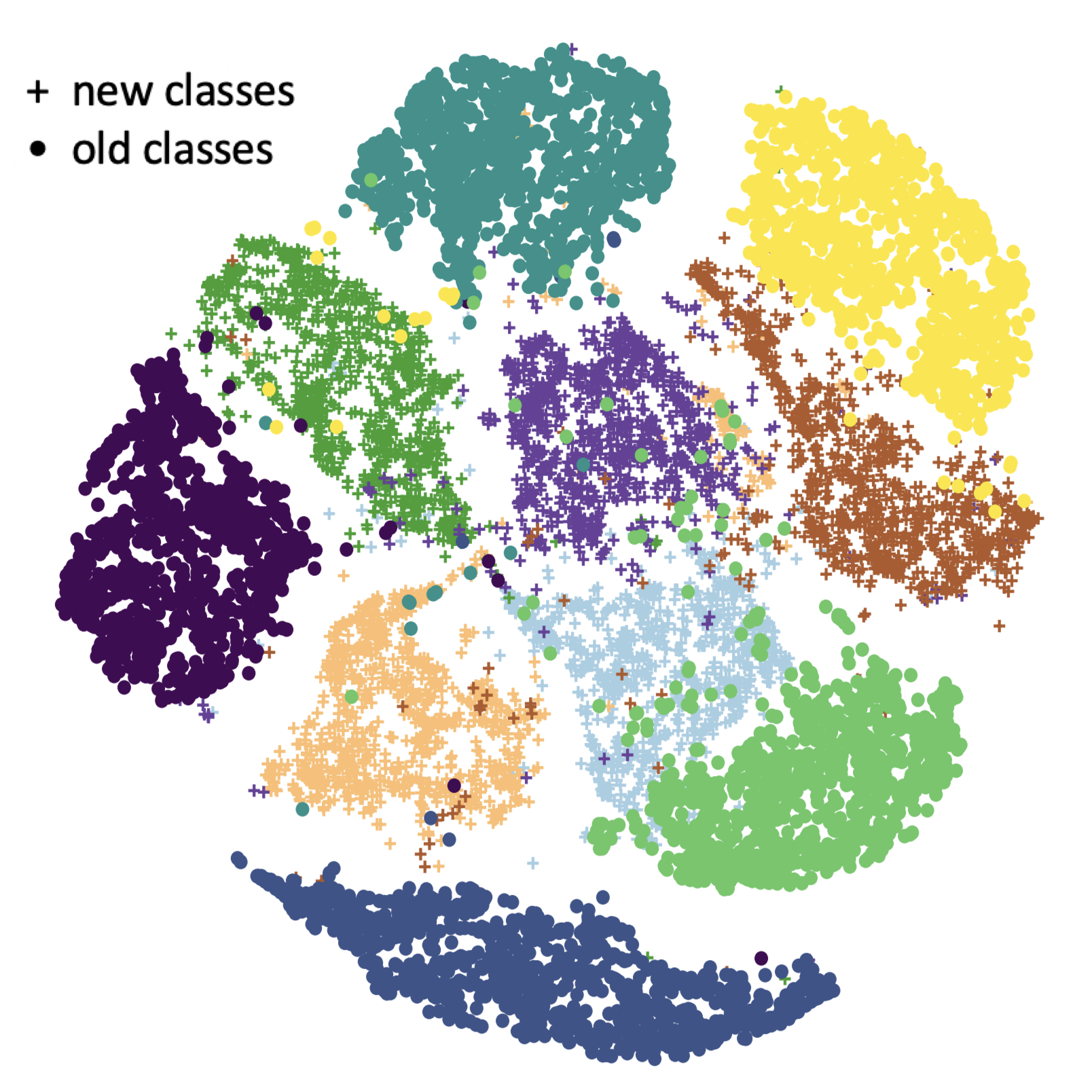
(a) CD-KNet-Exp

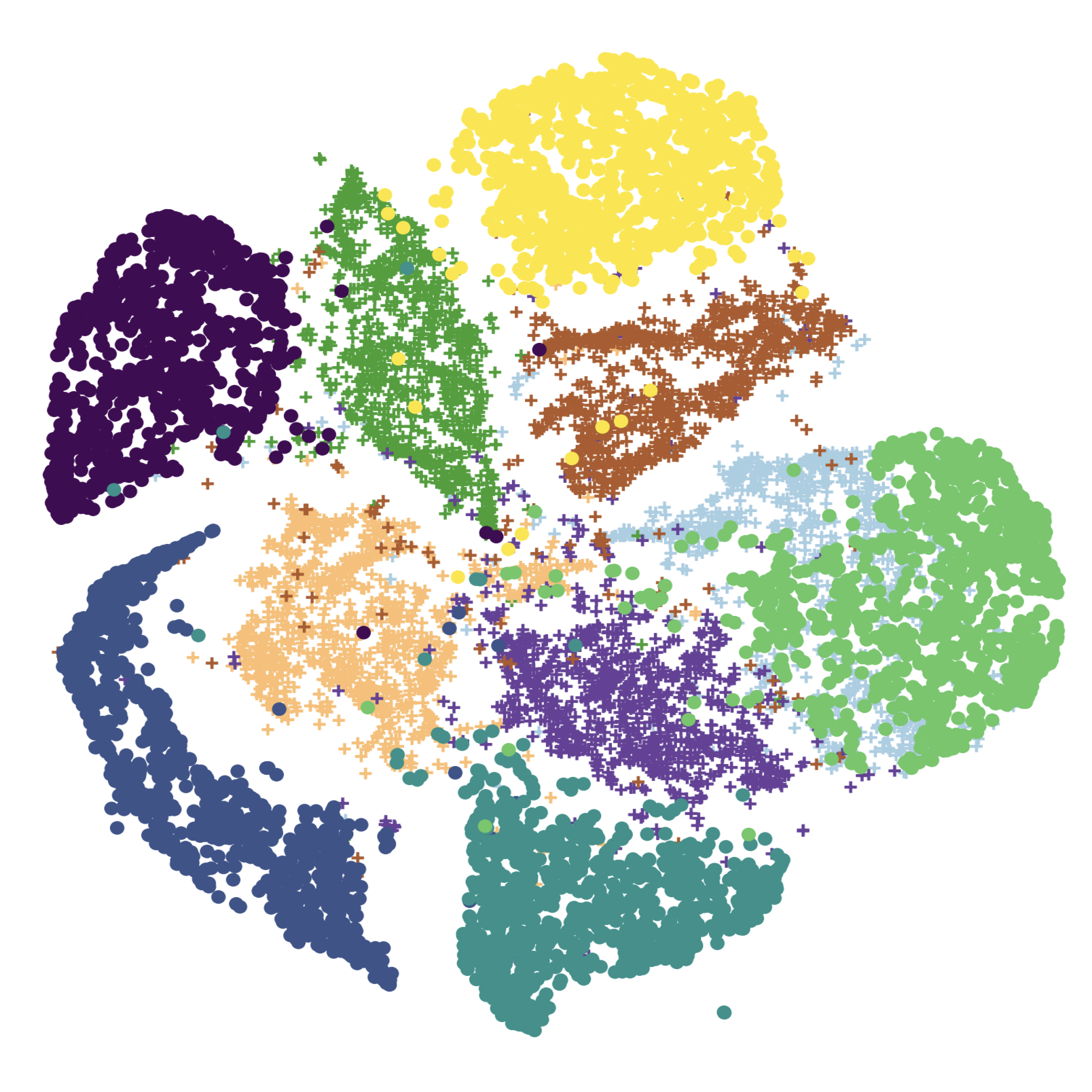
(b) SSCD-Exp

Figure 3: t-SNE visualization of latent embeddings of CD-KNet-Exp and SSCD-Exp. CD-KNet-Exp 1) produces better separable latent embeddings than SSCD-Exp; 2) has clearer boundaries between old and new classes.

Visualization of Latent Embeddings. In Figure 3, we investigate the latent embeddings learned by our method CD-KNet-Exp against the state-of-the-art method for class discovery SSCD-Exp on the MNIST dataset. We plot the embeddings using t-SNE [49] visualization of the latent feature embedding after expansion for all classes, where ‘$+$’ represents new classes, ‘$\bullet$’ represents old classes, and different colors represent different classes. Observe that CD-KNet-Exp separates the classes better than SSCD-Exp. Also, we notice that SSCD mixes one of the new classes (light blue) and old classes (green) together. This explains why there is an accuracy drop on the old classes (which we will explain later in Table VI). Recall that SSCD directly uses feature extractor learned on old classes, so that it has an underlying drawback of mistaking new classes to old ones when their samples are similar in the latent embedding space. In contrast, CD-KNet-Exp takes both labeled old classes and unlabeled new classes into consideration, pulling them apart in the learned latent embedding space by optimizing the CD-KNet HSIC based objective.

VII-B Influence of Controllable Parameters.

Our method, CD-KNet-Exp has several controllable parameters: the control parameter $\lambda$ between supervised and unsupervised HSIC, network expansion, and the subsampling factor. In this subsection, explore how these parameters affect the final class discovery performance.

TABLE V: Influence of $\lambda$ on Fashion MNIST dataset.

Metric\$\lambda$	10	0	$\infty$
ACC	0.655	0.587	0.544
NMI	0.535	0.476	0.375
ARI	0.463	0.403	0.276

Influence of $\lambda$. In Equation (9a), we have a balance factor $\lambda$ to control how much weight to put on the supervised part of our HSIC based objective. In practice, we find that the algorithm is not sensitive to the value of $\lambda$ for a wide range ($\lambda\in[1,100]$) of values, so we just set $\lambda=10$ as a representative value in our experiments. However, we observe clear differences in performance when there is only unsupervised information ($\lambda=0$), supervised and unsupervised information ($\lambda=10$) and only supervised information ($\lambda=\infty$, in practice, we enforce this by removing the unsupervised term).

Table V reports the class discovery performance in terms of ACC, NMI and ARI of CD-KNet-Exp for $\lambda=10$, $\lambda=0$, and $\lambda=\infty$ on Fashion-MNIST dataset. When Comparing $\lambda=10$ and $\lambda=0$, we are actually comparing CD-KNet-Exp and UCD-KNet-Exp. The better performance of CD-KNet-Exp over unsupervised UCD-KNet-Exp showcases the importance of supervision in our HSIC based objective, which is also demonstrated in Table III. Interestingly, $\lambda=\infty$ results in the worst performance, indicating that only using supervised HSIC to tune the network tends to overfit to old classes, resulting in poor performance on the new classes.

Influence of Network Expansion. We have already shown how network expansion helps new class discovery in Table III. In this subsection, we investigate the effect of expansion on the classification accuracy on the previous old classes. Table VI shows the cluster accuracy and classification accuracy of new and old classes respectively, before expansion and after expansion on the MNIST dataset. Both CD-KNet-Exp and UCD-KNet-Exp incorporate network expansion strategy well with clustering accuracy increase on new classes and almost no classification accuracy decrease on old classes. In contrast, although SSCD achieves better cluster accuracy on new classes after expansion, the classification accuracy of SSCD on old classes drops by about $10\%$.

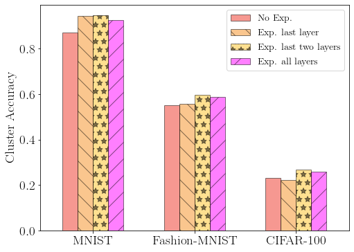
Figure 4: Comparison of different expansion strategies and no expansion. Expansion of the last two layers of the network performs the best among all strategies.

Comparing Different Expansion Strategies. To justify the reason why we choose to expand the last two layers of the DNN, we compare 3 different expansion strategies and completely no expansion. The 3 expansion strategies are: (a) Expand only the last layer; (b) Expand the last two layers (ours); and, (c) Expand all layers in the DNN (for convolutional layers, we double its number of filters). Figure 4 demonstrates that our strategy, expanding the last two layers, indeed performs the best. Moreover, note that an all expansion strategy performs better than no expansion. On MNIST dataset, expanding only the last layer is comparable with our strategy. However, on Fashion-MNIST and CIFAR-100, there is a performance gap between expanding only the last layer and the last two layers. This observation suggests that the feature extractor has enough representation capacity for relatively simple datasets like MNIST, but for complex datasets, we need to expand the feature extractor to allocate more representation power for new classes. On the other hand, expanding all layers which increases the representation capacity of the DNN leads to worse performance than just expanding the last two layers. This is a case of overfitting, which may harm the performance when we expand the DNN too much.

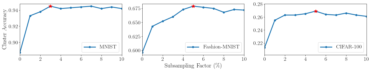
Figure 5: Influence of subsampling factor w.r.t. $\mathtt{ACC}$ measure. CD-KNet-Exp is able to perform well using only 3%, 5%, 5% of the MNIST, Fashion-MNIST and CIFAR-100 datasets, respectively.

Influence of Subsampling Factor. As mentioned in Section V-E, calculating the kernel matrix for all the data is computationally expensive, so we adopt a subsampling strategy [33] to reduce the computation. In Fig 5, we explore how the subsampling factor will affect the final performance. For each benchmark dataset, we set the subsampling factor from $0\%$ (equivalent to SSCD) to $10\%$. The trends are very similar for all datasets: There is a notable jump in accuracy from $0\%$ to $1\%$ and then the accuracy increase slows down until it reaches the best performance ($3\%$ for MNIST and $5\%$ for Fashion-MNIST and CIFAR-100). After that, the accuracy tends to be stable. These empirical results show that CD-KNet only needs a small portion of the data to capture the whole picture, generalizing well to the entire dataset.

TABLE VI: Influence of Network Expansion on MNIST dataset w.r.t. $\mathtt{ACC}$ measure

	New Classes		Old Classes
Method\Stage	Before	After	Before	After
SSCD-Exp	0.840	0.887	0.988	0.892
U-KNet-Exp	0.849	0.926	0.988	0.983
CD-KNet-Exp	0.869	0.945	0.988	0.983

VIII Conclusions

In this paper, we introduced CD-KNet-Exp for addressing the open-world class discovery problem. Empirical results on MNIST, Fashion-MNIST, CIFAR-100 and a real-world radio frequency fingerprinting dataset, RF-50, show that CD-KNet-Exp can discover new classes with clustering performance better than all competing methods. In particular, it outperforms competitors over three benchmark datasets by a $2\%$-$12\%$ margin.

IX Acknowledgements

The authors gratefully acknowledge support by the National Science Foundation (grant CCF-1937500).

References

- [1] A. Bendale and T. Boult, “Towards open world recognition,” in CVPR, 2015, pp. 1893–1902.
- [2] W. J. Scheirer et al., “Toward open set recognition,” TPAMI, vol. 35, no. 7, pp. 1757–1772, 2012.
- [3] Y. LeCun, Y. Bengio, and G. Hinton, “Deep learning,” nature, vol. 521, no. 7553, pp. 436–444, 2015.
- [4] K. He et al., “Deep residual learning for image recognition,” in CVPR, 2016, pp. 770–778.
- [5] A. Krizhevsky et al., “Imagenet classification with deep convolutional neural networks,” in NerIPS, 2012, pp. 1097–1105.
- [6] J. Devlin et al., “BERT: pre-training of deep bidirectional transformers for language understanding,” in NAACL-HLT, 2019, pp. 4171–4186.
- [7] A. Bendale and T. E. Boult, “Towards open set deep networks,” in CVPR, 2016, pp. 1563–1572.
- [8] G. Fei and B. Liu, “Breaking the closed world assumption in text classification,” in NAACL-HLT, 2016, pp. 506–514.
- [9] L. Shu, H. Xu, and B. Liu, “Unseen class discovery in open-world classification,” arXiv preprint arXiv:1801.05609, 2018.
- [10] J. Nixon, J. Liu, and D. Berthelot, “Semi-supervised class discovery,” arXiv preprint arXiv:2002.03480, 2020.
- [11] M. A. Pimentel, D. A. Clifton, L. Clifton, and L. Tarassenko, “A review of novelty detection,” Signal Processing, vol. 99, pp. 215–249, 2014.
- [12] Z. Chen and B. Liu, “Lifelong machine learning,” Synthesis Lectures on Artificial Intelligence and Machine Learning, vol. 10, pp. 1–145, 2016.
- [13] S. Subramaniam et al., “Online outlier detection in sensor data using non-parametric models,” in VLDB, 2006, pp. 187–198.
- [14] Y. Bengio, H. Larochelle, and P. Vincent, “Non-local manifold parzen windows,” in NerIPS, 2006, pp. 115–122.
- [15] F. Angiulli and C. Pizzuti, “Fast outlier detection in high dimensional spaces,” in PKDD, 2002, pp. 15–27.
- [16] V. Hautamaki, I. Karkkainen, and P. Franti, “Outlier detection using k-nearest neighbour graph,” in ICPR, vol. 3, 2004, pp. 430–433.
- [17] J. Zhang et al., “Detecting outlying subspaces for high-dimensional data: the new task, algorithms, and performance,” KAIS, vol. 10, 2006.
- [18] R. Chalapathy, A. K. Menon, and S. Chawla, “Anomaly detection using one-class neural networks,” arXiv preprint arXiv:1802.06360, 2018.
- [19] A. Gritsenko, Z. Wang, T. Jian et al., “Finding a ‘new’needle in the haystack: Unseen radio detection in large populations using deep learning,” in DySPAN, 2019, pp. 1–10.
- [20] N. Grira, M. Crucianu, and N. Boujemaa, “Unsupervised and semi-supervised clustering: a brief survey,” A review of machine learning techniques for processing multimedia content, vol. 1, pp. 9–16, 2004.
- [21] X. Zhu and A. B. Goldberg, “Introduction to semi-supervised learning,” Synthesis lectures on artificial intelligence and machine learning, 2009.
- [22] T. N. Kipf and M. Welling, “Semi-supervised classification with graph convolutional networks,” in ICLR, 2017.
- [23] A. Rasmus et al., “Semi-supervised learning with ladder networks,” in NerIPS, 2015, pp. 3546–3554.
- [24] X. Yin et al., “Semi-supervised clustering with metric learning: An adaptive kernel method,” Pattern Recognition, vol. 43, no. 4, 2010.
- [25] S. Basu, M. Bilenko, and R. J. Mooney, “A probabilistic framework for semi-supervised clustering,” in SIGKDD, 2004, pp. 59–68.
- [26] S. Lloyd, “Least squares quantization in pcm,” IEEE transactions on information theory, vol. 28, no. 2, pp. 129–137, 1982.
- [27] M. Markou and S. Singh, “Novelty detection: a review,” Signal processing, vol. 83, no. 12, pp. 2481–2497, 2003.
- [28] E. Lughofer, “A dynamic split-and-merge approach for evolving cluster models,” Evolving Systems, vol. 3, no. 3, pp. 135–151, 2012.
- [29] A. Gretton et al., “Measuring statistical dependence with hilbert-schmidt norms,” in ALT, 2005, pp. 63–77.
- [30] L. Song et al., “Feature selection via dependence maximization,” Journal of Machine Learning Research, vol. 13, pp. 1393–1434, 2012.
- [31] D. Niu, J. Dy, and M. I. Jordan, “Dimensionality reduction for spectral clustering,” in AISTATS, 2011, pp. 552–560.
- [32] C. Wu, S. Ioannidis, M. Sznaier et al., “Iterative spectral method for alternative clustering,” in AISTATS, 2018, pp. 115–123.
- [33] C. Wu, Z. Khan, S. Ioannidis, and J. G. Dy, “Deep kernel learning for clustering,” in ICDM. SIAM, 2020, pp. 640–648.
- [34] C. Wu et al., “Solving interpretable kernel dimensionality reduction,” in Advances in NeurIPS, 2019, pp. 7913–7923.
- [35] D. Marnerides et al., “Expandnet: A deep convolutional neural network for high dynamic range expansion from low dynamic range content,” in Computer Graphics Forum, vol. 37, no. 2, 2018, pp. 37–49.
- [36] C. Tan et al., “A survey on deep transfer learning,” in International conference on artificial neural networks. Springer, 2018, pp. 270–279.
- [37] M. D. Zeiler and R. Fergus, “Visualizing and understanding convolutional networks,” in ECCV, 2014, pp. 818–833.
- [38] Y. LeCun et al., “Gradient-based learning applied to document recognition,” Proceedings of the IEEE, vol. 86, no. 11, pp. 2278–2324, 1998.
- [39] H. Xiao et al., “Fashion-mnist: a novel image dataset for benchmarking machine learning algorithms,” arXiv preprint arXiv:1708.07747, 2017.
- [40] T. Jian et al., “Deep learning for rf fingerprinting: A massive experimental study,” IEEE Internet of Things Mag., vol. 3, pp. 50–57, 2020.
- [41] S. Riyaz et al., “Deep learning convolutional neural networks for radio identification,” IEEE Communications Mag., vol. 56, pp. 146–152, 2018.
- [42] D. Hendrycks and K. Gimpel, “A baseline for detecting misclassified and out-of-distribution examples in neural networks,” in ICLR, 2017.
- [43] J. Xie, R. Girshick, and A. Farhadi, “Unsupervised deep embedding for clustering analysis,” in ICML, 2016, pp. 478–487.
- [44] J. Chang et al., “Deep adaptive image clustering,” in ICCV, 2017, pp. 5879–5887.
- [45] “Keras Examples Directory,” https://github.com/keras-team/keras/tree/master/examples, accessed: 2020-09-21.
- [46] D. P. Kingma and J. Ba, “Adam: A method for stochastic optimization,” in ICLR, 2015.
- [47] F. Chollet et al., “Keras,” https://github.com/fchollet/keras, 2015.
- [48] M. Abadi et al., “TensorFlow: Large-scale machine learning on heterogeneous systems,” 2015.
- [49] L. V. D. Maaten and G. Hinton, “Visualizing data using t-sne,” Journal of machine learning research, vol. 9, no. Nov, pp. 2579–2605, 2008.