Highly Accurate Closed-form Approximation for the
Probability of Detection of Weibull Fluctuating Targets in Non-Coherent Detectors

Abstract

In this paper, we derive a highly accurate approximation for the probability of detection (PD) of a non-coherent detector operating with Weibull fluctuation targets. To do so, we assume a pulse–to–pulse decorrelation during the coherent processing interval (CPI). Specifically, the proposed approximation is given in terms of: i) a closed-form expression derived in terms of the Fox’s $H$-function, for which we also provide a portable and efficient MATHEMATICA routine; and ii) a fast converging series obtained through a comprehensive calculus of residues. Both solutions are fast and provide very accurate results. In particular, our series representation, besides being a more tractable solution, also exhibits impressive savings in computational load and computation time compared to previous studies. Numerical results and Monte-Carlo simulations corroborated the validity of our expressions.

I Introduction

The target’s radar cross section (RCS) plays an important role in radar detection. Specifically, RCS is a measure that describes the amount of energy reflected by a target and, therefore, has a direct impact on the received target echo power. In general, RCS is a complex function of: target geometry and material composition; position of transmitter relative to target; position of receiver relative to target; frequency or wavelength; transmitter polarization; and receiver polarization [1]. Since the target’s RCS is extremely sensitive to the above parameters, it is common and more practical to use statistical models to capture its behavior [2]. This argument leads to consider the target’s RCS as a random variable (RV) with a specified probability density function (PDF). It is important to emphasize that using statistical models for the RCS does not imply that the actual RCS is random. If it was possible to describe the target surface shape, materials and location in enough detail, then the target’s RCS could in principle be calculated accurately using deterministic approaches [3]. However, in practice, this task seems to be extremely complicated and too demanding to be executed.

Some common statistical models for the target’s RCS are the Exponential and the fourth-degree Chi-square distributions. Both distributions are part of the well-known Swerling models, also known as fluctuating target models [4]. The Exponential distribution arises when there is a large number of individual scatterers randomly distributed in space and each with approximately the same individual RCS. The Exponential distribution is used in the Sweling cases I and II [4, 5, 6]. For the case when there is a large number of individual scatterers, one dominant and the rest with the same RCS, the Exponential distribution is no longer a good fit for the target’s RCS. The noncentral Chi-square distribution with two degrees of freedom is the exact PDF for this case, but it is considered somewhat difficult to work with because the expression for the PDF contains a Bessel function. For this reason, the fourth-degree Chi-square distribution is used in the Swerling cases III and IV since it is a more analytically tractable approximation [6, 7, 8].

More robust target models emerge so as to accurately describe the complex behaviour of the target’s RCS. Among them, we highlight the Log-normal, Chi-square and Weibull target models. These models are widely used in high-resolution radars, in which the resolution cell is small enough to contain a reduced number of scatterers [9, 10, 11, 12]. In particular, the Log-normal and Weibull target models provide an excellent empirical fit to observed data since they exhibit longer tails than common distributions. A longer tail means that there is a greater probability of observing high values of RCS. For instance, the Weibull fluctuating model has attracted attention of many communications fields due to its applicability. For example, since the Weibull model is a two-parameter distribution, its mean and variance can be adjusted independently, thereby serving as a suitable fit for a wider range of measured data [13, 14, 15]. Moreover, the Weibull model summarizes the Exponential (in power) and Rayleigh (in voltage) target models.

Non-coherent detectors made use of the aforementioned fluctuating target models in order to obtain the system performance. This is carried out by deriving the probability of the detection (PD) from a block of $N$ independent or correlated echo samples, which are collected during a coherent processing interval (CPI) [16, 17, 18]. Important works have analyzed radar performance considering robust fluctuating target models. For example, in [19], the authors derived an analytical expression for the PD considering a Chi-square fluctuating target model. To do so, the authors assumed that the $N$ echo samples bear a certain degree of correlation. In [20], the authors obtained an exact expression for the PD considering the Weibull fluctuating target model, in which the $N$ echo samples were assumed to be independent of each other. However, this expression was derived in terms of nested infinite sum-products, thereby showing a high computational burden and a high mathematical complexity that tends to grow as the number of echo samples increases. This is mainly due to the intricate and arduous task to obtain the exact PDF of the sum of Weibull RVs (cf. [21, 22, 23, 24] for a detailed discussion on this). We aim to alleviate the analytical evaluation of the PD.

In this paper, capitalizing on a useful result for the sum of independent Weibull RVs [25], we derive a highly accurate approximation for the PD of a non-coherent detector operating with Weibull fluctuation targets. Specifically, the proposed approximation is given in terms of: i) a closed-form expression derived in terms of the Fox’s $H$-function, for which we also provide a portable and efficient MATHEMATICA routine; and ii) a fast converging series obtained through a comprehensive calculus of residues. Both solutions are fast and provide very accurate results, as shall be seen in Section VII. In particular, our series representation exhibits impressive savings in computational load and computation time compared to [20, Eq. (30)].

The remainder of this paper is organized as follows. Section II introduces the multivariate Fox’s $H$-function. Section III presents the system model for the non-coherent detector. Section IV summarizes relevant results for the sum of independent Weibull RVs. Section V analyzes the performance of non-coherent detectors considering target fluctuations. Section VII discusses the representative numerical results. Finally, Section VIII provides some concluding remarks.

In what follows, $f_{(\cdot)}(\cdot)$ denotes PDF; $\left|\cdot\right|$, modulus of a complex number; $\left(\cdot\right)^{T}$, transposition; $\mathbb{E}\left[\cdot\right]$, expectation; $\mathbb{V}\left[\cdot\right]$, variance; $\left(\cdot\right)^{T}$, transposition; $\left(\cdot\right)^{-1}$, matrix inversion; and $\mathcal{U}\left(a,b\right)$ denotes a uniform distribution over the interval $\left[a,b\right]$.

II Preliminaries

In this section, we introduce the multivariate Fox’s $H$-function, as it will be extensively exploited throughout this work.

II-A The Multivariate Fox H-function

The Fox’s $H$-function has been recently used in a wide variety of applications, including mobile communications and radar systems (cf. [26, 27, 28, 29, 30] for more discussion on this). In [29], the authors consider the most general case of the Fox’s $H$-function for several variables, defined as

$$\mathbf{H}\left[\textbf{x};\delta;\textbf{D};\beta;\textbf{B};\mathcal{L}_{\textbf{s}}\right]\triangleq\left(\frac{1}{2\pi i}\right)^{L}\oint_{\mathcal{L}_{\textbf{s}}}\Theta\left(\textbf{s}\right)\textbf{x}^{-\textbf{s}}\text{d}\textbf{s},$$ (1)

in which $i=\sqrt{-1}$ is the imaginary unit, $\textbf{s}\triangleq\left[s_{1},\cdots,s_{L}\right]$, $\textbf{x}\triangleq\left[x_{1},\cdots,x_{L}\right]$, $\beta\triangleq\left[\beta_{1},\cdots,\beta_{L}\right]$, and $\delta\triangleq\left[\delta_{1},\cdots,\delta_{L}\right]$ denote vectors of complex numbers, and $\textbf{B}\triangleq\left(b_{j,l}\right)_{q\times L}$ and $\textbf{D}\triangleq\left(d_{j,l}\right)_{p\times L}$ are matrices of real numbers. Also, $\textbf{x}^{-\textbf{s}}\triangleq\prod_{l=1}^{L}x_{l}^{-s_{l}}$, $\text{d}\textbf{s}\triangleq\prod_{l=1}^{L}\text{d}s_{l}$, $\mathcal{L}_{\textbf{s}}\triangleq\mathcal{L}_{\textbf{s},1}\times\cdots\times\mathcal{L}_{\textbf{s},L}$, $\mathcal{L}_{\textbf{s},l}$ is an appropriate contour on the complex plane $s_{l}$, and

$$\Theta\left(\textbf{s}\right)\triangleq\frac{\prod_{j=1}^{p}\Gamma\left(\delta_{j}+\sum_{l=1}^{L}d_{j,l}s_{l}\right)}{\prod_{j=1}^{q}\Gamma\left(\beta_{j}+\sum_{l=1}^{L}b_{j,l}s_{l}\right)},$$ (2)

in which $\Gamma(\cdot)$ is the gamma function [31, Eq. (6.1.1)].

III System Model

In this section, we describe the standard system model for a non-coherent detector.

Taking into account the target echo and background noise, the overall complex received signal $r(t)$ can be written as

$$r(t)=s(t)+w(t),$$ (3)

where $s(t)$ denotes the complex target echo, defined as

$$s(t)=\sum_{n=0}^{N-1}A_{n}\exp\left(i\theta_{n}\right)p\left(t-n\text{PRI}\right),$$ (4)

in which $p(t)$ represents the unit energy baseband equivalent of each transmitted pulse, $N$ is the number of pulses used for non-coherent integration, PRI is the pulse repetition interval, $\theta_{n}$ is the resulting phase corresponding to the $n$-th pulse, $A_{n}$ is the $n$-th received envelope accounting for propagation effects as well as for target reflectivity, and $w(t)$ is the additive disturbance component modeled as a zero-mean complex circular white Gaussian process.

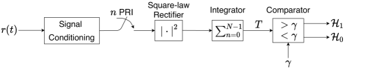
Figure 1: Non-coherent detection scheme.

 

In a non-coherent detector, the presence or absent of a target relies on the following binary hypothesis test [20]:

$$\mathcal{H}_{1}:\ T=\sum_{n=0}^{N-1}|A_{n}\exp\left(i\theta_{n}\right)+w_{n}|^{2}$$ (5a)

$$\mathcal{H}_{0}:\ T=\sum_{n=0}^{N-1}|w_{n}|^{2},$$ (5b)

where $T$ is the system’s test statistics, and $w_{n}$ is the $n$-th noise sample. The non-coherent detector scheme is depicted in Fig. 1.

Radar performance is governed by the PD and PFA. These probabilities can be computed as the probability that the decision variable $T$, defined respectively as in (5a) and (5b), falls above the decision threshold, say $\gamma$, i.e.,

$$P_{\text{D}} \triangleq\int_{\gamma}^{\infty}\mathit{f}_{T}\left(t|\mathcal{H}_{1}\right)\,\text{d}t$$ (6)

$$P_{\text{FA}} \triangleq\int_{\gamma}^{\infty}\mathit{f}_{T}\left(t|\mathcal{H}_{0}\right)\,\text{d}t.$$ (7)

Consider for the moment that $A_{n}$ is modeled as a nonfluctuating target, and that $\theta_{n}$ is modeled as sequence of independent uniformly distributed RVs, i.e., $\theta_{n}\sim\mathcal{U}\left(0,2\pi\right)$. Under these conditions, the PD is given by [1]

$$P_{\text{D}}= Q_{N}\left(\sqrt{2\zeta},\sqrt{2\gamma}\right),$$ (8)

where $Q_{(\cdot)}\left(\cdot,\cdot\right)$ is the Marcum’s Q-function [17], and

$$\zeta=\frac{1}{2\sigma^{2}}\sum_{n=0}^{N-1}\xi_{n},$$ (9)

with $\xi_{n}=A_{n}^{2}$ being the target power at the $n$-th pulse, and $2\sigma^{2}$ being the total noise power accounting for the in-phase and quadrature components. From (9), the signal-to-noise ratio (SNR) can be defined as

$$\text{SNR}= \frac{1}{2\sigma^{2}}\sum_{n=0}^{N-1}\mathbb{E}\left[\xi_{n}\right]$$

$$= \frac{1}{2\sigma^{2}}\sum_{n=0}^{N-1}\tilde{\Omega}_{n}^{\frac{1}{\tilde{\alpha}_{n}}}\Gamma\left(1+\frac{1}{\tilde{\alpha}_{n}}\right).$$ (10)

On the other hand, the PFA can be calculated as [20]

$$P_{\text{FA}}=\frac{\Gamma(N,\gamma)}{\Gamma(N)},$$ (11)

in which $\Gamma(\cdot,\cdot)$ is the incomplete gamma function [31, Eq. (8.2.1)]. In subsequent sections, we will compute the PD by allowing for Weibull target fluctuations.

IV Sum Statistics

In this section, we revisit key results on exact and approximate solutions for the sum of Weibull variates.

First, we define $\eta$ as the sum of $N$ independent RVs $\xi_{n}$, i.e.,

$$\eta=\sum_{n=0}^{N-1}\xi_{n}.$$ (12)

IV-A Exact Sum

Let $\{\xi_{n}\}_{n=0}^{N-1}$ be a set of $N$ independent and non-identically distributed (i.n.i.d) Weibull variates. The PDF of $\xi_{n}$ given by

$$f_{\xi_{n}}\left(\xi_{n}\right)=\frac{\tilde{\alpha}_{n}\xi_{n}^{\tilde{\alpha}_{n}-1}}{\tilde{\Omega}_{n}}\exp\left(-\frac{\xi_{n}^{\tilde{\alpha}_{n}}}{\tilde{\Omega}_{n}}\right),$$ (13)

where $\tilde{\alpha}_{n}>0$ is the shape parameter and $\tilde{\Omega}_{n}=\mathbb{E}\left[\xi_{n}^{\tilde{\alpha}_{n}}\right]$ is the scale parameter. In particular, for $\tilde{\alpha}_{n}=1$ and $\tilde{\alpha}_{n}=2$, (13) reduces to the Exponential and Rayleigh PDFs, respectively. Then, the PDF of (12) can be written as [21]

$$f_{\eta}\left(\eta\right)=\frac{\eta^{N-1}}{\chi^{N}\Gamma(N)}\sum_{l=0}^{\infty}\,{}_{1}F_{1}\left(N+l;N;-\frac{\eta}{\chi}\right)a_{l},\ \ \ \ \ \eta\geq 0$$ (14)

where ${}_{1}F_{1}\left(\cdot;\cdot;\cdot\right)$ is the Kummer confluent hypergeometric function [32, Eq. (13.1.2)], and the coefficients $a_{l}$ and $\chi$ are given, respectively, by

$$a_{l}=\sum_{k_{0}+\ldots+k_{N-1}=l}\prod_{n=0}^{N-1}\mathcal{V}\left(\xi_{n}\left|\frac{1}{\chi}\right.\right)$$ (15)

$$\chi=\frac{2}{N}\sum_{n=0}^{N-1}\tilde{\Omega}_{n}$$ (16)

$$\mathcal{V}\left(\xi_{n}\left|\frac{1}{\chi}\right.\right)=\sum_{k=0}^{k_{n}}\frac{(-1)^{k}\tilde{\Omega}_{n}^{\frac{k}{\tilde{\alpha}_{n}}}}{\chi^{k}k!}\binom{k_{n}}{k_{n}-k}\Gamma\left(\frac{k+\tilde{\alpha}_{n}}{\tilde{\alpha}_{n}}\right),$$ (17)

where $\sum_{k_{0}+\ldots+k_{N-1}=l}$ denotes the summation over all the possible non-negative integers $k_{0},\ldots,k_{N-1}$ satisfying the condition $k_{0}+\ldots+k_{N-1}=l$. Observe that for a proper calculation, (14) requires: 1) two infinite sums, in which one of them has to fulfill some impositions; 2) $N$ finite sums for each interaction; and 3) $N$ products for each interaction. More importantly, observe that the mathematical complexity of (14) increases as $N$ increases.

For the case of independent and identically distributed (i.i.d) Weibull variates (i.e., $\tilde{\alpha}_{n}=\tilde{\alpha}_{n},\tilde{\Omega}_{n}=\tilde{\Omega}$), the PDF of $\eta$ is still given by (21), however, the coefficients $a_{l}$ and $\chi$ are now defined, respectively, as

$$a_{l}=\sum_{k_{0}+\ldots+k_{N-1}=l}\prod_{n=0}^{N-1}\mathcal{V}\left(\xi_{n}\left|\frac{1}{\chi}\right.\right)$$ (18)

$$\chi=2\ \tilde{\Omega}$$ (19)

$$\mathcal{V}\left(\xi_{n}\left|\frac{1}{\chi}\right.\right)=\sum_{k=0}^{k_{n}}\frac{(-1)^{k}\tilde{\Omega}^{\frac{k}{\tilde{\alpha}}}}{\chi^{k}k!}\binom{k_{n}}{k_{n}-k}\Gamma\left(\frac{k+\tilde{\alpha}}{\tilde{\alpha}}\right).$$ (20)

IV-B Approximate Sum

In [25], a simple and accurate approximation for the sum of i.i.d Weibull variates was derived. The authors proposed to approximate the sum in (12) by the $\alpha$-$\mu$ envelope, given by [33]

$$f_{\eta}\left(\eta\right)=\frac{\alpha\mu^{\mu}\eta^{\alpha\mu-1}}{\Omega^{\mu}\Gamma(\mu)}\exp\left(-\frac{\mu\eta^{\alpha}}{\Omega}\right),$$ (21)

where $\alpha>0$ is the shape parameter, $\Omega=\mathbb{E}\left[\eta^{\alpha}\right]$ is the scale parameter, and $\mu=\mathbb{E}^{2}\left[\eta^{\alpha}\right]/\mathbb{V}\left[\eta^{\alpha}\right]>0$ is the inverse normalized variance of $\eta^{\alpha}$. This approximation has been anchored in the fact that the $\alpha$-$\mu$ envelope is modeled as the $\alpha$-root of the sum of i.i.d. squared Rayleigh variates, resembling somehow the algebraic structure of the exact Weibull sum, in which the $n$-th summand can be written as the $\tilde{\alpha}_{n}$-root of a squared Rayleigh variate [34].

In order to render (21) a good approximation, the moment-based estimators [35] is applied for $\Omega$, $\alpha$ and $\mu$, i.e.,

$$\frac{\mathbb{E}^{2}\left[\eta\right]}{\mathbb{E}\left[\eta^{2}\right]-\mathbb{E}^{2}\left[\eta\right]}= \frac{\Gamma^{2}(\mu+\frac{1}{\alpha})}{\Gamma(\mu)\Gamma(\mu+\frac{2}{\alpha})-\Gamma^{2}(\mu+\frac{1}{\alpha})}$$ (22)

$$\frac{\mathbb{E}^{2}\left[\eta^{2}\right]}{\mathbb{E}\left[\eta^{4}\right]-\mathbb{E}^{2}\left[\eta^{2}\right]}= \frac{\Gamma^{2}(\mu+\frac{2}{\alpha})}{\Gamma(\mu)\Gamma(\mu+\frac{4}{\alpha})-\Gamma^{2}(\mu+\frac{2}{\alpha})}$$ (23)

$$\Omega= \left[\frac{\mu^{1/\alpha}\Gamma(\mu)\mathbb{E}\left[\eta\right]}{\Gamma(\mu+\frac{1}{\alpha})}\right]^{\alpha}.$$ (24)

The exact moments $\mathbb{E}\left[\eta\right]$, $\mathbb{E}\left[\eta^{2}\right]$ and $\mathbb{E}\left[\eta^{4}\right]$ can be obtained through the multinomial expansion as [36]

$$\mathbb{E}\left[\eta^{p}\right]= \sum_{p_{1}=0}^{p}\sum_{p_{2}=0}^{p_{1}}\cdots\sum_{p_{N-2}=0}^{p_{N-3}}\binom{p}{p_{1}}\binom{p_{1}}{p_{2}}\cdots\binom{p_{N-3}}{p_{N-2}}$$

$$\times\mathbb{E}\left[\xi_{0}^{p-p_{1}}\right]\mathbb{E}\left[\xi_{1}^{p_{1}-p_{2}}\right]\cdots\mathbb{E}\left[\xi_{N-1}^{p_{N-2}}\right],$$ (25)

where $p$ is a positive integer and the required Weibull moments are given by

$$\mathbb{E}\left[\xi_{n}^{p}\right]=\tilde{\Omega}_{n}^{\frac{p}{\tilde{\alpha}_{n}}}\Gamma\left(1+\frac{p}{\tilde{\alpha}_{n}}\right).$$ (26)

V Detection Performance

In this section, we derive the PD by modeling $\xi_{n}$ as a set of i.i.d. Weibull RVs.

To do so, we first derive the PDF of $\zeta$. This can be easily obtained by performing a transformation of variables in (21), resulting in

$$\mathit{f}_{\zeta}\left(\zeta\right)=\frac{\alpha\mu^{\mu}\left(2\zeta\sigma^{2}\right)^{\alpha\mu}\exp\left(-\frac{\mu\left(2\zeta\sigma^{2}\right)^{\alpha}}{\Omega}\right)}{\zeta\Omega^{\mu}\Gamma(\mu)}.$$ (27)

Now, by using (8) and (21), the PD can be defined as

$$P_{\text{D}_{\mathcal{W}}}\triangleq\int_{0}^{\infty}Q_{N}\left(\sqrt{2\zeta},\sqrt{2\gamma}\right)\mathit{f}_{\zeta}\left(\zeta\right)\,\text{d}\zeta.$$ (28)

In order to solve (28), we start by using the Marcum’s Q-function definition [1, Eq. (15.2)]:

$$Q_{N}\left(\sqrt{2\zeta},\sqrt{2\gamma}\right)= \int_{\sqrt{2\gamma}}^{\infty}x\exp\left(-\frac{1}{2}\left(x^{2}+2\zeta\right)\right)$$

$$\times\left(\frac{x}{\sqrt{2\zeta}}\right)^{N-1}I_{N-1}\left(\sqrt{2\zeta}x\right)\,\text{d}x,$$ (29)

where $I_{(\cdot)}(\cdot)$ is modified Bessel function of the first kind [37, Eq. (03.02.02.0001.01)].

Replacing (27) and (V) in (28), yields

$$P_{\text{D}_{\mathcal{W}}}= \frac{2\alpha\mu^{\mu}\sigma^{2}\left(2\sigma^{2}\right)^{\alpha\mu-1}}{\Omega^{\mu}\Gamma(\mu)}\int_{0}^{\infty}\int_{\sqrt{2\gamma}}^{\infty}x\zeta^{\alpha\mu-1}\left(\frac{x}{\sqrt{2\zeta}}\right)^{N-1}$$

$$\times\exp\left(-\frac{1}{2}\left(2\zeta+x^{2}\right)\right)I_{N-1}\left(\sqrt{2\zeta}x\right)$$

$$\times\exp\left(-\frac{\mu\left(2\zeta\sigma^{2}\right)^{\alpha}}{\Omega}\right)\text{d}x\ \text{d}\zeta.$$ (30)

Since $\int_{0}^{\infty}|Q_{N}\left(\sqrt{2\zeta},\sqrt{2\gamma}\right)\mathit{f}_{\zeta}\left(\zeta\right)|\,\text{d}\zeta<\infty$, we can invoke the Fubini’s theorem [38] so as to interchange the order of integration, i.e.,

$$P_{\text{D}_{\mathcal{W}}}= \frac{\alpha\mu^{\mu}\left(2\sigma^{2}\right)^{\alpha\mu}}{\Omega^{\mu}\Gamma(\mu)}\int_{\sqrt{2\gamma}}^{\infty}x\exp\left(-\frac{x^{2}}{2}\right)\left(\frac{x}{\sqrt{2}}\right)^{N-1}$$

$$\times\int_{0}^{\infty}\zeta^{\alpha\mu-1-(N-1)/2}\exp(-\zeta)I_{N-1}\left(\sqrt{2\zeta}x\right)$$

$$\times\exp\left(-\frac{\mu\left(2\zeta\sigma^{2}\right)^{\alpha}}{\Omega}\right)\text{d}\zeta\ \text{d}x.$$ (31)

Now, by making use of [37, Eq. (03.02.26.0007.01)] and [37, Eq. (01.03.26.0004.01)], we can rewrite (V) as

$$P_{\text{D}_{\mathcal{W}}}= \frac{\alpha\mu^{\mu}\left(2\sigma^{2}\right)^{\alpha\mu}}{\Omega^{\mu}\Gamma(\mu)}\int_{\sqrt{2\gamma}}^{\infty}x\exp\left(-\frac{x^{2}}{2}\right)\left(\frac{x}{\sqrt{2}}\right)^{N-1}$$

$$\times\int_{0}^{\infty}\zeta^{\alpha\mu-1-(N-1)/2}\exp(-\zeta)\ i^{1-N}$$

$$\times G_{0,2}^{1,0}\left[\begin{array}[]{c}-\\ \frac{N-1}{2},\frac{1-N}{2}\\ \end{array}\left|-\frac{\zeta x^{2}}{2}\right.\right]$$ (34)

$$\times G_{1,0}^{0,1}\left[\begin{array}[]{c}-\\ 0\\ \end{array}\left|\frac{\mu\left(2\zeta\sigma^{2}\right)^{\alpha}}{\Omega}\right.\right]\text{d}\zeta\ \text{d}x,$$ (37)

where $G_{m,n}^{p,q}\left[\cdot\right]$ is the Meijer’s G-function [32, Eq. (16.17.1)].

Then, using the contour integral representation of the Meijer’s G-function [37, Eq. (07.34.02.0001.01)], along with some mathematical manipulations, we obtain

$$P_{\text{D}_{\mathcal{W}}}= \frac{\alpha\mu^{\mu}\left(2\sigma^{2}\right)^{\alpha\mu}}{\Omega^{\mu}\Gamma(\mu)}\int_{\sqrt{2\gamma}}^{\infty}x\exp\left(-\frac{x^{2}}{2}\right)\left(\frac{x}{\sqrt{2}}\right)^{N-1}$$

$$\times\left(\frac{1}{2\pi i}\right)^{2}\oint_{\ddot{\mathcal{L}}_{\textbf{s},1}}\oint_{\ddot{\mathcal{L}}_{\textbf{s},2}}\frac{i^{3N+1}\Gamma\left(s_{1}\right)\Gamma\left(\frac{N-1}{2}+s_{2}\right)}{\Gamma\left(\frac{N-1}{2}-s_{2}+1\right)}$$

$$\times\left(\frac{\mu\left(2\sigma^{2}\right)^{\alpha}}{\Omega}\right)^{-s_{1}}\left(-\frac{x^{2}}{2}\right)^{-s_{2}}\int_{0}^{\infty}\exp(-\zeta)$$

$$\times\zeta^{\alpha\mu-\alpha s_{1}-s_{2}-1-(N-1)/2}\text{d}\zeta\ \text{d}s_{1}\ \text{d}s_{2}\ \text{d}x,$$ (38)

where $\ddot{\mathcal{L}}_{\textbf{s},1}$ and $\ddot{\mathcal{L}}_{\textbf{s},2}$ are suitable contours in the complex plane.

Now, developing the inner integral and reordering the order of integration, yields

$$P_{\text{D}_{\mathcal{W}}} =\frac{\alpha\mu^{\mu}\sqrt{2}^{1-N}\left(2\sigma^{2}\right)^{\alpha\mu}}{\Omega^{\mu}\Gamma(\mu)}\left(\frac{1}{2\pi i}\right)^{2}\oint_{\dot{\mathcal{L}}_{\textbf{s},1}}\oint_{\dot{\mathcal{L}}_{\textbf{s},2}}i^{3N+1}$$

$$\times\frac{\Gamma\left(s_{1}\right)\Gamma\left(\frac{N-1}{2}+s_{2}\right)\Gamma\left(-\frac{N}{2}+\alpha\mu-\alpha s_{1}-s_{2}+\frac{1}{2}\right)}{\Gamma\left(\frac{N-1}{2}-s_{2}+1\right)}$$

$$\times\left(\frac{\mu\left(2\sigma^{2}\right)^{\alpha}}{\Omega}\right)^{-s_{1}}\left(-\frac{1}{2}\right)^{-s_{2}}$$

$$\times\int_{\sqrt{2\gamma}}^{\infty}x^{N-2s_{2}}\exp\left(-\frac{x^{2}}{2}\right)\text{d}x\ \text{d}s_{1}\ \text{d}s_{2}.$$ (39)

in which $\dot{\mathcal{L}}_{\textbf{s},1}$ and $\dot{\mathcal{L}}_{\textbf{s},2}$ are two new suitable contours. They appear since the last integration deformed the integration paths of $\ddot{\mathcal{L}}_{\textbf{s},1}$ and $\ddot{\mathcal{L}}_{\textbf{s},2}$.

TABLE I: Arguments for the Fox’s $H$-functions.

. . $\textbf{x}^{\dagger}$	$\delta^{\dagger}$	$\textbf{D}^{\dagger}$	$\beta^{\dagger}$	$\textbf{B}^{\dagger}$	$\mathcal{L}_{\textbf{s}}^{\dagger}$
$\left[\frac{\mu\left(2\sigma^{2}\right)^{\alpha}}{\Omega},-1\right]$	$\left[0,\frac{N-1}{2},\alpha\mu-\frac{N}{2}+\frac{1}{2},\frac{N}{2}+\frac{1}{2}\right]$	$\left(\begin{array}[]{cc}1&0\\ 0&1\\ -\alpha&-1\\ 0&-1\\ \end{array}\right)$	$\left[\frac{N-1}{2}+1\right]$	$\left(\begin{array}[]{cc}0&-1\\ \end{array}\right)$	$\mathcal{L}_{\textbf{s},1}^{\dagger}\times\mathcal{L}_{\textbf{s},2}^{\dagger}$
. . $\textbf{x}^{\ddagger}$	$\delta^{\ddagger}$	$\textbf{D}^{\ddagger}$	$\beta^{\ddagger}$	$\textbf{B}^{\ddagger}$	$\mathcal{L}_{\textbf{s}}^{\ddagger}$
$\left[\frac{\mu\left(2\sigma^{2}\right)^{\alpha}}{\Omega},-1,\gamma\right]$	$\left[0,\frac{N-1}{2},\alpha\mu-\frac{N}{2}+\frac{1}{2},\frac{N}{2}+\frac{1}{2},0\right]$	$\left(\begin{array}[]{ccc}1&0&0\\ 0&1&0\\ -\alpha&-1&0\\ 0&-1&1\\ 0&0&-1\\ \end{array}\right)$	$\left[\frac{N-1}{2}+1,1\right]$	$\left(\begin{array}[]{cc}0&0\\ -1&0\\ 0&-1\\ \end{array}\right)^{T}$	$\mathcal{L}_{\textbf{s},1}^{\ddagger}\times\mathcal{L}_{\textbf{s},2}^{\ddagger}\times\mathcal{L}_{\textbf{s},3}^{\ddagger}$

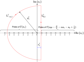
Figure 2: Integration path for $\mathcal{L}_{\textbf{s},1}^{\dagger}$.

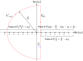
Figure 3: Integration path for $\mathcal{L}_{\textbf{s},2}^{\dagger}$.

Figure 4: Integration path for $\mathcal{L}_{\textbf{s},1}^{\ddagger}$.

Figure 5: Integration path for $\mathcal{L}_{\textbf{s},2}^{\ddagger}$.

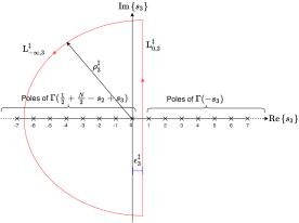
Figure 6: Integration path for $\mathcal{L}_{\textbf{s},3}^{\ddagger}$.

Finally, evaluating the remaining integral with the aid of [37, Eq. (06.06.07.0002.01)], and followed by lengthy mathematical manipulations, we obtain a closed-form solution for (28) given by

$$P_{\text{D}_{\mathcal{W}}}= \Phi\left(\textbf{H}\left[\textbf{x}^{\dagger};\delta^{\dagger};\textbf{D}^{\dagger};\beta^{\dagger};\textbf{B}^{\dagger};\mathcal{L}_{\textbf{s}}^{\dagger}\right]\right.$$

$$-\left.\textbf{H}\left[\textbf{x}^{\ddagger};\delta^{\ddagger};\textbf{D}^{\ddagger};\beta^{\ddagger};\textbf{B}^{\ddagger};\mathcal{L}_{\textbf{s}}^{\ddagger}\right]\right),$$ (40)

where $\Phi=\left(\alpha\mu^{\mu}i^{1-N}\left(2\sigma^{2}\right)^{\alpha\mu}\right)/\Omega^{\mu}\Gamma(\mu)$ and the remaining arguments of the Fox’s $H$-function are given in Table I. In addition, the integration paths for the complex contours defined in (V) are listed below:

• $\mathcal{L}_{\textbf{s},1}^{\dagger}$ is a semicircle formed by the segments $\text{L}_{0,1}^{\dagger}$ and $\text{L}_{-\infty,1}^{\dagger}$, as shown in Fig. 2, where $\rho_{1}^{\dagger}$ is the radius of the semicircle and $\epsilon_{1}^{\dagger}$ is a real that must be chosen so that all the poles of $\Gamma(s_{1})$ are separated from those of $\Gamma(\alpha\mu-\frac{N}{2}-\alpha s_{1}-s_{2}+\frac{1}{2})$.

• $\mathcal{L}_{\textbf{s},2}^{\dagger}$ is a semicircle formed by the segments $\text{L}_{0,2}^{\dagger}$ and $\text{L}_{-\infty,2}^{\dagger}$, as shown in Fig. 3, where $\rho_{2}^{\dagger}$ is the radius of the semicircle and $\epsilon_{2}^{\dagger}$ is a real that must be chosen so that all the poles of $\Gamma(\frac{N-1}{2}+s_{2})$ are separated from those of $\Gamma(\alpha\mu-\frac{N}{2}-\alpha s_{1}-s_{2}+\frac{1}{2})$ and $\Gamma(\frac{1}{2}+\frac{N}{2}-s_{2})$.

• $\mathcal{L}_{\textbf{s},1}^{\ddagger}$ is a semicircle formed by the segments $\text{L}_{0,1}^{\ddagger}$ and $\text{L}_{-\infty,1}^{\ddagger}$, as shown in Fig. 4, where $\rho_{1}^{\ddagger}$ is the radius of the semicircle and $\epsilon_{1}^{\ddagger}$ is a real that must be chosen so that all the poles of $\Gamma(s_{1})$ are separated from those of $\Gamma(\alpha\mu-\frac{N}{2}-\alpha s_{1}-s_{2}+\frac{1}{2})$.

• $\mathcal{L}_{\textbf{s},2}^{\ddagger}$ is a semicircle formed by the segments $\text{L}_{0,2}^{\ddagger}$ and $\text{L}_{-\infty,2}^{\ddagger}$, as shown in Fig. 5, where $\rho_{2}^{\ddagger}$ is the radius of the semicircle and $\epsilon_{2}^{\ddagger}$ is a real that must be chosen so that all the poles of $\Gamma(\frac{N-1}{2}+s_{2})$ are separated from those of $\Gamma(\alpha\mu-\frac{N}{2}-\alpha s_{1}-s_{2}+\frac{1}{2})$ and $\Gamma(\frac{1}{2}+\frac{N}{2}-s_{2})$ and $\Gamma(\frac{1}{2}+\frac{N}{2}-s_{2}+s_{3})$.

• $\mathcal{L}_{\textbf{s},3}^{\ddagger}$ is a semicircle formed by the segments $\text{L}_{0,3}^{\ddagger}$ and $\text{L}_{-\infty,3}^{\ddagger}$, as shown in Fig. 6, where $\rho_{3}^{\ddagger}$ is the radius of the semicircle and $\epsilon_{3}^{\ddagger}$ is a real that must be chosen so that all the poles of $\Gamma(\frac{1}{2}+\frac{N}{2}-s_{2}+s_{3})$ are separated from those of $\Gamma(-s_{3})$.

A general implementation for the multivariate Fox’s $H$-function is not yet available in mathematical packages such as MATHEMATICA, MATLAB, or MAPLE. Some works have been done to alleviate this problem [39, 40, 41]. Specifically in [39], the Fox’s $H$-function was implemented from one up to four variables. In this work, we provide an accurate and portable implementation in MATHEMATICA for the trivariate Fox’s $H$-function needed in (V). This routine can be found in Appendix A. Moreover, an equivalent series representation for (V) is also provided to ease the computation of our results. This series representation is presented in the subsequent subsection.

VI Alternative Series Representation

In this section, we derive a series representation for (V) by means of a thorough calculus of residues.

In order to apply the residue theorem [36], all the poles must lie inside the corresponding semicircles. Hence, the radius of each semicircle must tend to infinity. It can be shown that any complex integration along the paths $\text{L}_{-\infty,1}^{\dagger}$, $\text{L}_{-\infty,2}^{\dagger}$, $\text{L}_{-\infty,1}^{\ddagger}$, $\text{L}_{-\infty,2}^{\ddagger}$, and $\text{L}_{-\infty,3}^{\ddagger}$ approaches zero as $\rho_{1}^{\dagger}$, $\rho_{2}^{\dagger}$, $\rho_{1}^{\ddagger}$, $\rho_{2}^{\ddagger}$, and $\rho_{3}^{\ddagger}$ go to infinity, respectively. Therefore, the final integration paths will only include a straight lines $\text{L}_{0,1}^{\dagger}$, $\text{L}_{0,2}^{\dagger}$, $\text{L}_{0,1}^{\ddagger}$, $\text{L}_{0,2}^{\ddagger}$, and $\text{L}_{0,3}^{\ddagger}$, each of them starting at $-i\infty$ and ending at $i\infty$.

Now, we can rewrite (V) through the sum of residues [36] as in (41), shown at the top of the next page, where $\text{Res}\left[\mathcal{G}\left(a_{1},a_{2},\ldots,a_{p}\right);\left\{b_{1};b_{2};\ldots;b_{p}\right\}\right]$ denotes the residue of an arbitrary function, say $\mathcal{G}\left(a_{1},a_{2},\ldots,a_{p}\right)$, evaluated at the poles $a_{1}=b_{1}$, $a_{2}=b_{2}$, $\ldots$ , $a_{p}=b_{p}$.

$$P_{\text{D}_{\mathcal{W}}}= \Phi\left[\sum_{k,l=0}^{\infty}\text{Res}\left[\Xi_{1}\left(s_{1},s_{2}\right);\left\{-k;-l-\frac{N}{2}+\frac{1}{2}\right\}\right]-\sum_{k,l,m=0}^{\infty}\text{Res}\left[\Xi_{2}\left(s_{1},s_{2},s_{3}\right);\left\{-k;-l-\frac{N}{2}+\frac{1}{2};-l-m-N\right\}\right]\right]$$ (41)

 

In our case, the functions $\Xi_{1}$ and $\Xi_{2}$ in (41) denote the integration kernels of (V), defined , respectively, as

$$\Xi_{1}= \frac{\Gamma\left(s_{1}\right)\Gamma\left(\frac{N-1}{2}+s_{2}\right)\Gamma\left(\alpha\mu-\frac{N}{2}-\alpha s_{1}-s_{2}+\frac{1}{2}\right)}{\Gamma\left(\frac{N-1}{2}-s_{2}+1\right)}$$

$$\times\Gamma\left(\frac{N}{2}-s_{2}+\frac{1}{2}\right)\left(\frac{\mu\left(2\sigma^{2}\right)^{\alpha}}{\Omega}\right)^{-s_{1}}(-1)^{-s_{2}}$$ (42)

$$\Xi_{2}= \frac{\Gamma\left(s_{1}\right)\Gamma\left(\frac{N-1}{2}+s_{2}\right)\Gamma\left(-\frac{N}{2}+\alpha\mu-\alpha s_{1}-s_{2}+\frac{1}{2}\right)\Gamma\left(-s_{3}\right)}{\Gamma\left(1-s_{3}\right)\Gamma\left(\frac{N-1}{2}-s_{2}+1\right)}$$

$$\times\Gamma\left(\frac{N}{2}-s_{2}+s_{3}+\frac{1}{2}\right)\left(\frac{\mu\left(2\sigma^{2}\right)^{\alpha}}{\Omega}\right)^{-s_{1}}(-1)^{-s_{2}}\ \gamma^{-s_{3}}.$$ (43)

Applying the residue operation in (41), we obtain

$$P_{\text{D}_{\mathcal{W}}} =\Phi\left[\mathcal{I}_{1}-\mathcal{I}_{2}\right],$$ (44)

where $\mathcal{I}_{1}$ and $\mathcal{I}_{2}$ are summations defined, respectively, by

$$\mathcal{I}_{1}= \sum_{k,l=0}^{\infty}\frac{i^{N+1}(-1)^{k+1}\Gamma(l+k\alpha+\alpha\mu)\left(\frac{\mu\left(2\sigma^{2}\right)^{\alpha}}{\Omega}\right)^{k}}{k!\ l!}$$ (45)

$$\mathcal{I}_{2}= \sum_{k,l,m=0}^{\infty}\frac{i^{N+1}(-1)^{k+m+1}\gamma^{l+m+N}\Gamma(l+m+N)}{k!\ l!\ m!\ \Gamma(l+N)\Gamma(l+m+N+1)}$$

$$\ \ \ \times\Gamma(l+k\alpha+\alpha\mu)\left(\frac{\mu\left(2\sigma^{2}\right)^{\alpha}}{\Omega}\right)^{k}.$$ (46)

For convenience, we start by solving $\mathcal{I}_{2}$. Using [42, Eq. (5.2.8.1)] and [32, Eq. (5.5.1)], followed by lengthy mathematical manipulations, we can express (VI) as

$$\mathcal{I}_{2} =\sum_{k,l=0}^{\infty}\frac{i^{N+1}(-1)^{k+2l+1}\Gamma(l+k\alpha+\alpha\mu)\left(\frac{\mu\left(2\sigma^{2}\right)^{\alpha}}{\Omega}\right)^{k}}{k!\ l!}$$

$$- \sum_{k,l=0}^{\infty}\frac{i^{N+1}(-1)^{k+1}\Gamma(l+k\alpha+\alpha\mu)\Gamma(l+N,\gamma)\left(\frac{\mu\left(2\sigma^{2}\right)^{\alpha}}{\Omega}\right)^{k}}{k!\ l!\ \Gamma(l+N)}$$ (47)

Note that the first series in (VI) is identical to $\mathcal{I}_{1}$; hence, they will cancel each other. Then, after minor simplifications, we finally obtain

$$P_{\text{D}_{\mathcal{W}}} =\frac{\alpha\Psi^{\mu}}{\Gamma(\mu)}\sum_{k,l=0}^{\infty}\frac{\Gamma(l+N,\gamma)\Gamma(l+k\alpha+\alpha\mu)\left(-\Psi\right)^{k}}{k!\ l!\ \Gamma(l+N)},$$ (48)

where $\Psi=\mu\left(2\sigma^{2}\right)^{\alpha}/\Omega$. It is worth mentioning that (48) is also an original contribution of this work, enjoying a low computational burden as compared to [20, Eq. 30].

VII Sample Numerical Results

Input: $\tilde{\alpha}_{n}$, $\tilde{\Omega}_{n}$ and $N$

1 Do: Compute the moments of $\eta$ and $\xi_{n}$ by using Eqs. (IV-B) and (26).

2 Do: Solve numerically the parameters $\alpha$, $\mu$ and $\Omega$ by using Eqs. (22)–(24).

3 Do: Apply Eq. (V) or, alternatively, Eq. (48).

Output: $P_{\text{D}_{\mathcal{W}}}$

Algorithm 1 Computation of $P_{\text{D}_{\mathcal{W}}}$

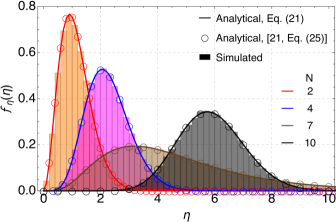
Figure 7: PDF of $\eta$ for $\tilde{\Omega}_{n}=1/2$, $\tilde{\alpha}_{n}=3/2$, and different values of $N$.

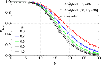
Figure 8: $P_{\text{D}_{\mathcal{W}}}$ versus $\gamma$ for $\tilde{\Omega}_{n}=13/10$, $\sigma_{0}^{2}=1$, $N=10$ and different values of $\tilde{\alpha}_{n}$.

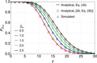
Figure 9: $P_{\text{D}_{\mathcal{W}}}$ versus $\gamma$ for $\tilde{\alpha}_{n}=2$, $\sigma_{0}^{2}=1$, $N=10$ and different values of $\tilde{\Omega}_{n}$.

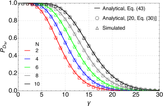
Figure 10: $P_{\text{D}_{\mathcal{W}}}$ versus $\gamma$ for $\tilde{\alpha}_{n}=3$, $\tilde{\Omega}_{n}=2$, $\sigma_{0}^{2}=1$ and different values of $N$.

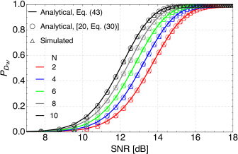
Figure 11: $P_{\text{D}_{\mathcal{W}}}$ versus SNR for different values of $N$.

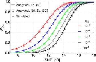
Figure 12: $P_{\text{D}_{\mathcal{W}}}$ versus SNR for different values $P_{\text{FA}}$.

TABLE II: Efficiency of (48) as compared to [20, Eq. (30)].

Parameter Settings	$P_{\text{D}_{\mathcal{W}}}$ $[\%]$	$\mathcal{T}$	Computation Time for [20, Eq. (30)] [$s$]	Computation Time for Eq. (48) [$s$]	Time saving [%]
$N=3$, $\tilde{\alpha}_{n}=1/2$, $\tilde{\mu}_{n}=3/2$, $\tilde{\Omega}_{n}=2$, $\sigma^{2}=1$, $\gamma=3$	$69.1485$	$15.34$ $\times 10^{-4}$	$1341.64$	$27.2091$	$97.9721$
$N=3$, $\tilde{\alpha}_{n}=1$, $\tilde{\mu}_{n}=1$, $\tilde{\Omega}_{n}=2$, $\sigma^{2}=1$, $\gamma=2$	$83.1095$	$11.14$ $\times 10^{-4}$	$1543.54$	$45.0135$	$97.0837$
$N=3$, $\tilde{\alpha}_{n}=1/2$, $\tilde{\mu}_{n}=2$, $\tilde{\Omega}_{n}=5$, $\sigma^{2}=1$, $\gamma=3$	$88.7412$	$32.44$ $\times 10^{-4}$	$1711.14$	$43.9077$	$97.4341$
$N=5$, $\tilde{\alpha}_{n}=1/2$, $\tilde{\mu}_{n}=3/2$, $\tilde{\Omega}_{n}=2$, $\sigma^{2}=1$, $\gamma=2$	$97.6474$	$49.13$ $\times 10^{-4}$	$1579.19$	$26.4729$	$98.3236$
$N=5$, $\tilde{\alpha}_{n}=1/2$, $\tilde{\mu}_{n}=1$, $\tilde{\Omega}_{n}=2$, $\sigma^{2}=1$, $\gamma=2$	$90.2578$	$88.12$ $\times 10^{-4}$	$1613.22$	$46.2803$	$97.1312$
$N=5$, $\tilde{\alpha}_{n}=1$, $\tilde{\mu}_{n}=1/2$, $\tilde{\Omega}_{n}=5$, $\sigma^{2}=1$, $\gamma=2$	$97.5109$	$57.58$ $\times 10^{-4}$	$1887.91$	$46.9172$	$97.5149$
$N=5$, $\tilde{\alpha}_{n}=1/3$, $\tilde{\mu}_{n}=3$, $\tilde{\Omega}_{n}=2$, $\sigma^{2}=1$, $\gamma=2$	$92.0891$	$92.33$ $\times 10^{-4}$	$1787.32$	$48.5396$	$97.2842$
$N=6$, $\tilde{\alpha}_{n}=1/4$, $\tilde{\mu}_{n}=3$, $\tilde{\Omega}_{n}=1$, $\sigma^{2}=1$, $\gamma=1$	$99.9091$	$19.82$ $\times 10^{-4}$	$1923.67$	$46.0083$	$97.6083$
$N=6$, $\tilde{\alpha}_{n}=1/5$, $\tilde{\mu}_{n}=2$, $\tilde{\Omega}_{n}=1/2$, $\sigma^{2}=1$, $\gamma=1$	$99.9387$	$22.32$ $\times 10^{-4}$	$1829.53$	$48.4967$	$97.3492$
$N=5$, $\tilde{\alpha}_{n}=1/2$, $\tilde{\mu}_{n}=3/2$, $\tilde{\Omega}_{n}=2$, $\sigma^{2}=1$, $\gamma=3$	$99.9413$	$67.12$ $\times 10^{-4}$	$1876.83$	$51.5077$	$97.2556$

In this section, we corroborate the validity of our expressions through Monte-Carlo simulations and numerical integration. In addition, we illustrate the accuracy and low computational burden of (48). Here, $P_{\text{D}_{\mathcal{W}}}$ was computed by performing the three steps described in Algorithm 1.

Fig. 7 shows the analytical and simulated PDF of $\eta$. The PDF parameters have been selected to show the wide range of shapes that the PDF can exhibit. Note the perfect agreement between the approximation proposed in [25], the exact formulation in [21], and Monte-Carlo simulations.

Figs. 8–10 show $P_{\text{D}_{\mathcal{W}}}$ versus $\gamma$ by varying $\tilde{\alpha}_{n}$, $\tilde{\Omega}_{n}$ and $N$. In all cases, observe the outstanding accuracy between our derived expressions and [20, Eq. (30)]. Also, note that the detection performance improves as $\tilde{\Omega}_{n}$ and $N$ increase, as expected. Similarly, the detection improves as $\tilde{\alpha}_{n}$ is reduced.

Fig. 11 shows $P_{\text{D}_{\mathcal{W}}}$ versus SNR for different values of $N$. Note that for a fixed SNR, the higher the number of antennas, the better the radar detection. For example, given a $\text{SNR}=14$ dB, we obtain $P_{\text{D}_{\mathcal{W}}}=0.61,0.73,0.83,0.91,0.94$ for $N=2,4,6,8,10$, respectively.

Fig. 12 shows $P_{\text{D}_{\mathcal{W}}}$ versus SNR for different values of $P_{\text{FA}}$. Note that the radar performance improves as $P_{\text{FA}}$ is increased. This fundamental trade-off means that if $P_{\text{FA}}$ is reduced, $P_{\text{D}_{\mathcal{W}}}$ decreases as well. For example, given a $\text{SNR}=14$ dB, we obtain $P_{\text{D}_{\mathcal{W}}}=0.48,0.59,0.76,0.86,0.95$ for $P_{\text{FA}}=10^{-7},10^{-6},10^{-5},10^{-4},10^{-3}$, respectively.

Now, we evaluate the efficiency of (48). In order to so, we define 10 parameter settings, each with its corresponding $P_{\text{D}_{\mathcal{W}}}$, truncation error and the associated time saving to achieve the same accuracy goal imposed to [20, Eq. (6)], say, around $10^{-4}$, as shown in Table II. The truncation error is expressed as

$$\mathcal{T}=|P_{\text{D}_{\mathcal{W}}}-\overline{P_{\text{D}_{\mathcal{W}}}}|,$$ (49)

where $\overline{P_{\text{D}_{\mathcal{W}}}}$ is the probability of detection obtained via the numerical integration of [20, Eq. (6)]. Observe that across all scenarios, the computation time dropped dramatically, showing an impressive reduction above $97$%. Moreover, (48) requires less than 275 terms to guarantee a truncation error of about $10^{-4}$.

VIII Conclusions

In this paper, we derived a highly accurate approximation for the PD of a non-coherent detector operating with Weibull fluctuation targets. This approximation is given in terms of both a closed-form expression and a fast converging series. Numerical results and Monte-Carlo simulations corroborated the validity of our expressions, and showed the accuracy and fast rate of convergence of our results. For instance, our series representation proved to be more tractable and faster than  [20, Eq. (30)], showing an impressive reduction in computation time (above $97$%) and in the required number of terms (less than 275 terms) to guarantee a truncation error of about $10^{-4}$. The contributions derived herein allow us to reduce the computational burden that demands the PD evaluation. Moreover, they can be quickly executed on an ordinary desktop computer, serving as a useful tool for radar designers.

Appendix A Mathematica Implementation for the Trivariate Fox H-Function

⬇ ClearAll["Global‘*"]; Remove[s]; H[x_, delta_, D_,beta_, B_] := Module[{UpP,LoP,Theta,R1,T1,R2,T2,m,n}, L=Length[Transpose[D]]; m=Length[D]; (*Number of Gamma functions in the numerator*) n=Length[B]; (*Number of Gamma functions in the denominator*) S=Table[Subscript[s,i],{i,1,L}]; (*s is the vector containing the number of branches, in our case s=[s_1,s_2,s_3]*) UpP=Product[Gamma[delta[[1,j]]+Sum[D[[j,k]] S[[k]],{k,1, L}]], {j,1,m}]; LoP=Product[Gamma[beta[[1,j]]+Sum[B[[j,k]] S[[k]],{k,1,L}]],{j,1,n}]; Theta=UpP/LoP (*Theta computes Eq. (2)*); W=50; (*Limit for the complex integration. Increase "MaxRecursion" for large W.*) T=Table[delta[[1,j]]+Sum[D[[j,k]] S[[k]],{k,1,L}]>0,{j,1,m}]; (*Generation of the restriction table*) limit1 = -1(*Minimum limit of recursion*); limit2 = 1(*Maximum limit of recursion*); spacing = 1/2; T1=T/.{Subscript[s,1]->eps1,Subscript[s,2] ->eps2,Subscript[s,3]->eps3}; Do[eps1=i;Do[eps2=j;Do[eps3=k; flag1=If[Total[Boole[T1]]==m,1,0]; If[Total[T1]==m,Break[]], {k,limit1,limit2,spacing}]; If[flag1==1,Break[]], {j,limit1,limit2,spacing}]; If[flag1==1,Break[]], {i,limit1,limit2,spacing}]; (*Find eps1, eps2 and eps3, nedded to separate the poles of left in Eq. (2), from those of the right.*) kernel=Theta(x[[1]])^(-S[[1]])(x[[2]]) ^(-S[[2]]) (x[[3]])^(-S[[3]]) /.{S[[1]]->s1,S[[2]]->s2,S[[3]]->s3}; (*Construction of the integratiion kernel*) Result= N[1/(2*Pi*I)^2 NIntegrate[kernel, {s1,-W-eps1*I,1/2-eps1*I}, {s2,-W-eps2*I,1/2-eps2*I}, {s3,-W-eps3*I,1/2-eps3*I}, Method->{"GlobalAdaptive", Method->{"GaussKronrodRule"}, "MaxErrorIncreases"->1000}, MaxRecursion->20,AccuracyGoal->5, WorkingPrecision->20],20]; Print[""Result""]];

References

- [1] M. A. Richards, J. Scheer, W. A. Holm, and W. L. Melvin, Principles of Modern Radar: Basic Principles, 1st ed. West Perth, WA, Australia: SciTech, 2010.
- [2] M. A. Richards, Fundamentals of Radar Signal Processing, 2nd ed. Ney York, NY, USA: McGraw-Hill, 2014.
- [3] W. A. Skiliman, “Comments on “On the derivation and numerical evaluation of the Weibull-Rician distribution”,” IEEE Trans. Aerosp. Electron. Syst., vol. AES-21, no. 3, pp. 427–429, May 1985.
- [4] P. Swerling, “Probability of detection for fluctuating targets,” IRE Transactions on Information Theory, vol. IT-6, pp. 269–308, Apr. 1960.
- [5] D. A. Shnidman, “Radar detection probabilities and their calculation,” IEEE Trans. Aerosp. Electron. Syst., vol. 31, no. 3, pp. 928–950, Jul. 1995.
- [6] ——, “Expanded swerling target models,” IEEE Trans. Aerosp. Electron. Syst., vol. 39, no. 3, pp. 1059–1069, Jul. 2003.
- [7] D. A. Shnidman, “Binary integration for Swerling target fluctuations,” IEEE Trans. Aerosp. Electron. Syst., vol. 34, no. 3, pp. 1043–1053, Jul. 1998.
- [8] H. Lim and D. Yoon, “Refinements of binary integration for Swerling target fluctuations,” IEEE Trans. Aerosp. Electron. Syst., vol. 55, no. 2, pp. 1032–1036, July 2019.
- [9] D. K. Barton, Radar Equations for Modern Radar, 1st ed. Massachusetts, MA, USA: Artech House, 2013.
- [10] B. R. Mahafza, Radar Systems Analysis and Design Using Matlab, 3rd ed. CRC Press, 2013.
- [11] M. A. Weiner, “Detection probability for partially correlated Chi-square targets,” IEEE Trans. Aerosp. Electron. Syst., vol. 24, no. 4, pp. 411–416, Jul. 1988.
- [12] I. Kanter, “Exact detection probability for partially correlated Rayleigh targets,” IEEE Trans. Aerosp. Electron. Syst., vol. AES-22, no. 2, pp. 184–196, Mar. 1986.
- [13] D. A. Shnidman, “Generalized radar clutter model,” IEEE Trans. Aerosp. Electron. Syst., vol. 35, no. 3, pp. 857–865, Jul. 1999.
- [14] M. Sekine, S. Ohtani, T. Musha, T. Irabu, E. Kiuchi, T. Hagisawa, and Y. Tomita, “Weibull-distributed ground clutter,” IEEE Trans. Aerosp. Electron. Syst., vol. AES-17, no. 4, pp. 596–598, Jul. 1981.
- [15] D. C. Schleher, “Radar detection in Weibull clutter,” IEEE Trans. Aerosp. Electron. Syst., vol. AES-12, no. 6, pp. 736–743, Nov. 1976.
- [16] S. M. Kay, Fundamentals of Statistical Signal Processing: Estimation Theory, 1st ed. New Jersey, NJ, USA: Prentice Hall PTR, 1993.
- [17] ——, Fundamentals of Statistical Signal Processing: Detection Theory, 2nd ed. New Jersey, NJ, USA: Prentice Hall PTR, 1998.
- [18] L. V. Blake, Radar Range-performance Analysis, 1st ed. Norwood, MA, USA: Artech House, 1986.
- [19] G. Cui, A. D. Maio, and M. Piezzo, “Performance prediction of the incoherent radar detector for correlated generalized swerling-chi fluctuating targets,” IEEE Trans. Aerosp. Electron. Syst., vol. 49, no. 1, pp. 356–368, Jan. 2013.
- [20] G. Cui, A. D. Maio, V. Carotenuto, and L. Pallotta, “Performance prediction of the incoherent detector for a Weibull fluctuating target,” IEEE Trans. Aerosp. Electron. Syst., vol. 50, no. 3, pp. 2176–2184, Dec. 2014.
- [21] F. Yilmaz and M. S. Alouini, “Sum of Weibull variates and performance of diversity systems,” in Proc. International Wireless Communications and Mobile Computing Conference (IWCMC’09), Leipzig, Germany, Jun. 2009, p. 247–252.
- [22] M. You, H. Sun, J. Jiang, and J. Zhang, “Effective rate analysis in Weibull fading channels,” IEEE Wireless Commun. Lett., vol. 5, no. 4, pp. 340–343, Apr. 2016.
- [23] C. H. M. de Lima, H. Alves, and P. H. J. Nardelli, “Fox -function: A study case on variate modeling of dual-hop relay over Weibull fading channels,” in 2018 IEEE Wireless Communications and Networking Conference (WCNC), Apr. 2018, pp. 1–5.
- [24] Y. Abo Rahama, M. H. Ismail, and M. S. Hassan, “On the sum of independent Fox’s -function variates with applications,” IEEE Trans. Veh. Technol., vol. 67, no. 8, pp. 6752–6760, Aug. 2018.
- [25] J. C. S. Santos Filho and M. D. Yacoub, “Simple precise approximations to Weibull sums,” IEEE Commun. Lett., vol. 10, no. 8, pp. 614–616, Aug. 2006.
- [26] C. R. N. Da Silva, N. Simmons, E. J. Leonardo, S. L. Cotton, and M. D. Yacoub, “Ratio of two envelopes taken from –, –, and – variates and some practical applications,” IEEE Access, vol. 7, pp. 54 449–54 463, May 2019.
- [27] F. D. A. García, H. R. C. Mora, G. Fraidenraich, and J. C. S. Santos Filho, “Square-law detection of exponential targets in Weibull-distributed ground clutter,” IEEE Geosci. Remote Sens. Lett., to be published, doi: 10.1109/LGRS.2020.3009304.
- [28] C. R. N. da Silva, E. J. Leonardo, and M. D. Yacoub, “Product of two envelopes taken from –, – , and – distributions,” IEEE Trans. Commun., vol. 66, no. 3, pp. 1284–1295, Nov. 2018.
- [29] N. T. Hai and H. M. Srivastava, “The convergence problem of certain multiple Mellin-Barnes contour integrals representing H-functions in several variables,” Computers & Mathematics with Applications, vol. 29, no. 6, pp. 17–25, 1995.
- [30] F. D. A. García, H. R. C. Mora, G. Fraidenraich, and J. C. S. Santos Filho, “Alternative representations for the probability of detection of non-fluctuating targets,” Electron. Lett., vol. 56, no. 21, pp. 1136–1139, Oct. 2020.
- [31] M. Abramowitz and I. A. Stegun, Handbook of Mathematical Functions with Formulas, Graphs, and Mathematical Tables, 10th ed. Washington, DC: US Dept. of Commerce: National Bureau of Standards, 1972.
- [32] F. W. J. Olver, D. W. Lozier, R. F. Boisvert, and C. W. Clark, NIST Handbook of Mathematical Functions, 1st ed. Washington, DC: US Dept. of Commerce: National Institute of Standards and Technology (NIST), 2010.
- [33] M. D. Yacoub, “The - distribution: A physical fading model for the stacy distribution,” IEEE Trans. Veh. Technol., vol. 56, no. 1, pp. 27–34, Jan. 2007.
- [34] ——, “The - distribution: a general fading distribution,” in Proc. 13th IEEE Int. Symp. Pers., Indoor Mobile Radio Commun., vol. 2, Sept. 2002, p. 629–633.
- [35] A. Papoulis, Probability, Random Variables, and Stochastic Processes, 4th ed. Ney York, NY, USA: McGraw-Hill, 2002.
- [36] E. Kreyszig, Advanced Engineering Mathematics, 10th ed. New Jersey, NJ, USA: John Wiley & Sons, 2010.
- [37] Wolfram Research, Inc. (2018), Wolfram Research, Accessed: Sept. 19, 2020. [Online]. Available: http://functions.wolfram.com
- [38] G. Fubini, “Sugli integrali multipli.” Rom. Acc. L. Rend. (5), vol. 16, no. 1, pp. 608–614, 1907.
- [39] H. R. Alhennawi, M. M. H. E. Ayadi, M. H. Ismail, and H. A. M. Mourad, “Closed-form exact and asymptotic expressions for the symbol error rate and capacity of the H-function fading channel,” IEEE Trans. Veh. Technol., vol. 65, no. 4, pp. 1957–1974, Apr. 2016.
- [40] F. D. G. Almeida, A. C. F. Rodriguez, G. Fraidenraich, and J. C. S. Santos Filho, “CA-CFAR detection performance in homogeneous Weibull clutter,” IEEE Geosci. Remote Sens. Lett., vol. 16, no. 6, pp. 887–891, Jun. 2019.
- [41] F. Yilmaz and M. S. Alouini, “Product of the powers of generalized nakagami- variates and performance of cascaded fading channels,” in Proc. IEEE Global Telecommun. Conf. (GLOBECOM), Abu Dhabi, UAE, Nov. 2009, pp. 1–8.
- [42] A. P. Prudnikov, Y. A. Bryčkov, and O. I. Maričev, Integral and Series: Vol. 2, 2nd ed., Fizmatlit, Ed. Moscow, Russia: Fizmatlit, 1992.