Quadrature error estimates for layer potentials evaluated near curved surfaces in three dimensions

Abstract

The quadrature error associated with a regular quadrature rule for evaluation of a layer potential increases rapidly when the evaluation point approaches the surface and the integral becomes nearly singular. Error estimates are needed to determine when the accuracy is insufficient and a more costly special quadrature method should be utilized.

The final result of this paper are such quadrature error estimates for the composite Gauss-Legendre rule and the global trapezoidal rule, when applied to evaluate layer potentials defined over smooth curved surfaces in $\mathbb{R}^{3}$. The estimates have no unknown coefficients and can be efficiently evaluated given the discretization of the surface, invoking a local one-dimensional root-finding procedure. They are derived starting with integrals over curves, using complex analysis involving contour integrals, residue calculus and branch cuts. By complexifying the parameter plane, the theory can be used to derive estimates also for curves in $\mathbb{R}^{3}$. These results are then used in the derivation of the estimates for integrals over surfaces. In this procedure, we also obtain error estimates for layer potentials evaluated over curves in $\mathbb{R}^{2}$. Such estimates combined with a local root-finding procedure for their evaluation were earlier derived for the composite Gauss-Legendre rule for layer potentials written in complex form [4]. This is here extended to provide quadrature error estimates for both complex and real formulations of layer potentials, both for the Gauss-Legendre and the trapezoidal rule.

Numerical examples are given to illustrate the performance of the quadrature error estimates. The estimates for integration over curves are in many cases remarkably precise, and the estimates for curved surfaces in $\mathbb{R}^{3}$ are also sufficiently precise, with sufficiently low computational cost, to be practically useful.

1 Introduction

Accurate evaluation of layer potentials is crucial when solving partial differential equations using boundary integral methods. When an evaluation point is close to the boundary, the integral defining such a layer potential has a rapidly varying integrand. A regular quadrature method will then yield large errors, and a specialized quadrature method must be used to keep errors low. There is a variety of specialized quadrature methods, but the increased accuracy that they can provide comes at an additional computational cost. It is therefore desireable to have error estimates for the regular quadrature method that can be used to determine when the accuracy will be insufficient and a special quadrature method must be applied.

In this paper, we study the errors incurred when using two quadrature methods that are commonly applied to evaluate layer potentials: the panel based Gauss-Legendre quadrature rule and the global trapezoidal rule. The simplest example of a layer potential in 3D is the harmonic single layer potential

$$S^{3D}_{H}[\sigma](\bm{x})=\int_{S}\frac{\sigma(\bm{y})}{\mathinner{\!\left\lVert\bm{y}-\bm{x}\right\rVert}}\,\,\operatorname{d\!}S(\bm{y}),$$ (1)

but we will consider the more generic form

$$u(\bm{x})=\int_{S}\frac{k\left(\bm{x},\bm{y}\right)\sigma(\bm{y})}{\mathinner{\!\left\lVert\bm{y}-\bm{x}\right\rVert}^{2p}}\operatorname{d\!}S(\bm{y}),\quad p=1/2,3/2,\ldots$$ (2)

where $k\left(\bm{x},\bm{y}\right)$ and $\sigma(\bm{y})$ are assumed to be smooth, and the evaluation point $\bm{x}\in\mathbb{R}^{3}$ can be arbitrarily close to, but not on, the surface $S$. The surface $S$ in $\mathbb{R}^{3}$, is supposed to be smooth over each separate section (panel or other) that a quadrature rule will be applied to.

Layer potentals in 2D can also be written in the generic form (2). Here, $S$ is now instead a curve in $\mathbb{R}^{2}$, and $p=1,2,3,\ldots$. An example is the harmonic double layer potential, in 2D given by (with $\bm{n}_{y}$ the normal vector at $\bm{y}\in S$),

$$D^{2D}_{H}[\sigma](\bm{x})=\int_{S}\sigma(\bm{y})\frac{{\bm{n}_{y}}\cdot(\bm{y}-\bm{x})}{\mathinner{\!\left\lVert\bm{y}-\bm{x}\right\rVert}^{2}}\,\,\operatorname{d\!}S(\bm{y}).$$

Now, let $\bm{y}^{*}$ be the closest point to $\bm{x}$ on $S$. The closer $\bm{x}$ is to $S$, the more preaked the integrand in (2) will become around $\bm{y}^{*}$ due to the factor $\mathinner{\!\left\lVert\bm{y}-\bm{x}\right\rVert}^{-2p}$. Analytically, the integral is well defined, but numerically it will be difficult to approximate well. Following the terminology of Elliott et al., [6, 7, 8, 9], we will henceforth call this a nearly singular integral.

To start with the basics, consider a simple example of a 1D-integral

$$\int_{-1}^{1}\frac{1}{t^{2}+b^{2}}\,dt,$$

which will be nearly singular when $b>0$ is small. We can e.g. apply an $n$-point Gauss-Legendre quadrature rule to approximate this integral. The error will be large when $b$ is small, but decrease exponentially with increasing values of $b$. The classical error estimate, available in e.g. Abramowitz and Stegun [1, eq. 25.4.30] or in the DLMF [15, §3.5(v)], includes the $2n^{th}$ derivative of the integrand, and will largely over estimate the error [3, sec. 3.1.1].

The above integral can be written in the following form (with $a=0$, $p=1$)),

$$\int_{-1}^{1}\frac{1}{\left((t-a)^{2}+b^{2}\right)^{p}}\,dt=\int_{-1}^{1}\frac{1}{\left(t-z_{0}\right)^{p}\left(t-\bar{z}_{0}\right)^{p}}\,dt,\quad z_{0}=a+ib,\quad a\in\mathbb{R},b>0,p\in{\mathbb{Z}}^{+}.$$ (3)

Here, it is clear that with $b$ small, the integrand has poles in the complex plane close to the integration interval along the real axis. Donaldson and Elliott [6] introduced a theory that defines the quadrature error as a contour integral in the complex plane over the integrand multiplied with a so-called remainder function, that depends on the quadrature rule. Using residue calculus for this meromorphic integrand, Elliott et al. [7] derived an error estimate for the error in the approximation of (3) for $p=1$ with an $n$-point Gauss-Legendre quadrature rule. Later, af Klinteberg and Tornberg [3] derived error estimates for a general positive integer $p$. In [3], results were also derived for the trapezoidal rule (hence with a different remainder function), considering integration over the unit circle rather than an open interval.

Error estimates were also derived for the $n$-point Gauss-Legendre quadrature rule by af Klinteberg and Tornberg in [3] for integrals in the form

$$\int_{-1}^{1}\frac{1}{\left(t-z_{0}\right)^{p}}\,dt,\quad z_{0}=a+ib,\quad a\in\mathbb{R},b\neq 0,p\in{\mathbb{Z}}^{+}.$$ (4)

In 2D, it is convenient to rewrite layer potentials using complex variables. A typical form of integrals to evaluate over one segment of the curve is

$$\int_{-1}^{1}\frac{f(t)\,\gamma^{\prime}(t)}{(\gamma(t)-z_{0})^{p}}\,dt,$$ (5)

where $\gamma(t)\in\mathbb{C}$ is a parameterization of the curve segment, which is assumed to be smooth. In [4], af Klinteberg and Tornberg derived the quadrature error estimate for the Gauss-Legendre method as applied to (5) for $p\in{\mathbb{Z}}^{+}$. Generalization of the error estimates for “flat panels” (4) to curved segments (5) introduces a geometry factor. Evaluation of the estimates requires the knowledge of $t_{0}\in\mathbb{C}$ such that $\gamma(t_{0})=z_{0}$. A numerical procedure is introduced to compute $t_{0}$, given the Gauss-Legendre points used to discretize the panel.

The harmonic double layer potential can be written in the form (5) with $p=1$. In the combined field Helmholtz potential, Hankel functions are present, and additional steps are needed in the derivation of the error estimates. In both cases, the resulting estimates are remarkably accurate, when combined with the numerical procedure to compute $t_{0}$ [4]. Using the same techniques, error estimates for Stokes layer potentials are derived in [16], again with excellent results.

Evaluations of integrals in the form (5) with larger $p$ are required to obtain expansion coefficients in the “Quadrature by Expansion” method (QBX) [11]. In [4], the derived error estimates were used to control the coefficient error in the expansions, in the framework of an adaptive QBX method applied to evaluate the harmonic double layer potential and the combined field Helmholtz potential. This way, automatic parameter selection in order to fulfil a desired accuracy was facilitated.

The integral in (3) (or (4) if using a formulation in complex variables) is the simplest prototype integral that can be related to an integral over a segment of a curve. Considering instead a patch of a 3D surface, the simplest two-dimensional integral to consider is

$$\int_{-1}^{1}\int_{-1}^{1}\frac{ds\,dt}{\left((t-a)^{2}+s^{2}+b^{2}\right)^{p}}\quad a\in\mathbb{R},b>0.$$ (6)

Elliott et al. [8] studied the approximation of this integral with an $n_{s}\times n_{t}$ tensor product Gauss-Legendre rule. They derived error estimates for the two cases with $p=1$ and $p=1/2$, the latter for $a=0$. This error analysis was further extended in [9], including a higher order error term that was previously neglected. Considering such tensor product Gauss-Legendre rules, af Klinteberg and Tornberg [3], derived quadrature error estimates for QBX coefficients evaluated over flat 2D patches. A similar estimate was also derived for the case of a spheroidal surface, discretized with a tensor product rule with the trapezoidal rule in the (periodic) azimuthal angle and the Gauss-Legendre rule in the polar angle.

In [14], Morse et al. derives an error estimate for the evaluation of the double layer potential over a general surface in 3D discretized with quadrilateral patches and a tensor product Clenshaw-Curtis quadrature rule. The estimate however contains high derivatives of the Green’s function which makes it difficult to evaluate and hence, as the author acknowledges, cannot really be applied. In this paper we aim to provide error estimates without unknown coefficients that can rapidly be evaluated. They can then be directly applied to determine e.g. when a regular quadrature rule is insufficient or how large upsampling is needed.

2 Contributions and outline

In this paper, we derive estimates for the numerical errors that results when applying quadrature rules to nearly singular integrals. Specifically, we consider Gauss-Legendre (panel based) and trapezoidal (global) approximations for evaluation of integrals of the type

$$u(\bm{x})=\int_{S}\frac{k\left(\bm{x},\bm{y}\right)\sigma(\bm{y})}{\mathinner{\!\left\lVert\bm{y}-\bm{x}\right\rVert}^{2p}}\operatorname{d\!}S(\bm{y}),$$ (7)

where $\bm{x}$ can be close to, but not on, $S$. We assume the functions $k\left(\bm{x},\bm{y}\right)$ and $\sigma(\bm{y})$ as well as $S$ to be smooth and derive error estimates for $2p\in{\mathbb{Z}}^{+}$ for the following cases:

1. $S$ is a curve in $\mathbb{R}^{2}$ or $\mathbb{R}^{3}$ that we denote $\Gamma$, where $\Gamma=\gamma(E)$, $E\subset\mathbb{R}$.

   In this case, we can write the layer potential in (7) in the equivalent form

   $$u(\bm{x})=\int_{E}\frac{k\left(\bm{x},\bm{\gamma}(t)\right)\sigma(\bm{\gamma}(t))}{\mathinner{\!\left\lVert\bm{\gamma}(t)-\bm{x}\right\rVert}^{2p}}\mathinner{\!\left\lVert\bm{\gamma}^{\prime}(t)\right\rVert}\operatorname{d\!}t=\int_{E}\frac{f(t)\operatorname{d\!}t}{\mathinner{\!\left\lVert\bm{\gamma}(t)-\bm{x}\right\rVert}^{2p}},$$ (8)

   where we in the last step have collected all the components that are assumed to be smooth into the function $f(t)$, which has an implicit dependence on $\bm{x}$.

2. $S$ is a two-dimensional surface in $\mathbb{R}^{3}$, parameterized by $\bm{\gamma}\mathrel{\mathop{\ordinarycolon}}E\rightarrow\mathbb{R}^{3}$, $E=\left\{E_{1}\times E_{2}\right\}\subset\mathbb{R}^{2}$. Now, the prototype layer potential (7) takes the form

   $$u(\bm{x})=\iint_{E}\frac{k\left(\bm{x},\bm{\gamma}(s,t)\right)\sigma(\bm{\gamma}(s,t))}{\mathinner{\!\left\lVert\bm{\gamma}(s,t)-\bm{x}\right\rVert}^{2p}}\mathinner{\!\left\lVert\mathinner{\dfrac{\partial{}\bm{\gamma}}{\partial{s}}}\times\mathinner{\dfrac{\partial{}\bm{\gamma}}{\partial{t}}}\right\rVert}\operatorname{d\!}t\operatorname{d\!}s=\iint_{E}\frac{f(s,t)\operatorname{d\!}t\operatorname{d\!}s}{\mathinner{\!\left\lVert\bm{\gamma}(s,t)-\bm{x}\right\rVert}^{2p}}.$$ (9)

   Here we have again collected all the smooth components into the function $f(s,t)$, which depends implicitly on $\bm{x}$.

It is possible to derive error estimates also for kernels with a logarithmic singularity [7], relevant for 2D problems. However we are interested in error estimates for layer potentials in 3D, where it is not so natural to consider logarithmic singularities, so we will limit this study to case 1 and 2 above.

Considering the approximation of (8), the trapezoidal rule will always be applied to a closed curve, for which it is spectrally accurate for smooth integrands. For the Gauss-Legendre quadrature rule, we will consider the discretization of one open segment of the curve. Any curve can be divided into several such segments (panels), and the total quadrature error can be obtained by adding the contributions from all panels. Similarly, for surfaces in $\mathbb{R}^{3}$, we will assume that we have a parameterization for either the global surface or a quadrilateral panel of the surface, and will apply a tensor product quadrature rule based on the trapezoidal rule and Gauss-Legendre quadrature, respectively.

Considering layer potentials and derivatives thereof, $p$ will naturally be a positive integer for curves in the plane, and a positive half-integer for surfaces in $\mathbb{R}^{3}$, even if we do not have to restrict the estimates to these cases. Our strategy in deriving the error estimates for surfaces will be based on deriving an estimate of the error in one direction first, then integrating it in the other, as will be discussed in section 6. For this, we need error estimates for the numerical integration over curves in $\mathbb{R}^{3}$, which is included in case 1 above.

The outline of this paper is as follows: In section 3, we briefly introduce the theory of Donaldson and Elliott [6], to estimate quadrature errors using contour integrals in the complex plane. When the integration is over a planar curve, layer potentials are conveniently rewritten in complex form. In Section 4, we summarize earlier results for the Gauss-Legendre quadrature rule for such complex values kernels as based on [3] and [4]. Using the underlying derivations, it is straightforward to arrive at corresponding results for the trapezoidal rule. Since such results have not been previously available, we derive them in this section. Error estimates for solving the Laplace equation in 2D are compared to actual errors for both discretizations, displaying a remarkable precision.

Section 5 treats case 1 above, with the main theoretical results in Sections 5.2 and 5.3. It is also discussed how to evaluate these estimates in practice and the excellent predictive accuracy of the estimates is illustrated with numerical examples.

In Section 6, the results from Section 5 for integration over curves in $\mathbb{R}^{3}$ are used when we extend the analysis to surfaces (case 2). Also here, numerical results are used to compare our final estimates to actual measured errors. It is shown that while the estimates are not as precise as those for integration over curves, they still have a good predictive power and can be used to determine at which point the accuracy of the regular quadrature becomes unable to meet a specified error tolerance.

3 Formulas for quadrature errors using complex analysis

Let us introduce the base interval $E$, which for the Gauss-Legendre quadrature will be $[-1,1]$ and for the trapezodial rule $[0,2\pi]$. Consider an integral over such a base interval

$$I[g]=\int_{E}g(t)dt.$$ (10)

Applying an $n$-point quadrature rule to approximate this definite integral, we get

$$Q_{n}[g]=\sum_{\ell=1}^{n}g(t_{\ell})w_{\ell},$$ (11)

where the quadrature nodes $t_{\ell}$ and corresponding weights $w_{\ell}$ depend on the quadrature rule.

The decay of the error

$$E_{n}[g]=I[g]-Q_{n}[g]$$ (12)

as a function of $n$ will depend on the function $g$. Classical error bounds for the Gauss-Legendre quadrature rule involve higher derivatives of $g$ with increasing $n$. However, such error bounds do not work well for integrals such as (8) when the evaluation point $\bm{x}$ is close to $\Gamma$. See the discussion in [3], that illustrates how a classical error estimate will for some cases even predict a growth in error with increasing $n$ when the actual error decays with $n$.

We can consider the integral over $E$ as an integral over a part of the real line in the complex plane. When an integral is nearly singular, that means that the complex continuation of the integrand will have a very small region around $E$ where it is analytic. In these cases, much better error estimates can be achieved by using the theory of Donaldson and Elliott [6], based on contour integrals in the complex plane.

Following their lead, we can write

$$Q_{n}[g]=\sum_{\ell=1}^{n}g(x_{\ell})w_{\ell}=\frac{1}{2\pi i}\int_{C}g(z)q_{n}(z)dz$$ (13)

where $C$ contains the integration interval $E$ and where the complex continuation of $g$ is analytic on and inside $C$. The integration interval is $[-1,1]$ for Gauss-Legendre, and is simple to enclose. For the trapezoidal rule, the contour can be chosen as the rectangle $[0,2\pi]\pm ia,a>0$. The sides of the rectangle cancel, leaving only the top and bottom lines. The function $q_{n}(z)$ is specific to each quadrature rule, as will be discussed further below.

We can furthermore write

$$g(t)=\frac{1}{2\pi i}\int_{C}\frac{g(z)}{z-t}dz,$$ (14)

and hence

$$I[g]=\int_{C}g(z)m(z)dz,$$ (15)

where

$$m(z)=\int_{E}\frac{dt}{z-t}.$$ (16)

From this, we can define $k_{n}(z)=m(z)-q_{n}(z)$ such that:

$$E_{n}[g]=I[g]-Q_{n}[g]=\frac{1}{2\pi i}\int_{C}g(z)k_{n}(z)dz,$$ (17)

where $k_{n}(z)$ depends on the quadrature rule.

There is no closed expression for $k_{n}(z)$ for the $n$ point Gauss-Legendre rule. In the limit as $n\rightarrow\infty$ it can however be shown to satisfy [6],

$$k_{n}(z)\simeq\frac{c_{n}}{(z+\sqrt{z^{2}-1})^{2n+1}},$$ (18)

where the constant

$$c_{n}=\frac{2\pi(\Gamma(n+1))^{2}}{\Gamma(n+1/2)\Gamma(n+3/2)}\simeq 2\pi,$$ (19)

with $\Gamma(.)$ the gamma function. Note that we have used $\Gamma$ without an argument to denote a curve in $\mathbb{R}^{2}$ and $\mathbb{R}^{3}$. This should be clear from the context such that it causes no confusion. In eq. (18) and for the remainder of this paper, $\sqrt{z^{2}-1}$ is defined as $\sqrt{z+1}\sqrt{z-1}$ with $-\pi<\arg(z\pm 1)\leq\pi$ [7].

For the trapezoidal rule with $n$ points, we have [20]

$$k_{n}(z)=2\pi i\left\{\begin{array}[]{cc}\frac{-1}{e^{-inz}-1}&\operatorname{Im}z>0,\\ \frac{1}{e^{inz}-1}&\operatorname{Im}z<0.\end{array}\right.$$ (20)

This theory by Donaldson and Elliot has been used on integrals of the simple form (3). In Elliot et al. [7], integrals with $p=1$, but including also a nominator $t^{k}$, $k=0,1,\ldots$ were considered. In [3], the current authors studied integrals with positive integer values of $p$. The results for the errors in approximation with an $n$-point Gauss Legendre rule for $k=0$ in [7] and $p=1$ in [3] coincide. In both these works, the fact that the integrand is meromorphic was used as the estimates were derived starting from the contour integral in (17).

Elliott et al [7] also studied the same integral with a non-integer $p$, $0<p<1$. In this case, the integrand is no longer meromorphic and one needs to work with branch cuts when analyzing the contour integral in (17).

When considering estimates for integrals with positive integer values of $p$, $p>1$, derivatives of $k_{n}$ are needed. For the Gauss-Legendre $n$-point quadrature we can estimate [3]

$$k_{n}^{(q)}(z)\simeq\left(-\frac{2n+1}{\sqrt{z^{2}-1}}\right)^{q}\frac{2\pi}{(z+\sqrt{z^{2}-1})^{2n+1}}.$$ (21)

For the trapezoidal rule, an asymptotic form of (20) for $n\to\infty$ was derived [3]

$$k_{n}(z)\simeq 2\pi i\begin{cases}-e^{inz}&\operatorname{Im}z>0,\\ e^{-inz}&\operatorname{Im}z<0,\end{cases}$$ (22)

with derivatives

$$\mathinner{\dfrac{\operatorname{d\!}{{}^{q}}k_{n}(z)}{\operatorname{d\!}{z^{q}}}}\simeq 2\pi i\begin{cases}-(in)^{q}e^{inz}&\operatorname{Im}z>0,\\ (-in)^{q}e^{-inz}&\operatorname{Im}z<0.\end{cases}$$ (23)

We are in most cases only interested in the magnitude of the error, in which case it is useful to write

$$\mathinner{\!\left\lvert k_{n}^{(q)}(z)\right\rvert}\approx\frac{2\pi n^{q}}{e^{n|\operatorname{Im}z|}}.$$ (24)

Equations 22, 23 and 24 are good approximations to (20) as long as $e^{n|\operatorname{Im}z|}\gg 1$. As we will see, this is also a requirement for the error to be less than $\mathcal{O}(1)$, so they are useful in most practical applications.

4 Quadrature errors near planar curves with kernels in complex form

The first aim of this paper is to derive error estimates for the Gauss-Legendre quadrature and trapezoidal rule as applied to (8). We need to do so in a form such that they are applicable both for planar and spatial curves $\gamma(t)$.

Before doing so, we however want to discuss some closely related results for planar curves. In this case, layer potentials can be rewritten in complex form, see e.g. Appendix B for the harmonic double layer potential. We will summarize the results obtained in [4] for layer potentials in 2D in complex form. These error estimates are for the Gauss-Legendre quadrature rule, and for completeness we also derive the corresponding error estimates for the trapezoidal rule.

For layer potentials, and derivatives thereof, expressed in complex variables, the generic form can in analogy with (8) be written as

$$I[\psi_{p}](z_{0})=\int_{E}\psi_{p}(t,z_{0})\,dt,$$ (25)

where

$$\psi_{p}(t,z_{0})=\frac{g(t)\gamma^{\prime}(t)}{(\gamma(t)-z_{0})^{p}}=\frac{f(t)}{(\gamma(t)-z_{0})^{p}},$$ (26)

with $\gamma(t)\in\mathbb{C}$ a parameterization of the curve (segment), $z_{0}\in\mathbb{C}$ the evaluation point and $p$ a positive integer. Note that in what follows, we will work with the first form in (26).

Using that $\psi_{p}(t,z_{0})$ is a meromorphic function, with a pole at $z_{0}$ of order $p$, the following estimate can be derived for the quadrature error $E_{n}[\psi_{p}](z_{0})$ as defined in (17) [4],

$$|E_{n}[\psi_{p}](z_{0})|\approx\frac{1}{(p-1)!}\mathinner{\!\left\lvert\frac{g(t_{0})}{(\gamma^{\prime}(t_{0}))^{p-1}}k_{n}^{(p-1)}(t_{0})\right\rvert}$$ (27)

where $t_{0}$ is the point in $\mathbb{C}$ closest to $E$ such that $\gamma(t_{0})=z_{0}$. Hence, for an integral with $p=1$, $\gamma^{\prime}(t)$ does not appear in the estimate. For the Gauss-Legendre $n$-point quadrature we use the estimate (21) for $k_{n}^{(p-1)}(t_{0})$ to obtain the following result.

Error estimate 1.

The error in approximating the integral (25) with the $n$-point Gauss-Legendre quadrature rule can in the limit $n\rightarrow\infty$ be estimated by

$$|E_{n}[\psi_{p}](z_{0})|\approx\frac{2\pi}{(p-1)!}\mathinner{\!\left\lvert\left(\frac{2n+1}{\sqrt{t_{0}^{2}-1}}\right)^{p-1}\frac{g(t_{0})}{(\gamma^{\prime}(t_{0}))^{p-1}}\frac{1}{\rho(t_{0})^{2n+1}}\right\rvert}.$$ (28)

Here, $p$ is a positive integer, $\gamma(t)\in\mathbb{C}$ is a parameterization of the curve, $t_{0}$ is the point in $\mathbb{C}$ closest to $E$ such that $\gamma(t_{0})=z_{0}$ and $\rho(t)=t+\sqrt{t+1}\sqrt{t-1}$.

This result can be found in equation (68) of [4] if we adjust for the definition in equation (48) in [4] as compared to (25) above. The above result is a generalization of [3] Thm. 1 to curved panels.

This result is an asymptotic result for $n\rightarrow\infty$, but it is remarkably accurate for $n$ point Gauss-Legendre quadrature already for moderate values of $n$. A larger $n$ is however needed for larger values of $p$. A rule of thumb from [4] is that we need $n>2p$ to have a good precision in the estimates.

This estimate can be used in practice, since there are no unknown coefficients. Given a $z_{0}$, one does however need $t_{0}$ such that $\gamma(t_{0})=z_{0}$. We denote $t_{0}$ the pre-image of $z_{0}$. In [4] , a numerical procedure was used to determine an accurate approximation of $t_{0}$, as discussed in the next section. The above result is an estimate, and not a bound. A bound on the error was given in [4], which is theoretically of value, but it does overestimate the error by a large factor.

The corresponding error estimate for the trapezoidal rule has not been derived before, but is straightforward to do with all the components that we have available. The error estimate (27) introduced above still holds. To derive it one needs to use a different contour to enclose the integration interval, as commented on in Section 3. Compare also to the forthcoming discussion in Section 5. Combining (27) with the estimate (24) for $k_{n}^{(p-1)}(t_{0})$ for the trapezoidal rule, we obtain the following result.

Error estimate 2.

The error in approximating the integral (25) with the $n$-point trapezoidal rule can in the limit $n\rightarrow\infty$ be estimated by

$$|E_{n}[\psi_{p}](z_{0})|\approx 2\pi\frac{n^{p-1}}{(p-1)!}\mathinner{\!\left\lvert\frac{g(t_{0})}{(\gamma^{\prime}(t_{0}))^{p-1}}\right\rvert}e^{-n|\operatorname{Im}t_{0}|}.$$ (29)

Here, $p$ is a positive integer, $\gamma(t)\in\mathbb{C}$ is a parameterization of the curve and $t_{0}$ is the point in $\mathbb{C}$ closest to $E$ such that $\gamma(t_{0})=z_{0}$.

In [5], Barnett studied the error in the evaluation of the harmonic double layer potential with the trapezoidal rule. This would correspond to $p=1$ and a specific choice of $f$ in the estimate above. He proved that there exist constants $C$ and $n_{0}$ such that the error is bounded by $Ce^{-n|\operatorname{Im}t_{0}|}$ for all $n>n_{0}$ (Theorem 2.3 in [5]).

Hence, from both our estimate and this bound, we see the exponential decay of the error with $n$, but also that it is the distance of the pre-image $t_{0}$ to the real line that determines the decay rate.

Remark 1.

Note that given a $z_{0}\in\mathbb{C}$, there is in general more than one $t_{0}\in\mathbb{C}$ such that $\gamma(t_{0})=z_{0}$. In our error estimates, we only include the contribution from the $t_{0}$ closest to $E$. This is motivated by the fact that the error decays rapidly with the distance from $E$.

4.1 Examples for planar curves with kernels in complex form

In order to evaluate the estimates given in Error estimate 1 and Error estimate 2 above, we need to know $t_{0}$ to be able to evaluate $\gamma^{\prime}(t_{0})$ and $g(t_{0})$. To obtain the pre-image $t_{0}$, we need to solve $\gamma(t_{0})=z_{0}$. We however frequently do not have analytical expressions neither for $\gamma$ nor $g$.

In [4], a polynomial $\operatorname{P}_{n}[\gamma](t)\in\mathbb{C}$ of degree $n-1$ is defined as an approximation of $\gamma(t)$ with the Legendre polynomials as a basis. Using the polynomial $\operatorname{P}_{n}[\gamma](t)$ as an approximation of the analytic continuation of $\gamma(t)$, we can now find an accurate approximation of $t_{0}$ by solving $\operatorname{P}_{n}[\gamma](t_{0})=z_{0}$. This can be done efficiently and robustly using Newton’s method. For details regarding this procedure and the related evaluation of $\gamma^{\prime}(t_{0})$ and $g(t_{0})$, see the discussion in [4].

For the Gauss-Legendre rule, $n$ is the number of points on one panel, i.e. along one segment on the curve, where as for the trapezoidal rule, $n$ is the number of points used to discretize the full curve. Using a global approximation of $\gamma(t)$ based on e.g. trigonometric polynomials hence adds an unnecessarily large extra cost. Here, we instead use a local $5$th order Taylor expansion to approximate the curve in the root finding process. This will in section 5.5 be discussed in a more general setting for root finding that can be used both in $\mathbb{R}^{2}$ and $\mathbb{R}^{3}$.

We now present some numerical results for the harmonic double layer potential. We solve the interior Dirichlet Laplace problem on a starfish shaped domain depicted in figure 1. The boundary data is taken from the field obtained from point sources whose locations are marked in the same picture. The solution is obtained in two steps. First, we solve an integral equation to obtain a layer density $\sigma$, defined on the boundary of the domain. Then, at any point in the domain where we want to compute the solution, we evaluate the harmonic double layer potential as given in (125) in Appendix B. Since we know the exact solution by construction, we can measure the pointwise numerical error. With this, we can compare our estimate of the error with the actual error.

As discussed in Appendix B, the error estimate (27) for the kernel (125) becomes simply $E_{n}\approx|\sigma(t_{0})k_{n}(t_{0})|$, if we ignore taking the imaginary part that is in the kernel (we have $p=1$). If we do include the imaginary part, we get instead $E_{n}\approx|\operatorname{Im}\{\sigma(t_{0})k_{n}(t_{0})\}|$. Estimate (28) in Error estimate 1 for the Gauss-Legendre rule and (29) in Error estimate 2 for the trapezoidal rule, and the variants of taking the imaginary parts hence yield four estimates

$$E_{n}^{GL} \approx 2\pi|\sigma(t_{0})/\rho(t_{0})^{2n+1}|,$$ (30)

$$E_{n}^{GL,Im} \approx 2\pi|\operatorname{Im}\{\sigma(t_{0})/\rho(t_{0})^{2n+1}\}|,$$ (31)

$$E_{n}^{TZ} \approx 2\pi|\sigma(t_{0})\,e^{-n|\operatorname{Im}t_{o}|},$$ (32)

$$E_{n}^{TZ,Im} \approx 2\pi|\operatorname{Im}\{\sigma(t_{0})\,e^{-n|\operatorname{Im}t_{o}|}\}|,$$ (33)

where $\rho(t)=t+\sqrt{t+1}\sqrt{t-1}$.

In figure 1, we present the results for a Gauss-Legendre discretization. The figure is reproduced with permission from [4]. The discretization is made with a 16-point Gauss-Legendre rule using $27$ panels, and all details can be found in [4]. The scaling of the layer potential in [4] removes the factor of $2\pi$ in the error estimates (30)-(33), but will also rescale the integral equation such that the layer density $\sigma$ gets a $2\pi$ factor larger magnitude, so the end result displayed in the figure is the same.

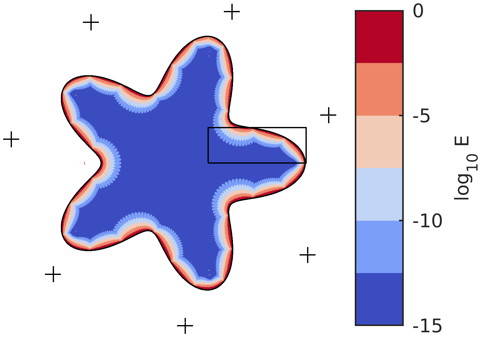
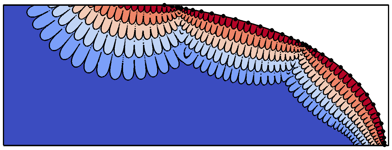
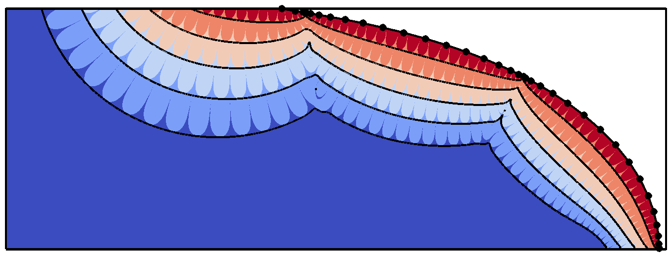
Figure 1: Figure 3 from [4]. The field shows the error when using a panel based 16-point Gauss-Legendre quadrature for evaluating the 2D Laplace double layer potential, which represents the solution to the interior boundary value problem constructed by using the field from the point sources marked with plus ($+$) signs as boundary data. The error estimates are plotted with black contours; the top right plot displays estimate (31) and the bottom right plot estimate (30).
Figure originally published in: L. af Klinteberg and A.-K. Tornberg. Adaptive Quadrature by Expansion for Layer Potential Evaluation in Two Dimensions. SIAM J. Sci. Comput., 40(3):A1225–A1249, 2018. Copyright ©2018 Society for Industrial and Applied Mathematics. Reprinted with permission. All rights reserved.

The color fields in figure 1 show the measured numerical error, and for comparison, the error estimates ($n=16$) are plotted on top with black contours in the enlarged plots for a part of the domain. To evaluate the error estimates, contributions from the two panels closest to the evaluation point have been added. The error estimates are remarkably accurate, given the simplifications that have been made. Keeping the imaginary part in the error estimate (31), we can even capture the oscillations of the error.

In figure 2, plots corresponding to the two right plots in figure 1 are shown for a discretization based on the trapezoidal rule. Here, the full curve is discretized with $n=250$ points, and the estimates used are (33) and (32).

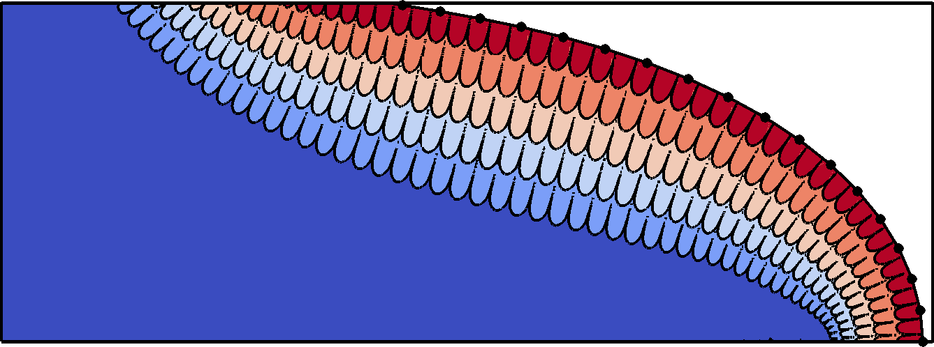
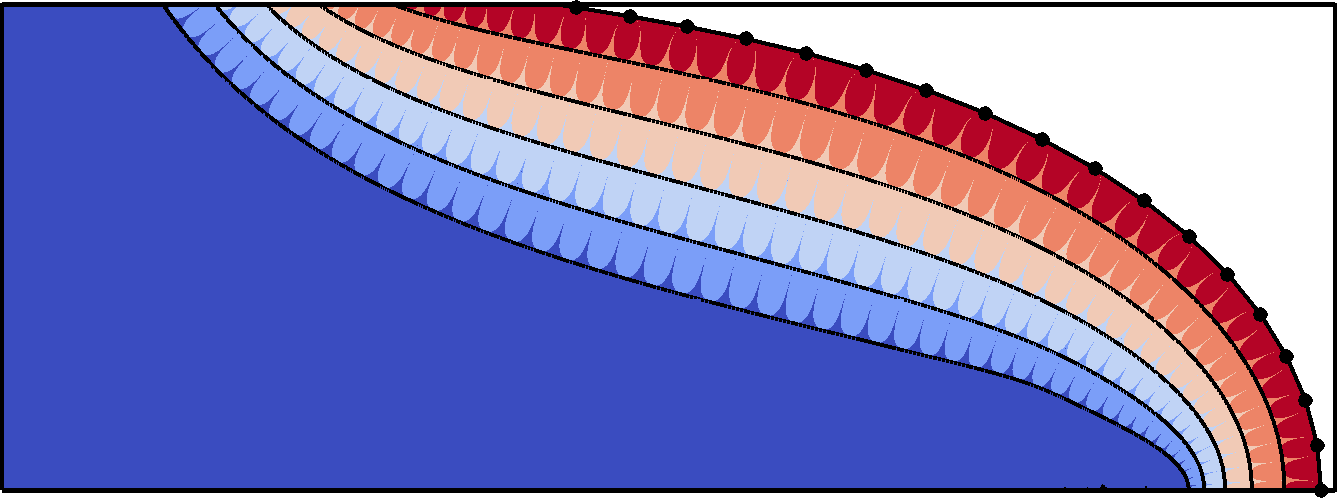
Figure 2: Plots corresponding to the two right plots in Fig. 1, but for a discretization with trapezoidal rule with $n=250$. Again, the error estimates are plotted with black contours; the left plot displays estimate (33) and the right plot estimate (32).

The error contours look different for this approximation with uniformly spaced discretizations points as compared to the panel based Gauss-Legendre discretization, but again, the precision of the estimates is excellent.

Error estimates have also been derived for the Helmholtz and Stokes equations for $n$-point Gauss-Legendre discretizations, and derivations and corresponding plots can be found in [4] and [16], respectively. Using what has been discussed above, it is straightforward to derive the corresponding results for the trapezoidal rule.

5 Quadrature errors near one-dimensional curves

In this section we will derive error estimates for the numerical evaluation of the layer potential (8). The curve $\Gamma$ can be in $\mathbb{R}^{2}$ or $\mathbb{R}^{3}$, and we will denote $\Gamma=\gamma(E)$, $E\subset\mathbb{R}$ for both cases. The form of layer potentials in $\mathbb{R}^{2}$ and $\mathbb{R}^{3}$ will be such that $p$ is a positive integer in $\mathbb{R}^{2}$ and a positive half-integer in $\mathbb{R}^{3}$. In our analysis, we will keep the two cases of $\mathbb{R}^{2}$ and $\mathbb{R}^{3}$ together, and will derive error estimates for all $p$ such that $2p\in{\mathbb{Z}}^{+}$.

As was commented on in Section 2, we will consider closed curves for the trapezoidal rule and open curves (segments) with the Gauss-Legendre quadrature rule. As introduced in section 3, the base interval $E$ is set to $[0,2\pi]$ and $[-1,1]$, respectively.

5.1 General results

We now introduce the squared distance function for a curve in $\mathbb{R}^{d}$ ($d=2$ or $3$), given an evaluation point $\bm{x}$,

$$R^{2}(t,\bm{x})\coloneqq\mathinner{\!\left\lVert\bm{\gamma}(t)-\bm{x}\right\rVert}^{2}=\sum_{i=1}^{d}(\gamma_{i}(t)-x_{i})^{2},$$ (34)

such that we can write our integral of interest (8) in the form

$$\operatorname{I}[\Theta_{p}](\bm{x})=\int_{E}\Theta_{p}(t,\bm{x})\operatorname{d\!}t,\qquad\Theta_{p}(t,\bm{x})=\frac{f(t)}{\left(R^{2}(t,\bm{x})\right)^{p}}.$$ (35)

Now, if (8) is computed using an $n$-point quadrature rule, then the error is given by the contour integral

$$\operatorname{E}_{n}[\Theta_{p}](\bm{x})=\frac{1}{2\pi i}\int_{C}\Theta_{p}(t,\bm{x})k_{n}(t)\operatorname{d\!}t=\frac{1}{2\pi i}\int_{C}\frac{f(t)k_{n}(t)\operatorname{d\!}t}{\left(R^{2}(t,\bm{x})\right)^{p}}.$$ (36)

Here, the function $k_{n}(z)$ is specific to the quadrature rule used, and was given in equations (18) and (20), respectively. $C$ is a contour containing the interval $E$, on and within which $\Theta_{p}(t,\bm{x})$ is analytic. The region of analyticity of $\Theta_{p}(t,\bm{x})$ is bounded by its singularities, which, under the assumption that $f$ is smooth, are given by the roots of the squared distance function $R^{2}$. Since $R^{2}(t,\bm{x})$ is real for real $t$, the roots will come in complex conjugate pairs. Let $\left\{t_{0},\overline{t}_{0}\right\}$ be the pair closest to $E$, such that

$$R^{2}(t_{0},\bm{x})=R^{2}(\overline{t}_{0},\bm{x})=0.$$ (37)

We will refer to these points both as roots (of $R^{2}$) and singularities (of the integrand). They are in most applications not known a priori, but can be found numerically for a given target point $\bm{x}$ (how to do this is discussed in Section 5.5).

We can deform the contour $C$ in (36) away from $E$, avoiding the singularities $t_{0}$ and $\overline{t}_{0}$, see Fig. 3. We assume that the integrand of (36) vanishes faster than $|t|^{-1}$ as $|t|\to\infty$. This means that the contributions from those parts of $C$ that are well separated from the interval $E$ will tend to zero. If we let the contour tend to infinity, deforming it to avoid also other pairs of singularities further away from $E$, the error will be given by the sum of contributions from all the singularities. Considering the fast decay of the contribution from a singularity with the distance from $E$, we further assume that we can ignore all roots to $R^{2}$ except $t_{0}$ and $\overline{t}_{0}$. For further discussion on multiple roots of $R^{2}$, see the discussion in connection to the quadrature method introduced in [2].

These assumptions let us approximate (36) using only the contributions from the pair of closest singularities, $\left\{t_{0},\overline{t}_{0}\right\}$. How these contributions are computed depends on whether or not $p$ is an integer, as we shall see in the following sections.

The following derivation will be made for a given evaluation point $\bm{x}$, and we will temporarily drop the argument $\bm{x}$ and replace $\operatorname{E}_{n}[\Theta_{p}](\bm{x})\rightarrow\operatorname{E}_{n}$ for ease of notation.

5.1.1 Integer $p$

If $p$ is integer, then $t_{0}$ and $\overline{t}_{0}$ are simply $p$th order poles. Starting from (36) and letting the contour $C$ go to infinity, we estimate the quadrature error using only the residues (as based on the assumptions made above),

$$\operatorname{E}_{n} \approx-\sum_{w=\{t_{0},\overline{t}_{0}\}}\operatorname{Res}\left[\frac{f(t)k_{n}(t)}{\left(R^{2}(t)\right)^{p}},w\right]$$ (38)

$$=-\sum_{w=\{t_{0},\overline{t}_{0}\}}\frac{1}{(p-1)!}\lim_{t\to w}\mathinner{\dfrac{\operatorname{d\!}{{}^{p-1}}}{\operatorname{d\!}{t^{p-1}}}}\left(f(t)\left(\frac{t-w}{R^{2}(t)}\right)^{p}k_{n}(t)\right).$$ (39)

Following [4], we simplify the derivative in the above expression by only keeping the term with the highest derivative of $k_{n}$. In addition, we define the geometry factor $G$, which for a root $w$ of $R^{2}$ is defined as

$$G(w)=\lim_{t\to w}\frac{t-w}{R^{2}(t)}=\left(2\left(\bm{\gamma}(w)-\bm{x}\right)\cdot\bm{\gamma}^{\prime}(w)\right)^{-1}.$$ (40)

This allows us to write

$$\operatorname{E}_{n} \approx-\frac{1}{(p-1)!}\left(f(t_{0})G(t_{0})^{p}k_{n}^{(p-1)}(t_{0})+f(\overline{t}_{0})G(\overline{t}_{0})^{p}k_{n}^{(p-1)}(\overline{t}_{0})\right)$$ (41)

$$=-\frac{2}{(p-1)!}\operatorname{Re}\left[f(t_{0})G(t_{0})^{p}k_{n}^{(p-1)}(t_{0})\right].$$ (42)

As the target point $\bm{x}$ moves parallel to the curve, this estimate oscillates in the same way as the error (see e.g. Fig. 5). Capturing these oscillations with an estimate can in some cases be hard, and is in any case of limited practical use. We therefore use the triangle inequality on (41) instead, to get a final, slightly conservative, estimate for the absolute value of the error,

$$\mathinner{\!\left\lvert\operatorname{E}_{n}\right\rvert} \approx\frac{2}{(p-1)!}\mathinner{\!\left\lvert f(t_{0})G(t_{0})^{p}k_{n}^{(p-1)}(t_{0})\right\rvert}=\frac{2}{(p-1)!}\mathinner{\!\left\lvert f(t_{0})\right\rvert}\mathinner{\!\left\lvert G(t_{0})\right\rvert}^{p}\mathinner{\!\left\lvert k_{n}^{(p-1)}(t_{0})\right\rvert}.$$ (43)

For a given quadrature rule with corresponding error function $k_{n}$, this expression is straightforward to evaluate, and we will do so in section 5.2 for the trapezoidal rule, and in section 5.3 for the Gauss-Legende rule.

As was mentioned earlier, layer potentials in the plane can be reformulated using complex variables. In Appendix B, we perform such a rewrite for the harmonic double layer potential in two dimensions, and show that the estimate in (43) matches the estimate in (27) as applied to that reformulated integral.

5.1.2 Half-integer $p$

We now consider the case when $p$ is a half-integer, $p=\bar{p}+1/2$, $\bar{p}\in\mathbb{Z}$. For this, we will be following the approach of [7].

Consider again the integral (36), with the contour $C$ depicted in Fig. 3. The integrand now has singularities of the form $(t-t_{0})^{\bar{p}+1/2}$, with branch points at the singularities. Since these singularities are not poles, we can no longer use residue calculus. Instead, we let $C_{1}$ and $C_{2}$ be the deformations of $C$ going around $t_{0}$ and $\overline{t}_{0}$ respectively, following the branch cuts going from the singularities. We now let $C$ go to infinity, and again, based on the assumptions introduced below (36), consider only the contributions from $C_{1}$ and $C_{2}$,

$$\operatorname{E}_{n}\approx\frac{1}{2\pi i}\int_{C_{1}}\frac{f(t)k_{n}(t)}{\mathinner{\!\left\lVert\bm{\gamma}(t)-\bm{x}\right\rVert}^{2p}}\operatorname{d\!}t+\frac{1}{2\pi i}\int_{C_{2}}\frac{f(t)k_{n}(t)}{\mathinner{\!\left\lVert\bm{\gamma}(t)-\bm{x}\right\rVert}^{2p}}\operatorname{d\!}t=\mathrel{\mathop{\ordinarycolon}}E_{1}+E_{2}.$$ (44)

Figure 3: The contour $C$, the deformations $C_{1}$ and $C_{2}$ going around the singularities $t_{0}$ and $\bar{t_{0}}$.

Now consider the contribution from $C_{1}$. We multiply and divide the integrand with $(t-t_{0})^{p}$ and integrate by parts $\bar{p}$ times, (ignoring endpoint contributions, since we are considering a section of a closed contour)

$$E_{1} =\frac{1}{2\pi i}\int_{C_{1}}\frac{1}{(t-t_{0})^{p}}\frac{(t-t_{0})^{p}f(t)k_{n}(t)}{\mathinner{\!\left\lVert\bm{\gamma}(t)-\bm{x}\right\rVert}^{2p}}\operatorname{d\!}t$$ (45)

$$=\frac{1}{2\pi i}\frac{1}{\prod_{q=1}^{\bar{p}}(q-p)}\int_{C_{1}}\frac{1}{\sqrt{t-t_{0}}}\mathinner{\dfrac{\operatorname{d\!}{{}^{\bar{p}}}}{\operatorname{d\!}{t^{\bar{p}}}}}\left(\frac{(t-t_{0})^{p}f(t)k_{n}(t)}{\mathinner{\!\left\lVert\bm{\gamma}(t)-\bm{x}\right\rVert}^{2p}}\right)\operatorname{d\!}t.$$ (46)

We can simplify this further using Lemma 2 in Appendix A,

$$\frac{1}{\prod_{q=1}^{\bar{p}}(q-p)}=\frac{\Gamma(1-p)}{\sqrt{\pi}}.$$ (47)

Note that the factor $(t-t_{0})^{p}f(t)/\mathinner{\!\left\lVert\bm{\gamma}(t)-\bm{x}\right\rVert}^{2p}$ is smooth on $C_{1}$, and we assume that it varies much slower than $k_{n}$. Analogous to the integer case, we first simplify by only differentiating $k_{n}$, and then we approximate the smooth part with its value at $t_{0}$ (where $k_{n}$ is largest),

$$E_{1} \approx\frac{1}{2\pi i}\frac{\Gamma(1-p)}{\sqrt{\pi}}G(t_{0})^{p}f(t_{0})\int_{C_{1}}\frac{k_{n}^{(\bar{p})}(t)}{\sqrt{t-t_{0}}}\operatorname{d\!}t.$$ (48)

Denote the sides of $C_{1}$ by $C_{1}^{+}$ (going out) and $C_{1}^{-}$ (going in). Defining the jump across the branch cut as

$$(t-t_{0})\Big{|}_{C_{1}^{+}}=(t-t_{0})\Big{|}_{C_{1}^{-}}e^{-2\pi i},$$ (49)

we have that

$$(t-t_{0})^{-1/2}\Big{|}_{C_{1}^{+}}=-(t-t_{0})^{-1/2}\Big{|}_{C_{1}^{-}},$$ (50)

which lets us write the $C_{1}$ contribution as

$$\int_{C_{1}}\frac{k_{n}^{(\bar{p})}(t)}{\sqrt{t-t_{0}}}\operatorname{d\!}t =\int_{t_{0}}^{\infty}\frac{k_{n}^{(\bar{p})}(t)}{\sqrt{t-t_{0}}\Big{|}_{C_{1}^{+}}}\operatorname{d\!}t+\int_{\infty}^{t_{0}}\frac{k_{n}^{(\bar{p})}(t)}{\sqrt{t-t_{0}}\Big{|}_{C_{1}^{-}}}\operatorname{d\!}t=-2\int_{t_{0}}^{\infty}\frac{k_{n}^{(\bar{p})}(t)}{\sqrt{t-t_{0}}}\operatorname{d\!}t.$$ (51)

Going back to using $p$ rather than $\bar{p}$, we define

$$J(t_{0},n,p)=\int_{t_{0}}^{\infty}\frac{k_{n}^{(p-1/2)}(t)}{\sqrt{t-t_{0}}}\operatorname{d\!}t,$$ (52)

where the integration from $t_{0}$ to $\infty$ is to follow the branch cut. With this, we get

$$E_{1} \approx\frac{\Gamma(1-p)}{i\pi^{3/2}}G(t_{0})^{p}f(t_{0})J(t_{0},n,p).$$ (53)

Repeating the calculations for $C_{2}$ with the pole at $\bar{t}_{0}$, we find $E_{2}=\bar{E}_{1}$. Similar to the previous section, we use the triangle inequality when adding up $E_{1}$ and $E_{2}$ to get a slightly conservative estimate. In addition, we simplify using the relation $\mathinner{\!\left\lvert\Gamma(1-p)\right\rvert}=\pi/\Gamma(p)$, which is a special case of Euler’s reflection formula for $p$ half-integer. Our final form for the absolute value of the error is then

$$\mathinner{\!\left\lvert\operatorname{E}_{n}\right\rvert}\approx\frac{2}{\Gamma(p)\sqrt{\pi}}\mathinner{\!\left\lvert J(t_{0},n,p)G(t_{0})^{p}f(t_{0})\right\rvert}=\frac{2}{\Gamma(p)\sqrt{\pi}}\mathinner{\!\left\lvert J(t_{0},n,p)\right\rvert}\mathinner{\!\left\lvert G(t_{0})\right\rvert}^{p}\mathinner{\!\left\lvert f(t_{0})\right\rvert}.$$ (54)

In order for this expression to be useful, a closed-form estimate for $J(t_{0},n,p)$ is needed. Such an estimate can be derived by defining a suitable branch cut with respect to the error function $k_{n}$, as we shall see in the cases of the trapezoidal and Gauss-Legendre quadrature rules.

5.2 Trapezoidal rule

For the trapezoidal rule, we are considering the integral in (35), with the integration interval $E=[0,2\pi)$ and an integrand that is assumed to be periodic in $t$. The corresponding error function is given in (20), with an asymptotic form for $n\to\infty$ in (22). The derivatives of this function is given in (23) with a somewhat simpler expression for the magnitude in (24).

5.2.1 Trapezoidal rule with integer $p$

For the trapezoidal rule with integer $p$, formulating an error estimate is just a matter of combining (43) and (24), giving Error estimate 3.

Error estimate 3 (Trapezoidal rule with integer $p$).

Consider the integral in (35), where $\gamma(E)$ is the parameterization of a smooth closed curve in $\mathbb{R}^{2}$ or $\mathbb{R}^{3}$. The integrand is assumed to be periodic in $t$ over the integration interval $E=[0,2\pi)$. The error in approximating the integral with the $n$-point trapezoidal rule can in the limit $n\rightarrow\infty$ be estimated as

$$\mathinner{\!\left\lvert\operatorname{E}_{n}[\Theta_{p}](\bm{x})\right\rvert}\approx\frac{4\pi n^{p-1}}{(p-1)!}\mathinner{\!\left\lvert f(t_{0})\right\rvert}\mathinner{\!\left\lvert G(t_{0})\right\rvert}^{p}e^{-n|\operatorname{Im}t_{0}|}.$$ (55)

Here, $p$ is a positive integer, and the geometry factor $G$ is defined in (40). The squared distance function is defined in (34), and $\left\{t_{0},\overline{t}_{0}\right\}$ is the pair of complex conjugate roots of this $R^{2}(t,\bm{x})$ closest to the integration interval $E$.

5.2.2 Trapezoidal rule with half-integer $p$

For the trapezoidal rule with half-integer $p$, we must derive an expression for $J(t_{0},n,p)$, as defined in (52), with derivatives of $k_{n}$ as given in (23). We can without loss of generality assume that $\operatorname{Im}t_{0}>0$. Let the branch cut going from $t_{0}$ to infinity be

$$B(t_{0})=\{t(s)\in\mathbb{C}\mathrel{\mathop{\ordinarycolon}}t(s)=t_{0}+is,\ \ 0\leq s<\infty\},$$ (56)

and let this be the branch cut enclosed by the path $C_{1}$ in (46). Note that along this cut

$$t^{\prime}(s) =i,$$ (57)

$$t(s)-t_{0} =is,$$ (58)

such that

$$J(t_{0},n,p)=\sqrt{i}\int_{0}^{\infty}\frac{k_{n}^{(p-1/2)}(t_{0}+is)}{\sqrt{s}}\operatorname{d\!}s\approx-2\pi i\sqrt{i}(in)^{p-1/2}e^{int_{0}}\underbrace{\int_{0}^{\infty}\frac{e^{is}}{\sqrt{s}}\operatorname{d\!}s}_{\sqrt{\pi/n}}.$$ (59)

Considering only the absolute value,

$$\mathinner{\!\left\lvert J(z_{0},n,p)\right\rvert}\approx 2\pi^{3/2}n^{p-1}e^{-n|\operatorname{Im}t_{0}|},$$ (60)

finally yields Error estimate 4.

Error estimate 4 (Trapezoidal rule with half-integer $p$).

Consider the integral in (35), where $\gamma(E)$ is the parameterization of a smooth closed curve in $\mathbb{R}^{2}$ or $\mathbb{R}^{3}$. The integrand is assumed to be periodic in $t$ over the integration interval $E=[0,2\pi)$. The error in approximating the integral with the $n$-point trapezoidal rule can in the limit $n\rightarrow\infty$ be estimated as

$$\mathinner{\!\left\lvert\operatorname{E}_{n}[\Theta_{p}](\bm{x})\right\rvert}\approx\frac{4\pi n^{p-1}}{\Gamma(p)}\mathinner{\!\left\lvert f(t_{0})\right\rvert}\mathinner{\!\left\lvert G(t_{0})\right\rvert}^{p}e^{-n|\operatorname{Im}t_{0}|}.$$ (61)

Here, $p$ is a positive half-integer, $\Gamma(p)$ the gamma function, and the geometry factor $G$ is defined in (40). The squared distance function is defined in (34), and $\left\{t_{0},\overline{t}_{0}\right\}$ is the pair of complex conjugate roots of this $R^{2}(t,\bm{x})$ closest to the integration interval $E$.

Interestingly, this is identical to the estimate (55) for integer $p$, if we generalize the factorial to non-integer $p$ as $(p-1)!=\Gamma(p)$. This generalization can be found in [3] for both the trapezoidal and Gauss-Legendre rules, where it was noted that it works well for half-integer $p$. What we have shown here (and will show in Section 5.3.2) is why it works well.

5.3 Gauss-Legendre rule

For the Gauss-Legendre quadrature rule we consider the integral in (35) over the base interval $E=[-1,1]$. The error function is not available in closed form, but can in the limit $n\to\infty$ be shown to asymptotically satisfy the formula (18) [7], here written as

$$k_{n}(z)\simeq\frac{2\pi}{\xi(z)^{2n+1}},$$ (62)

where

$$\xi(z)=z+\sqrt{z^{2}-1}.$$ (63)

As was introduced below equation (18), $\sqrt{z^{2}-1}$ is defined as $\sqrt{z+1}\sqrt{z-1}$ with $-\pi<\arg(z\pm 1)\leq\pi$ [7]. Alternatively, we can write $\xi(z)=z\pm\sqrt{z^{2}-1}$, with the sign defined such that $|\xi|\geq 1$. The approximation of the derivatives of $k_{n}(z)$ as introduced in (21) will include the same factor of $1/\xi(z)^{2n+1}$.

The main characteristic of the asymptotic Gauss-Legendre error function (62) is that its magnitude is constant on the level sets of the function

$$\rho(z)=\mathinner{\!\left\lvert\xi(z)\right\rvert},$$ (64)

which we denote the Bernstein radius of $z$. This follows from the notion of a Bernstein ellipse, which is an ellipse with foci $\pm 1$ where the semimajor and semiminor axes sum to $\rho>1$. It can be constructed as the image of the circle $|\xi|=\rho$ under the Joukowski transform

$$z(\xi)=\frac{\xi+\xi^{-1}}{2},$$ (65)

which is the inverse of (63).

5.3.1 Gauss-Legendre rule with integer $p$

For the Gauss-Legendre rule with integer $p$, we can combine (43) and (21) to get the following error estimate.

Error estimate 5 (Gauss-Legendre rule with integer $p$).

Consider the integral in (35) , where $\gamma(E)$ is the parameterization of a smooth curve in $\mathbb{R}^{2}$ or $\mathbb{R}^{3}$, with $E=[-1,1]$. The error in approximating the integral with the $n$-point Gauss-Legendre rule can in the limit $n\rightarrow\infty$ be estimated as

$$\mathinner{\!\left\lvert\operatorname{E}_{n}[\Theta_{p}](\bm{x})\right\rvert}\approx\frac{4\pi}{(p-1)!}\mathinner{\!\left\lvert\frac{2n+1}{\sqrt{t_{0}^{2}-1}}\right\rvert}^{p-1}\mathinner{\!\left\lvert f(t_{0})\right\rvert}\mathinner{\!\left\lvert G(t_{0})\right\rvert}^{p}\frac{1}{\rho(t_{0})^{2n+1}}.$$ (66)

Here, $p$ is a positive integer, the geometry factor $G$ is defined in (40) and $\rho(t)=|t+\sqrt{t+1}\sqrt{t-1}|$. The squared distance function is defined in (34), and $\left\{t_{0},\overline{t}_{0}\right\}$ is the pair of complex conjugate roots of this $R^{2}(t,\bm{x})$ closest to the integration interval $E$.

5.3.2 Gauss-Legendre rule with half-integer $p$

In order to evaluate the integral (52) with the Gauss-Legendre error function (21), we will closely follow the steps outlined by Elliott et al. [7]. We define a branch cut going from $t_{0}$ to infinity (again, assuming without loss of generality that $\operatorname{Im}t_{0}>0$) using a scaled Joukowsky transform,

$$B(t_{0})=\left\{t(s)\in\mathbb{C}\mathrel{\mathop{\ordinarycolon}}t(s)=\frac{1}{2}\left(\zeta(s)+\frac{1}{\zeta(s)}\right),\ \ 1\leq s<\infty\right\},$$ (67)

where $\zeta(s)$ parameterizes a radial line from the point $\zeta_{0}=t_{0}+\sqrt{t_{0}^{2}-1}$ to infinity,

$$\zeta(s)=\zeta_{0}s$$ (68)

and $\rho(t_{0})=|\zeta_{0}|$ as introduced above. This parametrization of the branch cut satisfies $t(1)=t_{0}$, and leads to the following useful relations,

$$t^{\prime}(s) =\frac{\zeta_{0}}{2}\left(1-\frac{1}{\zeta_{0}^{2}s^{2}}\right),$$ (69)

$$t(s)-t_{0} =\frac{\zeta_{0}(s-1)}{2}\left(1-\frac{1}{\zeta_{0}^{2}s}\right),$$ (70)

$$\sqrt{t(s)^{2}-1} =\frac{\zeta(s)}{2}\left(1-\frac{1}{\zeta(s)^{2}}\right)=st^{\prime}(s).$$ (71)

Together with the relation $\xi(t(s))=\zeta(s)$, this lets us write (21) as

$$k_{n}^{(\bar{p})}(t(s))\approx\left(-\frac{2n+1}{st^{\prime}(s)}\right)^{\bar{p}}\frac{2\pi}{\zeta(s)^{2n+1}}.$$ (73)

With substitution of the above relations, reverting to use only $p=\bar{p}+1/2$ we can write (52) as

$$\begin{split}&J(t_{0},n,p)=\int_{1}^{\infty}\frac{k_{n}^{(p-1/2)}(t(s))}{\sqrt{t(s)-t_{0}}}t^{\prime}(s)\operatorname{d\!}s\\ &\approx\left(-(4n+2)\right)^{p-1/2}\frac{\pi\sqrt{2}}{\zeta_{0}^{2n+p}}\int_{1}^{\infty}\frac{1}{s^{2n+p+\frac{1}{2}}\sqrt{s-1}}\frac{1}{\sqrt{1-\frac{1}{\zeta_{0}^{2}s}}}\left(1-\frac{1}{\zeta_{0}^{2}s^{2}}\right)^{3/2-p}\operatorname{d\!}s.\end{split}$$ (74)

By assuming that most of the contribution to the integral comes from the neighborhood of $s=1$, we make the simplifications

$$1-\frac{1}{\zeta_{0}^{2}s^{2}}\approx 1-\frac{1}{\zeta_{0}^{2}s}\approx 1-\frac{1}{\zeta_{0}^{2}}=\frac{2}{\zeta_{0}}\sqrt{t_{0}^{2}-1}.$$ (75)

Then,

$$J(t_{0},n,p)\approx\frac{2\pi i\sqrt{(2n+1)}}{\zeta_{0}^{2n+1}}\left(-\frac{2n+1}{\sqrt{t_{0}^{2}-1}}\right)^{p-1}\int_{1}^{\infty}\frac{1}{s^{2n+p+\frac{1}{2}}\sqrt{s-1}}\operatorname{d\!}s.$$ (76)

This can be simplified using the result from [7] that for $N$ large,

$$\int_{1}^{\infty}\frac{\operatorname{d\!}s}{s^{N}\sqrt{s-1}}\approx\sqrt{\frac{\pi}{N}},$$ (77)

such that, taking the absolute value and reintroducing $|\zeta_{0}|=\rho(t_{0})$ we get

$$\mathinner{\!\left\lvert J(t_{0},n,p)\right\rvert}\approx\pi^{3/2}\sqrt{\frac{4(2n+1)}{2n+p+1/2}}\mathinner{\!\left\lvert\frac{2n+1}{\sqrt{t_{0}^{2}-1}}\right\rvert}^{p-1}\frac{1}{\rho(t_{0})^{2n+1}}.$$ (78)

Assuming $n$ large and $p\geq 1/2$ of moderate values, we approximate $(2n+1)/(2n+1/2+p)\approx 1$, such that

$$\mathinner{\!\left\lvert J(t_{0},n,p)\right\rvert}\approx 2\pi^{3/2}\mathinner{\!\left\lvert\frac{2n+1}{\sqrt{t_{0}^{2}-1}}\right\rvert}^{p-1}\frac{1}{\rho(t_{0})^{2n+1}}.$$ (79)

Inserting this into (54), we get

Error estimate 6 (Gauss-Legendre rule with half-integer $p$).

Consider the integral in (35) , where $\gamma(E)$ is the parameterization of a smooth curve in $\mathbb{R}^{2}$ or $\mathbb{R}^{3}$, with $E=[-1,1]$. The error in approximating the integral with the $n$-point Gauss-Legendre rule can in the limit $n\rightarrow\infty$ be estimated as

$$\mathinner{\!\left\lvert\operatorname{E}_{n}[\Theta_{p}](\bm{x})\right\rvert}\approx\frac{4\pi}{\Gamma(p)}\mathinner{\!\left\lvert\frac{2n+1}{\sqrt{t_{0}^{2}-1}}\right\rvert}^{p-1}\mathinner{\!\left\lvert f(t_{0})\right\rvert}\mathinner{\!\left\lvert G(t_{0})\right\rvert}^{p}\frac{1}{\rho(t_{0})^{2n+1}}.$$ (80)

Here, $p$ is a positive half-integer, $\Gamma(p)$ the gamma function, the geometry factor $G$ is defined in (40) and $\rho(t)=|t+\sqrt{t+1}\sqrt{t-1}|$. The squared distance function is defined in (34), and $\left\{t_{0},\overline{t}_{0}\right\}$ is the pair of complex conjugate roots of this $R^{2}(t,\bm{x})$ closest to the integration interval $E$.

Analogously to the trapezoidal rule case, this estimate is identical to the estimate (66) for integer $p$, with the generalization $(p-1)!=\Gamma(p)$.

5.4 Examples for one-dimensional curves in $\mathbb{R}^{2}$

The estimates in Sections 5.2 and 5.3 for the nearly singular quadrature error are derived using a number of simplifications, in order to get closed-form expressions without any unknown constants. Nevertheless, they have excellent predictive accuracy. To demonstrate this, we consider the simple layer potential

$$u(\bm{x})=\int_{0}^{2\pi}\frac{\mathinner{\!\left\lVert\bm{\gamma}^{\prime}(t)\right\rVert}\operatorname{d\!}t}{\mathinner{\!\left\lVert\bm{\gamma}(t)-\bm{x}\right\rVert}^{2p}},$$ (81)

for $p=\frac{1}{2},1,\frac{3}{2},2$ and points $\bm{x}$ near the planar curve defined by

$$\bm{\gamma}(t)=\left(1+0.1\cos(5t)\right)\begin{pmatrix}\cos(t)\\ \sin(t)\end{pmatrix},\quad t\in[0,2\pi).$$ (82)

We discretize the integration interval $[0,2\pi)$ in two ways: using the composite Gauss-Legendre method with 20 equisized panels and $n$ points per panel, and using the global trapezoidal rule with $n$ points along the curve. This gives us the quadrature value $\operatorname{Q}_{n}$ for each $\bm{x}$. We compute the reference value using an adaptive quadrature routine (Matlab’s integral with AbsTol=0 and RelTol=0). Then we can compute an accurate value of $\operatorname{E}_{n}$, which we compare to Error estimates 3, 4, 5 and 6. Note that in the case of composite Gauss-Legendre, $\operatorname{E}_{n}$ is calculated as the sum of the contributions from the 3 panels nearest to $\bm{x}$.

5.4.1 Error contours

In order to compare our estimates to the actual quadrature error, we need target points $\bm{x}$ for which the corresponding root $t_{0}$ is known. Before entering the discussion of how to compute $t_{0}$, we will demonstrate our estimates for target points $\bm{x}$ for which $t_{0}$ is analytically known. We define such points through complexification of the curve parametrization, such that they by construction are roots to the squared distance function (34). That is, we first set $t_{0}\in\mathbb{C}$, and then construct the corresponding $\bm{x}$ as

$$\bm{x}(t_{0})=\begin{pmatrix}\operatorname{Re}\omega(t_{0})\\ \operatorname{Im}\omega(t_{0})\end{pmatrix}\quad\mbox{ where }\quad\omega(t)=\gamma_{1}(t)+i\gamma_{2}(t).$$ (83)

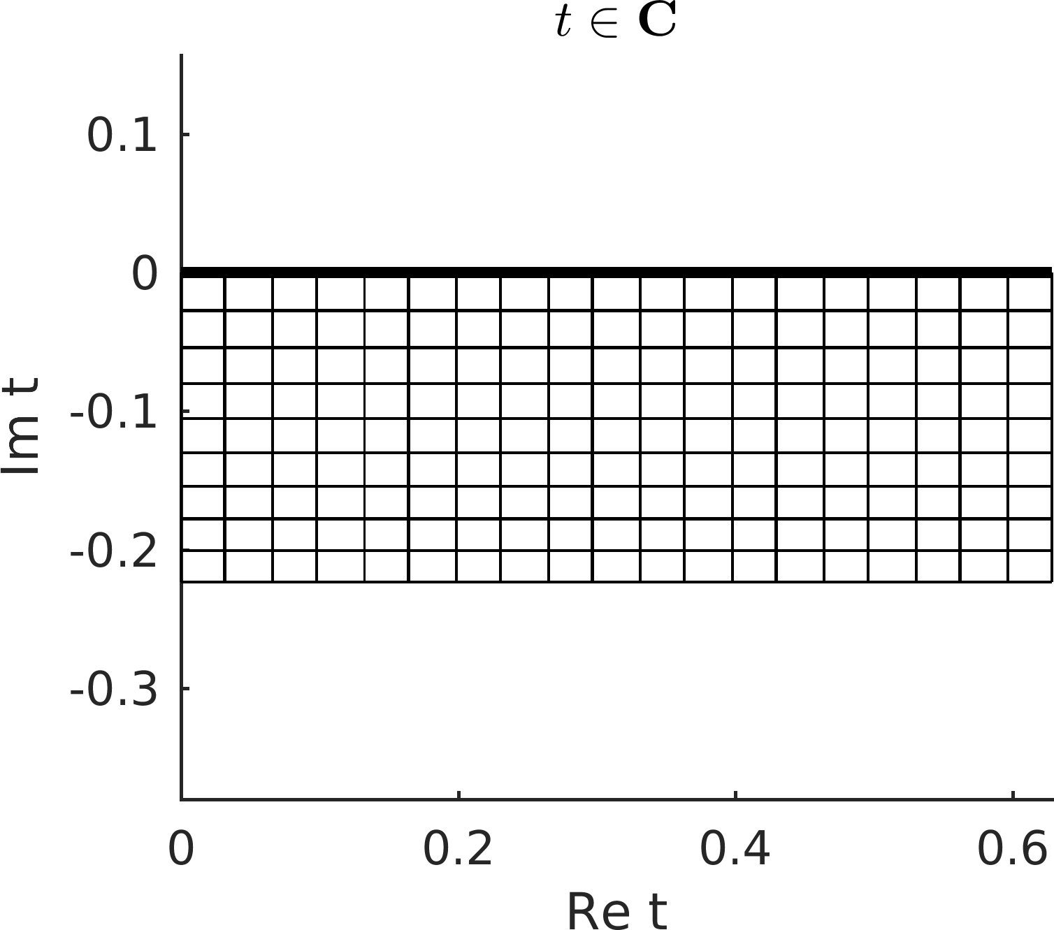
(a) Grid in complex parametrization space.

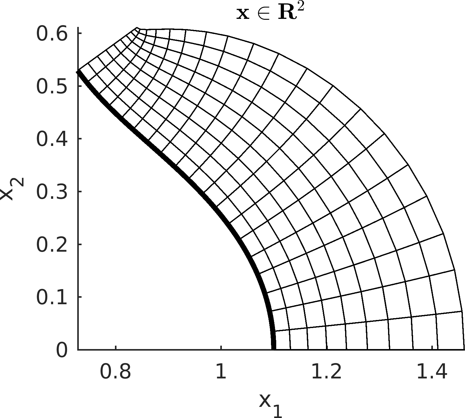
(b) Image of grid in physical space.

Figure 4: Correspondence between complex points near the real axis (thick line), and points near a segment of the curve parametrized by (82), under the complexification (83).

This mapping is illustrated in Fig. 4. We construct a grid of $200\times 100$ points covering the region shown in that figure, and consider the evaluation of the integral (81) at those target points, for $p=3/2$. We compute the integral with Gauss-Legendre and 20 panels with 16 points each, and with the trapezoidal rule and 200 points on the entire curve. Then we estimate the quadrature error using (61) and (80). Comparing the level contours of the errors and the estimates, see Fig. 5(a), it is clear that they match well. The estimate is a smooth envelope of the node-frequency oscillations in the quadrature error, and therefore provides an estimated upper bound of the error. The enveloping is due to our use of the triangle inequality when combining the errors from the two singularities. A more precise estimate that includes the node frequency oscillations can be obtained by skipping this step, compare e.g. section 4.1, but it does risk underestimating the error at some points if the oscillations do not match perfectly.

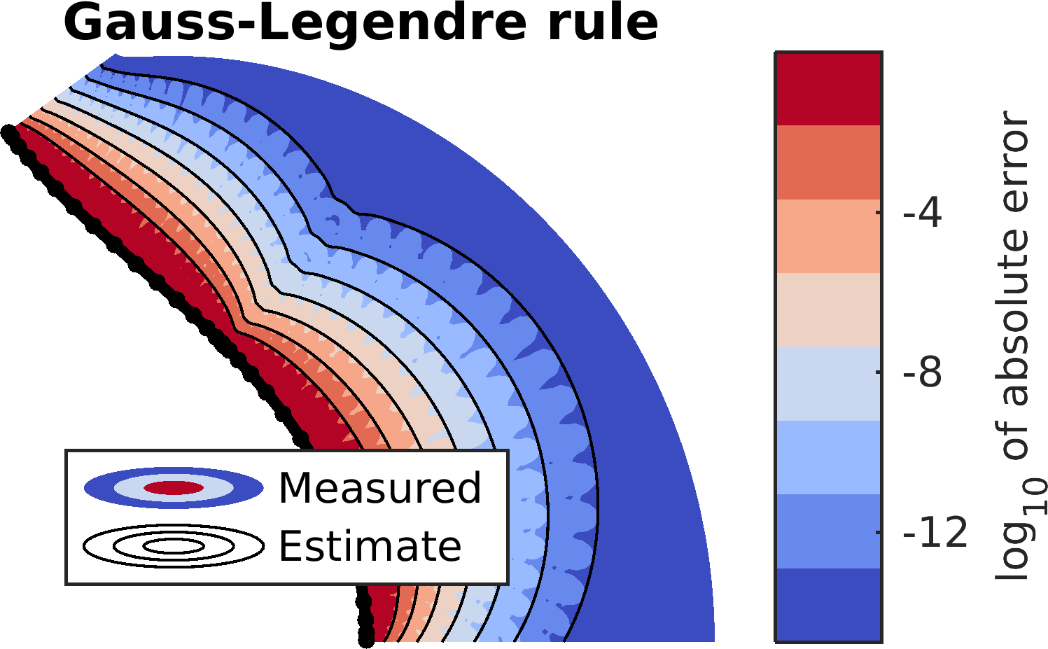
(a) GL, 20 panels, $n=16$

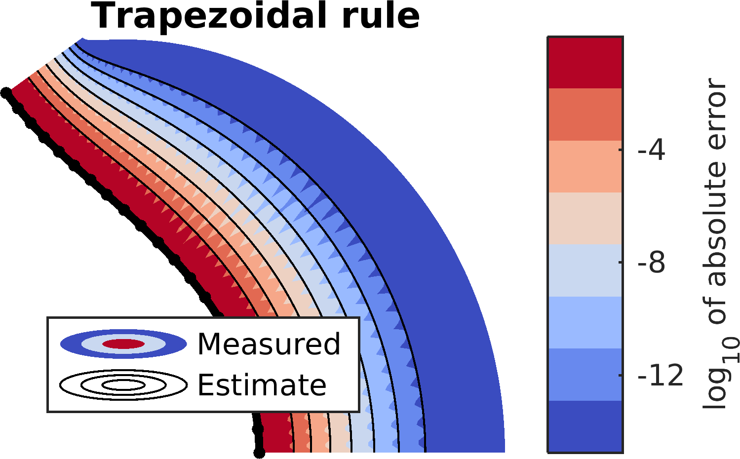
(b) Trapezoidal, $n=200$

Figure 5: Quadrature error vs estimate for $p=3/2$.

5.4.2 Convergence of errors and precision of error estimates

In Fig. 5 we see that the the error estimates can match the errors well in space, for a given value of $n$ and $p$. In an attempt to show how the error varies and how well this is captured by our estimates, we now study the convergence with respect to $n$ for a number of values of $p$. For this, we first attempt to construct a large number of random points for which the magnitude of the error is of the same magnitude, i.e. points that lie along one of the contours in Fig. 5. In the case of the trapezoidal rule, this is straightforward: we simply generate random points with $|\operatorname{Im}t_{0}|$ fixed and $\operatorname{Re}t_{0}\in[0,2\pi)$. For the Gauss-Legendre rule, we need points such that $\rho(t_{0})$ has a fixed value in the parametrization of the panel closest to the points. We create them for each panel by applying the Joukowski transform (65) to random points on a semicircle of radius $\rho$, and then keeping the points such that $-1<\operatorname{Re}t_{0}<1$. In both cases, we determine $\bm{x}$ from $t_{0}$ using the complexification (83). Figure 6 shows our test points generated in this way.

Consider the results in Fig. 7. The plots to the right show the errors as the sets of target points in Fig. 6 are traversed, for a number of $p$ and fixed $n$. The estimates clearly provide a good approximate upper bound of the error. The plots to the left shows how the maximum error over all the target points converges towards zero as $n$ increases, for a number of $p$. That value is compared to the estimate, which is computed at the point with the maximum error. We see that the estimates capture both the magnitude of of the errors and the rates of convergence as $n$ increases.

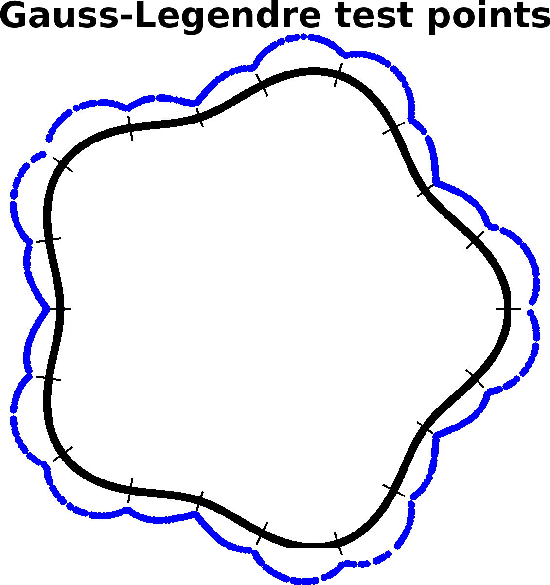
(a) Target points with $\rho(t_{0})=1.05$ in the parametrization of the nearest panel.

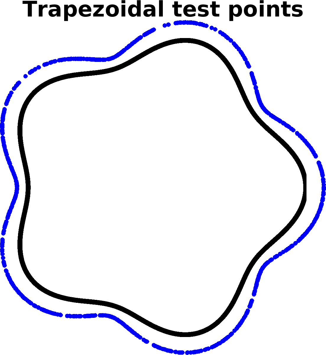
(b) Target points with $|\operatorname{Im}t_{0}|=0.1$.

Figure 6: Source geometry (black) and test points (blue) used when evaluating quadrature errors and error estimates for the Gauss-Legendre and trapezoidal rules, respectively. In each case the number of test points is 1000. For the Gauss-Legendre case, the subdivision into 20 panels is also shown.

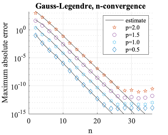
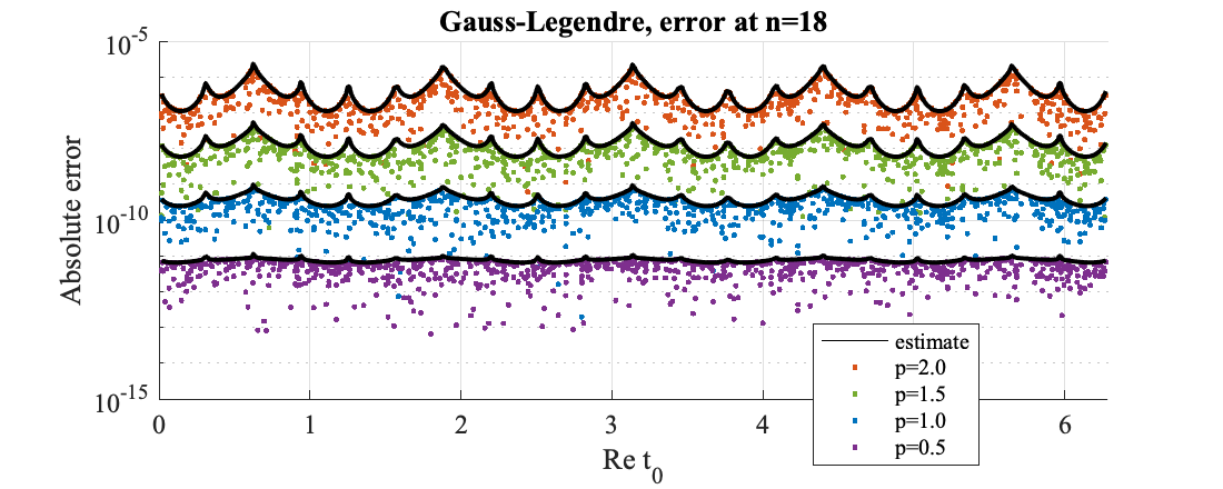
(a) Gauss-Legendre convergence

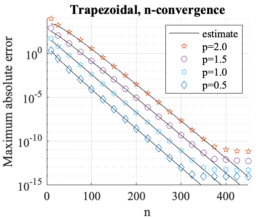
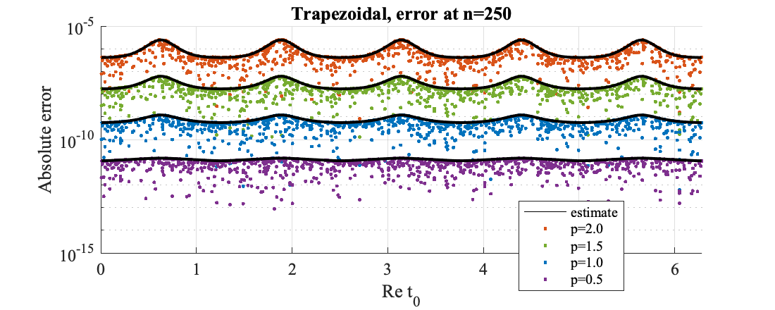
(b) Trapezoidal convergence

Figure 7: Errors in approximation the layer potential in (81) by the (a) Gauss-Legendre rule applied to each of $20$ panels, and (b) the trapezoidal rule. The errors are measured at the points shown in Fig. 6$a)$ and Fig. 6$b)$, respectively. For the $n$-convergence we report the value of the estimate at the point with the largest error.

5.5 Root finding

As we have seen, we can accurately predict the magnitudes of the nearly singular quadrature errors for one-dimensional curves discretized using the trapezoidal and Gauss-Legendre rules. However, in order to do so for given target point $\bm{x}$, we need to know the location of the nearest complex root $t_{0}$ of the squared distance function (34). Fortunately, finding $t_{0}$ numerically is both fast and robust, using only the discrete quadrature nodes on the curve. A method for the Gauss-Legendre case was introduced in [4] for curves in $\mathbb{R}^{2}$, and further developed in [2] for curves in both $\mathbb{R}^{2}$ and $\mathbb{R}^{3}$. We will here summarize these results, generalize them for the trapezoidal rule, and then introduce simplifications that will prove useful in the three-dimensional case.

In order to determine $t_{0}$ without explicit knowledge of the parametrization $\bm{\gamma}(t)$, we form an approximation to it, denoted $\tilde{\bm{\gamma}}(t)$. The most straightforward way of doing this, and also the most accurate and expensive way, is to use the values at the $n$ quadrature nodes $t_{\ell}$, $\ell=1,\dots,n$. For a Gauss-Legendre panel $t_{\ell}\in[-1,1]$, for the trapezoidal rule $t_{\ell}\in[0,2\pi)$. Then, an interpolant is created for each of the $d$ components of $\bm{\gamma}\in\mathbb{R}^{d}$ using suitable orthogonal basis functions. For Gauss-Legendre we use a basis $\{P_{j}\}$ of orthogonal polynomials on $[-1,1]$ (e.g. Chebyshev or Legendre),

$$\tilde{\gamma}_{i}(t)=\operatorname{P}_{n}[\gamma_{i}](t)=\sum_{j=0}^{n-1}c_{j}P_{j}(t),\quad i=1,\ldots,d,$$ (84)

while for trapezoidal we use a trigonometric polynomial,

$$\tilde{\gamma}_{i}(t)=\operatorname{F}_{n}[\gamma_{i}](t)=\sum_{k=-n/2}^{n/2-1}\hat{\gamma}_{i}(k)e^{ikt},\quad i=1,\ldots,d.$$ (85)

Once we have $\tilde{\bm{\gamma}}$, we can form an approximation to the squared distance function in (34),

$$\tilde{R}^{2}(t)=\sum_{i=1}^{d}(\tilde{\gamma}_{i}(t)-x_{i})^{2}=0.$$ (86)

The roots to this equation can be found to high accuracy using Newton’s method and a suitable initial guess, see discussion in [2]. The method typically converges rapidly, and has a cost of $\mathcal{O}(n)$ per iteration, for the evaluation of $\tilde{\bm{\gamma}}$. This is related to the procedure introduced in [4] for complex kernels as described in section 4. There, we create a complex-valued approximation $\tilde{\gamma}(t)\approx\gamma(t)$, and given $z_{0}$ we solve $\tilde{\gamma}(t_{0})=z_{0}$ for the pre-image $t_{0}$. This procedure can however not be generalized to three dimensions. For a planar curve, the pre-image corresponds to one of the two roots of $\tilde{R}^{2}(t)$.

As described, this is a reasonably efficient scheme for a Gauss-Legendre panel, where $n$ rarely is more than $16$, but cannot be considered efficient for the trapezoidal rule, where $n$ is the number of points on the entire curve. This is especially true since estimating the quadrature error is not in itself a necessary computation, and should not incur a significant extra cost. However, we only need to know $t_{0}$ with sufficient accuracy to estimate the quadrature error to the correct order of magnitude. Thus, we can consider ways of computing $t_{0}$ that are faster, but less accurate.

Let $\tilde{\bm{\gamma}}$ approximated using (84) or (85) be denoted the global approximation (with respect to the quadrature rule). Note however that it is only for the trapezoidal rule that it is truly global, for Gauss-Legendre it involves one full panel. Then, we denote the local approximation to be the $q$th order Taylor expansion

$$\tilde{\gamma}_{i}(t)=\operatorname{T}_{q}[\gamma_{i},t^{*}](t)=\sum_{j=0}^{q}\gamma_{i}^{(j)}(t^{*})\frac{\left(t-t^{*}\right)^{j}}{j!},$$ (87)

where $t^{*}$ is the value of the parametrization at the quadrature node that is closest to $\bm{x}$,

$$t^{*}=\operatornamewithlimits{argmin}_{t\in\{t_{1},\dots,t_{n}\}}\mathinner{\!\left\lVert\bm{\gamma}(t)-\bm{x}\right\rVert}$$ (88)

and can be identified using e.g. a tree-based search algorithm.

Solving (86) using Newton’s method, with the approximation (87) and a moderate value of $q$, allows us to compute $t_{0}$ rapidly and with sufficient accuracy for error estimation (as we shall demonstrate). The prerequisite is that we need to know all derivatives of $\bm{\gamma}$ up to $\bm{\gamma}^{(q)}(t)$ at all quadrature nodes, which may not be available. These can however be computed numerically at the time of discretization, which is a one-time cost (as opposed to finding $t_{0}$ for all target points $\bm{x}$, which we consider an on-the-fly cost). The resulting root finding scheme is of course independent of the quadrature, but is most useful for the trapezoidal rule where the alternative of global approximation really involves the discretization of the whole curve.

Figure 8 revisits our trapezoidal rule example from Section 5.4.1. This time, instead of using the known roots to evaluate the estimates, we use roots that are computed with the combination of Newton’s method and Taylor expansion, for a few different orders $q$. Essentially, what we are are doing is computing the inverse of the complexification $\omega(t)$ in (83). Not surprisingly, low order approximations introduce a distortion in this map, that increases with local curvature and distance from the curve. However, with only moderate values of $q$ it is possible to compute the root sufficiently well for the contours of the estimate to follow the error contours closely, at least in this particular example.

(a) Inverse of $\operatorname{T}_{1}[\bm{\gamma}]$.

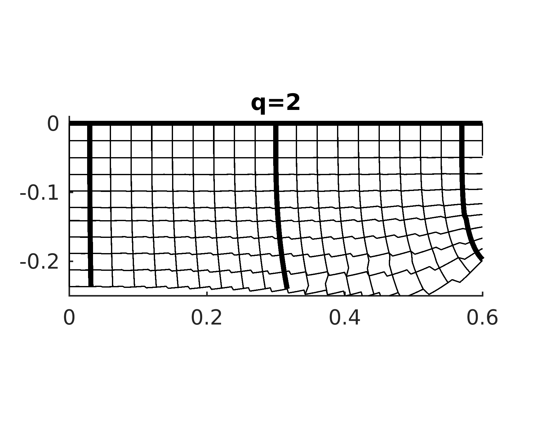
(b) Inverse of $\operatorname{T}_{2}[\bm{\gamma}]$.

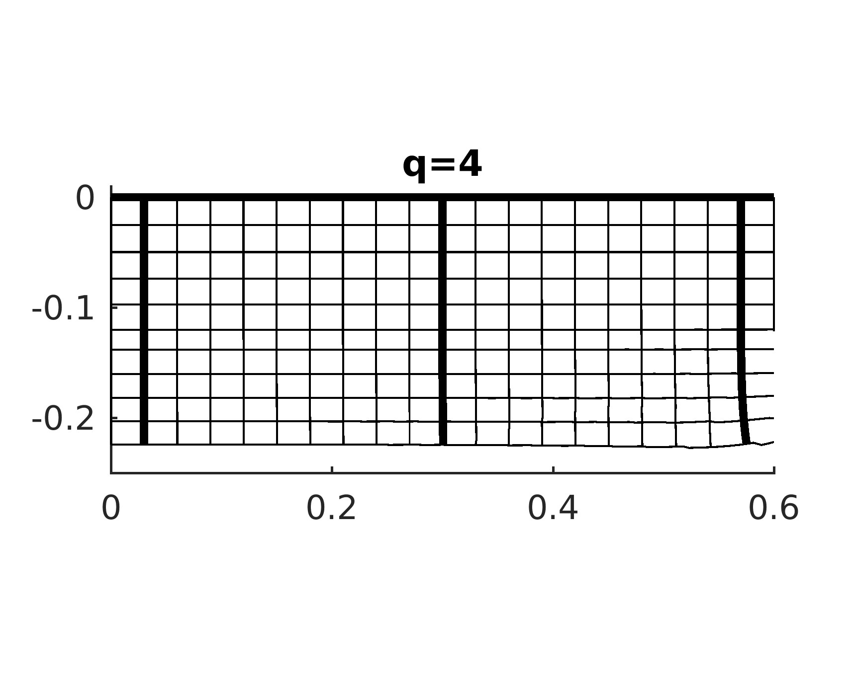
(c) Inverse of $\operatorname{T}_{4}[\bm{\gamma}]$.

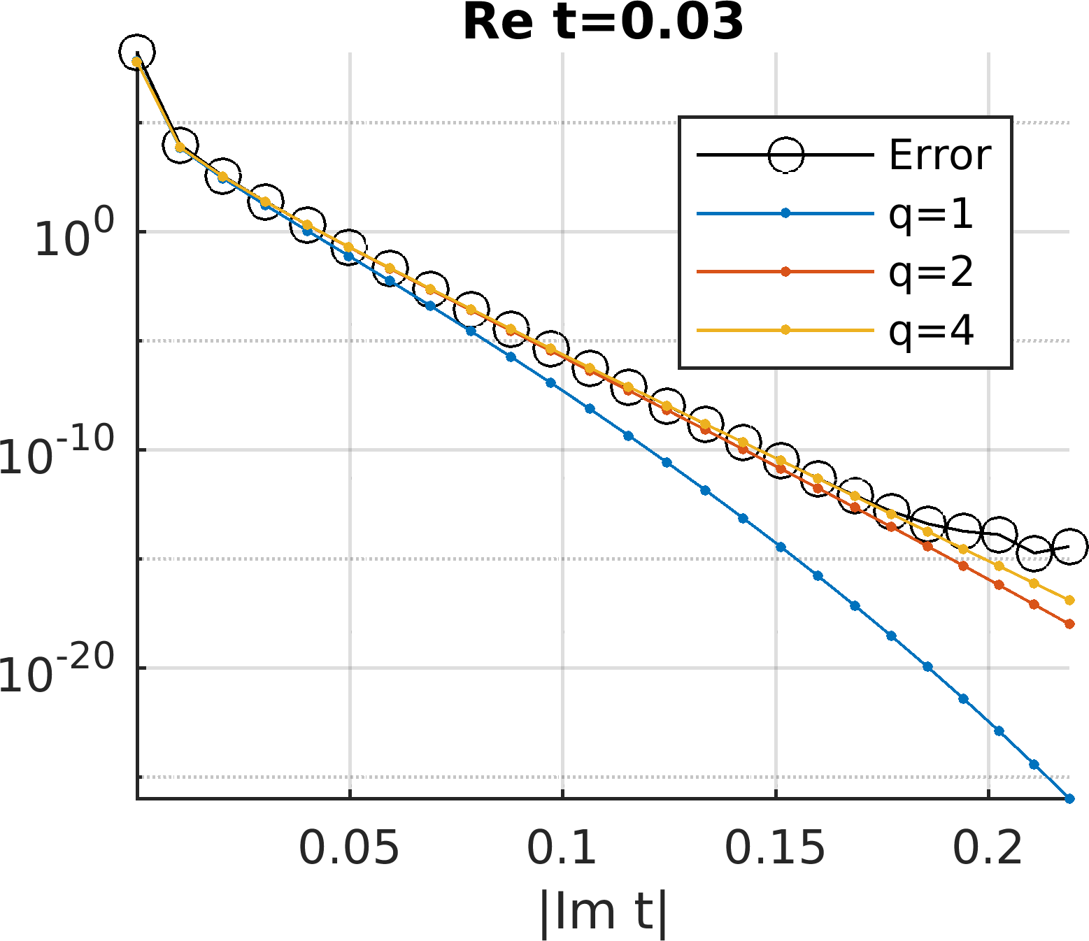
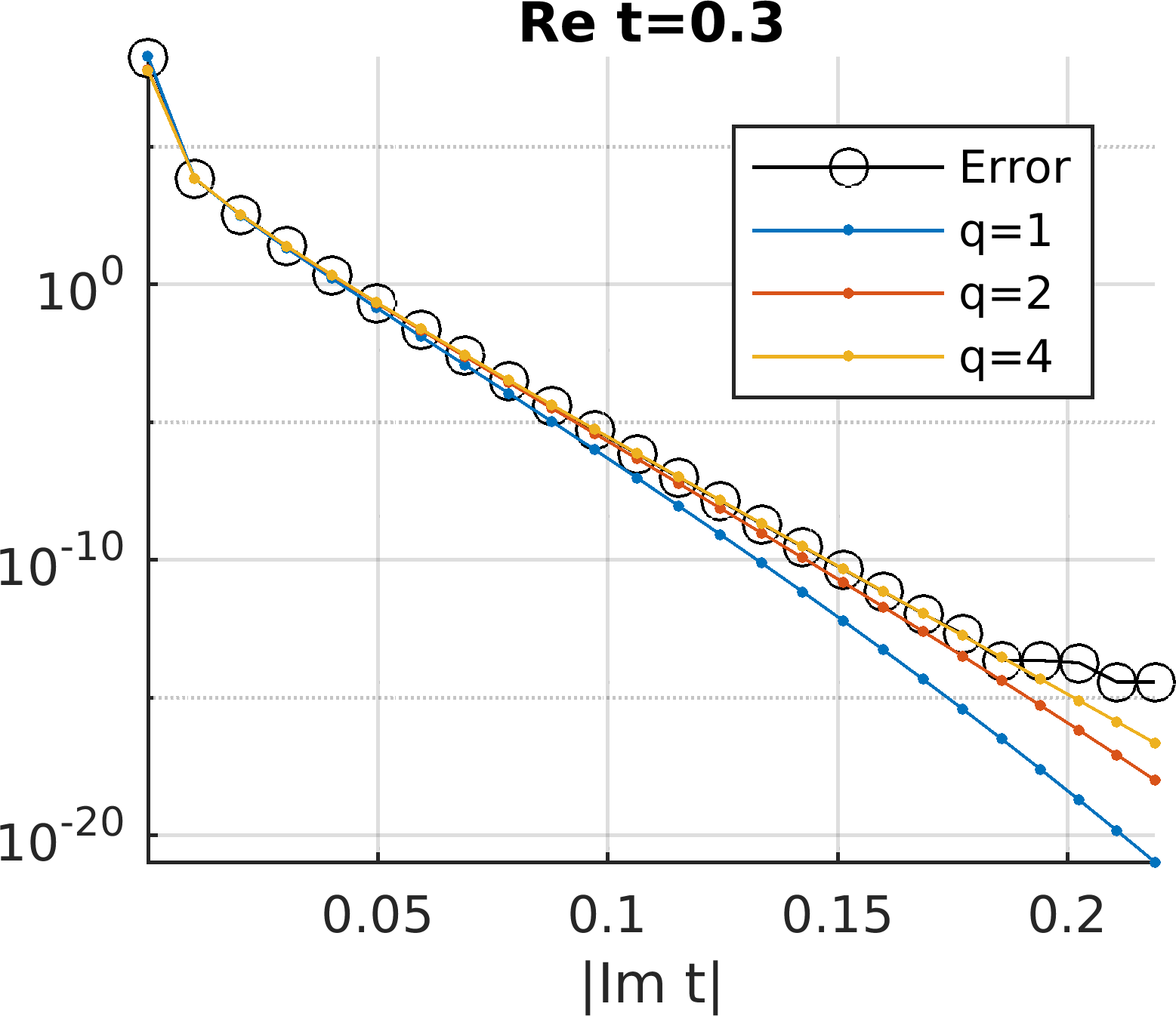
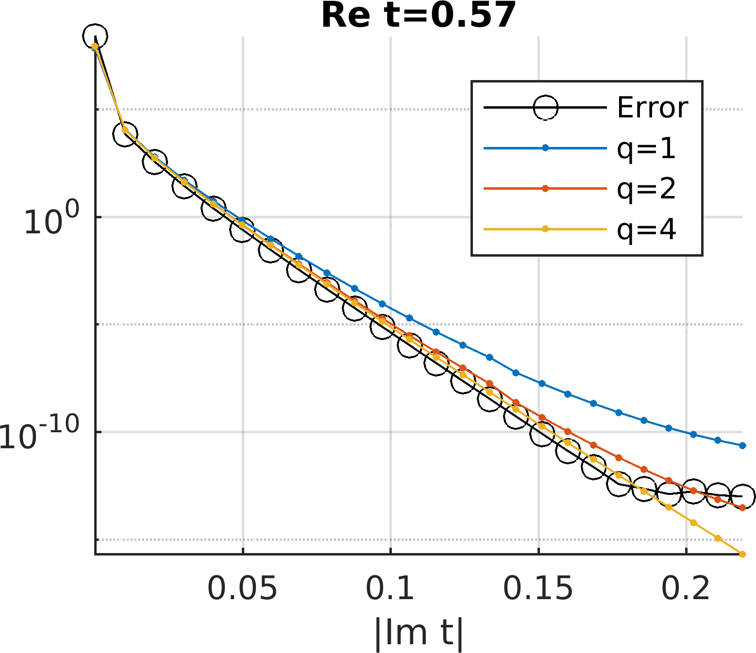
(d) Errors vs estimates, computed using $q=\{1,2,4\}$, on lines extending out from the curve. From left to right, the errors are computed on lines corresponding to $\operatorname{Re}t=\{0.03,0.3,0.57\}$.

Figure 8: Effects of using a local Taylor expansion of order $q$ for finding roots based on the trapezoidal rule discretization, on the problem shown in Figs. 4 and 5. Figures 8(a), 8(b) and 8(c) show the roots $t\in\mathbb{C}$ that are found when the method is applied to the points in the grid in Fig. 4(b) (the true roots are those shown in 4(a)). The “steps” occur where a different node on the curve is used as the expansion center. The plots in Fig. 8(d) focus on the thick black lines marked in the abovementioned plots, comparing the true error to the estimates computed using root finding of varying order. Clearly, $q\geq 2$ is sufficient for capturing the magnitude of the error, up to the point where roundoff starts to dominate.

5.5.1 Evaluating quantities at the root

So far we have derived the error estimates for one-dimensional curves, and discussed how to find the root $t_{0}$ that corresponds to $\bm{x}$. However, in order to evaluate the estimates, we also need the values $f(t_{0})$ and $G(t_{0})$. The geometry factor $G(t_{0})$, defined in (40), can easily be computed using the approximation $\tilde{\bm{\gamma}}$, which we have already constructed in order to find the root (it is in fact computed in the Newtons iterations).The value $f(t_{0})$ does not come “for free” in the same way, and the cheapest way to compute it is to simply bound it (approximately) using the maximum value on the curve, $f(t_{0})\lesssim\mathinner{\!\left\lVert f\right\rVert}_{\infty(\Gamma)}$, or on a section of the curve. Using the maximum value over the Gauss-Legendre panel generally works well, see comparison in [4, Fig. 4]. Slightly more accurate, and slightly more costly, is to construct an approximation $\tilde{f}$, in the same way that we constructed $\tilde{\bm{\gamma}}$, and then evaluate $\tilde{f}(t_{0})$. This is the method that we use in this paper.

5.6 Examples for one-dimensional curves in $\mathbb{R}^{3}$

The estimates that we have derived so far are for quadrature errors in layer potentials near one-dimensional curves. The most obvious use for these are in the context of boundary integral methods for planar geometries, but there is in fact nothing limiting them to 2D problems, as long as the source geometry is one-dimensional. In 3D, one-dimensional source geometries appear in slender-body approximations of fluid flow or electrical fields (see discussion in [2]). To demonstrate the application of our estimates on a curve in 3D, we consider a curve (shown in Fig. 9) defined on the surface known as the QAS3 stellarator [10]. This surface was used as an example for the integral equation solver developed in [13], and we will use it for our surface error estimates in Section 6.

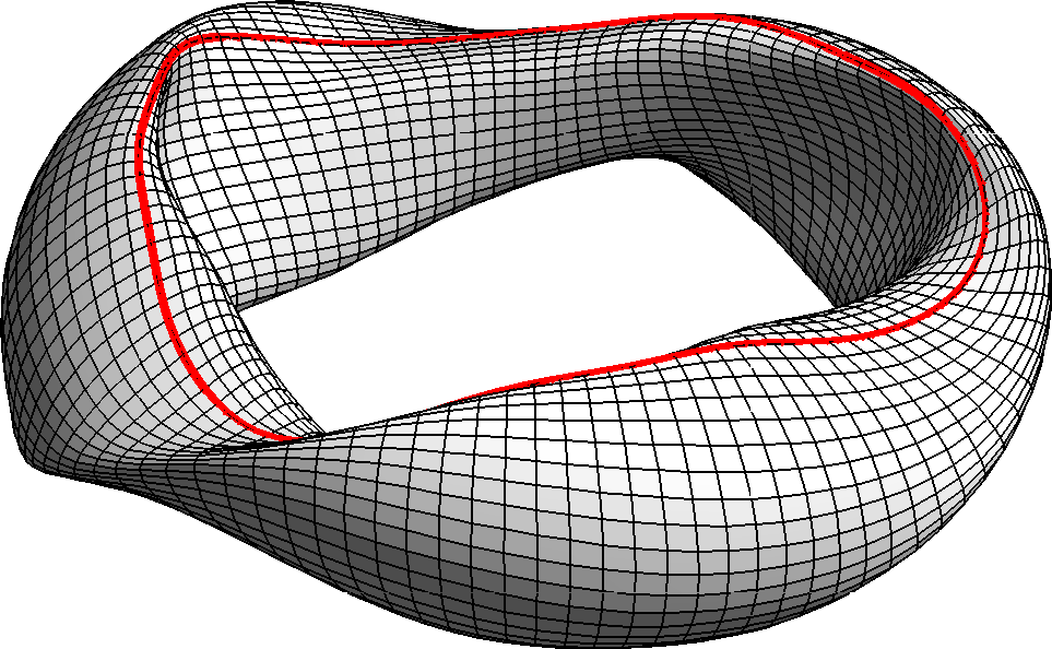
Figure 9: One-dimensional curve on the surface of the QAS3 stellarator.

On the QAS3 stellerator, we define a curve $\Gamma$ by fixing the poloidal angle at $\phi=\pi/2$. The curve is then parametrized in the toroidal angle $\theta\in[0,2\pi)$. We set our layer potential to be the 3D harmonic single layer potential $u(\bm{x})=S^{3D}_{H}[\sigma](\bm{x})$, given in (1), with the simple density $\sigma(\bm{y})=y_{1}y_{3}$. We discretize $\Gamma$ in two ways: using the trapezoidal rule with $n=120$, and using the composite Gauss-Legendre rule with 10 panels and $n=16$. Using these discretizations, we evaluate $u(\bm{x})$ on the plane $z=1.16$ (the mean $z$-coordinate of $\Gamma$). We compute the error using adaptive quadrature, and estimate the error using (61) and (80) with $p=1/2$. The root $t_{0}$ is for each target point found by approximating $\gamma$ using a 5th order Taylor expansion in the case of the trapezoidal rule, and a 16th order Legendre polynomial on each panel in the case of the Gauss-Legendre rule. The results, shown in Fig. 10, indicate that our estimates work well also for one-dimensional curves in 3D. The black spots in the blue area in Fig. 10(b) is due to the fact that the root finding process has not converged to the correct root for these evaluation points. This is not of practical concern, since these locations are far from the curve. See also the discussion in connection to Fig. 15(b).

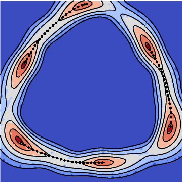
(a) Trapezoidal rule.

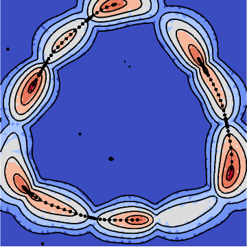
(b) Gauss-Legendre rule.

Figure 10: Quadrature errors (filled contours) vs error estimates (black contours) for the 3D harmonic single layer potential evaluated from the source line marked in Fig. 9. Errors are measured in the $xy$-plane for a fixed $z=1.16$.

6 Quadrature errors near two-dimensional surfaces in $\mathbb{R}^{3}$

Let us now consider the three-dimensional case, for which our prototype layer potential (7) takes the form (9). Here, $S\subset\mathbb{R}^{3}$ is a two-dimensional surface parametrized by $\bm{\gamma}\mathrel{\mathop{\ordinarycolon}}E\to\mathbb{R}^{3}$, $E=\{E_{1}\times E_{2}\}\subset\mathbb{R}^{2}$.

Our goal is now to find a way of estimating the error committed when (9) is evaluated using an $n_{s}\times n_{t}$ tensor product quadrature rule, based on the trapezoidal and/or Gauss Legendre quadrature rule. The base intervals $E_{1}$ and $E_{2}$ are set according to which rule is considered in the two directions. The use of the Gauss-Legendre rule means that we are considering one panel that only covers part of a full surface. To obtain the full error estimate, the error contribution from different panels must be added. Due to the localized nature of the errors, in practice, only the panels closest to the target point $\bm{x}$ need be considered.

6.1 Error estimates for surfaces

If we introduce the convenience notation $g_{p}=f/\mathinner{\!\left\lVert\bm{\gamma}-\bm{x}\right\rVert}^{2p}$, then we can write the tensor product quadrature as

$$\operatorname{Q}_{s,n_{s}}\operatorname{Q}_{t,n_{t}}g_{p} =\left(\operatorname{I}_{s}-\operatorname{E}_{s,n_{s}}\right)\left(\operatorname{I}_{t}-\operatorname{E}_{t,n_{t}}\right)g_{p}.$$ (89)

The operators $I[g]$, $Q_{n}[g]$ and $E_{n}[g]$ where introduced in the beginning of section 3. Here we use them with a subindex indicating if they are applied in the $s$ or the $t$ direction. For ease of notation, we have also skipped the brackets above, such that $I_{s}I_{t}g$ means an integration of $g$ first in the $t$ and then in the $s$ direction. The full expression of the term $\operatorname{I}_{s}\operatorname{E}_{t,n_{t}}g_{p}$ can be found in (91) below.

Neglecting the quadratic error term, and using that $\operatorname{E}_{s,n_{s}}\operatorname{I}_{t}=\operatorname{I}_{t}\operatorname{E}_{s,n_{s}}$, we can approximate the tensor product quadrature error as

$$\operatorname{E}^{2}_{n_{s},n_{t}}g_{p} \coloneqq\left(\operatorname{I}_{s}\operatorname{I}_{t}-\operatorname{Q}_{s,n_{s}}\operatorname{Q}_{t,n_{t}}\right)\,g_{p}\approx\left(\operatorname{I}_{s}\operatorname{E}_{t,n_{t}}+\operatorname{I}_{t}\operatorname{E}_{s,n_{s}}\right)\,g_{p}.$$ (90)

Elliott et al. [9] has shown for some basic integrals, that the remainder of the remainder term that we here neglect can have an important contribution. It is however a higher order contribution, and this is only true when the quadrature error is large, and we will proceed without it.

In essence, the formula above means that we can compute an approximation to the tensor product quadrature error by integrating the one-dimensional error estimates that we have already derived. To expand this statement, let us now focus on the first term of (90) (the second one is treated identically). We have that

$$\operatorname{I}_{s}\operatorname{E}_{t,n_{t}}g_{p}=\int_{E_{1}}\left[\int_{E_{2}}\frac{f(s,t)\operatorname{d\!}t}{\mathinner{\!\left\lVert\bm{\gamma}(s,t)-\bm{x}\right\rVert}^{2p}}-\sum_{l=1}^{n}\frac{f(s,t_{l})w_{l}}{\mathinner{\!\left\lVert\bm{\gamma}(s,t_{l})-\bm{x}\right\rVert}^{2p}}\right]\operatorname{d\!}s.$$ (91)

The term in the brackets (i.e. $\operatorname{E}_{t,n_{t}}$) represents the quadrature error on the line $L_{s}$ that for a given $s$ is defined as

$$L_{s}\coloneqq\left\{\bm{\gamma}(s,t)\mid t\in E_{2}\right\},\quad s\in E_{1}.$$ (92)

See illustration in Fig. 11. Estimating this error is precisely the problem that was treated in Section 5. As we have seen, the magnitude of the error depends on the closest root to the squared distance function, here defined as

$$R^{2}(s,t)\coloneqq\mathinner{\!\left\lVert\bm{\gamma}(s,t)-\bm{x}\right\rVert}^{2}.$$ (93)

For a given $s$, we denote by $t_{0}(s)$ the complex root such that

$$R^{2}\left(s,t_{0}(s)\right)=0.$$ (94)

In order to abbreviate our notation, let $\operatorname{est}(t_{0},n,p)$ denote the quadrature rule specific part of one of the estimates derived in Section 5, such that

$$|\operatorname{I}_{s}\operatorname{E}_{t,n_{t}}g_{p}|\leq\operatorname{I}_{s}|\operatorname{E}_{t,n_{t}}g_{p}|\approx\int_{E_{1}}\mathinner{\!\left\lvert f\left(s,t_{0}(s)\right)G\left(s,t_{0}(s)\right)^{p}\right\rvert}\operatorname{est}\left(t_{0}(s),n,p\right)\operatorname{d\!}s.$$ (95)

Since we are considering problems in three dimensions we assume that $p$ is a half-integer. Then we have from Error estimates 4 and 6 (Eqs. 61 and 80) that

$$\operatorname{est}(t_{0},n,p)=\frac{4\pi}{\Gamma(p)}\begin{cases}n^{p-1}e^{-n|\operatorname{Im}t_{0}|}&\quad\text{for trapezoidal,}\\ \mathinner{\!\left\lvert\frac{2n+1}{\sqrt{t_{0}^{2}-1}}\right\rvert}^{p-1}\rho(t_{0})^{-(2n+1)}&\quad\text{for Gauss-Legendre.}\end{cases}$$ (96)

Our task now is to evaluate the integral (95) (and the analogous integral to estimate $|\operatorname{I}_{t}\operatorname{E}_{s,n_{s}}g_{p}|$). The main difficulty in doing this is that even though we have a closed form expression for $\operatorname{est}(t_{0},n,p)$, we do not have one for $\operatorname{est}(t_{0}(s),n,p)$, since $t_{0}(s)$ is computed numerically using the technique outlined in 5.5. We could still evaluate (95) using quadrature, but that would require us to repeat the numerical root finding procedure multiple times for a single target point $\bm{x}$, something which we deem would be too costly for the purpose of error estimation. Instead, we use the following semi-analytical approach.

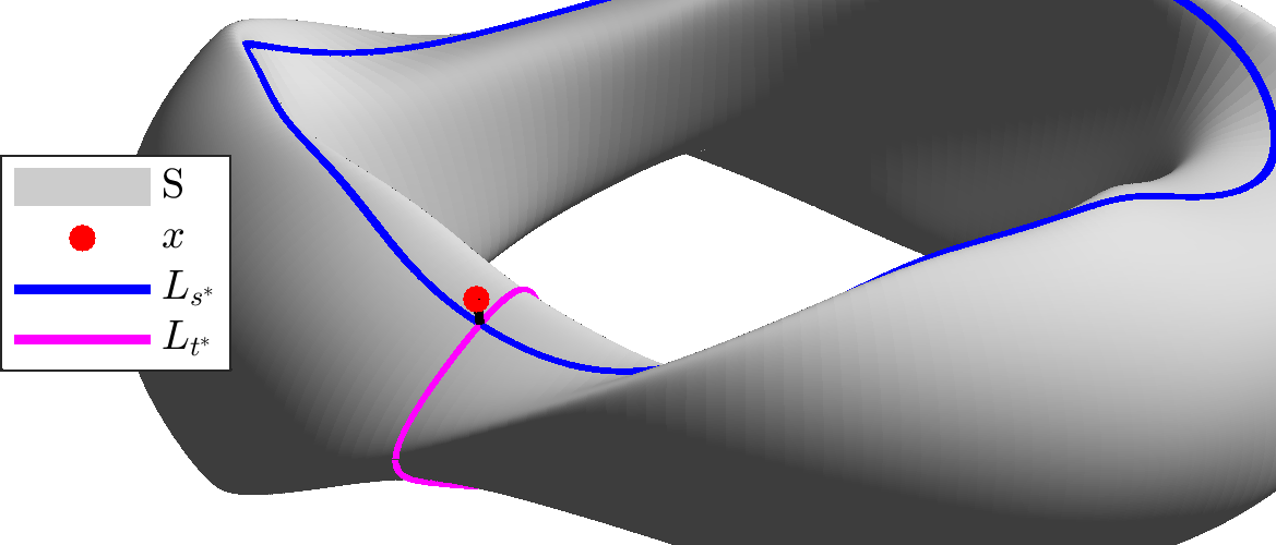
Figure 11: Lines $L_{s^{*}}$ and $L_{t^{*}}$ on the QAS3 stellarator, intersecting at the point $\bm{\gamma^{*}}=\bm{\gamma}(s^{*},t^{*})$. Here $s$ is the poloidal angle and $t$ is the toroidal angle.

6.1.1 Best approximation

In order to evaluate (95), our first step is to find the closest grid point on the surface, which we denote $\bm{\gamma^{*}}=\bm{\gamma}(s^{*},t^{*})$. At this location, we assume that we have access to the derivatives $\partial_{t}\bm{\gamma}$ through $\partial_{t}^{q}\bm{\gamma}$ (either analytically, or computed numerically at the time of discretization). Then we can form the univariate local approximation

$$\bm{\tilde{\gamma}}(s^{*},t)=\sum_{j=0}^{q}\frac{\left(t-t^{*}\right)^{j}}{j!}\mathinner{\dfrac{\partial{{}^{j}}\bm{\gamma}}{\partial{t^{j}}}}(s^{*},t^{*}).$$ (97)

Alternatively, we can form a global $n_{t}$th order polynomial approximation on the line $L_{s^{*}}$,

$$\bm{\tilde{\gamma}}(s^{*},t)=\operatorname{P}_{n}\left[\bm{\gamma}(s^{*},\cdot)\right](t).$$ (98)

Typically we use the latter approximation for Gauss-Legendre, since it is “global” only over a panel where $n$ is small, while we utilize the local approximation for the trapezoidal rule. We insert this (local or global) approximation into the squared distance function (93) and apply the techniques discussed in Section 5.5 to find the root

$$t_{0}^{*}\approx t_{0}(s^{*}).$$ (99)

This root represents our best approximation of $t_{0}(s^{*})$, where $s^{*}$ is the value of the parametrization in $s$ at the quadrature node that is closest to $\bf{x}$.

6.1.2 Linear approximation

We also form the bivariate linear approximation

$$\bm{{\tilde{\gamma}}}_{L}(s,t) =\bm{\gamma}^{*}+\partial_{s}\bm{\gamma}(s^{*},t^{*})\Delta s+\partial_{t}\bm{\gamma}(s^{*},t^{*})\Delta t,$$ (100)

where $\Delta t=t-t^{*}$ and $\Delta s=s-s^{*}$. For brevity we write $\bm{r}=\bm{\gamma}^{*}-\bm{x}$, $\bm{\gamma}^{*}_{s}=\partial_{s}\bm{\gamma}(s^{*},t^{*})$ and $\bm{\gamma}^{*}_{t}=\partial_{t}\bm{\gamma}(s^{*},t^{*})$. The squared distance function (93) then takes the form

$$R^{2}\approx\underbrace{\mathinner{\!\left\lVert\bm{r}\right\rVert}^{2}+2(\bm{r}\cdot\bm{\gamma}^{*}_{s})\Delta s+\mathinner{\!\left\lVert\bm{\gamma}^{*}_{s}\right\rVert}^{2}\Delta s^{2}}_{a(\Delta s)}+\underbrace{\left(2(\bm{r}\cdot\bm{\gamma}^{*}_{t})+2(\bm{\gamma}^{*}_{s}\cdot\bm{\gamma}^{*}_{t})\Delta s\right)}_{b(\Delta s)}\Delta t+\underbrace{\mathinner{\!\left\lVert\bm{\gamma}^{*}_{t}\right\rVert}^{2}}_{c(\Delta s)}\Delta t^{2}.$$ (101)

Finding the roots of this by solving for $\Delta t$, we get

$$t_{0}^{L}(\Delta s)=t^{*}-\frac{b}{2c}\pm i\frac{\sqrt{4ac-b^{2}}}{2c}.$$ (102)

This is our linear approximation to $t_{0}(s)$.

6.1.3 Combined approximation

Due to the exponential distance dependence of quadrature errors, we expect $\operatorname{est}(t_{0}(s),n,p)$ to have a peak close to $s^{*}$, and then decay exponentially with $|s-s^{*}|$. In order to capture the magnitude of that peak as well as possible, while having a simple explicit dependence on $s$, we define the following combined approximation:

$$\tilde{t}_{0}(s)=t_{0}^{*}-t_{0}^{L}(0)+t_{0}^{L}(s-s^{*}).$$ (103)

Inserting this into (95), and reasoning that $\operatorname{est}(t_{0}(s),n,p)$ is the most rapidly varying factor (with a peak near $s^{*}$),

$$\operatorname{I}_{s}|\operatorname{E}_{t,n_{t}}g_{p}|\approx\mathinner{\!\left\lvert f\left(s^{*},t_{0}^{*}\right)G\left(s^{*},t_{0}^{*}\right)^{p}\right\rvert}\int_{E_{1}}\operatorname{est}\left(t_{0}^{*}-t_{0}^{L}(0)+t_{0}^{L}(s-s^{*}),n,p\right)\operatorname{d\!}s.$$ (104)

We are now left with a definite integral of a closed-form function. Since we only need to compute it to 1–2 digits of accuracy, it can be rapidly evaluated using quadrature, the details of which depend on which estimate we are integrating, as outlined below. This completes our method for estimating quadrature errors in 3D. In 6.2 we summarize the required steps, and in 7 we demonstrate its performance.

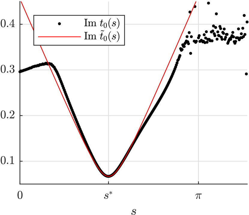
(a) The root $t_{0}(s)$ is computed numerically on the line $L_{s}$, while $\tilde{t}_{0}(s)$ is computed using the combined approximation (103).

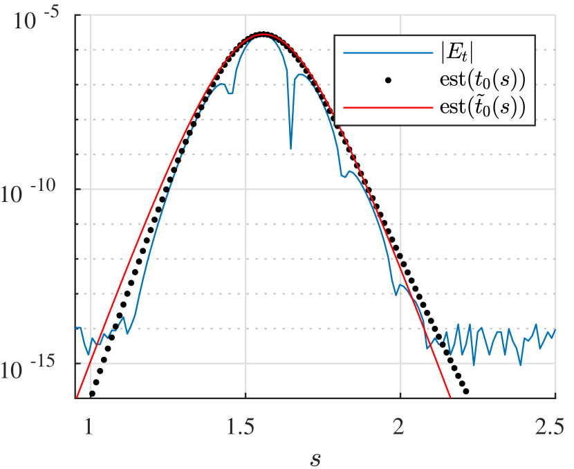
(b) Actual trapezoidal rule error $|\operatorname{E}_{t,n_{t}}|$ on the line $L_{s}$, compared to estimates computed using the roots in Fig. 12(a).

Figure 12: Quantities measured on the line marked $L_{t^{*}}$ in Fig. 11. Kernel is single layer.

Trapezoidal rule

In the case of the trapezoidal rule we are integrating the estimate (61) on the periodic interval $E_{1}=[0,2\pi)$. The linear approximation does not take the periodicity into account, so it is reasonable to use $\Delta s\in[-\pi,\pi]$ as the interval of integration. On this interval the estimate decays several orders of magnitude, since it loops around the entire geometry in physical space. Quantifying this decay, we have that (61) decays as $e^{-n~{}|\operatorname{Im}t_{0}|}$. For large $|s-s^{*}|$ the imaginary part of our linear approximation grows as

$$\mathinner{\!\left\lvert\operatorname{Im}t_{0}(s)\right\rvert}\sim k\mathinner{\!\left\lvert s-s^{*}\right\rvert},\quad k=\frac{\mathinner{\!\left\lVert\bm{\gamma}^{*}_{s}\right\rVert}}{\mathinner{\!\left\lVert\bm{\gamma}^{*}_{t}\right\rVert}},$$ (105)

so asymptotically the estimate decays as (temporarily omitting $n,p$ in the argument of $\operatorname{est}(.)$),

$$\operatorname{est}\left(t_{0}(s)\right)\sim e^{-nk~{}|s-s^{*}|}.$$ (106)

For our purposes (1–2 digits of accuracy) we can safely expand the interval of integration in (104) from $[-\pi,\pi]$ to $[-\infty,\infty]$, as the added tails are negligible,

$$\int_{E_{1}}\operatorname{est}\left(\tilde{t}_{0}(s)\right)\operatorname{d\!}s\approx\int_{0}^{\infty}\operatorname{est}\left(\tilde{t}_{0}(s^{*}+\Delta s)\right)\operatorname{d\!}\,(\Delta s)+\int_{0}^{\infty}\operatorname{est}\left(\tilde{t}_{0}(s^{*}-\Delta s)\right)\operatorname{d\!}\,(\Delta s).$$ (107)

Then, Gauss-Laguerre quadrature is suitable, as it is a Gaussian quadrature rule for integrals of the type $\int_{0}^{\infty}g(x)e^{-x}\operatorname{d\!}x$ [15, §3.5(v)]. Substituting $x=nk\Delta s$,

$$\int_{0}^{\infty}\operatorname{est}\left(\tilde{t}_{0}(s^{*}\pm\Delta s)\right)\operatorname{d\!}\,(\Delta s) =\frac{1}{nk}\int_{0}^{\infty}\ \underbrace{\left[\operatorname{est}\left(\tilde{t}_{0}(s^{*}\pm x/nk)\right)e^{x}\right]}_{h^{\pm}(x)}e^{-x}\operatorname{d\!}x.$$ (108)

We find that it is sufficient to apply 8-point Gauss-Laguerre quadrature to $h^{\pm}(x)$.

Gauss-Legendre rule

The integration of in (104) is more straightforward in the case of the Gauss-Legendre estimate (80), where the interval $E_{1}=[-1,1]$ runs between the edges of a panel in the neighborhood of the target point $\bm{x}$. Here we have found that it is sufficient to use Gauss-Legendre quadrature with 8 points to evaluate (104). Depending on the location of $s^{*}$, this is done using either two 4-point rules or one 8-point rule,

$$\int_{-1}^{1}=\begin{cases}\int_{-1}^{s^{*}}+\int_{s^{*}}^{1}&\text{ if }|s^{*}|<0.9,\\ \int_{-1}^{1}&\text{ otherwise }.\end{cases}$$ (109)

We remark that the second case above is applicable to the case also where $s^{*}<-1$ and $>1$, which would typically occur when the target point $\bm{x}$ is closest to a neighboring panel.

6.2 Summary of algorithm for error estimation near surfaces

We now summarize our algorithm for quadrature error estimation near surfaces: Given a layer potential of the form (9) with a half-integer $p$, evaluated at a target point $\bm{x}$, the quadrature error due to a near singularity in the integrand can be accurately estimated through the following steps:

1. Identify the grid point $\bm{\gamma}^{*}=\bm{\gamma}(s^{*},t^{*})$ on $S$ that is closest to $\bm{x}$, see eq. (88).

2. Form $\bm{\tilde{\gamma}}(s^{*},t)$ using either a local (97) or a global (98) approximation.

3. Use Newton’s method to find $t_{0}^{*}$ such that $\mathinner{\!\left\lVert\bm{\tilde{\gamma}}(s^{*},t_{0}^{*})-\bm{x}\right\rVert}^{2}=0$, as outlined in Section 5.5. Evaluate $G(s^{*},t_{0}^{*})$ (already computed in the Newton iterations), as this quantity is used in the evaluation of the error estimate.

4. Compute an approximation to $f(s^{*},t_{0}^{*})$, either as $\mathinner{\!\left\lVert f\right\rVert}_{\infty(S)}$, or through $\tilde{f}(s^{*},t)$ formed using the same kind of approximation used for $\bm{\tilde{\gamma}}$ in step 2.

5. Form the combined root approximation $\tilde{t}_{0}(s)$ defined in (103), using (101) and (102) together with $t_{0}^{*}$ and $\bm{\gamma}^{*}_{s},\bm{\gamma}^{*}_{t}$.

6. Compute $\operatorname{I}_{s}|\operatorname{E}_{t,n_{t}}g_{p}|$ through numerical integration of (104) as outlined in Section 6.1.3, with $\operatorname{est}(t_{0})$ given by (96), and using the quantities $G(s^{*},t_{0}^{*})$, $f(s^{*},t_{0}^{*})$, and $\tilde{t}_{0}(s)$ from previous steps.

7. Compute $\operatorname{I}_{t}|\operatorname{E}_{s,n_{s}}g_{p}|$ by repeating steps 2–6 with the roles of $s$ and $t$ interchanged.

8. Estimate the quadrature error at $\bm{x}$ as

   $$|\operatorname{E}^{2}_{n_{s},n_{t}}g_{p}|\approx\operatorname{I}_{s}|\operatorname{E}_{t,n_{t}}g_{p}|+\operatorname{I}_{t}|\operatorname{E}_{s,n_{s}}g_{p}|.$$ (110)

9. (In the case of panel-based Gauss-Legendre quadrature, repeat the above steps for all panels $S$ close to $\bm{x}$ and sum the contributions.)

7 Numerical experiments for a surface in $\mathbb{R}^{3}$

We will now show that the method of Section 6 can be used for accurately estimating the nearly singular quadrature error when evaluating a layer potential from a surface in three dimensions.

In Table 1 we identify the corresponding kernels and $p$ in the integral (7) for different PDEs. Here we consider only scalar kernels, but the method can be directly applied also to tensorial kernels, where the estimates are applied component by component to the vectorial output. From this, the function $f(s,t)$ introduced in (9) and used in the error estimates can easily be identified.

$u(\bm{x})=\int_{S}\frac{k\left(\bm{x},\bm{y}\right)\sigma(\bm{y})}{\mathinner{\!\left\lVert\bm{y}-\bm{x}\right\rVert}^{2p}}\operatorname{d\!}S(\bm{y})$
PDE	Single layer, $p=1/2$	Double layer, $p=3/2$
		$k\left(\bm{x},\bm{y}\right)=\tilde{k}\left(\bm{x},\bm{y}\right){\bm{n}_{y}}\cdot(\bm{y}-\bm{x})$
Harmonic
$\Delta u=0$	$k\left(\bm{x},\bm{y}\right)=1$	$\tilde{k}\left(\bm{x},\bm{y}\right)=1$
Helmholtz
$(\Delta+\omega^{2})u=0$	$k\left(\bm{x},\bm{y}\right)=e^{i\omega\mathinner{\!\left\lVert\bm{y}-\bm{x}\right\rVert}}$	$\tilde{k}\left(\bm{x},\bm{y}\right)=(i\omega\mathinner{\!\left\lVert\bm{y}-\bm{x}\right\rVert}-1)e^{i\omega\mathinner{\!\left\lVert\bm{y}-\bm{x}\right\rVert}}$
Mod. Helmholtz
$(\Delta-\omega^{2})u=0$	$k\left(\bm{x},\bm{y}\right)=e^{-\omega\mathinner{\!\left\lVert\bm{y}-\bm{x}\right\rVert}}$	$\tilde{k}\left(\bm{x},\bm{y}\right)=(-\omega\mathinner{\!\left\lVert\bm{y}-\bm{x}\right\rVert}+1)e^{-\omega\mathinner{\!\left\lVert\bm{y}-\bm{x}\right\rVert}}$

Table 1: PDEs with corresponding single and double layer kernels, identifying the functions $k$ and the values of $p$ for integrals written in the form (7).

As our source geometry we will use the QAS 3 stellarator [10] that was used in Section 5.6. We discretize the surface in two ways: using the tensor product trapezoidal rule with $50\times 150$ points, and using a $12\times 36$ grid of quadrilateral panels, each discretized with an $8\times 8$ tensor product Gauss-Legendre rule. These two discretizations are shown in Fig. 13. We choose to start to evaluate the 3D harmonic double layer potential (in the form of (9), with $p=3/2$)

$$D^{3D}_{H}[\sigma](\bm{x})=\int_{S}\sigma(\bm{y})\frac{{\bm{n}_{y}}\cdot(\bm{y}-\bm{x})}{\mathinner{\!\left\lVert\bm{y}-\bm{x}\right\rVert}^{3}}\,\,\operatorname{d\!}S(\bm{y}),$$ (111)

with the (arbitrarily chosen) density

$$\sigma(\bm{y})=\sigma(\bm{\gamma}(s,t))=1+\cos(s)\sin(t).$$ (112)

This density is illustrated in Fig. 16. We could instead have used a layer density that is the actual solution to a corresponding integral equation, such that the layer potential (111) would produce the solution to a specific Laplace boundary value problem. This is what was done in section 4.1, for 2D results. Our experience is however that the density does not influence the nearly singular quadrature error much, as long as it is well resolved by the discretization. In 2D, the integral equation for the layer density $\sigma$ can be discretized by the regular Gauss-Legendre or trapezoidal rule. In 3D however, the integrand has a singularity, and a special quadrature method is needed to obtain accurate results. By specifying the density, we avoid any pollution from errors in the density as well as building the infrastructure for the accurate solution of the integral equation.

In all our tests, we compute the layer potential error by comparing with a potential computed using a grid with twice as many points in each direction. This choice of reference is cost effective in 3D, and sufficient for our purposes since we only need to know the error to within 1–2 digits of accuracy. The error is then compared to the estimate computed using the algorithm outlined in Section 6.2, with $p=3/2$. Just as in Section 5.6, $\bm{\tilde{\gamma}}$ is constructed using a 5th order Taylor expansion in the case of the trapezoidal rule.

In order to illustrate how our estimates perform, we will below report the results on several different sets of measurement points.

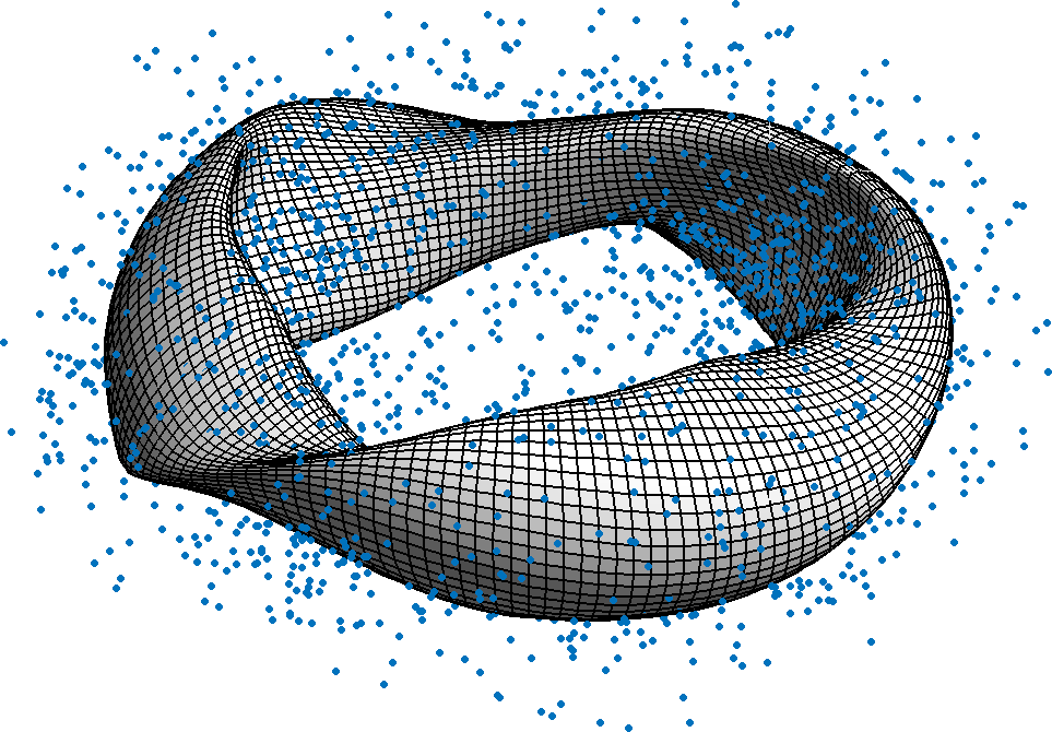
(a) Trapezoidal rule discretization with 3000 random test points.

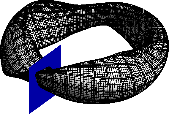
(b) Gauss-Legendre discretization with test points on a plane cutting the surface.

Figure 13: The QAS3 stellarator geometry used in our tests, showing two of the discretizations and test point distributions.

7.1 Random test points

As our first test, we compute the layer potential error at 3000 random points located in both the interior and exterior of the stellarator surface. The random points are generated by going a random distance in the normal direction from a random point on the surface,

$$\bm{x}=\gamma(s,t)+d\bm{n}(s,t),$$ (113)

with $(s,t,d)$ uniformly distributed random variables,

$$(s,t,d)\sim~{}\mathcal{U}(0,2\pi)\times\mathcal{U}(0,2\pi)\times\mathcal{U}(-h,h)\quad\mbox{ with }h=1.5~{}.$$ (114)

This results in the cloud of test points shown in Fig. 13(a), although it must be noted that only the exterior points are visible in the figure.

At each of the 3000 test points and for each of the two discretizations, we compute the error in the layer potential and compare it to our error estimate. This data is then used to generate the scatter plots shown in Fig. 14. These plots indicate that our estimates have the following important features:

• They are conservative most of the time (i.e. they overestimate the error). Only at a few points close to the surface where the errors are large do they slightly underestimate the error.

• They are within a factor 10 of the actual error most of the time.

• Starting at errors as small as around $10^{-15}$ for trapezoidal and $10^{-10}$ for Gauss-Legendre, the estimates never underestimate the error by more than a factor 10.

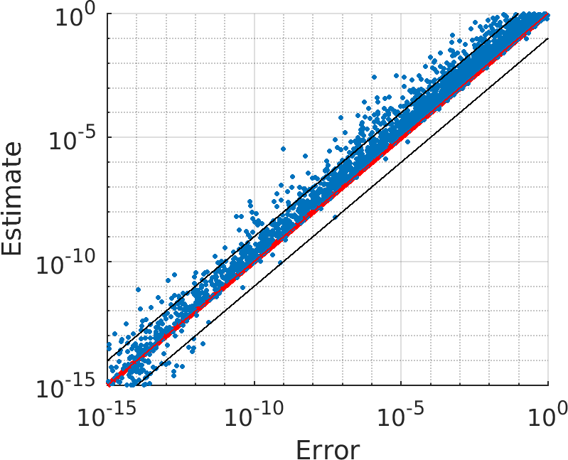
(a) Trapezoidal

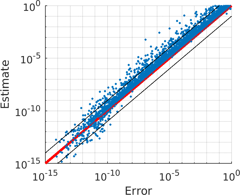
(b) Gauss-Legendre

Figure 14: Scatter plot of error vs estimate on the random points shown in Fig. 13(a). The red line indicates where error and estimate are equal, while the black lines indicate where they differ by factors $10$ and $1/10$, respectively.

7.2 Flat plane cutting the surface

As our second test, we compare errors and estimate on a set of $100\times 100$ points covering the square plane shown in Fig. 13(b). The results, displayed in Fig. 15, show that our estimates predict the error levels very well close to the surface, which is where one would normally want to use error estimates. However, the accuracy of the Gauss-Legendre estimate (Fig. 15(b)) deteriorates far away from the surface, meaning that the root finding process has not converged to the correct root. This is likely because the 8th order local polynomials used in the root finding get inaccurate that far away (using higher order panels would most likely yield better results). This is however far enough away from the surface that error estimates would typically not be applied, it is close to the surface that the error estimates are critical. Note that there are also a few isolated points in Fig. 15(a), where the error is overestimated. We can not explain why the root finding has failed in these locations. The results found here do support the conclusions made in the previous subsection, when discussing the results in figure 14.

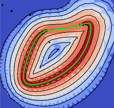
(a) Trapezoidal

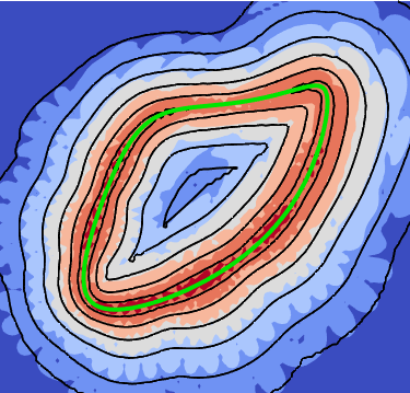
(b) Gauss-Legendre

Figure 15: Results on the plane shown in Fig. 13(b) for the two discretization, with the surface cross section marked green. The errors are shown as colored fields, with the contours of the estimates drawn in black for the levels $10^{\{-12,-10,-8,-6,-4,-2,0\}}$.

7.3 Toroidal shell

As our final test, we let our tests points be a grid of $200\times 76$ points on the surface of a torus with major radius $R=4.5$ and minor radius $r=1.7$, shown in Fig. 16. This surface, which we denote the toroidal shell, encloses the stellarator from which the layer potential is evaluated.

We tested the performance of the estimates on different kernels (see Table 1): the behaviour of the error and of the corresponding estimates depends on the decay of the singularity, so the plots will look very similar for kernels with the same decay. In addition to the results for the harmonic double layer potential (Fig. 17), in Fig. 18 we show also the erros and error estimates for the modified Helmholtz single layer potential with $\omega=5$ and the same discretization and density as shown in Fig. 16.

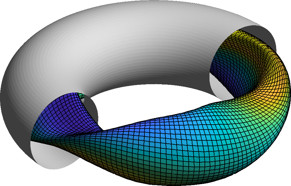
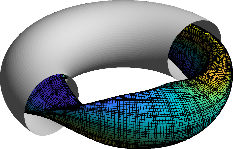
Figure 16: Toroidal shell on which we compute quadrature errors and estimates (note that only half the shell is shown here). The coloring of the stellarator surface corresponds to the density $\sigma$ given by (112).

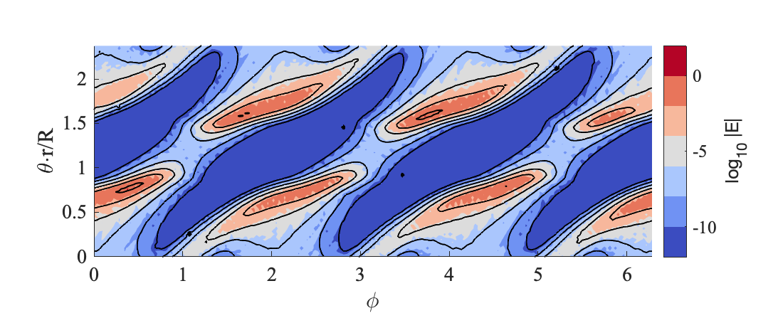
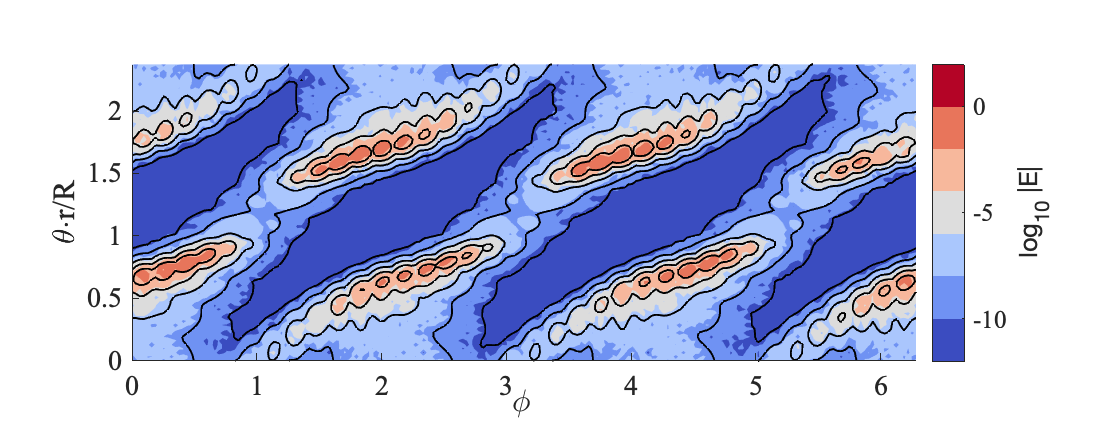
Figure 17: Errors for the harmonic double layer potential as colored fields and estimates as black contours on the toroidal shell, for the trapezoidal rule (above) and the Gauss-Legendre rule (below). The contours are drawn for the error levels $10^{\{-10,-8,-6,-4,-2,0\}}$. Note that the poloidal angle (vertical axis) is scaled by the aspect ratio of the torus.

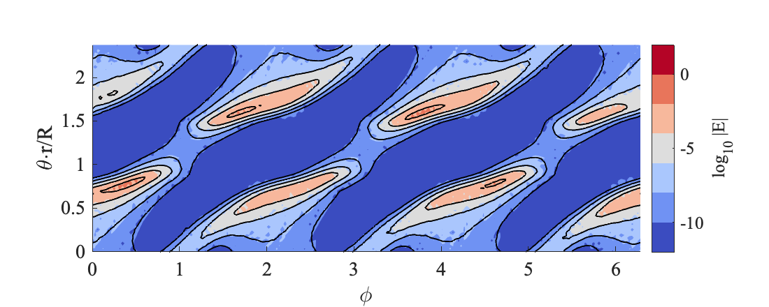
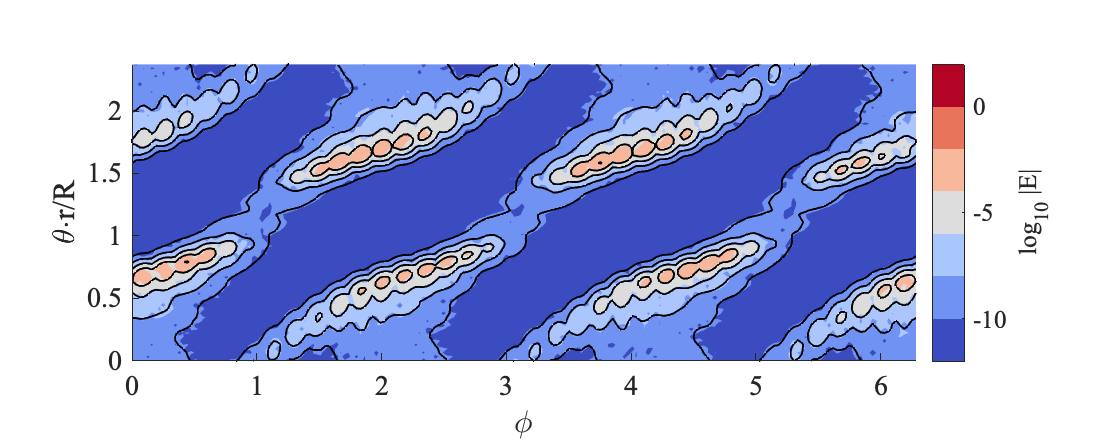
Figure 18: Errors for the single layer potential of the modified Helmholtz equation with $\omega=5$ as colored fields and estimates as black contours on the toroidal shell, for the trapezoidal rule (above) and the Gauss-Legendre rule (below). The contours are drawn for the error levels as in Figure 17.

8 Conclusions

In this paper we have introduced a theoretical and computational framework for estimating nearly singular quadrature errors in the evaluation of layer potentials of the form (7), for smooth source geometries that are either one-dimensional curves in $\mathbb{R}^{2}$ or $\mathbb{R}^{3}$, or two-dimensional surfaces in $\mathbb{R}^{3}$. This framework is defined for the trapezoidal and composite Gauss-Legendre quadrature rules, which are two of the most common choices in the integral equation field. However, generalization to other quadrature rules is possible with the knowledge of the remainder function $k_{n}$ (Elliott et al. derive an expression for Clenshaw-Curtis quadrature in [7]).

Our work on quadrature error estimates started in [3]. It was extended and improved upon for one-dimensional curves discretized using composite Gauss-Legendre quadrature in [4], e.g. introducing the root-finding procedure needed for accurate estimation for curved panels. In [2], a so-called singularity swap quadrature method was introduced for curves in both $\mathbb{R}^{2}$ and $\mathbb{R}^{3}$ again based on composite Gauss-Legendre quadrature, introducing some key ideas for curves in $\mathbb{R}^{3}$ that we have explored in this work.

There are three major contributions of the current work: (1) Showing how error estimation and root finding on one-dimensional curves can be derived for and applied to the trapezoidal rule, (2) extending the analysis for complex kernels on curves in $\mathbb{C}^{2}$ to real valued kernels on curves in both $\mathbb{R}^{2}$ and $\mathbb{R}^{3}$, (3) deriving the desired quadrature error estimates for two-dimensional surfaces in $\mathbb{R}^{3}$ building on the results on one-dimensional curves in $\mathbb{R}^{3}$.

As we have shown, our quadrature error estimates perform very well in actual computations, consistently estimating the error to within one order of magnitude of the actual value for layer potentials evaluated over curved surfaces in $\mathbb{R}^{3}$. For curves, the estimates are remarkably precise already for moderate values of discretization points $n$, even though they are asymptotic estimates. The focus of this work has not been to derive upper bounds of the error, even if such bounds would be desirable. Error estimates without unknown coefficients are more useful in actual simulations. Evaluation of our estimates have a low per-point computational cost, since they only require information from nearby surface grid points (if local approximations are used). They can therefore be used on the fly in 2D and 3D simulations to determine e.g. when the regular quadrature ceases to be sufficiently accurate or what upsamplig rate should be used. The error estimates can also be used to create adaptive quadrature algorithms, such as was done in 2D [4], especially needed in 3D applications with multiple particles interacting (e.g. drops [18, 19], vesicles [17], etc.) to provide efficient quadrature methods with error control.

Appendix A Two lemmas

In the derivation for half-integers in Section 5.1.2, we use a result that we prove in Lemma 2. We start by providing an intermediate result.

Lemma 1.

Let $\bar{p}\geq 1$ be an integer. Then the following holds,

$$\Gamma(1/2)\prod_{q=1}^{\bar{p}}\left(\bar{p}+1/2-q\right)=\Gamma(\bar{p}+1/2),$$ (115)

where $\Gamma(z)$ is the gamma function.

Proof: First make the simple substitution $r=\bar{p}-q$ to obtain

$$\Gamma(1/2)\prod_{q=1}^{\bar{p}}\left(\bar{p}+1/2-q\right)=\Gamma(1/2)\prod_{r=0}^{\bar{p}-1}\left(r+1/2\right).$$ (116)

We then make use of the relation $z\Gamma(z)=\Gamma(z+1)$, that holds for all $z\in\mathbb{C}$ (see e.g. Eqn 1.2.1 in [12]). Particularly, this yields

$$\frac{2\bar{p}+1}{2}\Gamma\left(\frac{2\bar{p}+1}{2}\right)=\Gamma\left(\frac{2\bar{p}+3}{2}\right),$$ (117)

and so $\frac{1}{2}\,\Gamma(1/2)=\Gamma(3/2)$, $\frac{3}{2}\,\Gamma(3/2)=\Gamma(5/2)$ etc. Starting from (116), we use this formula repeatedly,

$$\Gamma(1/2)\prod_{r=0}^{\bar{p}-1}\left(r+1/2\right) =\Gamma(1/2)\cdot(1/2)\prod_{r=1}^{\bar{p}-1}\left(r+1/2\right)=\Gamma(3/2)\prod_{r=1}^{\bar{p}-1}\left(r+1/2\right)=\cdots=$$

$$=\Gamma(\bar{p}-1+1/2)\cdot(\bar{p}-1+1/2)=\Gamma(\bar{p}+1/2),$$

which yields the desired result.

Lemma 2.

Let $\bar{p}\geq 1$ be an integer. Then the following holds,

$$\frac{1}{\prod_{q=1}^{\bar{p}}\left(-\bar{p}-1/2+q\right)}=\frac{1}{\sqrt{\pi}}\Gamma(1-(\bar{p}+1/2)),$$ (118)

where $\Gamma(z)$ is the gamma function.

Proof: We can factor out a negative sign, and use Lemma 1 together with the fact that $\Gamma(1/2)=\sqrt{\pi}$, to get

$$\frac{1}{\prod_{q=1}^{\bar{p}}\left(-\bar{p}-1/2+q\right)}=\frac{(-1)^{\bar{p}}}{\prod_{q=1}^{\bar{p}}\left(\bar{p}+1/2-q\right)}=\frac{(-1)^{\bar{p}}\sqrt{\pi}}{\Gamma(\bar{p}+1/2)}.$$ (119)

The so called Euler reflection formula (see e.g. Eqn 1.2.2 in [12]) holds for all $z\in\mathbb{C}$,

$$\Gamma(z)\Gamma(1-z)=\frac{\pi}{\sin(\pi z)}.$$ (120)

Specifically, this means that we have

$$\frac{1}{\Gamma(\bar{p}+1/2)}=\frac{(-1)^{\bar{p}}}{\pi}\Gamma(1-(\bar{p}+1/2)).$$ (121)

Combining this with (119), we obtain the desired result (118).

Appendix B Error estimates for cartesian and complex formulation of the harmonic double layer potential

The harmonic double layer potential in two dimensions is given by

$$u(\bm{x})=\int_{\Gamma}\frac{\bm{\hat{}}{\bm{n}}_{y}\cdot(\bm{x}-\bm{y})}{\mathinner{\!\left\lVert\bm{y}-\bm{x}\right\rVert}^{2}}\sigma(\bm{y})\operatorname{d\!}S(\bm{y}),$$ (122)

where $\hat{\bm{n}}_{y}$ is the outward pointing normal at $\bm{y}\in\Gamma$. With the curve parameterized by $\bm{\gamma}(t)\mathrel{\mathop{\ordinarycolon}}\mathbb{R}\rightarrow\mathbb{R}^{2}$, we have $\operatorname{d\!}S(\bm{y})=\mathinner{\!\left\lVert\bm{\gamma}^{\prime}(t)\right\rVert}\operatorname{d\!}t$.

Identify the vectors $\bm{x}$, $\bm{y}$ and $\hat{\bm{n}}_{y}$ in $\mathbb{R}^{2}$ by $z$, $\tau$ and $n_{\tau}$ in $\mathbb{C}$. We can then write

$$\frac{\bm{\hat{}}{\bm{n}}_{y}\cdot(\bm{x}-\bm{y})}{\mathinner{\!\left\lVert\bm{y}-\bm{x}\right\rVert}^{2}}\rightarrow\frac{\operatorname{Re}\left\{n_{\tau}\overline{(z-\tau)}\right\}}{(z-\tau)\overline{(z-\tau)}}=\operatorname{Re}\left\{\frac{n_{\tau}\overline{(z-\tau)}}{(z-\tau)\overline{(z-\tau)}}\right\}=\operatorname{Re}\left\{\frac{n_{\tau}}{z-\tau}\right\}.$$ (123)

Now let $\tau(t)\mathrel{\mathop{\ordinarycolon}}\mathbb{R}\rightarrow\mathbb{C}$ be a complex parameterization of $\Gamma$, a positively oriented curve. The outward pointing normal vector is then given by $n_{\tau}=-i\tau^{\prime}(t)/|\tau^{\prime}(t)|$. Furthermore, the integration element $\operatorname{d\!}S(\bm{y})=\mathinner{\!\left\lVert\bm{\gamma}^{\prime}(t)\right\rVert}\operatorname{d\!}t$ becomes $|\tau^{\prime}(t)|\operatorname{d\!}t=|\operatorname{d\!}\tau|$. This means that we can replace $\operatorname{d\!}S(\bm{y})$ by $\frac{-i}{n_{\tau}}\operatorname{d\!}\tau=\operatorname{Re}\left\{\frac{-i}{n_{\tau}}\operatorname{d\!}\tau\right\}$. Using also that $\sigma(\tau)$ is a real quantity, we get

$$u(z)=\operatorname{Re}\left\{\int\frac{n_{\tau}}{z-\tau}\sigma(\tau)\frac{-i}{n_{\tau}}\operatorname{d\!}\tau\right\}=\operatorname{Re}\left\{-i\int\frac{\sigma(\tau)}{z-\tau}\operatorname{d\!}\tau\right\}.$$ (124)

Hence, we can also write

$$u(z)=\operatorname{Im}\left\{\int\frac{\sigma(\tau)}{z-\tau}\operatorname{d\!}\tau\right\}=\int\sigma(\tau)\operatorname{Im}\left\{\frac{\operatorname{d\!}\tau}{z-\tau}\right\}$$ (125)

Now, we want to consider the error estimates that have been derived for the two different forms. For the complex form in (125) we can identify $g(t)$ in (26) with $g(t)=\sigma(t)$, if we ignore taking the imaginary part. For $p=1$, the error estimate (27) for approximating (125) then simply reads

$$|E_{n}^{Complex}|\approx\mathinner{\!\left\lvert\sigma(t_{0})k_{n}(t_{0})\right\rvert}.$$ (126)

Here, $k_{n}(.)$ is specific for the quadrature rule used and can be found in (20) and (18) for the trapezoidal rule and Gauss-Legendre quadrature, respectively.

The cartesian form of the double layer potential in (122) can be written in the form of (8) with $p=1$ and

$$f(t)=\bm{\hat{}}{\bm{n}}_{t}\cdot(\bm{x}-\bm{\gamma}(t))\,\sigma(t)\mathinner{\!\left\lVert\bm{\gamma}^{\prime}(t)\right\rVert}.$$ (127)

The error estimate (43) reads

$$\mathinner{\!\left\lvert E_{n}^{Cartesian}\right\rvert} \approx 2\mathinner{\!\left\lvert f(t_{0})G(t_{0})k_{n}(t_{0})\right\rvert}.$$ (128)

Using that

$$\hat{\bm{n}}_{t}=\frac{(-\gamma^{\prime}_{2}(t),\gamma^{\prime}_{1}(t))}{\mathinner{\!\left\lVert\bm{\gamma}^{\prime}(t)\right\rVert}},$$ (129)

we can write the product

$$\begin{split}f(t)G(t)&=\frac{-(-\gamma^{\prime}_{2}(t),\gamma^{\prime}_{1}(t))\cdot(\bm{x}-\bm{\gamma}(t))}{2\bm{\gamma}^{\prime}(t)\cdot\left(\bm{x}-\bm{\gamma}(t)\right)}\,\sigma(t)\\ &=\frac{1}{2}\frac{\gamma^{\prime}_{2}(t)(x_{1}-\gamma_{1}(t))-\gamma^{\prime}_{1}(t)(x_{2}-\gamma_{2}(t))}{\gamma^{\prime}_{1}(t)(x_{1}-\gamma_{1}(t))+\gamma^{\prime}_{2}(t)(x_{2}-\gamma_{2}(t))}\sigma(t)\end{split}$$ (130)

We have $R^{2}(t_{0},\bm{x})=(\gamma_{1}(t_{0})-x_{1})^{2}+(\gamma_{2}(t_{0})-x_{2})^{2}=0$. From this, we find

$$(\gamma_{1}(t_{0})-x_{1})=\pm i(\gamma_{2}(t_{0})-x_{2}),$$ (131)

and at $t=t_{0}$ the expression above simplifies to

$$f(t_{0})G(t_{0})=\pm\frac{i}{2}\sigma(t_{0}).$$ (132)

Hence, the error estimate (128) simplifies to

$$\mathinner{\!\left\lvert E_{n}^{Cartesian}\right\rvert} \approx\mathinner{\!\left\lvert\sigma(t_{0})k_{n}(t_{0})\right\rvert},$$ (133)

which is identical to the error estimate for the complex kernel in (126).

In writing the estimate for the complex integral, we did not take into account that we only consider the imaginary part of the integral. If we do so, we can write the error estimate for that integral as $\mathinner{\!\left\lvert\operatorname{Im}\left\{\sigma(t_{0})k_{n}(t_{0})\right\}\right\rvert}$.

In the last step of deriving (43), the real part is skipped from the formula in (42). Using that estimate instead, we would get the error estimate,

$$\mathinner{\!\left\lvert\operatorname{Re}\left\{\mp i\sigma(t_{0})k_{n}(t_{0})\right\}\right\rvert}=\mathinner{\!\left\lvert\operatorname{Im}\left\{\sigma(t_{0})k_{n}(t_{0})\right\}\right\rvert},$$ (134)

i.e. the same error estimate as when we include the imaginary part for the complex integral.

The estimate including the imaginary part, include also the node oscillations of the error, and alllows us to capture even these “wiggles” in the error contours, while the estimates in (128) and (126) instead produce error curves that envelopes the actual error. This is further discussed in section 4.1. See figure 1 for the Gauss-Legende rule and figure 2 for the trapezoidal rule.

References

- Abramowitz and Stegun [1972] M. Abramowitz and I. A. Stegun. Handbook of Mathematical Functions. U.S. Govt. Print. Off, Washington, 10 edition, 1972.
- af Klinteberg and Barnett [2020] L. af Klinteberg and A. H. Barnett. Accurate quadrature of nearly singular line integrals in two and three dimensions by singularity swapping. BIT Numer. Math., 2020. doi:10.1007/s10543-020-00820-5.
- af Klinteberg and Tornberg [2017] L. af Klinteberg and A.-K. Tornberg. Error estimation for quadrature by expansion in layer potential evaluation. Adv. Comput. Math., 43(1):195–234, 2017. doi:10.1007/s10444-016-9484-x.
- af Klinteberg and Tornberg [2018] L. af Klinteberg and A.-K. Tornberg. Adaptive Quadrature by Expansion for Layer Potential Evaluation in Two Dimensions. SIAM J. Sci. Comput., 40(3):A1225–A1249, 2018. doi:10.1137/17M1121615.
- Barnett [2014] A. H. Barnett. Evaluation of Layer Potentials Close to the Boundary for Laplace and Helmholtz Problems on Analytic Planar Domains. SIAM J. Sci. Comput., 36(2):A427–A451, 2014. doi:10.1137/120900253.
- Donaldson and Elliott [1972] J. D. Donaldson and D. Elliott. A Unified Approach to Quadrature Rules with Asymptotic Estimates of Their Remainders. SIAM J. Numer. Anal., 9(4):573–602, 1972. doi:10.1137/0709051.
- Elliott et al. [2008] D. Elliott, B. M. Johnston, and P. R. Johnston. Clenshaw-Curtis and Gauss-Legendre Quadrature for Certain Boundary Element Integrals. SIAM J. Sci. Comput., 31(1):510–530, 2008. doi:10.1137/07070200X.
- Elliott et al. [2011] D. Elliott, P. R. Johnston, and B. M. Johnston. Estimates of the error in Gauss-Legendre quadrature for double integrals. J. Comput. Appl. Math., 236(6):1552–1561, 2011. doi:10.1016/j.cam.2011.09.019.
- Elliott et al. [2015] D. Elliott, B. M. Johnston, and P. R. Johnston. A complete error analysis for the evaluation of a two-dimensional nearly singular boundary element integral. J. Comput. Appl. Math., 279:261–276, 2015. doi:10.1016/j.cam.2014.11.015.
- Garabedian [2002] P. R. Garabedian. Three-dimensional codes to design stellarators. Phys. Plasmas, 9(1):137–149, 2002. doi:10.1063/1.1419252.
- Klöckner et al. [2013] A. Klöckner, A. Barnett, L. Greengard, and M. O’Neil. Quadrature by expansion: A new method for the evaluation of layer potentials. J. Comput. Phys., 252:332–349, 2013. doi:10.1016/j.jcp.2013.06.027.
- Lebedev [1972] N. N. Lebedev. Special functions and their applications. Dover books on mathematics, 1972.
- Malhotra et al. [2019] D. Malhotra, A. Cerfon, L.-M. Imbert-Gérard, and M. O’Neil. Taylor states in stellarators: A fast high-order boundary integral solver. J. Comput. Phys., 397:108791, 2019. doi:10.1016/j.jcp.2019.06.067.
- Morse et al. [2020] M. J. Morse, A. Rahimian, and D. Zorin. A robust solver for elliptic PDEs in 3D complex geometries. arXiv:2002.04143 [math.NA], 2020.
- [15] NIST. Digital Library of Mathematical Functions. Release 1.0.16 of 2017-09-18. URL http://dlmf.nist.gov/.
- Pålsson et al. [2019] S. Pålsson, M. Siegel, and A.-K. Tornberg. Simulation and validation of surfactant-laden drops in two-dimensional Stokes flow. J. Comput. Phys., 386:218–247, 2019. doi:10.1016/j.jcp.2018.12.044.
- Rahimian et al. [2015] A. Rahimian, S. Veerapaneni, D. Zorin, and G. Biros. Boundary integral method for the flow of vesicles with viscosity contrast in three dimensions. J. Comput. Phys., 298:766–786, 2015.
- Sorgentone and Tornberg [2018] C. Sorgentone and A.-K. Tornberg. A highly accurate boundary integral equation method for surfactant-laden drops in 3D. J. Comput. Phys., 360:167–191, 2018.
- Sorgentone and Vlahovska [2021] C. Sorgentone and P. Vlahovska. Pairwise interactions of surfactant-covered drops in a uniform electric field. Phys. Rev. Fluids, 6:053601, 2021. doi:10.1103/PhysRevFluids.6.053601.
- Trefethen and Weideman [2014] L. N. Trefethen and J. A. C. Weideman. The Exponentially Convergent Trapezoidal Rule. SIAM Rev., 56(3):385–458, 2014. doi:10.1137/130932132.