From controlled to undisciplined data: estimating causal effects in the era of data science using a potential outcome framework

Abstract.

This paper discusses the fundamental principles of causal inference – the area of statistics that estimates the effect of specific occurrences, treatments, interventions, and exposures on a given outcome from experimental and observational data. We explain the key assumptions required to identify causal effects, and highlight the challenges associated with the use of observational data. We emphasize that experimental thinking is crucial in causal inference. The quality of the data (not necessarily the quantity), the study design, the degree to which the assumptions are met, and the rigor of the statistical analysis allow us to credibly infer causal effects. Although we advocate leveraging the use of big data and the application of machine learning (ML) algorithms for estimating causal effects, they are not a substitute of thoughtful study design. Concepts are illustrated via examples.

1. Introduction

Questions about cause and effect are ubiquitous in our everyday lives:

• Starting now, if I stop eating ice cream at night, how much weight will I lose in three months?

• If I adopt a puppy, will the severity of my depression symptoms improve in one year?

• If I give my patient new chemotherapy instead of the standard chemotherapy, how many more months will he/she live?

• If my government implement stricter regulatory policies for air pollution, how much longer can I expect to live?

• If my country or state had implemented a mask mandate three months ago to slow down the spread of COVID-19, how many lives would have been saved?

These are just a few situations ranging in complexity and importance where we would like to estimate the causal effect of a defined intervention $W$ (e.g., not eating ice cream, adopting a puppy, taking a new drug, implementing air pollution regulations, enacting a stricter social distancing measure) on a specific outcome $Y$ (e.g., body weight, depression symptoms, life expectancy, COVID-19 deaths).

This paper discusses the fundamental ideas of causal inference under a potential outcome framework (Neyman,, 1990; Rubin,, 1974, 1978) in relation to new data science developments. As statisticians, we focus on study design and estimation of causal effects of a specified, well-defined intervention $W$ on an outcome $Y$ from observational data.

The paper is divided into eight sections:

• Sections 1 and 2 - which heuristically contrast randomized controlled experiments with observational studies.

• Section 3 - the design phase of a study, including the illustration of the key assumptions required to define and identify a causal effect.

• Section 4 - a non-technical overview of common approaches for estimating a causal effect, focusing on Bayesian methods.

• Section 5 - advantages and disadvantages of the most recent approaches for machine learning (ML) in causal inference.

• Section 6 - recent methods for estimating heterogeneous causal effects.

• Section 7 - a discussion of the critical role of sensitivity analysis to enhance the credibility of causal conclusions from observational data.

• Section 8 - a concluding discussion outlining future research directions.

1.1. The Potential Outcomes framework is just one of the many popular approaches to causal inference:

Before we present our panoramic view of the potential outcome framework for casual inference, we want to acknowledge that causation and causality are scientific areas that span many disciplines including, but not limited, to statistics. Several approaches to causality have emerged and have become popular in the areas of computer, biomedical, and social sciences.

Although the focus of this paper is on the potential outcome framework, we want to stress the importance of acknowledging the other approaches and viewpoints that exist in the general area of causality. A Google search on causality resulted in 45 books (https://www.goodreads.com/shelf/show/causality) of which less than 10 focus on statistical estimation of causal effects. Many of those books provide philosophical views of causal reasoning in the context of different disciplines and a comprehensive overview of causality as a discipline. Texts that discuss causal methods from the potential outcome perspective (even if they are not always exclusive) include Morgan and Winship, (2007, 2014); Angrist and Pischke, (2008); Rosenbaum, (2002, 2010); Imbens and Rubin, (2015); Hernán and Robins, (2020). Pearl, (2000) and Pearl and Mackenzie, (2018) approach to causality has become very popular in computer science (see for example Peters et al.,, 2017). In particular, the books by Pearl introduce the notion of causal graphs which are graphical representations of causal models used to represent assumptions about potential causal relationships. These graphs represent assumptions regarding causal relationships as edges between nodes. In these instances graphs are used to determine if data can identify causal effects and visually represent assumptions in causal models. The benefits of this approach are particularly evident when multiple variables could have causal relationships in a complex fashion (see also Hernán and Robins,, 2020).

Other books cover the causality-philosophical meaningfulness of causation (Cartwright,, 2007; Beebee et al.,, 2009; Halpern,, 2016); deducing the causes of a given effect (Dawid et al.,, 2017); understanding the details of a causal mechanism (VanderWeele,, 2015); or discovering or unveiling the causal structure (Spirtes et al.,, 2001; Glymour et al.,, 2014). Unfortunately, it is impossible to summarize all of these contributions in a single paper.

For the type of studies we have encountered in our work in sociology, political science, economics, environmental, and health sciences the typical setting is to estimate the causal effect of a pre-specified treatment or intervention $W$ on an outcome $Y$. In these instances we have found the potential outcome approach useful to draw causal inferences. The potential outcome framework is also helpful to bridge experimental and observational thinking.

In this paper we provide a statistical view of the potential outcome framework for causal inference. We emphasize that there is a lot we can learn from the design of randomized controlled trials (RCTs) for estimating causal effects in the context of observational data. Furthermore, we will stress the importance of quantifying uncertainty around causal effects and how to conduct sensitivity analyses of causal conclusions with regard to violations of key assumptions.

2. The world of data science is about observational data

Confounding bias is a key challenge when estimating causal effects from observational data. Let’s assume that we are conducting an observational study to estimate the causal effect of a new drug compared to an older drug to lower blood pressure. Because the study is observational, it is highly likely that individuals that took the new drug are systematically different to the individuals that took the older drug with respect to their socioeconomic and health status. For example, it is possible that individuals with a higher income might have easier access to the new treatment and at the same time might be healthier than individuals with low income. Therefore, if we compare individuals taking the new drug to individuals taking the older drug without adjusting for income, we might conclude that the new drug is effective, when instead the difference we observe in blood pressure is due to individuals taking the new drug being richer and healthier to begin with.

For now, we can assume that a variable is a potential confounder if it is a pre-treatment characteristic of the subjects (e.g. income) that is associated with the treatment (e.g. getting the new drug) and also associated with the outcome (e.g. blood pressure) .

In our second example we define the treatment and the outcome as follows:

• Treatment - getting a dog $W=1$, not getting a dog $W=0$

• Outcome - severe depression symptoms $Y=1$, mild depression symptoms $Y=0$ measured after the treatment assignment $W$

Confounders could mask or confound the relation between $W$ and $Y$ which complicates causal attribution or leads to potentially incorrect inferences. For the depression/dog example (Figure 1), a potential confounder is the severity of depression symptoms (denoted by $X$) before treatment assignment. It is reasonable to believe that individuals with severe symptoms of depression pre-treatment ($X=1$) are more likely to adopt a dog $(W=1)$ than people with mild symptoms of depression ($X=0$). Furthermore, individuals with severe symptoms of depression before the treatment assignment $(X=1)$ are more likely to have severe symptoms of depression after the treatment assignment $Y$, than individuals with mild symptoms of depression ($X=0$).

RCTs are the gold standard study design used to estimate causal effects. To assess the causal effect on survival of getting a new drug compared to a placebo, we could randomize half of the patients enrolled in our study. Half would receive the new drug ($W=1$), and the other half would receive a placebo ($W=0$). Randomization is particularly important to establish the efficacy and safety of drugs (new and existing) (Collins et al.,, 2020). This is because randomizing patients eliminates systematic differences between treated and untreated observations. In other words, randomization ensures that these two sets of observations are as similar as possible with respect to all potential confounders, regardless of whether we measure these potential confounders, and are identical on average. If the distribution over the measured and unmeasured confounders are the same in the two groups, then we can use the treated observations to infer what would have happened to the untreated observations.

Unfortunately, randomization is often not possible, either because there are ethical conflicts (such as exposure to environmental contaminants) or because it is challenging to implement. In the latter case, the most constraining factors are the time and monetary expense of data collection. Additional limitations of randomization include inclusion criteria that are too strict and cannot study large and representative populations (Athey and Imbens,, 2017). Moreover, inclusion criteria usually focus on simplified interventions (e.g., randomization to a drug versus placebo) that do not mirror the complexity of real-world decision making. While the credibility (internal validity) and ability to advance scientific discovery of RCTs is well accepted (e.g., 2019 Nobel Memorial Prize in Economic Sciences, Duflo et al.,, 2007; Banerjee et al.,, 2015), there are large classes of interventions and causal questions for which results that have a causal interpretation can only be gathered from observational data.

Fortunately, in this new era of data science, we have access to significant observational data. We can, for example, easily identify large and representative populations of cancer patients, and determine from medical records who received standard therapy or new therapy (or multiple concomitant therapies). Additionally, we can ascertain age, gender, behavioural variables, income, health status before treatment assignment and assess cancer recurrence and survival (Arvold et al.,, 2014). However, because we observe who receives treatment instead of randomizing who receives treatment, the treated and untreated sub-populations are likely to be systematically different with respect to each of the potential confounders. Without adjusting for systematic differences between the treated and untreated populations, our inference on causal effects will be biased. Given the significant amounts of available data, it is tempting to use correlations observed in the data as evidence of causation; but strong correlation can lead to misleading conclusions when quantifying causal effects.

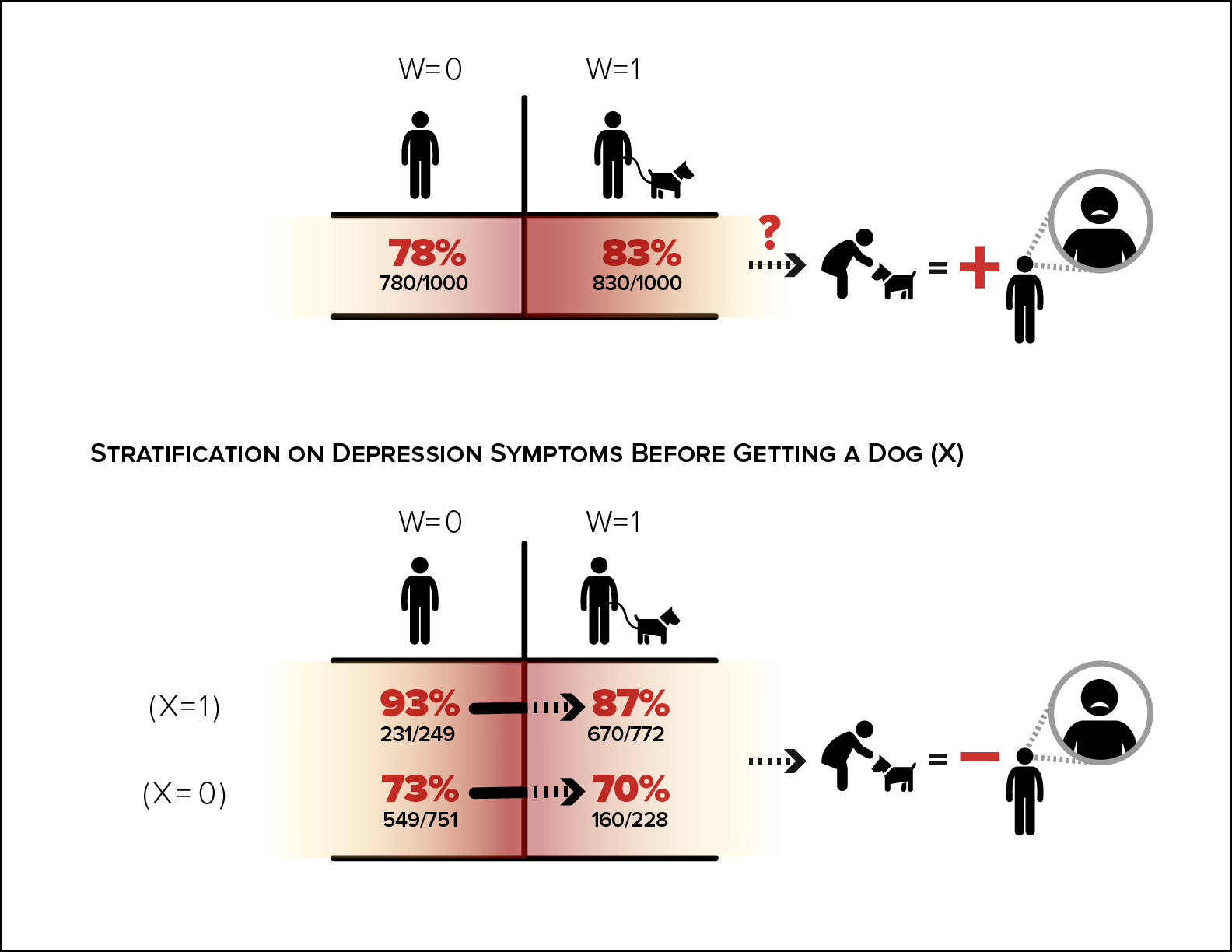
Figure 1. Top panel: rate of experiencing depression symptoms one year after getting a dog $W=1$ (83%) and one year after not getting a dog $W=0$ (78%). Bottom panel: rate of experiencing severe depression symptoms one year after getting a dog $W=1$ and one year after not getting the dog $W=0$, but separately for the two sub-populations that experienced severe or mild symptoms of depression before treatment assignment, denoted by $X=1$ and $X=0$, respectively. In the top panel, where we do not stratify by levels of $X$, getting a dog seems to increase the degree of severity of depression symptoms. In the bottom panel, where we stratify by levels of $X$, getting a dog appears to decrease the severity of depression symptoms.

Figure 1 provides an example of confounding. Let’s assume we compare two samples: one that adopts a dog $(W=1)$ and one that does not $(W=0)$. Then within each of these two populations, we calculate the rate of experiencing severe symptoms of depression $Y=1$. We found that adopting a dog appears to make the symptoms of depression worse: if you have a dog you are 5% more likely ($83\%$ versus $78\%$) to experience severe symptoms of depression. Should we advise people not to own dogs? The problem with this analysis is that we ignore the fact that the subjects might be different in ways that would bias the conclusions. As mentioned before, a key potential confounder is the degree of severity of their depression symptoms before they were assigned the treatment ($X$). For example, let’s stratify the two populations (treated and untreated) based on whether they experience severe or milder depression symptoms of ($X=1$ versus $X=0$) before treatment assignment. We find that within these two population strata, adopting a dog reduces the rate of experiencing severe symptoms of depression.

This is an example of what is known as Simpson’s paradox. Here the paradox occurs because people with severe depression symptoms before treatment assignment are more likely to adopt a dog. If we define by $e_{i}=P(W_{i}|X_{i})$ the propensity of adopting a dog conditional to the level of depression symptoms pre-treatment assignment, then in this example $P(W_{i}=1|X_{i}=1)=772/(772+249)$ is higher than $P(W_{i}=1|X_{i}=0)=228/(228+751)$. In other words, the assignment to treatment, who gets a dog and who does not, is not completely random, as in a RCT. It is influenced by the pre-existing level of depression of the study subjects. Situations like these are very common in observational studies. We argue that the potential outcome (PO) framework detailed below allows us to design an observational study and clarify the assumptions that are required to estimate the causal effects in these studies. Such assumptions translate expert knowledge into identifying conditions that are hard, if not impossible, to verify from data alone.

The PO framework is rooted in the statistical work on randomized experiments by Fisher, (1918, 1925) and Neyman, (1990), extended by Rubin, (1974, 1976, 1977, 1978, 1990) and subsequently by others to apply to observational studies. This perspective was called Rubin’s Causal Model by Holland, (1986) because it viewed causal inference as the result of missing data, and proposed explicit mathematical modeling of the assignment mechanism to reveal the observed data.

3. The Design Phase of a Study

We begin this section by describing the key distinctions between an RCT and an observational study. Table 1 summarizes and contrasts the main differences between RCTs and observational studies, and includes guidance on how to conduct causal inference in the context of observational studies in the last column.

The appeal of the RCT is that the design phase of the study (e.g. units, treatment, and timing of the assignment mechanism) is clearly defined a priori before data collection, including how to measure the outcome. In this sense, the RCT design is always prospective: treatment assignment randomization always occurs before the outcome is measured. A key feature of RCTs is that the probability of getting the treatment or the placebo, defined as the propensity score, is known – under the experimenter’s control – and it does not depend on unobserved characteristics of the study subjects. Randomization of treatment assignment is also fundamentally useful because it balances observed and unobserved covariates between the treated and control subjects. Once the design phase is concluded, the experimenter can proceed with the analysis phase, that is, estimating the causal effects based on a statistical analysis protocol that was pre-selected without looking at the information on the outcome. The separation between design and analysis is critical as it guarantees objective causal inference. In other words, it will prevent the experimenter from picking and choosing the estimation method that would lead to their preferred conclusion (Rubin et al.,, 2008).

In observational studies the treatment conditions and the timing of treatment assignment are observed after the data have been collected. The data are often collected for other purposes – not explicitly for the study. As a result the researcher does not control the treatment assignment mechanism. Moreover, the lack of randomization means there is no guarantee that covariates are balanced between treatment groups which could result in systematic differences between the treatment group and the control group. Traditionally, practitioners do not draw a clear distinction between the design and analysis phase when they analyze observational data. They estimate causal effects using regression models arbitrarily choosing covariates. This lacks the clear protocol of RCTs. To make objective causal inference from observational studies, we must address these challenges. Luckily, it is possible to achieve objective causal inferences from observational studies with careful design that approximates a hypothetical, randomized experiment. A carefully designed observational study can duplicate many appealing features of RCTs, and provide an objective inference on causal effects (Rubin,, 2007; Rubin et al.,, 2008; Hernán and Robins,, 2016). In the context of causal inference, the design of an observational study involves at least three steps (presented below). These steps should be followed by an analysis phase where the estimation approach is defined according to a pre-specified protocol as in the RCT. The three steps in the design phase are:

1. define experimental conditions and potential outcomes (subsection 3.1);

2. define causal effect of interest, including assumptions for identifiability (subsection 3.2);

3. construct a comparison group (subsection 3.3).

Table 1. Randomized Control Trials versus Observational Studies

	Randomized	Observational	Best practices for causal inference in
Study characteristics	Control Trials	Studies	observational studies
Basic concepts
Units	Defined before	Generally	Define units and treatments
Treatment	data are collected	not specified
Timing of treatment			Determine timing of treatment
assignment			assignment relative to measured
			variables
Design phase		The separation	Hide outcome data
versus	Separated	is unclear	until design phase
Analysis phase			is complete
Treatment assignment mechanism
Unconfounded	✓	?	Do data contain key confounders?
Probabilistic	✓	?	Yes: Assume unconfoundedness
Known	✓	?	No: Give up,
			find a better data source,
			or use a different identification strategy
Covariate balancing	Guaranteed	Not guaranteed	1. Assess overlap in covariates
			distribution
	(in expectation)		2. Remove units not similar to any
			units in the opposite treatment group
			3. Find subgroups in which the
			treatment groups are balanced on
			covariates
Type of analysis	By protocol	Regression	Analyze according to
			a pre-specified protocol
			Complement results with sensitivity analysis
			to deviations from assumptions

3.1. Define the experimental conditions and the potential outcomes

The first step to address a causal question is to identify the conditions (actions, treatments, or exposure levels) required to assess causality. To define the causal effect of $W=1$ versus $W=0$ on $Y$, one must postulate the existence of two potential outcomes: $Y(W=1)$ and $Y(W=0)$. As the name implies, both variables are potentially observable, but only the variable associated with the observed (or assigned) action will be observed. The critical feature of the notion of a cause is that the value of $W$ for each unit can be manipulated. To illustrate this idea, we now introduce the subscripts $(t-1)$ and $t$ to indicate time at or before the treatment assignment and time after treatment assignment (e.g., one year later). For example, let’s say Amy (subject $i$ at a specific time $t-1$) adopted a dog ($W_{i,t-1}=1$) and we observe her depression symptoms one year later $t$ ($Y_{i,t}(W_{i,t-1}=1)=Y_{i,t}(1)$). Now we must assume that $W$ can be manipulated, that is, we must be able to hypothesize a situation were Amy would not get a dog ($W_{i,t-1}=0$). So, $Y_{i,t}(1)$ is observed and $Y_{i,t}(0)$ is unobserved.

3.2. Define the causal effect of interest

We define a unit-level causal effect as the comparison between the potential outcome under treatment and the potential outcome under control. For example, the causal effect of $W$ on $Y$ for unit $i$ is defined as $Y_{i,t}(1)-Y_{i,t}(0)$.

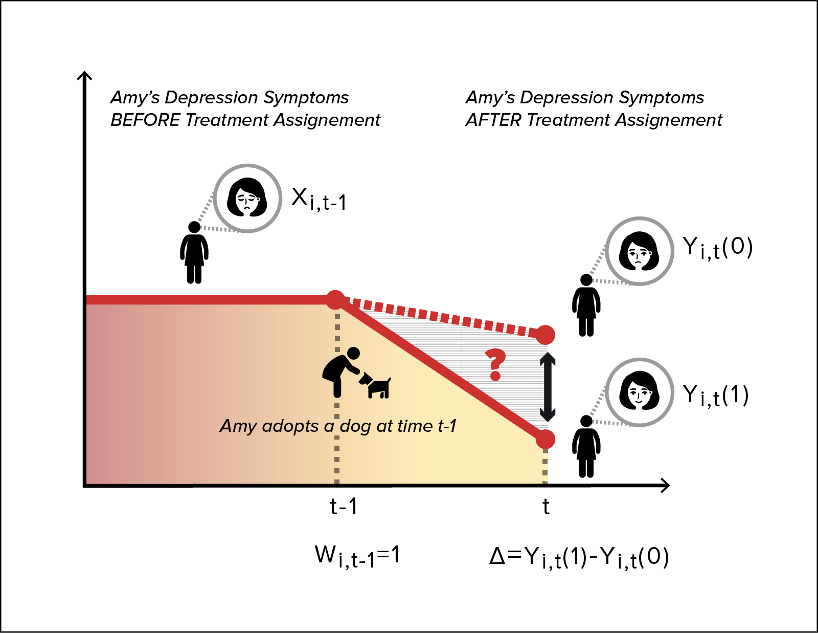
Figure 2. Causal effects as contrasts of potential outcomes at a given time point $t$.

As we can see from Figure 2, the causal effect of interest, is not a pre/post comparison of the depression symptoms for Amy (defined as $Y_{i,t}(1)-X_{i,t-1}$). It is, instead the difference between her two potential outcomes evaluated at time $t$, defined as $Y_{i,t}(1)-Y_{i,t}(0)$, where $Y_{i,t}(1)$ is observed, whereas $Y_{i,t}(0)$ is not. These differences are called individual treatment effects (ITE) (Rubin,, 2005).

While difficult to estimate (e.g., Funk et al.,, 2011), ITEs inform treatment effect heterogeneity (e.g., Dahabreh et al.,, 2016) and facilitate decision making in individualized settings where an estimate of the causal effect averaged across all the subjects in the sample may not be very practical (e.g., Li et al.,, 2019). We will return to this issue in Section 5. The last column of Table 2 introduces the concept of summarizing individual causal effects across the population of interest. For example, we can summarize the unit-level causal effects by taking the average difference, or by taking the difference in median values of the $Y_{i}(1)$s and $Y_{i}(0)$s, respectively. We typically focus on causal estimands that contrast potential outcomes on a common set of units (our target sample of size $N$), for example the average treatment effect (ATE): $\frac{1}{N}\sum_{i=1}^{N}(Y_{i}(1)-Y_{i}(0))=\bar{Y}(1)-\bar{Y}(0)$.

Table 2. The Science

Units	Covariates	Potential Outcomes	Potential Outcomes	Unit-level	Summary of
	$X$	$Y(1)$	$Y(0)$	Causal Effects	Causal Effects
1	$X_{1}$	$Y_{1}(1)$	$Y_{1}(0)$	$Y_{1}(1)$ vs $Y_{1}(0)$	Comparison of
.	.	.	.	.	$Y_{1}(1)$ vs $Y_{1}(0)$
$i$	$X_{i}$	$Y_{i}(1)$	$Y_{i}(0)$	$Y_{i}(1)$ vs $Y_{i}(0)$	for a common
.	.	.	.	.	set of units
N	$X_{N}$	$Y_{N}(1)$	$Y_{N}(0)$	$Y_{N}(1)$ vs $Y_{N}(0)$

The fundamental challenge is that we will never observe a potential outcome under a condition other than the one that actually occurred, so that we will never observe an individual causal effect (see Table 3). Holland, (1986) refers to this as the fundamental problem of causal inference. We typically refer to the missing potential outcome as the counterfactual and to the observed outcome as the factual outcome. Causal inference relies on the ability to predict the counterfactual outcome. It is important to note that methods used to predict or impute counterfactuals are different than off-the-shelf prediction or imputation often used for missing values. This is because we will never be able to find data where both potential outcomes $(Y_{i}(1),Y_{i}(0))$ are simultaneously observed on a common set of units. Table 3 highlights other fundamental implications of this representation of causal parameters: a) Uncertainty remains even if the $N$ units are our finite population of interest, because of the missingness in the potential outcomes; b) The inclusion of more units provides additional information (more factual outcomes) but also increases missingness (more counterfactual outcomes).

Data alone is not sufficient to predict the counterfactual outcome. We need to introduce several assumptions that essentially embed subject matter expert knowledge (Angrist and Pischke,, 2008). This is why machine learning alone cannot resolve causal inference problems, an issue discussed further in Section 5. To identify a causal effect from the observed data we have to make several assumptions.

Table 3. What we are able to observe about the Science

Units	Covariates	Treatment	Potential Outcomes		Unit-level
	$X$	$W$	$Y(1)$	$Y(0)$	Causal Effects
$1$	$X_{1}$	1	$Y_{1}(1)$	?	?
⋮	⋮	⋮	⋮	⋮	⋮
$i$	$X_{i}$	0	?	$Y_{i}(0)$	?
⋮	⋮	⋮	⋮	⋮	⋮
$N$	$X_{N}$	1	$Y_{N}(1)$	?	?

Assumption 1: Stable Unit Treatment Value Assumption (SUTVA). SUTVA, introduced and formalized in a series of papers by Rubin (see Rubin,, 1980, 1986, 1990), requires that there is no interference and no hidden version of the treatment. No interference assumes that the potential outcomes of a unit $i$ only depend on the treatment unit $i$ receives, and are not affected by the treatment received by other units.

For example epidemiological studies of the causal effects of non-pharmaceutical interventions (e.g., stay-at-home advisory) on the probability of getting COVID19 violate the assumption of no interference. This is because the individual level outcome (whether or not a subject is infected) depends on whether he/she complies with the stay-at-home advisory, but also on whether or not others in the same household also comply with the stay-at-home advisory.

Spillover effects are a violation of the no interference assumption. These examples often occur when the observations are correlated in time or space. In our ice cream case study this assumption is likely to hold as it is reasonable to assume that the only person who benefits from weight loss is the person that stopped eating ice cream. SUTVA violations can be particularly challenging in air pollution regulation studies as pollution moves through space and presents a setting for interference. Intervening at one location (e.g., a pollution source) likely affects pollution and health across many locations, meaning that potential outcomes at a given location are probably functions of local interventions as well as interventions at other locations (Papadogeorgou et al.,, 2019; Forastiere et al.,, 2020). The condition of no hidden version of treatments requires that potential outcomes not be affected by how unit $i$ received treatment. This assumption is related to the notion of consistency (Hernán,, 2016; Hernán and Robins,, 2020). For example, how Amy adopted a dog (a friend giving away puppies or driving to a breeder) does not affect Amy’s outcome.

Our ability to estimate the missing potential outcomes depends on the treatment assignment mechanism. That, is, it depends upon the probabilistic rule $W=1$ versus $W=0$ which determines whether $Y(1)$ or $Y(0)$ is observed. The assignment mechanism is defined as the probability of getting the treatment conditional on $X,Y(1),Y(0)$, e.g. $P(W|X,Y(1),Y(0))$. This expression will be simplified under the next assumption.

Assumption 2: No unmeasured confounding. The assignment mechanism is unconfounded if: $P(W\mid X,Y(1),Y(0))=P(W\mid X)$. Unconfoundedness is also known as no unmeasured confounding assumption, or conditional independence assumption. This means that if we can stratify the populations within subgroups that have the same covariate values (e.g., same age, gender, race, income), then within each of these strata, the treatment assignment (e.g., who gets the drug and who does not) is random.

The assumption allows to provide a formal definition of a confounder. Although there is no consensus regarding a unique and formal definition, we adopt the one proposed by VanderWeele and Shpitser, (2013): a pre-exposure covariate $X$ is said to be a confounder for the effect of $W$ on $Y$ if there exists a set of covariates $X^{*}$ such that the effect of $W$ on $Y$ is unconfounded conditional on $(X^{*},X)$, but it is not for a subset of $(X^{*},X)$. Equivalently, a confounder is a member of a minimally sufficient adjustment set.

Unconfoundedness is critical to estimate causal effects in observational studies. As $Y_{i}(1)$ is never observed on subjects with $W_{i}=0$ and $Y_{i}(0)$ is never observed on subjects with $W_{i}=1$, we cannot test this assumption, and so its plausibility relies on subject-matter knowledge. As a result, sensitivity analysis should be conducted routinely to assess how the conclusions will change under specific deviations from this assumption (discussed in Section 6). Moreover, this assumption may fail to hold if some relevant covariates are not observed, or if decisions are based on information on potential outcomes. For example a perfect doctor (Imbens and Rubin,, 2015) gives a drug to patients based on who benefits from the treatment (e.g., $W_{i}=I(Y_{i}(1)>Y_{i}(0))$): the assignment is confounded – i.e. depends on the potential outcomes, irrespective of the covariates we are able to condition on. We discuss these situations in our final remarks.

Assumption 3: Overlap or positivity. We define the propensity score for subject $i$ as the probability of getting the treatment given the covariates (Rosenbaum and Rubin,, 1983) $e_{i}=P(W_{i}=1\mid X_{i})$. The assumption of overlap requires that all units have a propensity score that is between 0 and 1, that is, they all have a positive chance of receiving one of the two levels of the treatment.

In the depression/dog example, this may be violated if some people in the population of interest are allergic to dogs and therefore their probability of getting a dog is zero. In the clinical example, this hypothesis is commonly violated if a patient has a genetic mutation that prevents him/her from receiving the treatment being tested. Because the propensity score can be estimated from data, we can check if overlap holds. If for some units the estimated $e_{i}$ is very close to either $1$ or $0$, then these units are only observed under a single experimental condition and therefore contain very little information about the causal effect. In this situation, strong assumptions are necessary. For example, a strong assumption is to say that the functional form that relates the covariates with the outcome holds also outside of the observed range of the covariates. A more formal approach of how to overcome violations of the positivity assumption is presented in Nethery et al., (2019). If assumptions 2 and 3 are both met, then we conclude that the assignment mechanism is strongly ignorable (Rosenbaum and Rubin,, 1983). Classic randomized experiments are special cases of strongly ignorable assignment mechanisms.

3.3. How to construct an adequate comparison group

Once you have identified relevant potential confounders, and assuming they are sufficient for unconfoundedness to hold, the issue of confounding can be resolved by constructing an adequate comparison group. This is a crucial step in the design of an observational study. Our goal is to synthetically recreate a setting that is very similar to a randomized experiment, so the joint distribution of all the potential confounders is as similar as possible between the treatment and control groups (Ho et al.,, 2007; Stuart and Rubin,, 2008; Stuart,, 2010). For instance, let’s return to our example about Amy (in this case we drop the subscript $t$). Amy (subject $i$) got a dog $W_{i}=1$, so we observe $Y_{i,obs}=Y_{i}(W_{i}=1)$ whereas $Y_{i,mis}=Y_{i}(W_{i}=0)$. To estimate a causal effect we need to predict $Y_{i}(W_{i}=0)$, that is, what we would expect the severity of Amy’s symptoms to be under the hypothetical (not observed) scenario in which Amy did not get the dog ($W_{i}=0$). To predict the missing counterfactual $Y_{i}(W_{i}=0)$, we need to define an adequate control group. Based on the considerations made so far, we need to find subjects that are similar to Amy with respect to the potential confounders (age, race, income, health status, severity of depression symptoms) before treatment assignment. The only difference between the matched subjects and Amy is that they did not get a dog. This should be done for Amy and for any subject in our target population who got a dog. With a large number of confounders matching on all confounders exactly may not be feasible. A common approach to address this challenge is to use propensity scores ($e_{i}$) and match subjects with respect to $e_{i}$. The estimated propensity score is an univariate summary of all covariates and is crucial to estimate causal effects under unconfoundedness (Robins et al.,, 1995; Robins and Rotnitzky,, 1995; Imbens and Rubin,, 2015; Imai and Ratkovic,, 2014). Subjects sharing the same value of the propensity score have the same distribution of the observed potential confounders whether they are treated or not. Estimated propensity scores can be applied in the design phase to assess overlap and construct a comparison group through matching, stratifying, or weighting observations (Rubin et al.,, 2008). Covariate balance can also be viewed as an optimization problem. Procedures based on this idea either directly optimize weights or find optimal subsets of controls such that the mean or other characteristics of the covariates is the same in the treatment and control group (Zubizarreta,, 2012; Diamond and Sekhon,, 2013; Zubizarreta et al., 2014a, ; Zubizarreta,, 2015; Li et al.,, 2018; Li and Thomas,, 2018).

To this point we have only discussed what we are interested in estimating, the study design, and the problem of confounding. Now we will discuss how we estimate the causal effects. Being able to identify causal effects is a feature of the causal reasoning used in the potential outcome framework. Without including causal reasoning in the design phase you cannot to recover the causal effect even with the most sophisticated machine learning or nonparametric methods (e.g., Mattei and Mealli,, 2015).

4. Estimation

Causal estimands such as $ATE=\overline{Y}(1)-\overline{Y}(0)$ are a function of the observed $Y_{obs}$ and the missing potential outcomes (the counterfactuals) $Y_{mis}$. Therefore, an estimation strategy needs to implicitly or explicitly impute $Y_{mis}$. What follows is not a comprehensive review of all estimation methods of causal effects, but rather key ideas of Bayesian estimation of the average treatment effect (Rubin,, 1978; Imbens and Rubin,, 2015; Ding and Li,, 2018).

4.1. Bayesian methods for the imputation of the missing counterfactuals after the design phase is concluded

Within the model-based Bayesian framework for causal inference (Rubin,, 1975, 1978), the $Y_{mis}$ are considered unknown parameters. The goal is to sample from their posterior predictive distribution conditionally to the observed data defined as:

$$P(Y_{mis}|Y_{obs},X,W)\propto P(X,Y(1),Y(0))P(W|X,Y(1),Y(0))$$ (1)

where $P(X,Y(1),Y(0))$ denotes the model for the potential outcomes, while $P(W|X,Y(1),Y(0))$ denotes the model for the treatment assignment. By sampling from this posterior distribution we can multiply impute $Y_{mis}$, and then estimate $ATE$, or any other causal contrast, and its posterior credible interval (Rubin,, 1978; Mealli et al.,, 2011). Note that this missing data imputation exercise is critically different from a usual prediction task: the two models introduced above contain expert knowledge (for example the assumption of strong ignorability or the inclusion of relevant covariates) that cannot be retrieved from data alone. Under unconfoundedness or no unmeasured confounding (Assumption 2: $P(W|X,Y(1),Y(0))=P(W|X)$), and assuming the parameters of the model for the potential outcomes are a priori independent of the parameters of the model for the assignment mechanism, then the posterior distribution of the missing potential outcomes only depends on the parameters of the model for the outcomes. Specifically, assuming exchangeability (de Finetti,, 1963), there exists a parameter vector $\theta$ having a known prior distribution $p(\theta)$ such that:

$$P(Y(0),Y(1),W,X) = \int\prod_{i}P(Y_{i}(0),Y_{i}(1),W_{i},X_{i},\theta)p(\theta)~{}d\theta.$$ (2)

The posterior predictive distribution of the missing data, $P(Y_{mis}\mid Y_{obs},W,X)$, can be written as

$$P(Y_{mis}\mid Y_{obs},W,X)$$

$$= \frac{P(Y(0),Y(1),W,X)}{\int P(Y(0),Y(1),W,X)dY_{mis}}$$

$$= \frac{\int\prod_{i}P(W_{i}\mid Y_{i}(0),Y_{i}(1),X_{i},\theta)P(Y_{i}(0),Y_{i}(1)\mid X_{i},\theta)P(X_{i}\mid\theta)p(\theta)d\theta}{\int\!\!\int\prod_{i}P(W_{i}\mid Y_{i}(0),Y_{i}(1),X_{i},\theta)P(Y_{i}(0),Y_{i}(1)\mid X_{i},\theta)P(X_{i}\mid\theta)p(\theta)~{}d\theta dY_{mis}}.$$

Let $\theta_{W|X}$, $\theta_{Y|X}$ and $\theta_{X}$, denote the unknown parameters corresponding to the distribution of the treatment assignment mechanism (e.g. the propensity score), the distribution of potential outcomes, and the distribution of covariates, respectively. Then, given ignorability, the propensity score $P(W_{i}\mid X_{i},\theta_{W|X})$ and the covariates’ distribution $P(X_{i}\mid\theta_{X})$ cancel out in Equation (4.1), which simplifies to:

$$P(Y_{mis}\mid Y_{obs},W,X) \propto \int\prod_{i}P(Y_{i}(0),Y_{i}(1)\mid X_{i},\theta_{Y|X})p(\theta_{Y|X})d\theta_{Y|X}$$ (4)

Equation (4) shows that, under ignorable treatment assignments, the potential outcome model needs to be specified $P(Y_{i}(w)\mid X_{i},\theta_{Y|X})$ for $w=0,1$, as well as the prior distribution $p(\theta_{Y|X})$, to derive the posterior distribution of the causal effects. Therefore, the most straightforward Bayesian approach to estimate causal effects under ignorability is to specify models for $Y(1)$ and $Y(0)$ that are conditional to covariates and some parameters and then draw the missing potential outcomes from their posterior predictive distribution, which will also derive the posterior distribution of any causal estimand.

As such, it seems like propensity scores, that are central to balance the covariates in the design stage, do not affect Bayesian inference for causal effects under ignorability. However, as noted by Rubin, (1985), for effective calibration of Bayesian inference of causal effects (i.e., good frequentist properties) good covariate balance is necessary (Ding and Li,, 2019, see also). That is, if covariates are balanced between treatment groups, inference on causal effects derived from the estimation of the outcome model are robust and not very sensitive to model assumptions. Flexible semi- and non-parametric specifications of the outcome model can be found in literature including Bayesian Additive Regression Models (BART; Hill,, 2011; Hahn et al.,, 2020) or Bayesian Cubic Splines (Chib and Greenberg,, 2010).

4.2. Bayesian methods for joint estimation of the outcome and propensity score models and the feedback problem

Some Bayesian methods explicitly include the estimation of the propensity score in the causal effects’ estimation procedure. Some of these approaches involve the specification of a regression model for the outcome with the propensity score as a single regressor, arguing that this modelling task is simpler than specifying a model for the outcome conditional on the whole set of (high-dimensional) covariates (Rubin,, 1985). This approach can be improved by adjusting for the residual covariance between $X$ and $Y$ at each value of $e(X)$ (Gutman and Rubin,, 2015), or by specifying an outcome model conditional on the covariates $X$ and the propensity score (Zheng and Little,, 2005).

These are two-stage methods that separate design (estimation of the propensity score) from analysis. Some authors have proposed a single step Bayesian approach to merge the two stages. For example, McCandless et al., (2009) proposed a joint modelling approach to estimate the outcomes and the propensity score in this setting. However Zigler et al., (2013) has shown that merging the two steps may induce the “feedback problem” if the parameters of the two models are a priori dependent. In this instance, the outcome information enters the estimation of the propensity score, contradicting ignorability, and can lead to a distorted estimate of the propensity scores and compromise estimates of causal effects. Consequently, these types of Bayesian models are not often used. Liao and Zigler, (2018) considers how uncertainty associated with the design stage impacts estimation of causal effects in the analysis stage. Uncertainty in the design stage may stem from the propensity score estimation but also from how the propensity score is used. Liao and Zigler propose a procedure that obtains the posterior distribution of causal effects after marginalizing distributed over design-stage outputs.

4.3. Bayesian methods to overcome violations of the positivity

To address violations of the positivity assumption Bayesian methods, including BART and splines, have also been developed. For example, Nethery et al., (2019) have recently developed a novel Bayesian framework to estimate population average causal effects with minor model dependence and appropriately large uncertainties in the presence of non-overlap. In this approach, the tasks of estimating causal effects in the overlap and non-overlap regions are delegated to two distinct models, suited to the degree of data in each region. In this case, tree ensembles are used to non-parametrically estimate individual causal effects in the overlap region, where the data can speak for themselves. In the non-overlap region, where insufficient data support makes reliance on model specification necessary, individual causal effects are estimated by extrapolating trends from the overlap region via a spline model. The authors showed that their proposed approach has a good performance compared to approaches that perform estimation only in the area of overlap (Hill and Su,, 2013; Zigler and Cefalu,, 2017).

4.4. Bayesian and non-Bayesian methods that are model-free

Estimation methods under ignorability that are model-free (i.e., matching, stratification, weighting) are usually frequentist and treat potential outcomes as fixed values instead of random variables Imbens and Rubin, (2015); Imbens, (2004); Yao et al., (2020). Some authors have proposed quasi-Bayesian approaches that involve only the Bayesian estimation of the propensity score, and then estimate the causal effect via matching (An,, 2010), stratification or weighting (Saarela et al.,, 2015). These approaches are not fully Bayesian in that they incorporate only the uncertainty in the propensity score estimation and not in the imputation of the missing potential outcomes. The frequentist methods have been improved by combining them with outcome regression adjustments (e.g., Abadie and Imbens,, 2011). Robins and colleagues (e.g., Scharfstein et al.,, 1999; Robins,, 2000; Lunceford and Davidian,, 2004; Bang and Robins,, 2005; Robins and Rotnitzky,, 1995; Robins et al.,, 1995; Funk et al.,, 2011; Knaus,, 2020) have proposed a class of double robust (DR) estimators that combine inverse probability weighting estimator (IPW) with an outcome regression. Interestingly, Gustafson, (2012) casted DR estimator from a Bayesian perspective as a weighted average of a parametric model and a satured model for the outcome conditional on covariates, with weights that depend on how well the parametric model fits the data. As a result, it can also be viewed as a Bayesian model average estimator (Cefalu et al.,, 2016).

4.5. Bayesian and non-Bayesian methods to account for variable selection either in the propensity or in the outcome model

Zigler and Dominici, (2014) proposed a Bayesian model averaging method to adjust for the uncertainty in the selection of the covariates in the propensity score model, extending Wang et al., (2012); see also Wang et al., (2015). When the number of the potential confounders is larger than the number of observations, approaches for dimension reduction and penalization are required. The standard approaches (e.g., the Lasso) generally aim to predict the outcome, and are less suited for estimation of causal effects. Under standard penalization approaches, if a variable $X$ is strongly associated with the treatment $W$ but weakly associated with the outcome $Y$, its coefficient will be reduced towards zero leading to confounding bias. Belloni et al., 2014b ; Belloni et al., 2014a proposed a modified version of Lasso, called double Lasso, to reduce confounding bias. There are several Bayesian alternatives that usually outperform such approaches, for example using continuous spike and slab priors on the covariates’ coefficients in the outcome and propensity score models (Wang et al.,, 2015; Cefalu et al.,, 2016; Antonelli et al.,, 2017; Antonelli and Dominici,, 2018).

5. The perils and the strengths of machine learning methods in causal inference

We have presented approaches for the estimation of $Y_{mis}$ with high dimensional covariates and nonparametric methods, and the related issue of variable selection. At first glance, these tasks could be addressed by implementing off-the-shelf machine learning methods, but there are challenges. In this section we provide critical insights regarding the application of machine learning methods in causal inference.

Machine learning methods primarily address prediction or classification problems, and have been included in statistical textbooks (e.g., Hastie et al.,, 2009; James et al.,, 2013; Efron and Hastie,, 2016). On a high level, there are two broad categories of machine learning methods: supervised and unsupervised learning. In supervised learning, the predictors (i.e. covariates, features) $X$ and the outcome $Y$ are both observed. The goal is to estimate the conditional mean of an outcome $Y$ given a set of covariates or features $X$, to ultimately predict $Y$. These methods include decision trees (e.g. Breiman et al.,, 1984), random forests (Breiman,, 2001), gradient boosting (Friedman,, 2001), support vector machines (Cortes and Vapnik,, 1995; Suykens and Vandewalle,, 1999), deep neural networks (e.g., LeCun et al.,, 2015; Farrell et al.,, 2018), ensemble methods (e.g., Dietterich,, 2000), and variable selection tools such as LASSO (Tibshirani,, 1996; Hastie et al.,, 2015). Regression trees, and random forests as their extension, have become very popular methods for estimating regression functions in settings where out-of-sample predictive power is important. When the outcome $Y$ is an unordered discrete response, these supervised learning algorithms attempt to resolve classification problems - for example detecting spam emails. In this instance, a machine learning algorithm is trained with a set of spam-emails labelled as spam and not-spam emails labelled as not-spam, so that a new email can be classified as either spam or not-spam. In unsupervised learning (see Hastie et al.,, 2009) only features $X$ are observed and the goal is to group observations into clusters (Jain et al.,, 1999). Clustering algorithms essentially group units based on their mathematical similarities and dissimilarities of features $X$. These tools can be used for example to find groups of basketball or soccer players with similar attributes and then interpret and use these clusters to form teams or to target coaching. Deep learning methods are another general and flexible approach to estimate regression functions. They perform very well in settings with extremely large number of features, like image recognition or image diagnostics (He et al.,, 2016; Simonyan and Zisserman,, 2014). These methods typically require a large amount of tuning to work well in practice, relative to other methods such as random forests, and as a result we will not discuss them further in this article.

Since machine learning supervised learning methods aim to estimate the conditional mean of an outcome $Y$ given $X$ it would on the surface appear to be a good fit to exploit machine learning methods to estimate the missing potential outcomes and as a result the causal effects, especially in high-dimensional settings. However, it is not that simple. The following section presents the circumstances under which off-the-shelf supervised learning machine learning methods might not be appropriate with regard to causal inference. We also discuss how these methods can be adapted to achieve estimation of causal effects; how machine learning and the literature on statistical causal inference can cross-fertilize; and the open questions and problems that machine learning cannot handle on its own.

5.1. Why off-the shelf machine learning techniques might not be appropriate for causal inference.

A key distinction between causal inference and machine learning is that the former focuses on estimation of the missing potential outcomes, average treatment effects, and other causal estimands, and machine learning focuses on prediction and classification. Therefore machine learning dismisses covariates with limited prediction importance. However, in causal inference if these same covariates are correlated with the treatment assignment they can be important confounders. As previously discussed omitting covariates from the analysis that are highly correlated with the treatment can introduce substantial bias in the estimation of the causal effects even if their predicting power is weak. Another major difference is that machine learning methods are typically assessed on their out-of-sample predictive power. This approach has two major drawbacks in the context of causal inference. First, as pointed out by Athey and Imbens, (2016), a fundamental difference between a prediction and the estimation of a causal effect is that in causal inference we can never observe the ground truth (e.g., in this context the counterfactual). That is, in our example, because Amy has adopted a dog, we will never be able to measure the severity of the Amy’s depression symptoms under the alternative hypothetical scenario where Amy did not adopt a dog. Therefore, standard approaches for quantifying the performance of machine learning algorithms cannot be implemented to assess the quality of prediction of the missing potential outcomes and therefore the causal effects (Gao et al.,, 2020). Second, in causal inference we must provide valid confidence intervals for the causal estimands of interest. This is required to make decisions regarding which treatment or treatment regime is best for a given unit or subset of units, and whether a treatment is worth implementing. Another limitation of machine learning techniques in causal inference is that they are developed for the most part in settings where the observations are independent and therefore have limited ability to handle data that is correlated in time and/or in space, such as time series, panel data, spatially correlated processes. Additionally, they are not able to handle specific structural restrictions suggested by subject-matter knowledge, such as monotonicity, exclusion restrictions, and endogeneity of some variables (Angrist and Pischke,, 2008; Athey and Imbens,, 2019).

5.2. How machine learning methods can adapt to the goal of estimation of causal effects.

Machine learning methods have been adapted to address causal inference. One popular approach is to redefine the optimization criteria, which typically depend on a function of the prediction errors, to prioritize issues arising in causal inference, such as the controlling for confounders and the discovering of treatment effect heterogeneity (Chernozhukov et al.,, 2017, 2018). For example, the causal tree method proposed by Athey and Imbens, (2016) is based on a rework of the criterion function of Classification and Regression Trees (Breiman et al.,, 1984) – originally aimed at minimising the predictive error – to maximise the variation in the treatment effects and, in turn, discover the subgroups with the highest heterogeneity in the causal effects (further details are presented in Section 6). Typical regularizing algorithms used in machine learning, such as Lasso, Elastic Net and Ridge (Hastie et al.,, 2015), must prioritize confounding adjustment to avoid missing relevant covariates, as seen in Belloni et al., 2014b and Belloni et al., 2014a and discussed in Section 4.5. Additional research efforts are required to study the statistical properties of machine learning techniques, as in Wager and Athey, (2018) and Athey et al., (2019) for random forests and Jeong and Rockova, (2020) for BART. Treatment effect estimators based on causal random forests have been shown to be point-wise consistent and asymptotically normal, while estimators based on BART are asymptotically optimal. Both these asymptotic results hold true under a set of specific conditions that are not necessarily mild. However, research has shown that machine learning algorithms show promise when the hardest issues are resolved during design (Dorie et al.,, 2019; Hahn et al.,, 2019; Bargagli-Stoffi et al.,, 2019; Knaus et al.,, 2020; Bargagli-Stoffi and Gnecco,, 2020). Specifically, it is critical to first identify a good control population, for example using propensity score matching as discussed earlier. After we have achieved this critically important task, then we can be confident that the assumptions of identifiability of causal effects are met. Only at this stage, the machine learning techniques provides an excellent tool to predict the missing counterfactuals (e.g., Chernozhukov et al.,, 2018). However, it is important to keep in mind that performance will ultimately rely on the flexible parametrization that machine learning methods impose on the data, the plausibility of the unconfoundedness assumption, and the extent of the overlap in the distribution of the covariates (Hernán et al.,, 2019). Even in the presence of a high-dimensional set of covariates, the study design is important (D’Amour et al.,, 2017).

5.3. Cross-fertilization between machine learning and causal inference problems

Several machine learning techniques have been adapted to improve traditional causal inference methods. These include approaches to regularization (the process of adding information to solve ill-posed problems or to prevent overfitting) that scale well to large datasets (Chang et al.,, 2018) and the related concept of sparsity (the idea that some variables may be dropped from the analysis without affecting the performance of estimation of causal effects). The use of model averaging and ensemble methods common in machine learning is a practice that is now exploited in causal inference (see Section 4) (Van der Laan and Rose,, 2011; Cefalu et al.,, 2016).

Framing data analysis as an optimization problem has inspired the development of causal inference methods based on direct covariate balancing. For example, Zubizarreta, (2015) which optimizes weights for each observation instead of trying to estimate the propensity score so that the covariate distribution is the same in the treatment and control group. Matrix completion methods were originally developed in machine learning for the imputation of the missing entries of a partially observed matrix (Candès and Recht,, 2009; Recht,, 2011). These methodologies can be used to improve causal inference methods for panel data and synthetic control methods (Abadie et al.,, 2010) in settings with large $N$ and $T$. In particular, matrix completion can be successfully adapted for the imputation of missing counterfactuals when a large proportion of potential outcomes is missing (Athey et al.,, 2018).

5.4. Open questions and problems that machine learning alone cannot handle.

However, even when adapted to treatment effect estimation, machine learning algorithms must be implemented with extreme caution when there are unresolved key issues surrounding the study design. For example:

• The sample under study is not representative of the population about which we need or want to draw conclusions;

• The number of potential confounders that are measured may not be sufficient: there is nothing in the data that tells us that unconfoundedness holds; causal effect estimation should be followed by a well-designed sensitivity analysis;

• The presence of post-treatment variables that must be excluded (i.e., variables that can be affected by the treatment and are strong predictor of the outcome);

• The lack of overlap (Nethery et al.,, 2019; D’Amour et al.,, 2017) in the distribution of the estimated propensity scores for the treated and untreated, demands the machine extrapolate beyond what is observed;

• If interference is detected, causal estimands (direct and indirect - spillover - effects) need to be re-defined and different estimation strategies need to be implemented. (Arpino and Mattei,, 2016; Forastiere et al.,, 2016; Papadogeorgou et al.,, 2019; Bargagli-Stoffi et al.,, 2020; Tortú et al.,, 2020).

Even in settings where machine learning can accurately predict potential outcomes (Wager and Athey,, 2018; Hahn et al.,, 2020; Belloni et al., 2014a, ; Chernozhukov et al.,, 2017, 2018), they cannot handle other problems such as missing outcomes (Hill,, 2004; Mattei et al.,, 2014), (non-random) measurement error or misclassification of outcome or treatment (Imai and Yamamoto,, 2010; Pierce and VanderWeele,, 2012; Funk and Landi,, 2014), censoring due to death of the outcome (Rubin,, 2006; Mattei and Mealli,, 2007), and disentangling different causal mechanisms (Mattei and Mealli,, 2011; VanderWeele,, 2015; Baccini et al.,, 2017; Forastiere et al.,, 2018).

6. Treatment effect heterogeneity: is the treatment beneficial to everyone?

Suppose we found statistically significant evidence that a new drug prolonged life expectancy on average for the population under study. Should we encourage anyone, regardless of their age, income, or other diseases to take this new drug? It is often highly desirable to characterize which subgroups of the population would benefit the most or the least from a treatment. These types of questions require us to analyze treatment effect heterogeneity based on pre-treatment variables. There is extensive literature on assessing heterogeneity of causal effects that is based on estimating the conditional average treatment effect (CATE), which is defined as $E[Y(W=1)\mid X=x]-E(Y(W=0)\mid X=x]$ where $Y(W=1)\mid X=x$ and $Y(W=0)\mid X=x$ are the potential outcomes in the subgroups of the population defined by $X=x$. Conditionally to $X=x$, the CATE can be estimated with the same set of the causal assumptions that are needed for estimating the ATE (Athey and Imbens,, 2016). Recently, machine learning methods such as random forests, Bayesian Additive Regression Tree (BART) (Chipman et al.,, 2010), and forest based algorithms Foster et al., (2011) and Hill, (2011), have been used to estimate CATE, especially in the presence of high dimensional $X$. Despite accurately estimating the CATE using machine learning methods, these methods offer little guidance about which population subgroups are important in the treatment effect heterogeneity. Their parametrization of the covariate space is complicated and difficult to interpret even by human experts. We define interpretability as the degree to which a human can understand the cause of a decision or consistently predict the results of the model (Miller,, 2019; Kim et al.,, 2016). Decision rules fit well with this non-mathematical definition of interpretability. A decision rule consists of a set of conditions about the covariates, that define a subset of the features space, and correspond to a specific subgroup. In our recent work (Lee et al.,, 2020), we propose a novel causal rule ensemble (CRE) method that ensures interpretability of the causal rules while maintaining a high level of accuracy of the estimated treatment effects for each rule. We argue that in the context of treatment effect heterogeneity, we want to achieve at least two main goals: to (1) discover de novo the rules (that is, interpretable population subgroups) that lead to heterogeneity of causal effects, and (2) make valid inference about the CATE with respect to the newly discovered rules. Athey and Imbens, (2016) has introduced a clever approach to make valid inferences in this context. They introduced the idea of a sample-splitting approach that divides the total sample into two smaller samples: (1) to discover a set of interpretable decision rules that could lead to treatment effect heterogeneity (i.e. discovery sample), and (2) to estimate the rule-specific treatment effects and associated statistical uncertainty (i.e. inference sample). This is a very active area of research and one where the integration of machine learning and causal inference could provide important advances.

7. Sensitivity analysis

Sensitivity analyses can be conducted to bound the magnitude of the causal effects as a function of the degree to which the assumptions are violated to evaluate the robustness of causal conclusions to violations of unverifiable assumptions (Imbens and Rubin,, 2015; Ding and VanderWeele,, 2016). Sensitivity analysis is different from model assessment or model diagnostic, because identifying assumptions, such as unconfoundedness, are intrinsically untestable: the observed data are uninformative about the distribution of $Y(0)$ for treated units $(W=1)$ and about the distribution of $Y(1)$ for control units $(W=0)$. We like to argue that the larger the set of measured covariates the smaller the chance of unmeasured confounding bias, and it is thus often sensible to assume unconfoundedness. However, in practice, even if we have adjusted for all measured covariates, we can never rule out the possibility of an unmeasured confounder. A sensitivity analysis assumes the existence of at least one unmeasured confounder and posits assumptions on how it may relate to both treatment assignment and outcome. It then examines how the estimated causal effect varies as the degree of confounding bias, resulting from this unmeasured covariate, increases. Different strategies for sensitivity analysis have been proposed in the literature and include Rosenbaum, 1987b ; Rosenbaum, (2002); Imbens, (2003); Ichino et al., (2008); Gustafson et al., (2010); Liu et al., (2013); Ding and VanderWeele, (2016); VanderWeele and Ding, (2017); Franks et al., (2019); Zhang and Tchetgen, (2019). Software has been developed to perform sensitivity analyses that assesses the strength of conclusions to violations of unverifiable assumptions (Gang,, 2004; Nannicini,, 2007; Keele,, 2014; Ridgeway et al.,, 2004).

One type of sensitivity analysis is so-called placebo or negative control (Imbens and Rubin,, 2015). Here the goal is to identify a variable that cannot be affected by the treatment. This variable is then used as an outcome (say $Y^{\star}$) and the causal effect of $W$ on $Y^{\star}$ is estimated, when we know that the true causal effect, say $\Delta$, should be zero. If we estimate that $\Delta$ is statistically significantly different from zero, when we have adjusted for all the measured confounders, then we can conclude that there is unmeasured confounding bias. For additional details see Schuemie et al., (2020).

Sometimes we can check the quality of an observational control group by exploiting useful comparisons. For example, we can have access to two different pools of controls and use them both to check robustness of results to the use of either one (Rosenbaum, 1987a, ). We can also assess the plausibility of unconfoundedness and the performance of methods for causal effects in observational studies by checking the extent to which we can reproduce experimental findings using observational data. For example, Dehejia and Wahba, (2002) use data from LaLonde, (1986) evaluation of non-experimental methods that combine the treated units from a randomized evaluation of the National Supported Work (NSW) Demonstration, a labor training program, with non-experimental comparison units drawn from survey datasets. They show that estimates obtained with propensity score based estimators of the treatment effect are closer to the experimental benchmark estimate than other methods.

In addition to the challenge of adjusting for confounding bias, there is another key challenge that is often overlooked, and that is due to over adjustment. For example, controlling for post-treatment variables (such as mediators) will bias the estimation of the causal effects see for example Greenland et al., (1999); Hernán et al., (2004); Rubin et al., (2008); Shrier, (2008); Schisterman et al., (2009); Ding and Miratrix, (2015). In addition, it is common to include as many covariates as possible to control for confounding bias; however M-bias is a problem that may arise when the correct estimation of treatment effects requires that certain variables are not adjusted for (i.e., are simply neglected from inclusion in the model). The topic of over adjustment is also broadly discussed in the causal graphical models literature (see Pearl,, 1995; Shpitser et al.,, 2010; VanderWeele and Shpitser,, 2011; Perkovic et al.,, 2017).

8. Discussion

This article has focused on the potential outcome framework as one of the many approaches to define and estimate the causal effects of a given intervention on a outcome. We have presented:

• Thoughts regarding the central role of the study design when estimating causal effects (Table 1).

• Why machine learning is not a substitute for a thoughtful study design, and that it cannot overcome data quality, missing confounders, interference, or extrapolation.

• That machine learning algorithms can be very useful to estimate missing potential outcomes after issues related to study design have been resolved.

• Machine learning algorithms show great promises in discovering de novo subpopulations with heterogeneous causal effects.

• The importance of sensitivity analysis to assess how the conclusions are affected by deviations from identifying assumptions.

This review is focused on data science methods for prospective causal questions, that is, on assessing the causal effect of a particular, sometimes hypothetical, manipulation.

This is a different goal than that of causal discovery which investigates the causal structure in the data, without starting with a specified causal model. To read more about causal discovery we refer to Glymour et al., (2014); Mooij et al., (2016); Spirtes and Zhang, (2016).

We briefly outlined the Bayesian approach as one of the many statistical methods to estimate missing potential outcomes and the ATE. Alternative approaches such as those proposed by Fisher and Neyman are based on the randomization distribution of statistics induced by a classical randomized assignment mechanism (Neyman,, 1990; Fisher,, 1937) and their sampling distribution. The key feature of these approaches is that potential outcomes are treated as fixed but unknown, while the vector of treatment assignments, $W$, and the sampling indicators are the random variables. The concepts created by these methods, p-values, significance levels, unbiased estimation, confidence coverage, remain fundamental today (Rubin,, 2010). However, we believe that the Bayesian thinking provides a straightforward approach to summarize the current state of knowledge in complex situations, to make informed decisions about which interventions look most promising for future application and to properly quantify uncertainty around such decisions.

There are settings or instances where adjusting for measured covariates is not enough, that is, we cannot rule out dependence of the assignment mechanisms on the potential outcomes. In these irregular settings, another important area of research is relying on identification strategies that differ from strong ignorability, some of which are called quasi-experimental approaches. A natural experiment can be thought of as an observational study where treatment assignment, though not randomized, seems to resemble random assignment in that it is haphazard, not confounded by the typical attributes that determine treatment assignment in a particular empirical field (Zubizarreta et al., 2014b, ). An example is instrumental variable (IV) methods (Angrist et al.,, 1996) where a variable, the instrument, plays the role of a randomly assigned incentive of treatment receipt and can be used to estimate treatment effect with a non-ignorable treatment assignment. For example, suppose we want to study the causal effect of an additional child on female labour supply; fertility decisions are typically endogenous and plausibly determined by observed and unobserved characteristics. Angrist and Evans, (1998) used the sex of the first two kids as an instrument for the decision to have a third child, and estimated the effect of having an additional child on a women’s employment status. Such strategies are very popular in socioeconomic applications. In addition, other examples include regression discontinuity designs (Imbens and Lemieux,, 2008; Li et al.,, 2015), synthetic controls (Abadie et al.,, 2010), and their combinations (Athey et al.,, 2018; Arkhangelsky et al.,, 2019). These designs typically focus on narrow effects (e.g., of compliers, of units at the threshold) with high internal validity, that need to be extrapolated to people or the population we are interested in. These methods can also be improved using machine learning ideas (for making IV stronger, or using more lagged values in a nonparametric way) but they require subject-matter knowledge and a level of creativity that, at least now, machine learning does not have.

Another area of active research is how to extend or generalize results from an RCT to a larger population (Stuart et al.,, 2018). Hartman et al., (2015) spells out the assumptions for this generalization (Pearl and Bareinboim,, 2011) and proposes an approach to estimate effects for the larger population.

There are other key areas of causal inference not covered in this article. These include mediation analysis (VanderWeele,, 2015; Huber,, 2020) and principal stratification (Frangakis and Rubin,, 2002; Mealli and Mattei,, 2012), both which provide understanding of causal mechanisms and causal pathways. We have also contributed to the literature in these areas (e.g., Mealli and Pacini,, 2013; Mattei et al.,, 2013; Forastiere et al.,, 2016; Mealli et al.,, 2016; Baccini et al.,, 2017; Mattei et al.,, 2020). These methods attempt to address questions such as: why having a dog reduces the level of severity of the symptoms of depression? It is because they make you happier, or when you have a dog you are outside and exercising more which helps depression, or that dogs help boost our immune systems? These questions are about exploring treatment effect heterogeneity with respect to post-treatment variables (e.g., spending more time outdoors as a consequence of walking the dog is a post-treatment variable). Questions regarding mediation require different tools than regression, matching, and machine learning prediction. In this new era of data science, where we have access to a deluge of data on pre-treatment variables, complex treatments, post-treatment variables and outcomes, this area of causality will become more prominent.

Can we envision a future where all these steps, characterizing the design and the analysis of observational data, and the unavoidable subject-matter knowledge, be translated into meta data and automatized? Perhaps. But this a challenge and there is still a lot of fascinating work ahead of us.

Acknowledgements:

We sincerely thank Dr. Kevin Josey, Dr. Alessandra Mattei and Dr. Xiao Wu and Lena Goodwin for providing feedback and editing the manuscript. Funding was provided by the Health Effects Institute (HEI) grant 4953-RFA14-3/16-4, National Institute of Health (NIH) grants R01, R01ES026217, R01MD012769, R01 ES028033, 1R01AG060232-01A1, 1R01ES030616, 1R01AG066793, R01ES029950, the 2020 Starr Friedman Award, Sloan Foundation, and EPA 83587201-0

References

- Abadie et al., (2010) Abadie, A., Diamond, A., and Hainmueller, J. (2010). Synthetic control methods for comparative case studies: Estimating the effect of California’s tobacco control program. Journal of the American Statistical Association, 105(490):493–505.
- Abadie and Imbens, (2011) Abadie, A. and Imbens, G. W. (2011). Bias-corrected matching estimators for average treatment effects. Journal of Business & Economic Statistics, 29(1):1–11.
- An, (2010) An, W. (2010). Bayesian propensity score estimators: Incorporating uncertainties in propensity scores into causal inference. Sociological Methodology, 40(1):151–189.
- Angrist and Evans, (1998) Angrist, J. D. and Evans, W. N. (1998). Children and their parents’ labor supply: Evidence from exogenous variation in family size. The American Economic Review, 88(3):450–477.
- Angrist et al., (1996) Angrist, J. D., Imbens, G. W., and Rubin, D. B. (1996). Identification of causal effects using instrumental variables. Journal of the American Statistical Association, 91(434):444–455.
- Angrist and Pischke, (2008) Angrist, J. D. and Pischke, J.-S. (2008). Mostly Harmless Econometrics: An Empiricist’s Companion. Princeton University Press.
- Antonelli and Dominici, (2018) Antonelli, J. and Dominici, F. (2018). A Bayesian semiparametric framework for causal inference in high-dimensional data. arXiv preprint arXiv:1805.04899.
- Antonelli et al., (2017) Antonelli, J., Parmigiani, G., and Dominici, F. (2017). High dimensional confounding adjustment using continuous spike and slab priors. arXiv preprint arXiv:1704.07532.
- Arkhangelsky et al., (2019) Arkhangelsky, D., Athey, S., Hirshberg, D. A., Imbens, G. W., and Wager, S. (2019). Synthetic difference in differences. Technical report, National Bureau of Economic Research.
- Arpino and Mattei, (2016) Arpino, B. and Mattei, A. (2016). Assessing the causal effects of financial aids to firms in tuscany allowing for interference. The Annals of Applied Statistics, 10(3):1170–1194.
- Arvold et al., (2014) Arvold, N., Wang, Y., Zigler, C., Schrag, D., and Dominici, F. (2014). Hospitalization burden and survival among elderly patients with glioblastoma. Neuro-Oncology, 16(11):1530–40.
- Athey et al., (2018) Athey, S., Bayati, M., Doudchenko, N., Imbens, G., and Khosravi, K. (2018). Matrix completion methods for causal panel data models. Technical report, National Bureau of Economic Research.
- Athey and Imbens, (2016) Athey, S. and Imbens, G. (2016). Resursive partitioning for heterogeneous causal effects. Proceedings of the National Academy of Sciences, 113(27):7353–7360.
- Athey and Imbens, (2017) Athey, S. and Imbens, G. W. (2017). The econometrics of randomized experiments. In Handbook of Economic Field Experiments, volume 1, pages 73–140. Elsevier.
- Athey and Imbens, (2019) Athey, S. and Imbens, G. W. (2019). Machine learning methods that economists should know about. Annual Review of Economics, 11:685–725.
- Athey et al., (2019) Athey, S., Tibshirani, J., Wager, S., et al. (2019). Generalized random forests. The Annals of Statistics, 47(2):1148–1178.
- Baccini et al., (2017) Baccini, M., Mattei, A., and Mealli, F. (2017). Bayesian inference for causal mechanisms with application to a randomized study for postoperative pain control. Biostatistics, 18(4):605–617.
- Banerjee et al., (2015) Banerjee, A., Duflo, E., Glennerster, R., and Kinnan, C. (2015). The miracle of microfinance? Evidence from a randomized evaluation. American Economic Journal: Applied Economics, 7(1):22–53.
- Bang and Robins, (2005) Bang, H. and Robins, J. M. (2005). Doubly robust estimation in missing data and causal inference models. Biometrics, 61(4):962–973.
- Bargagli-Stoffi et al., (2019) Bargagli-Stoffi, F. J., De-Witte, K., and Gnecco, G. (2019). Heterogeneous causal effects with imperfect compliance: a novel Bayesian machine learning approach. arXiv preprint arXiv:1905.12707.
- Bargagli-Stoffi and Gnecco, (2020) Bargagli-Stoffi, F. J. and Gnecco, G. (2020). Causal tree with instrumental variable: an extension of the causal tree framework to irregular assignment mechanisms. International Journal of Data Science and Analytics, 9(3):315–337.
- Bargagli-Stoffi et al., (2020) Bargagli-Stoffi, F. J., Tortù, C., and Forastiere, L. (2020). Heterogeneous treatment and spillover effects under clustered network interference. arXiv preprint arXiv:2008.00707.
- Beebee et al., (2009) Beebee, H., Hitchcock, C., and Menzies, P. (2009). The Oxford Handbook of Causation. Oxford University Press UK.
- (24) Belloni, A., Chernozhukov, V., and Hansen, C. (2014a). High-dimensional methods and inference on structural and treatment effects. Journal of Economic Perspectives, 28(2):29–50.
- (25) Belloni, A., Chernozhukov, V., and Hansen, C. (2014b). Inference on treatment effects after selection among high-dimensional controls. The Review of Economic Studies, 81(2):608–650.
- Breiman, (2001) Breiman, L. (2001). Random forests. Machine Learning, 45(1):5–32.
- Breiman et al., (1984) Breiman, L., Friedman, J. H., Olshen, R. A., and Stone, C. J. (1984). Classification and Regression Trees. Wadsworth and Brooks, Monterey, CA.
- Candès and Recht, (2009) Candès, E. J. and Recht, B. (2009). Exact matrix completion via convex optimization. Foundations of Computational mathematics, 9(6):717–763.
- Cartwright, (2007) Cartwright, N. (2007). Hunting causes and using them: Approaches in philosophy and economics. Cambridge University Press.
- Cefalu et al., (2016) Cefalu, M., Dominici, F., Arvold, N., and Parmigiani, G. (2016). Model averaged double robust estimation. Biometrics, 73(2):410–421.
- Chang et al., (2018) Chang, C., Kundu, S., and Long, Q. (2018). Scalable Bayesian variable selection for structured high-dimensional data. Biometrics, 74(4):1372–1382.
- Chernozhukov et al., (2017) Chernozhukov, V., Chetverikov, D., Demirer, M., Duflo, E., Hansen, C., and Newey, W. (2017). Double/debiased/Neyman machine learning of treatment effects. American Economic Review, 107(5):261–265.
- Chernozhukov et al., (2018) Chernozhukov, V., Chetverikov, D., Demirer, M., Duflo, E., Hansen, C., Newey, W., and Robins, J. (2018). Double/debiased machine learning for treatment and structural parameters. The Econometrics Journal, 21(1):1–68.
- Chib and Greenberg, (2010) Chib, S. and Greenberg, E. (2010). Additive cubic spline regression with dirichlet process mixture errors. Journal of Econometrics, 156(2):322–336.
- Chipman et al., (2010) Chipman, H. A., George, E. I., and McCulloch, R. E. (2010). BART: Bayesian additive regression trees. The Annals of Applied Statistics, 4(1):266–298.
- Collins et al., (2020) Collins, R., Bowman, L., Landray, M., and Peto, R. (2020). The magic of randomization versus the myth of real-world evidence. New England Journal of Medicine, 382(7):674–678.
- Cortes and Vapnik, (1995) Cortes, C. and Vapnik, V. (1995). Support vector networks. Machine learning, 20(3):273–297.
- Dahabreh et al., (2016) Dahabreh, I. J., Hayward, R., and Kent, D. M. (2016). Using group data to treat individuals: understanding heterogeneous treatment effects in the age of precision medicine and patient-centred evidence. International Journal of Epidemiology, 45(6):2184–2193.
- D’Amour et al., (2017) D’Amour, A., Deng, P., Feller, A., Lei, L., and Sekhon, J. (2017). Overlap in observational studies with high-dimensional covariates. arXiv preprint arXiv:1711.02582.
- Dawid et al., (2017) Dawid, A. P., Musio, M., and Murtas, R. (2017). The probability of causation. Law, Probability and Risk, 16(4):163–179.
- de Finetti, (1963) de Finetti, B. (1963). Foresight: its logical laws, its subjective sources. In Kyburg, H. and Smokler, H., editors, Studies in Subjective Probability. Wiley, New York.
- Dehejia and Wahba, (2002) Dehejia, R. H. and Wahba, S. (2002). Propensity score-matching methods for nonexperimental causal studies. Review of Economics and Statistics, 84(1):151–161.
- Diamond and Sekhon, (2013) Diamond, A. and Sekhon, J. S. (2013). Genetic matching for estimating causal effects: A general multivariate matching method for achieving balance in observational studies. Review of Economics and Statistics, 95(3):932–945.
- Dietterich, (2000) Dietterich, T. G. (2000). Ensemble methods in machine learning. In Multiple Classifier Systems, LCBS-1857, pages 1–15. Springer.
- Ding and Li, (2018) Ding, P. and Li, F. (2018). Causal inference: A missing data perspective. Statistical Science, 33(2):214–237.
- Ding and Li, (2019) Ding, P. and Li, F. (2019). A bracketing relationship between difference-in-differences and lagged-dependent-variable adjustment. Political Analysis, 27(4):605–615.
- Ding and Miratrix, (2015) Ding, P. and Miratrix, L. W. (2015). To adjust or not to adjust? sensitivity analysis of m-bias and butterfly-bias. Journal of Causal Inference, 3(1):41–57.
- Ding and VanderWeele, (2016) Ding, P. and VanderWeele, T. J. (2016). Sensitivity analysis without assumptions. Epidemiology, 27(3):368–377.
- Dorie et al., (2019) Dorie, V., Hill, J., Shalit, U., Scott, M., Cervone, D., et al. (2019). Automated versus do-it-yourself methods for causal inference: Lessons learned from a data analysis competition. Statistical Science, 34(1):43–68.
- Duflo et al., (2007) Duflo, E., Glennerster, R., and Kremer, M. (2007). Using randomization in development economics research: A toolkit. Handbook of Development Economics, 4(1):3895–3962.
- Efron and Hastie, (2016) Efron, B. and Hastie, T. (2016). Computer Age Statistical Inference. Cambridge University Press.
- Farrell et al., (2018) Farrell, M. H., Liang, T., and Misra, S. (2018). Deep neural networks for estimation and inference: Application to causal effects and other semiparametric estimands. arXiv preprint arXiv:1809.09953.
- Fisher, (1918) Fisher, R. A. (1918). The causes of human variability. Eugenics Review, 10(1):213–220.
- Fisher, (1925) Fisher, R. A. (1925). Statistical Methods for Research Workers. London: Oliver & Boyd, London.
- Fisher, (1937) Fisher, R. A. (1937). The design of experiments. Oliver And Boyd, Edinburgh.
- Forastiere et al., (2020) Forastiere, L., Airoldi, E. M., and Mealli, F. (2020). Identification and estimation of treatment and interference effects in observational studies on networks. Journal of the American Statistical Association, forthcoming.
- Forastiere et al., (2018) Forastiere, L., Mattei, A., and Ding, P. (2018). Principal ignorability in mediation analysis: through and beyond sequential ignorability. Biometrika, 105(4):979–986.
- Forastiere et al., (2016) Forastiere, L., Mealli, F., and VanderWeele, T. J. (2016). Identification and estimation of causal mechanisms in clustered encouragement designs: Disentangling bed nets using Bayesian principal stratification. Journal of the American Statistical Association, 111(514):510–525.
- Foster et al., (2011) Foster, J. C., Taylor, J. M., and Ruberg, S. J. (2011). Subgroup identification from randomized clinical trial data. Statistics in Medicine, 30(24):2867–2880.
- Frangakis and Rubin, (2002) Frangakis, C. E. and Rubin, D. B. (2002). Principal stratification in causal inference. Biometrics, 58(1):21–29.
- Franks et al., (2019) Franks, A., D’Amour, A., and Feller, A. (2019). Flexible sensitivity analysis for observational studies without observable implications. Journal of the American Statistical Association, 0(0):1–33.
- Friedman, (2001) Friedman, J. H. (2001). Greedy function approximation: a gradient boosting machine. The Annals of Statistics, 29(9):1189–1232.
- Funk and Landi, (2014) Funk, J. M. and Landi, S. (2014). Misclassification in administrative claims data: Quantifying the impact on treatment effect estimates. Current Epidemiology Reports, 1(4):175–185.
- Funk et al., (2011) Funk, J. M., Westreich, D., Wiesen, C., Stürmer, T., Brookhart, M., and Davidian, M. (2011). Doubly robust estimation of causal effects. American Journal of Epidemiology, 173(7):761–767.
- Gang, (2004) Gang, M. (2004). Rbounds: Stata module to perform rosenbaum sensitivity analysis for average treatment effects on the treated.
- Gao et al., (2020) Gao, Z., Hastie, T., and Tibshirani, R. (2020). Assessment of heterogeneous treatment effect estimation accuracy via matching. arXiv preprint arXiv:2003.03881.
- Glymour et al., (2014) Glymour, C., Scheines, R., and Spirtes, P. (2014). Discovering causal structure: Artificial intelligence, philosophy of science, and statistical modeling. Academic Press.
- Greenland et al., (1999) Greenland, S., Pearl, J., and Robins, J. M. (1999). Causal diagrams for epidemiologic research. Epidemiology, pages 37–48.
- Gustafson, (2012) Gustafson, P. (2012). Double-robust estimators: Slightly more Bayesian than meets the eye? The International Journal of Biostatistics, 8(2):1.
- Gustafson et al., (2010) Gustafson, P., McCandless, L. C., Levy, A. R., and Richardson, S. (2010). Simplified Bayesian sensitivity analysis for mismeasured and unobserved confounders. Biometrics, 66(4):1129–1137.
- Gutman and Rubin, (2015) Gutman, R. and Rubin, D. B. (2015). Estimation of causal effects of binary treatments in unconfounded studies. Statistics in Medicine, 34(26):3381–3398.
- Hahn et al., (2019) Hahn, P. R., Dorie, V., and Murray, J. S. (2019). Atlantic Causal Inference Conference (ACIC) data analysis challenge 2017. arXiv preprint arXiv:1905.09515.
- Hahn et al., (2020) Hahn, P. R., Murray, J. S., and Carvalho, C. M. (2020). Bayesian regression tree models for causal inference: Regularization, confounding, and heterogeneous effects. Bayesian Analysis, 15(3):965–1056.
- Halpern, (2016) Halpern, J. Y. (2016). Actual causality. MIT Press.
- Hartman et al., (2015) Hartman, E., Grieve, R., Ramsahai, R., and Sekhon, J. S. (2015). From sample average treatment effect to population average treatment effect on the treated: combining experimental with observational studies to estimate population treatment effects. Journal of the Royal Statistical Society: Series A (Statistics in Society), 178(3):757–778.
- Hastie et al., (2009) Hastie, T., Tibshirani, R., and Friedman, J. (2009). The elements of statistical learning: data mining, inference, and prediction. Springer Science & Business Media.
- Hastie et al., (2015) Hastie, T., Tibshirani, R., and Wainwright, M. (2015). Statistical learning with sparsity: the LASSO and generalizations. CRC press.
- He et al., (2016) He, K., Zhang, X., Ren, S., and Sun, J. (2016). Deep residual learning for image recognition. In Proceedings of the IEEE conference on computer vision and pattern recognition, pages 770–778.
- Hernán, (2016) Hernán, M. A. (2016). Does water kill? A call for less casual causal inferences. Annals of epidemiology, 26(10):674–680.
- Hernán et al., (2004) Hernán, M. A., Hernández-Díaz, S., and Robins, J. M. (2004). A structural approach to selection bias. Epidemiology, pages 615–625.
- Hernán et al., (2019) Hernán, M. A., Hsu, J., and Healy, B. (2019). A second chance to get causal inference right: A classification of data science tasks. Chance, 32(1):42–49.
- Hernán and Robins, (2016) Hernán, M. A. and Robins, J. M. (2016). Using big data to emulate a target trial when a randomized trial is not available. American Journal of Epidemiology, 183(8):758–764.
- Hernán and Robins, (2020) Hernán, M. D. and Robins, J. M. (2020). Causal Inference: What If. Boca Raton: Chapman & Hall/CRC.
- Hill, (2004) Hill, J. (2004). Reducing bias in treatment effect estimation in observational studies suffering from missing data. In ISERP Working Papers, 04-01. Institute for Social and Economic Research and Policy, Columbia University Series.
- Hill and Su, (2013) Hill, J. and Su, Y. S. (2013). Assessing lack of common support in causal inference using Bayesian nonparametrics: Implications for evaluating the effect of breastfeeding on children’s cognitive outcomes. The Annals of Applied Statistics, pages 1386–1420.
- Hill, (2011) Hill, J. L. (2011). Bayesian nonparametric modeling for causal inference. Journal of Computational and Graphical Statistics, 20(1):217–240.
- Ho et al., (2007) Ho, D. E., Imai, K., King, G., and Stuart, E. A. (2007). Matching as nonparametric preprocessing for reducing model dependence in parametric causal inference. Political analysis, 15(3):199–236.
- Holland, (1986) Holland, P. W. (1986). Statistics and causal inference. Journal of the American Statistical Association, 81(396):945–960.
- Huber, (2020) Huber, M. (2020). Mediation analysis. Handbook of Labor, Human Resources and Population Economics, pages 1–38.
- Ichino et al., (2008) Ichino, A., Mealli, F., and Nannicini, T. (2008). From temporary help jobs to permanent employment: What can we learn from matching estimators and their sensitivity? Journal of Applied Econometrics, 23(3):305–327.
- Imai and Ratkovic, (2014) Imai, K. and Ratkovic, M. (2014). Covariate balancing propensity score. Journal of the Royal Statistical Society: Series B (Statistical Methodology), 76(1):243–263.
- Imai and Yamamoto, (2010) Imai, K. and Yamamoto, T. (2010). Causal inference with differential measurement error: Nonparametric identification and sensitivity analysis. American Journal of Political Science, 54(2):543–560.
- Imbens, (2004) Imbens, G. (2004). Nonparametric estimation of average treatment effects under exogeneity: A review. Review of Economics and Statistics, 86(1):4–29.
- Imbens and Lemieux, (2008) Imbens, G. and Lemieux, T. (2008). The regression discontinuity design—theory and applications. Journal of Econometrics, 142(2):611–850.
- Imbens and Rubin, (1997) Imbens, G. and Rubin, D. (1997). Bayesian inference for causal effects in randomized experiments with noncompliance. The Annals of Statistics, 25(1):305–327.
- Imbens, (2003) Imbens, G. W. (2003). Sensitivity to exogeneity assumptions in program evaluation. American Economic Review, 93(2):126–132.
- Imbens and Rubin, (2015) Imbens, G. W. and Rubin, D. B. (2015). Causal Inference for Statistics, Social, and Biomedical Sciences: An Introduction. Cambridge University Press, New York, New York.
- Jain et al., (1999) Jain, A. K., Murty, M. N., and Flynn, P. J. (1999). Data clustering: a review. ACM Computing Surveys (CSUR), 31(3):264–323.
- James et al., (2013) James, G., Witten, D., Hastie, T., and Tibshirani, R. (2013). An Introduction to Statistical Learning: with Applications in R. Springer.
- Jeong and Rockova, (2020) Jeong, S. and Rockova, V. (2020). The art of BART: On flexibility of Bayesian forests. arXiv preprint arXiv:2008.06620.
- Keele, (2014) Keele, L. J. (2014). Rbounds: An R package for sensitivity analysis with matched data.
- Kim et al., (2016) Kim, B., Khanna, R., and Koyejo, O. O. (2016). Examples are not enough, learn to criticize! Criticism for interpretability. In Advances in Neural Information Processing Systems, pages 2280–2288.
- Knaus, (2020) Knaus, M. C. (2020). Double machine learning based program evaluation under unconfoundedness. arXiv preprint arXiv:2003.03191.
- Knaus et al., (2020) Knaus, M. C., Lechner, M., and Strittmatter, A. (2020). Machine learning estimation of heterogeneous causal effects: Empirical monte carlo evidence. The Econometrics Journal, forthcoming.
- LaLonde, (1986) LaLonde, R. J. (1986). Evaluating the econometric evaluations of training programs with experimental data. The American Economic Review, 76(4):604–620.
- LeCun et al., (2015) LeCun, Y., Bengio, Y., and Hinton, G. (2015). Deep learning. Nature, 521(7553):436–444.
- Lee et al., (2020) Lee, K., Bargagli-Stoffi, F. J., and Dominici, F. (2020). Causal rule ensemble: Interpretable inference of heterogeneous treatment effects. arXiv preprint arXiv:2009.09036.
- Li et al., (2015) Li, F., Mattei, A., and Mealli, F. (2015). Evaluating the causal effect of university grants on student dropout: Evidence from a regression discontinuity design using principal stratification. The Annals of Applied Statistics, 9(4):1906–1931.
- Li et al., (2018) Li, F., Morgan, K. L., and Zaslavsky, A. M. (2018). Balancing covariates via propensity score weighting. Journal of the American Statistical Association, 113(521):390–400.
- Li and Thomas, (2018) Li, F. and Thomas, L. E. (2018). Addressing extreme propensity scores via the overlap weights. American Journal of Epidemiology, 188(1):250–257.
- Li et al., (2019) Li, J., Ma, S., Liu, L., Le, T. D., Liu, J., and Han, Y. (2019). Identify treatment effect patterns for personalised decisions. arXiv preprint arXiv:1906.06080.
- Liao and Zigler, (2018) Liao, S. and Zigler, C. (2018). Uncertainty in the design stage of two-stage Bayesian propensity score analysis. arXiv preprint arXiv:1809.05038.
- Liu et al., (2013) Liu, W., Kuramoto, S. J., and Stuart, E. A. (2013). An introduction to sensitivity analysis for unobserved confounding in nonexperimental prevention research. Prevention science : the official journal of the Society for Prevention Research, 14(6):570—580.
- Lunceford and Davidian, (2004) Lunceford, J. K. and Davidian, M. (2004). Stratification and weighting via the propensity score in estimation of causal treatment effects: a comparative study. Statistics in Medicine, 23(19):2937–2960.
- Mattei et al., (2013) Mattei, A., Li, F., and Mealli, F. (2013). Exploiting multiple outcomes in Bayesian principal stratification analysis with application to the evaluation of a job training program. The Annals of Applied Statistics, 7(4):2336–2360.
- Mattei and Mealli, (2007) Mattei, A. and Mealli, F. (2007). Application of the principal stratification approach to the faenza randomized experiment on breast self-examination. Biometrics, 63(2):437–446.
- Mattei and Mealli, (2011) Mattei, A. and Mealli, F. (2011). Augmented designs to assess principal strata direct effects. Journal of the Royal Statistical Society: Series B (Statistical Methodology), 73(5):729–752.
- Mattei and Mealli, (2015) Mattei, A. and Mealli, F. (2015). Discussion of “On Bayesian estimation of marginal structural models”. Biometrics, 71(2):293–296.
- Mattei et al., (2020) Mattei, A., Mealli, F., and Ding, P. (2020). Assessing causal effects in the presence of treatment switching through principal stratification. arXiv preprint arXiv:2002.11989.
- Mattei et al., (2014) Mattei, A., Mealli, F., and Pacini, B. (2014). Identification of causal effects in the presence of nonignorable missing outcome values. Biometrics, 70(2):278–288.
- McCandless et al., (2009) McCandless, L., Gustafson, P., and Austin, P. (2009). Bayesian propensity score analysis for observational data. Statistics in Medicine, 15(1):94–112.
- Mealli and Mattei, (2012) Mealli, F. and Mattei, A. (2012). A refreshing account of principal stratification. The International Journal of Biostatistics, 8(1):1–17.
- Mealli and Pacini, (2013) Mealli, F. and Pacini, B. (2013). Using secondary outcomes to sharpen inference in randomized experiments with noncompliance. Journal of the American Statistical Association, 108(503):1120–1131.
- Mealli et al., (2011) Mealli, F., Pacini, B., and Rubin, D. B. (2011). Statistical inference for causal effects. In Modern Analysis of Customer Satisfaction Surveys. Wiley.
- Mealli et al., (2016) Mealli, F., Pacini, B., and Stanghellini, E. (2016). Identification of principal causal effects using additional outcomes in concentration graphs. Journal of Educational and Behavioral Statistics, 41(5):463–480.
- Miller, (2019) Miller, T. (2019). Explanation in artificial intelligence: Insights from the social sciences. Artificial Intelligence, 267(1):1–38.
- Mooij et al., (2016) Mooij, J. M., Peters, J., Janzing, D., Zscheischler, J., and Schölkopf, B. (2016). Distinguishing cause from effect using observational data: methods and benchmarks. The Journal of Machine Learning Research, 17(1):1103–1204.
- Morgan and Winship, (2007) Morgan, S. L. and Winship, C. (2007). Counterfactuals and Causal Inference: Methods and Principles for Social Research. Analytical Methods for Social Research. Cambridge University Press.
- Morgan and Winship, (2014) Morgan, S. L. and Winship, C. (2014). Counterfactuals and Causal Inference: Methods and Principles for Social Research. Analytical Methods for Social Research. Cambridge University Press, 2 edition.
- Nannicini, (2007) Nannicini, T. (2007). A simulation-based sensitivity analysis for matching estimators. Stata Journal, 7(3):334–350.
- Nethery et al., (2019) Nethery, R. C., Mealli, F., and Dominici, F. (2019). Estimating population average causal effects in the presence of non-overlap: A Bayesian approach. The Annals of Applied Statistics., 13(2):1242–1267.
- Neyman, (1990) Neyman, J. (1923, 1990). On the application of probability theory to agricultural experiments, section 9. Roczniki Nauk Roiniczych, X:1–51. reprinted in Statistical Science, 1990, 5, 463–485.
- Papadogeorgou et al., (2019) Papadogeorgou, G., Mealli, F., and Zigler, C. M. (2019). Causal inference with interfering units for cluster and population level treatment allocation programs. Biometrics, 75(3):778–787.
- Pearl, (1995) Pearl, J. (1995). Causal diagrams for empirical research. Biometrika, 82(4):669–688.
- Pearl, (2000) Pearl, J. (2000). Causality: Models, Reasoning and Inference. Cambridge University Press.
- Pearl and Bareinboim, (2011) Pearl, J. and Bareinboim, E. (2011). Transportability of causal and statistical relations: A formal approach. AAAI Conference on Artificial Intelligence, Proceedings of the Twentieth Conference, pages 247–254.
- Pearl and Mackenzie, (2018) Pearl, J. and Mackenzie, D. (2018). The book of why: the new science of cause and effect. Basic Books.
- Perkovic et al., (2017) Perkovic, E., Textor, J., Kalisch, M., and Maathuis, M. H. (2017). Complete graphical characterization and construction of adjustment sets in Markov equivalence classes of ancestral graphs. The Journal of Machine Learning Research, 18(1):8132–8193.
- Peters et al., (2017) Peters, J., Janzing, D., and Schoelkopf, B. (2017). Elements of causal inference: foundations and learning algorithms. MIT press.
- Pierce and VanderWeele, (2012) Pierce, B. L. and VanderWeele, T. J. (2012). The effect of non-differential measurement error on bias, precision and power in Mendelian randomization studies. International Journal of Epidemiology, 41(5):1383–1393.
- Recht, (2011) Recht, B. (2011). A simpler approach to matrix completion. Journal of Machine Learning Research, 12(104):3413–3430.
- Ridgeway et al., (2004) Ridgeway, G., McCaffrey, D., Morral, A., Griffin, B. A., and Burgette, L. (2004). twang: Toolkit for weighting and analysis of nonequivalent groups.
- Robins, (2000) Robins, J. M. (2000). Robust estimation in sequentially ignorable missing data and causal inference models. Proceedings of the American Statistical Association Section on Bayesian Statistical Science 1999, pages 6–10.
- Robins and Rotnitzky, (1995) Robins, J. M. and Rotnitzky, A. (1995). Semiparametric efficiency in multivariate regression models with missing data. Journal of the American Statistical Association, 90(429):122–129.
- Robins et al., (1995) Robins, J. M., Rotnitzky, A., and Zhao, L. P. (1995). Analysis of semiparametric regression models for repeated outcomes in the presence of missing data. Journal of the American Statistical Association, 90(429):106–121.
- (146) Rosenbaum, P. R. (1987a). The role of a second control group in an observational study (with discussion). Statistical Science, 2(3):292–316.
- (147) Rosenbaum, P. R. (1987b). Sensitivity analysis for certain permutation inferences in matched observational studies. Biometrika, 74(1):13–26.
- Rosenbaum, (2002) Rosenbaum, P. R. (2002). Observational studies. New York: Springer.
- Rosenbaum, (2010) Rosenbaum, P. R. (2010). Design of observational studies. New York: Springer.
- Rosenbaum and Rubin, (1983) Rosenbaum, P. R. and Rubin, D. B. (1983). The central role of the propensity score in observational studies for causal effects. Biometrika, 70(1):41–55.
- Rubin, (2010) Rubin, D. (2010). Reflections stimulated by the comments of Shadish (2010) and West and Thoemmes (2010). Psychological Methods, 15(1):38–46.
- Rubin, (1974) Rubin, D. B. (1974). Estimating causal effects of treatments in randomized and nonrandomized studies. Journal of Educational Psychology, 66(5):688–701.
- Rubin, (1975) Rubin, D. B. (1975). Bayesian inference for causality: The importance of randomization. In The Proceedings of the Social Statistics Section of the American Statistical Association, volume 233, page 239. American Statistical Association Alexandria, VA.
- Rubin, (1976) Rubin, D. B. (1976). Inference and missing data. Biometrika, 63(3):581–592.
- Rubin, (1977) Rubin, D. B. (1977). Assignment to treatment group on the basis of a covariate. Journal of Educational Statistics, 2(1):1–26.
- Rubin, (1978) Rubin, D. B. (1978). Bayesian inference for causal effects: The role of randomization. The Annals of Statistics, 6(1):34–58.
- Rubin, (1980) Rubin, D. B. (1980). Randomization analysis of experimental data: The Fisher randomization test comment. Journal of the American Statistical Association, 75(371):591–593.
- Rubin, (1985) Rubin, D. B. (1985). The use of propensity scores in applied Bayesian inference. In Bayesian Statistics 2, pages 463–472. North-Holland/Elsevier (Amsterdam; New York).
- Rubin, (1986) Rubin, D. B. (1986). Comment: Which ifs have causal answers. Journal of the American Statistical Association, 81(396):961–962.
- Rubin, (1990) Rubin, D. B. (1990). Formal mode of statistical inference for causal effects. Journal of Statistical Planning and Inference, 25(3):279–292.
- Rubin, (2005) Rubin, D. B. (2005). Causal inference using potential outcomes: Design, modeling, decisions. Journal of the American Statistical Association, 100(469):322–331.
- Rubin, (2006) Rubin, D. B. (2006). Causal inference through potential outcomes and principal stratification: Application to studies with “censoring” due to death. Statistical Science, 21(3):299–309.
- Rubin, (2007) Rubin, D. B. (2007). The design versus the analysis of observational studies for causal effects: parallels with the design of randomized trials. Statistics in Medicine, 26(1):20–36.
- Rubin et al., (2008) Rubin, D. B. et al. (2008). For objective causal inference, design trumps analysis. The Annals of Applied Statistics, 2(3):808–840.
- Saarela et al., (2015) Saarela, O., Stephens, D. A., Moodie, E. E. M., and Klein, M. B. (2015). On Bayesian estimation of marginal structural models (with discussion). Biometrics, 71(2):279–301.
- Scharfstein et al., (1999) Scharfstein, D. O., Rotnitzky, A., and Robins, J. M. (1999). Adjusting for nonignorable drop-out using semiparametric nonresponse models. Journal of the American Statistical Association, 94(448):1096–1120.
- Schisterman et al., (2009) Schisterman, E. F., Cole, S. R., and Platt, R. W. (2009). Overadjustment bias and unnecessary adjustment in epidemiologic studies. Epidemiology (Cambridge, Mass.), 20(4):488.
- Schuemie et al., (2020) Schuemie, M. J., Cepeda, M. S., Suchard, M. A., Yang, J., Schuler, Y. T. A., Ryan, P. B., Madigan, D., and Hripcsak, G. (2020). How confident are we about observational findings in health care: A benchmark study. Harvard Data Science Review, 2(1).
- Shpitser et al., (2010) Shpitser, I., VanderWeele, T., and Robins, J. M. (2010). On the validity of covariate adjustment for estimating causal effects. In Proceedings of the Twenty-Sixth Conference on Uncertainty in Artificial Intelligence, pages 527–536.
- Shrier, (2008) Shrier, I. (2008). Letter to the editor: Propensity scores letter to the editor. Statistics in Medicine, 27:2740–41.
- Simonyan and Zisserman, (2014) Simonyan, K. and Zisserman, A. (2014). Very deep convolutional networks for large-scale image recognition. arXiv preprint arXiv:1409.1556.
- Spirtes et al., (2001) Spirtes, P., Glymour, C., and R, S. (2001). Causation, Prediction, and Search, 2nd edn. MIT Press, Cambridge.
- Spirtes and Zhang, (2016) Spirtes, P. and Zhang, K. (2016). Causal discovery and inference: Concepts and recent methodological advances. Applied Informatics, 3(1):3.
- Stuart, (2010) Stuart, E. A. (2010). Matching methods for causal inference: a review and a look forward. Statistical Science, 25(1):1–21.
- Stuart et al., (2018) Stuart, E. A., Ackerman, B., and Westreich, D. (2018). Generalizability of randomized trial results to target populations: Design and analysis possibilities. Research on Social Work Practice, 28(5):532–537.
- Stuart and Rubin, (2008) Stuart, E. A. and Rubin, D. B. (2008). Best practices in quasi–experimental designs: matching methods for causal inference, volume 18, pages 155–176. SAGE Publications, Inc., Thousand Oaks, CA.
- Suykens and Vandewalle, (1999) Suykens, J. A. and Vandewalle, J. (1999). Least squares support vector machine classifiers. Neural Processing Letters, 9(3):293–300.
- Tibshirani, (1996) Tibshirani, R. (1996). Regression shrinkage and selection via the LASSO. Journal of the Royal Statistical Society: Series B (Statistical Methodology), 58(1):267–288.
- Tortú et al., (2020) Tortú, C., Forastiere, L., Crimaldi, I., and Mealli, F. (2020). Modelling network interference with multi-valued treatments: the causal effect of immigration policy on crime rates. arXiv preprint arXiv:2003.10525.
- Van der Laan and Rose, (2011) Van der Laan, M. J. and Rose, S. (2011). Targeted learning: causal inference for observational and experimental data. Springer Science & Business Media.
- VanderWeele, (2015) VanderWeele, T. (2015). Explanation in causal inference: methods for mediation and interaction. Oxford University Press.
- VanderWeele and Ding, (2017) VanderWeele, T. J. and Ding, P. (2017). Sensitivity analysis in observational research: Introducing the E-Value. Annals of Internal Medicine, 167(4):268–274.
- VanderWeele and Shpitser, (2011) VanderWeele, T. J. and Shpitser, I. (2011). A new criterion for confounder selection. Biometrics, 67(4):1406–1413.
- VanderWeele and Shpitser, (2013) VanderWeele, T. J. and Shpitser, I. (2013). On the definition of a confounder. The Annals of Statistics, 41(1):196.
- Wager and Athey, (2018) Wager, S. and Athey, S. (2018). Estimation and inference of heterogeneous treatment effects using random forests. Journal of the American Statistical Association, 113(523):1228–1242.
- Wang et al., (2015) Wang, C., Dominici, F., Parmigiani, G., and Zigler, C. (2015). Accounting for uncertainty in confounder and effect modifier selection when estimating average causal effects in generalized linear models: Accounting for uncertainty in confounder and effect modifier selection when estimating aces in GLMs. Biometrics, 71(3):654–665.
- Wang et al., (2012) Wang, C., Parmigiani, G., and Dominici, F. (2012). Bayesian effect estimation accounting for adjustment uncertainty. Biometrics, 68(3):661–671.
- Yao et al., (2020) Yao, L., Chu, Z., Li, S., Li, Y., Gao, J., and Zhang, A. (2020). A survey on causal inference. arXiv preprint arXiv:2002.02770.
- Zhang and Tchetgen, (2019) Zhang, B. and Tchetgen, E. J. T. (2019). A semiparametric approach to model-based sensitivity analysis in observational studies. arXiv preprint arXiv:1910.14130.
- Zheng and Little, (2005) Zheng, H. and Little, R. J. A. (2005). Inference for the population total from probability-proportional-to-size samples based on predictions from a penalized spline nonparametric model. Journal of Official Statistics, 21(1):1–20.
- Zigler and Cefalu, (2017) Zigler, C. and Cefalu, M. (2017). Posterior predictive treatment assignment for estimating causal effects with limited overlap. arXiv preprint arXiv:1710.0874.