Power corrections to event shapes using Eikonal Dressed Gluon Exponentiation

Abstract

Event shapes are classical tools for the determination of the strong coupling and for the study of hadronization effects in electron-positron annihilation. In the context of analytical studies, hadronization corrections take the form of power-suppressed contributions to the cross section, which can be extracted from the perturbative ambiguity of Borel-resummed distributions. We propose a simplified version of the well-established method of Dressed Gluon Exponentiation (DGE), which we call Eikonal DGE (EDGE), which determines all dominant power corrections to event shapes by means of strikingly elementary calculations. We believe our method can be generalized to hadronic event shapes and jet shapes of relevance for LHC physics.

1 Introduction

Infrared-safe event shape variables, which we will generically denote by $e$, play a central role in perturbative QCD: they are essential tools for the precise determination of the strong coupling constant, and they are classic testing grounds for both analytical and numerical models of hadronization. Owing to their infrared and collinear safety, they can be computed in perturbation theory, and furthermore large logarithmic corrections to the distributions can be resummed to all orders by a variety of methods. At fixed orders, the state of the art is next-to-next-to-leading order (NNLO) accuracy GehrmannDeRidder:2007hr ; Weinzierl:2009ms ; Gehrmann:2019hwf ; Kardos:2020igb ; GehrmannDeRidder:2009dp , while the next to leading log (NLL) resummation has been known for a while Catani:1992ua ; Banfi:2010xy ; Banfi:2004yd ; Banfi:2001bz . In recent years, the NNLL resummation framework has also been developed Banfi:2016zlc ; Abbate:2010xh ; Becher:2012qc ; Hoang:2014wka ; Budhraja:2019mcz ; Bell:2018gce ; Hoang:2015gta ; Kolodrubetz:2016reu ; Lepenik:2019jjk ; Lee:2009cw ; Hornig:2009vb ; Banfi:2014sua ). Here we will be concerned with analytic estimates of non-perturbative corrections, which are suppressed by powers of $\Lambda/Q$ (where $\Lambda$ is the QCD scale and $Q$ is the center-of-mass energy) with respect to the perturbative result. The basic idea of such analytic estimates goes back to the Operator Product Expansion (OPE), and was first applied to observable that do not admit an OPE in the early papers Bigi:1994em ; Beneke:1994sw ; Webber:1994cp . Very roughly speaking, one notes that a generic (dimensionless) observable in perturbative QCD is a sum of a ‘leading power’ perturbative series plus power corrections, of the general form

$$\sigma\left(\frac{Q}{\mu},\alpha_{s}\right)\,=\,\sigma_{{\rm pert}}\left(\frac{Q}{\mu_{f}},\frac{\mu_{f}}{\mu},\alpha_{s}\right)+\sum_{n}\sigma_{n}\left(\frac{\mu_{f}}{\mu},\alpha_{s}\right)\left(\frac{\mu_{f}}{Q}\right)^{n}\,,$$ (1)

where $\mu_{f}$ is a perturbative factorization scale, ultimately to be traded for the strong interaction scale $\Lambda$. Generically, with a dimensional regulator, different terms in the sum in Eq. (1) mix with each other under renormalization. In dimensional regularization, the same effect arises in a subtler fashion: each term in Eq. (1) is ambiguous due to the divergence of the corresponding perturbative expansion, which manifests itself via singularities in the Borel plane. These ambiguities are power-suppressed and are compensated by corresponding ambiguities in subsequent terms in the sum in Eq. (1). This opens the way for a perturbative estimate of hadronization corrections based on the study of singularities in the Borel plane. Phenomenological studies of event shapes and other basic QCD observables with these tools were first systematically pursued in Dokshitzer:1995qm , and subsequently developed in a vast literature, reviewed in Dasgupta:2003iq . The phenomenological importance of these power-suppressed corrections cannot be understated: for example, they are crucial for a precise determination of the strong coupling Abbate:2010xh ; Hoang:2015hka ; Wang:2019isi ; Marzani:2019evv ; Gehrmann:2012sc .

In the case of event shape distributions, denoted by $d\sigma/de$ below, the situation is more subtle. Such distributions peak in the two-jet region, which can be taken to correspond to $e\to 0$, and which is dominated by soft and collinear emissions; in this region, the distributions are typically affected by enhanced power corrections of the form $\left(\Lambda/(eQ)\right)^{n}$, associated with the emission of soft gluons, as well as corrections scaling as $\left(\Lambda^{2}/(eQ^{2})\right)^{n}$, associated with hard collinear gluon emission. We will refer to the first of these as ‘soft’ power corrections, and to the second ones as ‘collinear’ power corrections for the sake of brevity. When $e\sim\Lambda/Q$, which is typically close to the peak of the distribution at least at LEP energies, all soft power corrections become equally important and need to be resummed in order to get a stable prediction. At even smaller values of $e$, $e\sim\Lambda^{2}/Q^{2}$, collinear power corrections become relevant as well.

An elegant and efficient method to handle simultaneously large perturbative logarithms (up to NLL accuracy) and power corrections in the two-jet region is Dressed Gluon Exponentiation (DGE) Gardi:2001di , which has already been applied to a variety of event shapes Gardi:2002bg ; Gardi:2003iv ; Berger:2004xf , as well as to other important QCD observables Cacciari:2002xb ; Gardi:2004ia ; Andersen:2005bj . DGE, aside from consistently including the NLL resummation of Sudakov logarithms, provides a renormalon-based estimate of both soft and collinear power corrections. Collinear power corrections have been shown to enjoy a degree of universality Gardi:2002bg ; Gardi:2003iv ; Gardi:2004ia across several inclusive observables. When, however, this universality breaks down, as for example in Berger:2004xf ; Lee:2007jr , collinear power corrections can be very cumbersome to compute; furthermore, they only become relevant at extremely small values of the event shape, usually out of experimental range, or in a region where very few data points are available.

These facts suggest that it would be useful to construct a systematic approximation to DGE which would suffice to capture all soft power corrections, while remaining simple to implement in practice. In this paper, we will introduce such an approximation, which essentially consists in combining DGE with the eikonal approximation for the relevant matrix elements. We call the resulting construction Eikonal Dressed gluon exponentiation or EDGE. The universality and simplicity of soft emission can then be used to express soft power corrections to a large class of event shapes in terms of a very simple integral, which reproduces known results for all event shapes for which soft power corrections are known. The paper is structured as follows: section 2 briefly summarizes the essential aspects of DGE, section 3 shows how to implement EDGE using energy fractions by taking examples from three very well known event shapes: thrust, $C$-parameter and angularities, section 4 describes the implementation of EDGE using the transverse momentum and the rapidity, in section 5 we present Sudakov exponent and discuss power corrections.

2 Dressed Gluon Exponentiation

The starting point for DGE is the event shape distribution in the single dressed gluon approximation, which is constructed from the one-loop real emission contribution to the event shape for a gluon with virtuality $k^{2}\neq 0$. From this, one easily obtains Beneke:1994sw the (renormalon) resummation of quark vacuum polarization corrections which dominates in the large $N_{f}$ limit. One can write the result as

$$\frac{1}{\sigma}\frac{d\sigma}{de}(e,Q^{2})\Big{|}_{SDG}\,=\,-\,\frac{C_{F}}{2\beta_{0}}\int_{0}^{1}d\xi\,\frac{d\mathcal{F}(e,\xi)}{d\xi}\,A(\xi Q^{2})\,,$$ (2)

where $\beta_{0}=\frac{11}{12}C_{A}-\frac{1}{6}N_{f}$, $\xi=k^{2}/Q^{2}$, and $A(\xi Q^{2})$ is the large-$\beta_{0}$ running coupling $(A=\beta_{0}\alpha_{s}/\pi)$ on the time-like axis. In the $\overline{{\rm MS}}$ scheme, it admits the Borel representation

$$A(\xi Q^{2})\,=\,\int_{0}^{\infty}du(Q^{2}/\Lambda^{2})^{-u}\frac{\sin\pi u}{\pi u}{\rm e}^{\frac{5}{3}u}\xi^{-u}\,.$$ (3)

The cornerstone of Eq. (2) is the characteristic function $\mathcal{F}(e,\xi)$, which is the one-loop event shape distribution with a non-vanishing gluon virtuality $k^{2}$ Gardi:2000yh ; Dokshitzer:1995qm ,

$$\mathcal{F}(e,\xi)\,=\,\int dx_{1}dx_{2}\,{\cal M}(x_{1},x_{2},\xi)\,\delta\left(e-\bar{e}(x_{1},x_{2},\xi)\right)\,,$$ (4)

where $x_{i}$ are the customary energy fraction variables, ${\cal M}$ is the matrix element for the emission of a gluon with $k^{2}\neq 0$, and $\bar{e}$ is the explicit expression of the event shape in terms of the kinematic variables. Interchanging the order of integrations in Eq. (2) we can construct a Borel representation as

$$\frac{1}{\sigma}\frac{d\sigma}{de}(e,Q^{2})\Big{|}_{SDG}\,=\,\frac{C_{F}}{2\beta_{0}}\int_{0}^{\infty}du(Q^{2}/\Lambda^{2})^{-u}B(e,u)\,,$$ (5)

where the Borel function $B(e,u)$ is defined by

$$B(e,u)\,=\,-\frac{\sin{\pi u}}{\pi u}e^{\frac{5}{3}u}\int_{0}^{\infty}d\xi~{}\xi^{-u}\frac{d\mathcal{F}(e,\xi)}{d\xi}\,.$$ (6)

The Borel function $B(e,u)$ has a simple structure in the $u$ plane, without renormalon singularities. Renormalon poles are however generated when the single dressed gluon distribution is exponentiated via a Laplace transform Gardi:2001di .

The additive property of the event shapes with respect to the multiple gluon emissions together with the factorization of soft and collinear emissions from the hard part of the matrix element leads to the exponentiation of the logarithmically enhanced terms in the Laplace space and the resummed cross section is given by Gardi:2002bg ; Gardi:2003iv ,

$$\frac{1}{\sigma}\frac{d\sigma(e,Q^{2})}{de}=\int_{C-i\infty}^{C+i\infty}\frac{d\nu}{2\pi i}\,e^{\nu e}\,\text{exp}[S(\nu,Q^{2})]$$ , (7)

where $C$ lies to the right of the singularities of the integrand. The Sudakov exponent has the form Gardi:2001ny ,

$$S(\nu,Q^{2}) =\int_{0}^{1}de\>\frac{1}{\sigma}\frac{d\sigma(e,Q^{2})}{de}\Big{|}_{SDG}\>(e^{-\nu e}-1).$$ (8)

The Sudakov region $e\rightarrow 0$ corresponds to $\nu\rightarrow\infty$. Using Eq. (5), the Sudakov exponent takes the form

$$S(\nu,Q^{2})=\frac{C_{F}}{2\beta_{0}}\int_{0}^{\infty}du\,\bigg{(}\frac{Q^{2}}{\Lambda^{2}}\bigg{)}^{-u}\,B_{\nu}^{e}(u),$$ (9)

where the Borel function in the Laplace space, $B_{\nu}^{e}(u)$, is defined as

$$B_{\nu}^{e}(u)=\int_{0}^{1}de\,B(e,u)\,(e^{-\nu e}-1).$$ (10)

This exponentiation effectively resums both large Sudakov logarithms and power corrections in the two-jet region.

3 Borel function using Eikonal Dressed Gluon Exponentiation

In this article we undertake the calculation of the Borel function that was defined in Eq. (6) for three very well known event shape variables: (a) the thrust Brandt:1964sa ; Kane:1978nd ; Farhi:1977sg ; Altarelli:1981ax , (b) the $C$-parameter Donoghue:1979vi ; Fox:1978vu ; Bjorken:1969wi ; Parisi:1978eg and, (c) the angularities Berger:2003pk ; Berger:2003iw ; Berger:2002ig , and we propose a simplified version of the well-established method of Dressed Gluon Exponentiation (DGE), which we call Eikonal DGE (EDGE), which determines all dominant power corrections to event shapes by means of strikingly elementary calculations. We believe our method can be generalized to hadronic event shapes and jet shapes of relevance for LHC physics. There are two aspects to this simplification. First, as we will see in the later parts of this article, we only need to work with the squared matrix element in the eikonal limit. Second, and more importantly, the event shape definitions can be simplified (eikonalized) to significantly simplify the computations, however, still capturing the dominant power corrections. The definition of thrust is simple enough and does not require any eikonalization, however we will introduce the eikonalized versions of $C$-parameter and angularities for the computation of their respective Borel functions.

As discussed above we need to construct the characteristic function $\mathcal{F}(e,\xi)$ for these three event shape variables for the order $\alpha_{s}$ process $\gamma^{*}\rightarrow q\bar{q}g$. The color stripped squared matrix element after removing the coupling is

$$\mathcal{M}(x_{1},x_{2},\xi)=\frac{(x_{1}+\xi)^{2}+(x_{2}+\xi)^{2}}{(1-x_{1})(1-x_{2})}-\frac{\xi}{(1-x_{1})^{2}}-\frac{\xi}{(1-x_{2})^{2}},$$ (11)

where the energy fractions are defined by

$$x_{1}= \frac{2p_{1}\cdot Q}{Q^{2}},\quad x_{2}=\frac{2p_{2}\cdot Q}{Q^{2}},\quad x_{3}=\frac{2k\cdot Q}{Q^{2}}.$$ (12)

Here $k$ denotes the momentum of the off-shell gluon and, $p_{1}$ and $p_{2}$ are the momenta of the quark and anti-quark respectively. Momentum conservation $Q=p_{1}+p_{2}+k$ gives the constraint $x_{1}+x_{2}+x_{3}=2$. Figure (1) gives the Dalitz plot for this processes. In the soft gluon limit we approximate the squared matrix element to,

$$\mathcal{M}_{{\rm{soft}}}(x_{1},x_{2},\xi)=\frac{2}{(1-x_{1})(1-x_{2})}.$$ (13)

Note that this is the same as what we would write in the soft gluon limit for the case of massless gluon.

Next we will take the mentioned three shape variables in turn and construct eikonalized versions of them and then compute the corresponding characteristic functions, and their Borel functions.

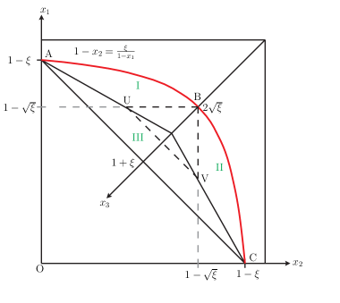
Figure 1: Dalitz plot showing phase space for $\gamma\rightarrow q\bar{q}g$ with off-shell gluon. The energy momentum conservation condition $x_{1}+x_{2}+x_{3}=2$ is satisfied throughout this $x_{1}-x_{2}$ plane and the actual length along $x_{3}$ axis is $\sqrt{2}$ times the measured length. The collinear limit (when the gluon is collinear to the quark) corresponds to $x_{1}=1-\xi$, $x_{2}=0$, while the soft limit (when the gluon is soft to the quark) corresponds to $x_{1}=x_{2}=1-\sqrt{\xi}$. The soft boundary of the phase space $1-x_{2}=\xi/(1-x_{1})$ is denoted by the red curve.

3.1 Thrust

Thrust is one of the most studied event shapes and it has a historical connection with the determination of strong coupling constant $\alpha_{s}$. It is defined as Farhi:1977sg

$$T=\underset{{\bf{n}}}{\text{Max}}\,\,\frac{\sum_{i}|{\bf p}_{i}\cdot{\bf{n}}|}{\sum_{i}E_{i}},$$ (14)

where ${\bf p}_{i}$ denotes the 3-momentum of the $i$-th particle in the final state and n is a unit vector. In order to determine the range of $T$, we need to consider two extreme cases: a most spherical configuration and a pencil like configuration. For a spherical configuration, $T$ attains a minimum value $1/2$ and for a pencil like configuration, $T$ attains a maximum value $1$. Thus, thrust varies in the range $1/2\leq T\leq 1$. For a three particles final state, the numerator in Eq. (14) is maximum when ${\bf{n}}$ is along the direction of the largest ${\bf{p_{i}}}$. Thus, the thrust for all massless particles final state is given by

$$T=\text{Max}\{x_{1},x_{2},x_{3}\}.$$ (15)

In presence of a massive off-shell gluon in the final state, the definition of thrust needs some simple modifications which was first given in Gardi:1999dq and has the form,

$$T=\text{Max}\left\{x_{1},x_{2},\sqrt{x_{3}^{2}-4\xi}\right\}.$$ (16)

Substituting in the definition Eq. (4) of the characteristic function, the squared matrix element Eq. (13) and the definition of thrust Eq. (16), we obtain

$$\mathcal{F}(T,\xi)=\int\int dx_{1}\ dx_{2}\frac{2}{(1-x_{1})(1-x_{2})}\delta\left(T-\text{Max}\left\{x_{1},x_{2},\sqrt{x_{3}^{2}-4\xi}\right\}\right).$$ (17)

When the radiated (dressed) gluon is soft, this integral receives contributions from the regions I and II as shown in Figure (1). Region I contributes when $x_{1}$ is the largest, and region II contributes when $x_{2}$ is the largest of $x_{1},x_{2},\sqrt{x_{3}^{2}-4\xi}$. Naming these contributions as $\mathcal{F}_{1}(T,\xi)$ and $\mathcal{F}_{2}(T,\xi)$ respectively, we have

$$\mathcal{F}(T,\xi)\simeq\mathcal{F}_{1}(T,\xi)+\mathcal{F}_{2}(T,\xi),$$ (18)

where

$$\mathcal{F}_{1}(T,\xi)= \int_{2-T-\sqrt{T^{2}+4\xi}}^{\frac{1-\xi-T}{1-T}}dx_{2}\ \mathcal{M}(T,x_{2},\xi)$$

$$\mathcal{F}_{2}(T,\xi)= \int_{2-T-\sqrt{T^{2}+4\xi}}^{\frac{1-\xi-T}{1-T}}dx_{1}\ \mathcal{M}(x_{1},T,\xi),$$ (19)

Note that the integrals $\mathcal{F}_{1}$ and $\mathcal{F}_{2}$ are same due to the symmetry of $\mathcal{M}(x_{1},x_{2},\xi)$ under interchange of $x_{1}$ and $x_{2}$. The limits of the integration are determined by the boundary of the phase space shown in red in the Figure (1). The characteristic function immediately evaluates to

$$\mathcal{F}\left(t,\xi\right)=-\frac{4}{t}\text{log}\bigg{(}\frac{\xi}{t(q-t)}\bigg{)},$$ (20)

where $t\equiv 1-T$ and $q=\sqrt{T^{2}+4\xi}$. Now, using Eqs. (6) and (20) the Borel function for the thrust takes the form,

$$B(t,u)= \frac{4\sin\pi u}{\pi u}\frac{1}{t}e^{\frac{5u}{3}}\int_{t^{2}}^{t}\xi^{-u-1}d\xi,$$ (21)

where the lower limit is determined using the collinear gluon boundary conditions, $x_{1}=1-\xi$, $x_{2}=0$ and the upper limit is determined from the soft gluon boundary condition $x_{1}=x_{2}=1-\sqrt{\xi}$. Evaluating the integral we immediately obtain

$$B(t,u)= \frac{\sin\pi u}{\pi u}e^{\frac{5u}{3}}\frac{4}{u}\frac{1}{t}\bigg{(}\frac{1}{t^{2u}}-\frac{1}{t^{u}}\bigg{)},$$ (22)

this agrees with the leading singular terms of the same function presented in Gardi:2001ny . Thus, it is possible to calculate the leading singular terms in $\mathcal{F}\left(t,\xi\right)$ and $B(t,u)$ using the eikonal matrix element.

3.2 $C$-parameter

The $C$-parameter was originally defined in Parisi:1978eg ; Donoghue:1979vi using the eigenvalues of the matrix

$$\theta_{\alpha\beta}=\frac{1}{\sum_{j}|\textbf{p}^{(j)}|}\sum_{i}\frac{\textbf{p}_{\alpha}^{(i)}\textbf{p}_{\beta}^{(i)}}{|\textbf{p}^{(i)}|},$$ (23)

where $\textbf{p}_{\alpha}^{(i)}$ are the spatial component of the momentum of $i$-th particle. If the eigenvalues of the above matrix are denoted by $\lambda_{1}$, $\lambda_{2}$ and $\lambda_{3}$, then the $C$-parameter is given by

$$C=3(\lambda_{1}\lambda_{2}+\lambda_{2}\lambda_{3}+\lambda_{1}\lambda_{3}).$$ (24)

This can be cast into a Lorentz invariant form

$$C=3-\frac{3}{2}\sum_{i,j}\frac{\left(p^{(i)}\cdot p^{(j)}\right)^{2}}{(p^{(i)}\cdot q)(p^{(j)}\cdot q)},$$ (25)

where $p^{(i)}$ denotes the four momentum of the $i$-th particle and $q$ denotes the total four-momentum. $C$ takes a minimum value $0$ for a two-jet event and $C$ attains a maximum value $1$ for a spherical event. If, however, the final state has a planar configuration the largest value that the parameter can attain is $3/4$. This upper limit also applies for the case of 3-body final state that concerns us. The above expression of the $C$-parameter and its rescaled version can be written down using the energy fractions and the virtuality of the off-shell gluon.

$$c=\frac{C}{6}=\frac{(1-x_{1})(1-x_{2})(x_{1}+x_{2}-1+2\xi)-\xi^{2}}{x_{1}x_{2}(2-x_{1}-x_{2})}.$$ (26)

Now, we define the eikonalized version of the $c$-parameter

$$c_{eik}(x_{1},x_{2})=\frac{(1-x_{1})(1-x_{2})}{(1-x_{1})+(1-x_{2})},$$ (27)

which coincides with the above definition in the soft gluon limit. Note that $c_{eik}$ is not a function of the virtuality $\xi$. We will use $c_{eik}$ to calculate the characteristic function for $C$-parameter; it is convenient to change variables from $x_{1}$ and $x_{2}$ into $y=2-x_{1}-x_{2}$ and $z=(1-x_{2})/y$. In these new variables $c_{e}ik(y,z)=yz(1-z)$. The characteristic function (Eq. (4)) in this limit takes the form,

$$\mathcal{F}=\int dy\ dz\ y\ \mathcal{M}_{\text{soft}}(y,z,\xi)\ \delta(c_{eik}(y,z)-c),$$ (28)

where,

$$\mathcal{M}_{\text{soft}}(y,z,\xi)=\frac{2}{y^{2}z(1-z)}$$ (29)

The symmetry of $\mathcal{M}$ under $x_{1}\leftrightarrow x_{2}$ appears as symmetry under $z\rightarrow 1-z$. In order to perform the integral in Eq. (28), it is required to determine the limits of the $z$-integration using the boundary of the soft region that is given by $x_{2}=(1-\xi-x_{1})/(1-x_{1})$. The integral in Eq. (28) has an explicit form,

$$\begin{split}\mathcal{F}=\int_{2\sqrt{\xi}}^{1+\xi}dy&\int_{\frac{1}{2}-\frac{1}{2}\sqrt{1-4\xi/y^{2}}}^{\frac{1}{2}+\frac{1}{2}\sqrt{1-4\xi/y^{2}}}dz\,\,\frac{2}{yz(1-z)}\frac{1}{y\sqrt{1-4c/y}}\,\,\Big{(}\delta(z-z_{1})+\delta(z-z_{2})\Big{)},\end{split}$$ (30)

where

$$z_{1}=\frac{1}{2}+\frac{1}{2}\sqrt{1-4c/y}\quad\text{and}\quad z_{2}=\frac{1}{2}-\frac{1}{2}\sqrt{1-4c/y}.$$ (31)

This integral has a symmetry under $z\leftrightarrow(1-z)$ interchange, therefore the integral over $z$ equals twice the integral between $z=1/2$ and the upper limit in Eq. (30), where only the $\delta(z-z_{1})$ is relevant. The condition $z\leq\frac{1}{2}+\frac{1}{2}\sqrt{1-4\xi/y^{2}}$ implies that $y\geq\xi/c$. With this the integral in Eq. (30) takes the form

$$\mathcal{F}=\frac{4}{c}\int_{\xi/c}^{1+\xi}dy\,\,\frac{1}{y\sqrt{1-4c/y}}.$$ (32)

Evidently, it is only the lower limit of the integration that gives rise to singular contribution in the $\xi\rightarrow 0$ limit. As we are only interested in the derivative of ${\cal F}$, we get, without even evaluating the integral

$$\frac{d\mathcal{F}}{d\xi}=-\frac{4}{c\xi}\frac{\sqrt{\xi}}{\sqrt{\xi-4c^{2}}}.$$ (33)

Contrast this to the computation of $d{\cal F}/{d\xi}$ presented in Gardi:2003iv where the computation proceeds with the full definition of the $c$-parameter. In that paper the authors had to deal with the complicated elliptic integrals and had to carefully consider small $c$ and small $\xi$ limits. These complications are completely absent in our method.

Now we are in the position to compute the Borel function $B(c,u)$ for the $c$-parameter. We have to substitute $d{\cal F}/{d\xi}$ into Eq. (5),

$$B(c,u)=\frac{4\sin{\pi u}}{\pi u}\frac{1}{c}e^{\frac{5u}{3}}\int_{4c^{2}}^{\frac{c}{1-c}}d\xi~{}\frac{\xi^{-u}}{\sqrt{\xi(\xi-4c^{2})}}$$ (34)

where the lower limit in the above integral is determined using $x_{1}=x_{2}=1-\sqrt{\xi}$ (soft limit), and the upper limit is determined using $x_{1}=1-\xi$, $x_{2}=0$ (collinear limit). We are interested in the logarithmically enhanced terms, thus we can replace the upper limit of the integration by $c/(1-c)\approx c$. Carrying out the integral yields the Borel function

$$B(c,u)=4\frac{\text{sin}\pi u}{\pi u}e^{\frac{5u}{3}}\frac{1}{c}\bigg{[}\frac{1}{(2c)^{2u}}\frac{\sqrt{\pi}\Gamma(u)}{\Gamma(u+\frac{1}{2})}-\frac{1}{uc^{u}}\bigg{]}.$$ (35)

Our result agrees with the soft contribution of the same function presented in Gardi:2003iv . We conclude thus, that the leading singular terms in $\mathcal{F}(c,\xi)$ and $B(c,\xi)$ can be captured with significant ease if we use the eikonal version $c_{eik}$ that we have introduced for the $c$-parameter.

3.3 Angularities

As a demonstration of the wide applicability of our method we consider one more event shape variable – the angularities. Angularities are novel observables that allow us to transform between recoil-insensitive to recoil-sensitive observables in a continuous manner. Angularities were first introduced almost twenty years ago in Berger:2003pk ; Berger:2003iw ; Berger:2002ig and they were defined as

$$\tau_{a}=\frac{1}{Q}\sum_{i}E_{i}(\sin\theta_{i})^{a}(1-|\cos\theta_{i}|)^{1-a},$$ (36)

where $\theta_{i}$ is the angle made by $i$-th particle with the thrust axis, $E_{i}$ is the energy of the particle $i$ and $a$ is a continuous parameter. The thrust axis is defined as the axis with respect to which Eq. (36) is minimized at $a=0$. One can easily realize that angularities with $a=0$ corresponds to $1-T$, where $T$ is the thrust, while $a=1$ refers to jet broadening Catani:1992jc . The continuous parameter $a$ has a range $-\infty<a<2$, where the upper limit on $a$ is fixed by infrared safety. In terms of $x_{i}$ and $\xi$ angularities were defined in Berger:2004xf as,

$$\tau_{a}(x_{1},x_{2},\xi)= \frac{1}{x_{1}}(1-x_{1})^{1-a/2}\bigg{[}(1-x_{2}-\xi)^{1-a/2}(x_{1}+x_{2}-1+\xi)^{a/2}$$

$$+(1-x_{2}-\xi)^{a/2}(x_{1}+x_{2}-1+\xi)^{1-a/2}\bigg{]},$$ (37)

where, thrust axis is considered along $\textbf{p}_{1}$ (quark momentum). As we did for the $c$-parameter we introduce an eikonal version of the angularities:

$$\tau_{a}^{eik}(x_{1},x_{2},\xi)=(1-x_{1})^{1-a/2}(1-x_{2})^{a/2}.$$ (38)

Now, Using Eq. (4) and (13) the characteristics function takes the form,

$$\mathcal{F}=\int dx_{1}dx_{2}\frac{2}{(1-x_{1})(1-x_{2})}\delta\big{(}\tau_{a}^{eik}(x_{1},x_{2},\xi)-\tau_{a}\big{)}.$$ (39)

It is straight-forward to perform the $x_{1}$ integration to obtain

$$\mathcal{F} =\frac{4}{\tau_{a}(1-\frac{a}{2})}\int dx_{2}\,\frac{1}{1-x_{2}}.$$ (40)

We determine the upper limit of this integration using the soft boundary $1-x_{2}=\xi/(1-x_{1})$. As shown in Berger:2004xf , the lower limit of this integration does not contribute to the logarithmically enhanced terms. The upper limit of the integration is

$$1-\bigg{(}\frac{\xi^{1-\frac{a}{2}}}{\tau_{a}}\bigg{)}^{\frac{1}{1-a}}.$$

We finally have the characteristics function

$$\mathcal{F}(\tau_{a},\xi)=-\frac{4}{\tau_{a}}\frac{1}{1-a}\log\xi.$$ (41)

Taking the derivative with respect to $\xi$ and substituting in Eq. (6) we get the Borel function

$$B(\tau_{a},u)=\frac{4\sin{\pi u}}{\pi u}\frac{1}{1-a}\frac{1}{\tau_{a}}e^{\frac{5u}{3}}\int_{\tau_{a}^{2}}^{\tau_{a}^{\frac{2}{2-a}}}d\xi~{}\xi^{-u-1},$$ (42)

where the limits are determined using the collinear and soft gluon boundary conditions mentioned in Figure (1). Upon performing the integration in Eq. (42) we obtain

$$B(\tau_{a},u)=\frac{\sin{\pi u}}{\pi u}e^{\frac{5}{3}u}\frac{4}{1-a}\frac{1}{u}\frac{1}{\tau_{a}}\left[\frac{1}{\tau_{a}^{2u}}-\frac{1}{\tau_{a}^{\frac{2u}{2-a}}}\right]\,,$$ (43)

which agrees with the soft contribution of the same function presented in Berger:2004xf . We have, thus obtained, the leading singular terms in $\mathcal{F}(\tau_{a},\xi)$ and $B(\tau_{a},\xi)$, which are responsible for power corrections by considering the eikonal matrix element and the eikonal version of the angularities $\tau_{a}^{eik}(x_{1},x_{2},\xi)$ which again substantially simplifies the computation.

4 Borel function using Eikonal Dressed Gluon Exponentiation
in the light-cone variables

In this section, we will follow the same steps of Sec. (3) and calculate Borel function for thrust, $C$-parameter and angularities using a different set of kinematic variables. Instead of the energy fractions that we used in the previous section we would employ the transverse momentum $k_{\perp}$ and rapidity $y$ of the massive eikonal gluon. In the soft gluon approximation, a number of event shapes for massless particles were defined in  Salam:2001bd ; Mateu:2012nk . We will consider a class of event shapes which, for massive soft gluon emission, can be written as

$$\bar{e}(k,Q)\,=\,\sqrt{\frac{k_{\perp}^{2}+k^{2}}{Q^{2}}}~{}h_{e}(y)\,,$$ (44)

where $k_{\perp}$ and $y$ denote transverse momentum of the gluon and pseudo-rapidity measured with respect to the thrust axis respectively. The function $h_{e}(y)$ characterizes the given event shape. Some of the approximations described below apply to more general event shapes as well, but the results are especially simple for those which can be cast in the form of Eq. (44).

The contribution from the emission of a soft off-shell gluon can easily be computed applying the eikonal approximation to the vertex for the emission from the hard parton. Since off-shell soft-gluon phase space factorizes Gardi:2001di from the hard partons, and also the matrix element factorizes, the soft cross section takes on a simple and universal form,

$$\frac{d\sigma}{\sigma}\,=\,\frac{1}{3}\,\frac{4}{k^{2}+k_{\perp}^{2}}\,dk_{\perp}^{2}dy\,.$$ (45)

The characteristic function is also then given, in the soft limit, by a simple and universal expression

$$\mathcal{F}(e,\xi)=\int dk_{\perp}^{2}dy\,\frac{2}{k^{2}+k_{\perp}^{2}}\delta\left(e-\bar{e}\left(k^{2},k_{\perp}^{2},y\right)\right)\,,$$ (46)

which integrates to the remarkably simple form,

$$\mathcal{F}(e,\xi)\,=\,\frac{8}{e}\int_{y_{{\rm min}}}dy\,$$ (47)

where the only information on the chosen observable is the phase space boundary given by the minimum rapidity $y_{{\rm min}}$. The upper limit of integration is not relevant, since it does not give any singular contributions in the $\xi\rightarrow 0$ limit, which is the only significant limit for power corrections.

Up to now, we have kept the discussion generic, for any shape belonging to the class given in Eq. (44). Let us now illustrate the results by looking at some specific examples.

4.1 Thrust

The thrust for a generic process is defined in Eq. (15). In the two jet events all event shape variables that we consider tends to $0$, except thrust which tends to 1. Thus, it is convenient to define $t=1-T$. In the soft gluon approximation, thrust in terms of the $k_{\perp}$ and rapidity $y$ is given by Salam:2001bd

$$t=\frac{1}{Q}\sqrt{k_{\perp}^{2}+k^{2}}\ e^{-|y|}.$$ (48)

Note that, for our case the gluon is massive and $k^{2}\neq 0$. In order to perform the integral in Eq. (47), we need to determine the lower limit of the rapidity. The lower limit of rapidity $y$ is determined by putting $k_{\perp}=0$ in Eq. (48), thus minimum rapidity is given by,

$$y_{{\rm min}}\,=\,\,\ln\Big{(}\frac{1}{t}\sqrt{\xi}\Big{)}.$$ (49)

Now, using Eq. (47) and (49) the characteristics function has the form,

$$\mathcal{F}=-\frac{8}{t}\text{log}(\frac{\sqrt{\xi}}{t}).$$ (50)

The Borel function $B(t,u)$ is then given by

$$B(t,u)=\frac{\sin{\pi u}}{\pi u}e^{\frac{5}{3}u}\frac{4}{u}\frac{1}{t}\left[\frac{1}{t^{2u}}-\frac{1}{t^{u}}\right]\,,$$ (51)

which is in well agreement with the soft approximated version of the characteristics function and Borel function presented in Gardi:2001ny .

4.2 $C$-parameter

The $C$-parameter for a generic process is defined in Eq. (3.2). The $C$-parameter in the soft approximation and expressed using $k_{\perp}$ and $y$ is given by Salam:2001bd

$$c=\frac{C}{6}=\frac{1}{2Q}\sqrt{k^{2}+k_{\perp}^{2}}\ \frac{1}{\text{cosh}\ y}.$$ (52)

As for the case of thrust we determine the lower limit of rapidity by putting $k_{\perp}=0$ and obtain

$$y_{{\rm min}}=\cosh^{-1}\left({\sqrt{\xi}}/(2c).\right).$$ (53)

Now, substituting $y_{\text{min}}$ in Eq. (47) we obtain the characteristic function in the soft gluon limit:

$$\mathcal{F}=-\frac{8}{c}\text{cosh}^{-1}\bigg{(}\frac{\sqrt{\xi}}{2c}\bigg{)}.$$ (54)

This yields the Borel function

$$B(c,u)=4\frac{\text{sin}\pi u}{\pi u}e^{5u/3}\frac{1}{c}\bigg{[}\frac{1}{(2c)^{2u}}\frac{\sqrt{\pi}\Gamma(u)}{\Gamma(u+\frac{1}{2})}-\frac{1}{uc^{u}}\bigg{]},$$ (55)

in full agreement with the soft contribution to the same function in Gardi:2003iv . Notice that, while collinear effects present in Gardi:2003iv are not properly reproduced, as expected, the cancellation of the pole at $u=0$, which is a consequence of the IR safety of the event shape, is preserved.

4.3 Angularities

In the soft gluon limit, angularities takes the form Salam:2001bd ; Mateu:2012nk ,

$$\tau_{a}=\frac{1}{Q}\sqrt{k^{2}+k_{\perp}^{2}}\ e^{-|y|(1-a)},$$ (56)

and the minimum rapidity is given by

$$y_{{\rm min}}\,=\,\frac{1}{1-a}\,\ln\Big{(}\frac{1}{\tau_{a}}\sqrt{\xi}\Big{)}\,.$$ (57)

Now, using Eq. (47), one easily finds

$$\frac{d\mathcal{F}(\tau_{a},\xi)}{d\xi}\,=\,-\frac{1}{1-a}\,\frac{4}{\tau_{a}\xi}\,.$$ (58)

The Borel function $B(\tau_{a},u)$ is then given by

$$B(\tau_{a},u)=\frac{\sin{\pi u}}{\pi u}e^{\frac{5}{3}u}\frac{4}{1-a}\frac{1}{u}\frac{1}{\tau_{a}}\left[\frac{1}{\tau_{a}^{2u}}-\frac{1}{\tau_{a}^{\frac{2u}{2-a}}}\right]\,,$$ (59)

again in agreement with the soft contribution to the results of Berger:2004xf , and reproducing, in the limit $a\to 0$, the results for thrust of Ref. Gardi:2002bg .

5 The Sudakov exponent

In this section, we will describe the computation of Sudakov exponent for thrust. Similar conclusions hold true for the other two shape variables as well that we have considered in this article. We can calculate the Borel function in the Laplace space $B_{\nu}^{t}(u)$ in the eikonal limit using $B(t,u)$ that we wrote above in Eq. (22), we obtain,

$$B_{\nu}^{t,\text{eik}\text{ }}(u) =\frac{4\,\text{sin}\,\pi u}{\pi u}\,e^{\frac{5u}{3}}\,\frac{1}{u}\,\bigg{[}\bigg{(}\nu^{2u}\gamma(-2u,\nu)+\frac{1}{2u}\bigg{)}-\bigg{(}\nu^{u}\gamma(-u,\nu)+\frac{1}{u}\bigg{)}\bigg{]},$$ (60)

where, we have used

$$\int_{0}^{1}\frac{dt}{t}\,e^{u\,\text{log}\frac{1}{t}}\,(e^{-\nu t}-1)=\nu^{u}\gamma(-u,\nu)+\frac{1}{u},$$ (61)

and $\gamma(-u,\nu)=\Gamma(-u)-\Gamma(-u,\nu)$. In the Sudakov region ($\nu\rightarrow\infty$), we can replace $\gamma(-u,\nu)$ by $\Gamma(-u,\nu)$. Retaining only the logarithmically enhanced terms (powers of log  $\nu$), in the small $u$ limit $B_{\nu}^{t}(u)$ takes the form,

$$B_{\nu}^{t,\text{{eik}}}(u)=2\,e^{\frac{5}{3}u}\frac{\,\text{sin\,}\pi u}{\pi u}\bigg{[}\Gamma(-2u)\>\bigg{(}\nu^{2u}-1\bigg{)}\frac{2}{u}-\Gamma(-u)\>\bigg{(}\nu^{u}-1\bigg{)}\frac{2}{u}\bigg{]}$$ . (62)

The first term inside the square brackets corresponds to large-angle soft gluon emissions and the second term to collinear gluon emissions. Note that this expression is free from any $u=0$ singularities. There are two sources of the poles in this expression: $\Gamma(-2u)$ has poles for all positive integers and half-integers, and $\Gamma(-u)$ has poles for all positive integers. However, the pre-factor sin $\pi u$ regulates the poles at the integer values of $u$. Thus, $B_{t}^{\nu,\text{eik}}$ has renormalon poles only at half-integer values of $u$.

We will now compare our result with the full result for $B_{\nu}^{t}$ presented in Gardi:2001ny ; Gardi:2003iv which is given by,

$$B_{\nu}^{t}(u)=\,2{\rm e}^{\frac{5}{3}u}\,\frac{\sin\pi u}{\pi u}\left[\Gamma(-2u)\left(\nu^{2u}-1\right)\frac{2}{u}-\Gamma(-u)\left(\nu^{u}-1\right)\left(\frac{2}{u}+\frac{1}{1-u}+\frac{1}{2-u}\right)\right]\,.$$ (63)

Note the poles at $u=1$ and $u=2$ which are absent in the collinear term of our eikonalized $B_{\nu}^{t,\text{eik}}(u)$. We further notice that no spurious renormalon poles are present in the eikonalized version. Recall that, for thrust approximation was done only for the matrix element and not for the definition of the variable. To show that our eikonal versions of the shape variables do not spoil the above feature we present the results for the $c$-parameter. The eikonal version and full result Gardi:2003iv are as follows:

$$B_{\nu}^{c,\text{eik}}(u) =2\,\frac{\sin\,\pi u}{\pi u}e^{\frac{5u}{3}}\,\bigg{[}\Gamma(-2u)(\nu^{2u}-1)2^{1-2u}\frac{\sqrt{\pi}\Gamma(u)}{\Gamma(u+\frac{1}{2})}-\frac{2}{u}\Gamma(-u)(\nu^{u}-1)\bigg{]},$$ (64)

$$B_{\nu}^{c}(u) =2\,\frac{\sin\,\pi u}{\pi u}e^{\frac{5u}{3}}\,\left[\Gamma(-2u)\left(\nu^{2u}-1\right)2^{1-2u}\frac{\sqrt{\pi}\Gamma(u)}{\Gamma(\frac{1}{2}+u)}\right.$$

$$\hskip 115.0pt-\left.\Gamma(-u)\left({\nu}^{u}-1\right)\left(\frac{2}{u}+\frac{1}{1-u}+\frac{1}{2-u}\right)\right]\,.$$ (65)

Again, no spurious poles are introduced. As expected, the EDGE does not reproduce the collinear renormalon singularities as it cannot capture the hard-collinear emissions correctly.

The perturbative coefficients of the Sudakov exponent in the large-$\beta_{0}$ limit can be determined by expanding $B_{\nu}^{t}(u)$ in powers of $u$ and replacing $u^{n}$ by $n!/(\beta_{0}\alpha_{s}/\pi)^{n+1}$. We notice that the large-angle soft gluon emission terms – the coefficient of $\Gamma(-2u)$, are identical in the eikonalized and full versions of the Borel function in the Laplace space. This implies that the leading logs – the terms of the form $L^{n+1}\alpha_{s}^{n}$ where $L=\text{log $\nu$ }$, will be the same between the two. The differences in the sub-leading logarithms appear due to the absence of the $u=1$ and $u=2$ poles in the collinear terms. We will now expand the two functions to the first few orders to demonstrate the matching of the LL terms and the discrepancy in the sub-leading logarithms. The expansion of the full result gives,

$$B_{\nu}^{t}\left(u\right) =-2\,L^{2}+0.691\,L$$

$$+\,\left(-2\,L^{3}-5.297\,L^{2}-6.485\,L\right)\,u$$

$$+\,\left(-1.167\,L^{4}-5.527\,L^{3}-14.491\,L^{2}-31.655\,L\right)\,u^{2}$$

$$+\,\left(-0.5\,L^{5}-3.262\,L^{4}-12.329\,L^{3}-39.003\,L^{2}-80.940\,L\right)\,u^{3}$$

$$+\,\left(-0.172\,L^{6}-1.405\,L^{5}-6.832\,L^{4}-28.452\,L^{3}-87.21\,L^{2}-175.80\,L\right)\,u^{4}$$ (66)

$$+\mathcal{O}(u^{5})+\ldots$$

whereas, the expansion of the eikonal result gives,

$$B_{\nu}^{t,\text{eik}}(u)= -2\>L^{2}-2.31\>L$$

$$+\> (-2\,L^{3}-6.79\,L^{2}-15.71\,L)\>u$$

$$+\, (-1.167\,L^{4}-6.02\,L^{3}-19.10\,L^{2}-44.59\,L)\>u^{2}$$

$$+\, (-0.5\,L^{5}-3.38\,L^{4}-13.86\,L^{3}-45.47\,L^{2}-93.66\,L)\>u^{3}$$

$$+\, (-0.172\,L^{6}-1.429\,L^{5}-7.216\,L^{4}-30.61\,L^{3}-93.57\,L^{2}-187.395\,L)\>u^{4}$$ (67)

$$+\, \mathcal{{O}}(u^{5})+\ldots\>\,.$$

As expected, the leading logarithms are appearing correctly in the eikonal approximated version of the Borel function in the Laplace space. We observe that the differences in NLL and NNLL terms between $B_{\nu}^{t}$ and $B_{\nu}^{t,\text{eik}}$ are decreasing as we go higher order in $u$.

Let us now discuss the power corrections. The Sudakov exponent is an integral over $u$ and the poles of $B_{\nu}^{t}$ that occur on the real $u$-axis make it an ill defined integral. The integral can be defined by shifting the poles above or below the axis or equivalently indenting the contour below or above the poles. This however, introduces an ambiguity that is proportional to the residue of the poles. The poles of $B_{\nu}^{t}$ that occur at $u=m/2$, where $m$ is an odd integer give the ambiguity Gardi:2003iv originating from the large-angle soft gluon emissions. From Eq. (9) we see that the ambiguity would be of the form $(\Lambda\nu/Q)^{m}$ which implies the existence of non-perturbative power corrections of the same form. In Table (1) we present the residues of poles at $u=m/2$ arising from $B_{\nu}^{t,\text{eik}}(u)$ which contribute to the soft power corrections. The full result $B_{\nu}^{t}(u)$ also has poles at $u=1$ and $u=2$ which give indications to the size of the collinear power corrections whereas these are absent in $B_{\nu}^{t,\text{eik}}(u)$. Thus, the collinear power corrections exist only for $\nu^{1}$ and $\nu^{2}$, and using the full expression for $B_{\nu}^{t}(u)$ we find that they are given by $-2\big{(}\frac{\overline{\Lambda}}{Q}\big{)}^{2}$ and $-\frac{1}{2}\big{(}\frac{\overline{\Lambda}}{Q}\big{)}^{4}$ respectively. Note that, in the calculation of the residues for the collinear terms we have ignored the $\mathcal{O}(1)$ factor $C_{F}/2\beta_{0}$. We see, thus, that the residue of the collinear power correction is suppressed by $\bar{\Lambda}/Q$ as compared to the soft correction for $\nu^{1}$ term. For example at the LEP where $Q=209$ Gev and $\bar{\Lambda}=200\>e^{\frac{5}{6}}$ Mev, the ratio of the size of the collinear correction to the soft correction for $\nu^{1}$ is approximately $-0.0017$. Thus, at colliders like LEP, the soft power corrections are more important as compared to the collinear corrections. As pointed out in Gardi:2001ny , the dominant power correction arising from the residue at $u=1/2$ is proportional to $\nu$ and thus generates a shift in the resummed cross-section.

For the other event shapes considered in this article one can calculate the Borel function in Laplace space using EDGE. It remains true that soft power corrections are dominant over the collinear corrections for all the event shapes considered in this paper.

Correction	Residue
$\nu^{1}$	8$\frac{\overline{\Lambda}}{Q}$
$\nu^{3}$	$-\frac{4}{27}\big{(}\frac{\overline{\Lambda}}{Q}\big{)}^{3}$
$\nu^{5}$	$\frac{1}{375}\big{(}\frac{\overline{\Lambda}}{Q}\big{)}^{5}$
$\nu^{7}$	$-\frac{1}{30870}\big{(}\frac{\overline{\Lambda}}{Q}\big{)}^{7}$

Table 1: The size of the residues of renormalon singularities for soft power corrections. The numbers quoted are $\pi$ times the residue and $\overline{\Lambda}=\Lambda\>e^{5/6}$. We ignore here the $\mathcal{O}(1)$ factor $C_{F}/2\beta_{0}$ in Eq. (9).

6 Conclusions

In this paper, we have introduced Eikonal Dressed Gluon Exponentiation which is a combination of Dressed Gluon Exponentiation and Eikonal approximation. Using our method, we have demonstrated for several event shapes at $e^{+}e^{-}$ colliders that the leading singular contributions for the respective Borel functions in the single dressed gluon approximation are produced with remarkably simple calculations. It is straightforward to construct the Sudakov exponent in the large-$\beta_{0}$ limit for the power corrections using the procedure presented in  Gardi:2001di ; Gardi:1999dq . This exponentiation effectively resums both the large Sudakov logarithms and the power corrections. We observe that EDGE does not introduce any spurious renormalons and correctly produces the dominant power corrections originating from soft emissions.

We have shown that in order to accurately capture the leading singular terms of the characteristic function $\mathcal{F}(e,\xi)$ and Borel function $B(e,\xi)$ for an event shape variable $e$, it is sufficient to use the eikonal squared matrix element $\mathcal{M}$, together with the eikonal version of the event shape variable. Typically the shape variables such as $C$-parameter and angularities have complicated expressions especially so when the final state gluon is off the mass shell. We have demonstrated that the simplification of the computations is achieved, both when one uses the energy fractions as the variables, and also when we uses light-cone variables to parameterize the phase space of the eikonal dressed gluon. When using the latter variables, we observe that the minimum value of rapidity $y_{\text{min}}$ is the source of the leading singular terms in $\mathcal{F}(e,\xi)$. We believe that this method is sufficiently simple and flexible to be implemented also in the more intricate environment of hadron collisions, where hadronic event shapes and jet shapes provide important tools for QCD analyses.

7 Acknowledgments

SP and AM would like to thank MHRD Govt. of India for an SRF fellowship. AT would like to thank Lorenzo Magnea for suggesting this project and for very fruitful discussions, Einan Gardi for very useful discussions, and the University of Turin and INFN Turin for warm hospitality during the course of this work.

References

- (1) A. Gehrmann-De Ridder, T. Gehrmann, E. Glover and G. Heinrich, NNLO corrections to event shapes in annihilation, JHEP 0712 (2007) 094 [0711.4711].
- (2) S. Weinzierl, Event shapes and jet rates in electron-positron annihilation at NNLO, JHEP 0906 (2009) 041 [0904.1077].
- (3) T. Gehrmann, A. Huss, J. Mo and J. Niehues, Second-order QCD corrections to event shape distributions in deep inelastic scattering, Eur. Phys. J. C 79 (2019) 1022 [1909.02760].
- (4) A. Kardos, G. Somogyi and A. Verbytskyi, Determination of beyond NNLO using event shape moments, 2009.00281.
- (5) A. Gehrmann-De Ridder, T. Gehrmann, E. Glover and G. Heinrich, NNLO moments of event shapes in e+e- annihilation, JHEP 05 (2009) 106 [0903.4658].
- (6) S. Catani, L. Trentadue, G. Turnock and B. Webber, Resummation of large logarithms in e+ e- event shape distributions, Nucl.Phys. B407 (1993) 3.
- (7) A. Banfi, G. P. Salam and G. Zanderighi, Phenomenology of event shapes at hadron colliders, JHEP 06 (2010) 038 [1001.4082].
- (8) A. Banfi, G. P. Salam and G. Zanderighi, Principles of general final-state resummation and automated implementation, JHEP 03 (2005) 073 [hep-ph/0407286].
- (9) A. Banfi, G. Salam and G. Zanderighi, Semi-numerical resummation of event shapes, JHEP 0201 (2002) 018 [hep-ph/0112156].
- (10) A. Banfi, H. McAslan, P. F. Monni and G. Zanderighi, The two-jet rate in at next-to-next-to-leading-logarithmic order, Phys. Rev. Lett. 117 (2016) 172001 [1607.03111].
- (11) R. Abbate, M. Fickinger, A. H. Hoang, V. Mateu and I. W. Stewart, Thrust at LL with Power Corrections and a Precision Global Fit for alphas(mZ), Phys.Rev. D83 (2011) 074021 [1006.3080].
- (12) T. Becher and G. Bell, NNLL Resummation for Jet Broadening, JHEP 1211 (2012) 126 [1210.0580].
- (13) A. H. Hoang, D. W. Kolodrubetz, V. Mateu and I. W. Stewart, -parameter distribution at N3LL’ including power corrections, Phys. Rev. D 91 (2015) 094017 [1411.6633].
- (14) A. Budhraja, A. Jain and M. Procura, One-loop angularity distributions with recoil using Soft-Collinear Effective Theory, JHEP 08 (2019) 144 [1903.11087].
- (15) G. Bell, A. Hornig, C. Lee and J. Talbert, angularity distributions at NNLL′ accuracy, JHEP 01 (2019) 147 [1808.07867].
- (16) A. H. Hoang, D. W. Kolodrubetz, V. Mateu and I. W. Stewart, State-of-the-art predictions for C-parameter and a determination of , Nucl. Part. Phys. Proc. 273-275 (2016) 2015 [1501.04753].
- (17) D. W. Kolodrubetz, Accuracy and Precision in Collider Event Shapes, Ph.D. thesis, MIT, Cambridge, CTP, 2016. 1605.06435.
- (18) C. Lepenik and V. Mateu, NLO Massive Event-Shape Differential and Cumulative Distributions, JHEP 03 (2020) 024 [1912.08211].
- (19) C. Lee, A. Hornig and G. Ovanesyan, Probing the Structure of Jets: Factorized and Resummed Angularity Distributions in SCET, PoS EFT09 (2009) 010 [0905.0168].
- (20) A. Hornig, C. Lee and G. Ovanesyan, Effective Predictions of Event Shapes: Factorized, Resummed, and Gapped Angularity Distributions, JHEP 05 (2009) 122 [0901.3780].
- (21) A. Banfi, H. McAslan, P. F. Monni and G. Zanderighi, A general method for resummation of event-shape distributions in annihilation, JHEP 05 (2015) 102 [1412.2126].
- (22) I. I. Bigi, M. A. Shifman, N. Uraltsev and A. Vainshtein, The Pole mass of the heavy quark. Perturbation theory and beyond, Phys.Rev. D50 (1994) 2234 [hep-ph/9402360].
- (23) M. Beneke and V. M. Braun, Heavy quark effective theory beyond perturbation theory: Renormalons, the pole mass and the residual mass term, Nucl.Phys. B426 (1994) 301 [hep-ph/9402364].
- (24) B. Webber, Estimation of power corrections to hadronic event shapes, Phys.Lett. B339 (1994) 148 [hep-ph/9408222].
- (25) Y. L. Dokshitzer, G. Marchesini and B. Webber, Dispersive approach to power behaved contributions in QCD hard processes, Nucl.Phys. B469 (1996) 93 [hep-ph/9512336].
- (26) M. Dasgupta and G. P. Salam, Event shapes in e+ e- annihilation and deep inelastic scattering, J.Phys. G30 (2004) R143 [hep-ph/0312283].
- (27) A. H. Hoang, D. W. Kolodrubetz, V. Mateu and I. W. Stewart, Precise determination of from the -parameter distribution, Phys. Rev. D 91 (2015) 094018 [1501.04111].
- (28) S.-Q. Wang, S. J. Brodsky, X.-G. Wu, J.-M. Shen and L. Di Giustino, Novel method for the precise determination of the QCD running coupling from event shape distributions in electron-positron annihilation, Phys. Rev. D 100 (2019) 094010 [1908.00060].
- (29) S. Marzani, D. Reichelt, S. Schumann, G. Soyez and V. Theeuwes, Fitting the Strong Coupling Constant with Soft-Drop Thrust, JHEP 11 (2019) 179 [1906.10504].
- (30) T. Gehrmann, G. Luisoni and P. F. Monni, Power corrections in the dispersive model for a determination of the strong coupling constant from the thrust distribution, Eur. Phys. J. C 73 (2013) 2265 [1210.6945].
- (31) E. Gardi, Dressed gluon exponentiation, Nucl.Phys. B622 (2002) 365 [hep-ph/0108222].
- (32) E. Gardi and J. Rathsman, The Thrust and heavy jet mass distributions in the two jet region, Nucl.Phys. B638 (2002) 243 [hep-ph/0201019].
- (33) E. Gardi and L. Magnea, The C parameter distribution in e+ e- annihilation, JHEP 0308 (2003) 030 [hep-ph/0306094].
- (34) C. F. Berger and L. Magnea, Scaling of power corrections for angularities from dressed gluon exponentiation, Phys.Rev. D70 (2004) 094010 [hep-ph/0407024].
- (35) M. Cacciari and E. Gardi, Heavy quark fragmentation, Nucl.Phys. B664 (2003) 299 [hep-ph/0301047].
- (36) E. Gardi, Radiative and semileptonic B meson decay spectra: Sudakov resummation beyond logarithmic accuracy and the pole mass, JHEP 0404 (2004) 049 [hep-ph/0403249].
- (37) J. R. Andersen and E. Gardi, Taming the anti-B spectrum by dressed gluon exponentiation, JHEP 0506 (2005) 030 [hep-ph/0502159].
- (38) C. Lee, Universal nonperturbative effects in event shapes from soft-collinear effective theory, Mod. Phys. Lett. A 22 (2007) 835 [hep-ph/0703030].
- (39) E. Gardi, Perturbative and nonperturbative aspects of moments of the thrust distribution in e+ e- annihilation, JHEP 04 (2000) 030 [hep-ph/0003179].
- (40) E. Gardi and J. Rathsman, Renormalon resummation and exponentiation of soft and collinear gluon radiation in the thrust distribution, Nucl.Phys. B609 (2001) 123 [hep-ph/0103217].
- (41) S. Brandt, C. Peyrou, R. Sosnowski and A. Wroblewski, The Principal axis of jets. An Attempt to analyze high-energy collisions as two-body processes, Phys. Lett. 12 (1964) 57.
- (42) G. L. Kane, J. Pumplin and W. Repko, Transverse Quark Polarization in Large p(T) Reactions, e+ e- Jets, and Leptoproduction: A Test of QCD, Phys. Rev. Lett. 41 (1978) 1689.
- (43) E. Farhi, A QCD Test for Jets, Phys. Rev. Lett. 39 (1977) 1587.
- (44) G. Altarelli, Partons in Quantum Chromodynamics, Phys. Rept. 81 (1982) 1.
- (45) J. F. Donoghue, F. Low and S.-Y. Pi, Tensor Analysis of Hadronic Jets in Quantum Chromodynamics, Phys. Rev. D 20 (1979) 2759.
- (46) G. C. Fox and S. Wolfram, Observables for the Analysis of Event Shapes in e+ e- Annihilation and Other Processes, Phys. Rev. Lett. 41 (1978) 1581.
- (47) J. Bjorken and S. J. Brodsky, Statistical Model for electron-Positron Annihilation Into Hadrons, Phys. Rev. D 1 (1970) 1416.
- (48) G. Parisi, Super Inclusive Cross-Sections, Phys. Lett. B 74 (1978) 65.
- (49) C. F. Berger and G. F. Sterman, Scaling rule for nonperturbative radiation in a class of event shapes, JHEP 0309 (2003) 058 [hep-ph/0307394].
- (50) C. F. Berger, T. Kucs and G. F. Sterman, Event shape / energy flow correlations, Phys.Rev. D68 (2003) 014012 [hep-ph/0303051].
- (51) C. F. Berger, T. Kucs and G. F. Sterman, Interjet energy flow / event shape correlations, Int. J. Mod. Phys. A 18 (2003) 4159 [hep-ph/0212343].
- (52) E. Gardi and G. Grunberg, Power corrections in the single dressed gluon approximation: The Average thrust as a case study, JHEP 11 (1999) 016 [hep-ph/9908458].
- (53) S. Catani, G. Turnock and B. Webber, Jet broadening measures in annihilation, Phys. Lett. B 295 (1992) 269.
- (54) G. Salam and D. Wicke, Hadron masses and power corrections to event shapes, JHEP 05 (2001) 061 [hep-ph/0102343].
- (55) V. Mateu, I. W. Stewart and J. Thaler, Power Corrections to Event Shapes with Mass-Dependent Operators, Phys. Rev. D 87 (2013) 014025 [1209.3781].