Knowledge Capture and Replay for Continual Learning

Abstract

Deep neural networks have shown promise in several domains, and the learned data (task) specific information is implicitly stored in the network parameters. Extraction and utilization of encoded knowledge representations is vital when data is no longer available in the future, especially in a continual learning scenario. In this work, we introduce flashcards, which are visual representations that capture the encoded knowledge of a network as a recursive function of predefined random image patterns. In a continual learning scenario, flashcards help to prevent catastrophic forgetting and consolidating knowledge of all the previous tasks. Flashcards need to be constructed only before learning the subsequent task, and hence, independent of the number of tasks trained before. We demonstrate the efficacy of flashcards in capturing learnt knowledge representation (as an alternative to original dataset), and empirically validate on a variety of continual learning tasks: reconstruction, denoising, task-incremental learning, and new-instance learning classification, using several heterogeneous benchmark datasets. Experimental evidence indicates that: (i) flashcards as a replay strategy is task agnostic, (ii) performs better than generative replay, and (iii) is on par with episodic replay without additional memory overhead.

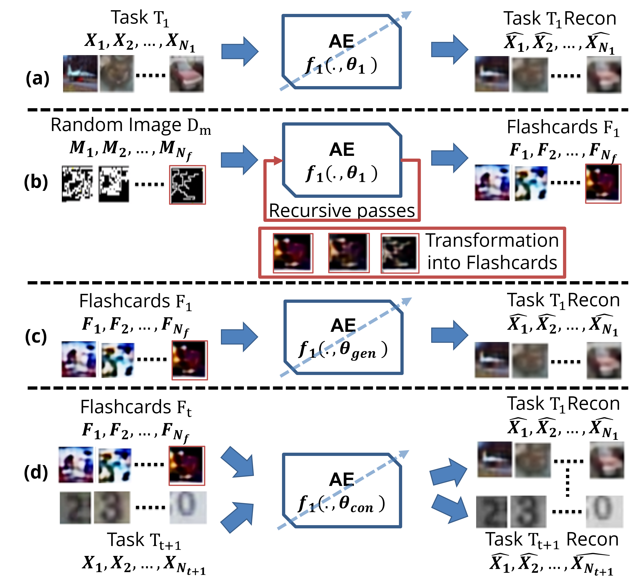
Figure 1: Flashcards for knowledge capture and replay. Step (a): Trained autoencoder (AE) for Task $T_{1}$; Step (b): Construct flashcards from frozen AE using maze patterns via recursive passes; Step (c): Replay using flashcards on a new network to remember Task $T_{1}$; Step (d) Replay using flashcards $F_{t}$ while training for Task $T_{t+1}$.

1 Introduction

Deep neural networks are successful in several applications (Krizhevsky et al., 2012; Devlin et al., 2019; Längkvist et al., 2014), however, it remains a challenge to extract and reuse the knowledge embedded in the representations of the trained models, in a benign manner, for similar or other downstream scenarios (Bing, 2020). Approaches such as transfer learning (Zhuang et al., 2021) and knowledge distillation (Gou et al., 2020) enable representational or functional translation (Hinton et al., 2015) from one model to the other. Importantly, knowledge captured from the past should be preserved in some representation with low computational and memory expense, especially, when the past data is no longer available.

Learning new tasks affects retention of previous knowledge (Robins, 1995). Continual learning (CL) (Thrun, 1996) was proposed as a candidate for such retention, and is gaining attention recently (Parisi et al., 2019). Essentially, CL aims to make deep neural networks learn continually from a sequence of tasks efficiently, without catastrophically forgetting the past sequences/tasks. There is a need to develop a reliable method that can effectively capture and re-purpose knowledge from a learned model, which can then be exploited in the CL setting. Also, while CL approaches are predominantly studied on classification (class/task incremental learning), its potential remains relatively less explored in other scenarios such as task agnostic unsupervised reconstruction, denoising, new instance learning, etc.

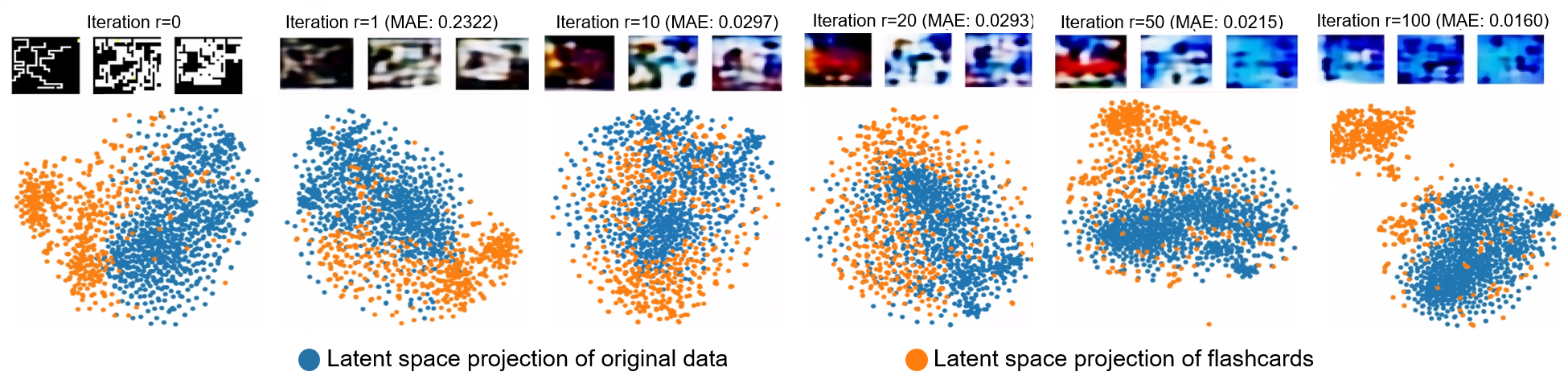
Figure 2: A sample of three Flashcards ($F_{t}$) constructions over recursive iterations, with Cifar10 as an example, difference in MAE between successive iterations with iteration number and t-SNE of latent space in 2D. It can be observed that the initial (raw) input maze patterns adapt to the texture captured by the model, as the number of recursive iterations increase (Iteration $r=10,20$). Also, the corresponding latent space clusters get closer. However, on further repeated passes ($r\geq 50$), the reconstruction deteriorates / smooth out (as MAE keeps reducing) and the two clusters drift apart again (P1 is satisfied but P2 is not). Best viewed in color.

In this work, we introduce flashcards for capturing consolidated learned knowledge representations of all the previous tasks. Random image patterns, when passed recursively through a trained autoencoder, capture its representations with each pass, and are transformed into flashcards. A schematic illustration is shown in Figure 1. We evaluate flashcards’ potential for capturing representations of the data (as seen by the network) and show their usefulness for replay while learning continually from several heterogeneous datasets, for a variety of downstream applications such as reconstruction, denoising, task-incremental, and new-instance classification.

2 Knowledge Capture and Replay

We first introduce the notion of knowledge capture using flashcards and describe their construction from a trained autoencoder (AE). Consider training an AE for reconstruction task $T_{t}$ using dataset $D_{t}$ containing $N_{t}$ samples, where $D_{t}=\left\{\mathbf{X}_{1},\mathbf{X}_{2},\ldots,\mathbf{X}_{N_{t}}\right\}\subset\Re^{k\times l\times c}$, is the set of training image samples with $k$ rows, $l$ columns, and $c$ channels. For the task $T_{t}$, the AE is trained to maximize the likelihood $P(\mathbf{X}|{{{\boldsymbol{\theta}}_{t}}})$, $\forall\mathbf{X}\in{D_{t}}$ using the conventional mean absolute error (MAE; Eqn. (1)) between the original and reconstructed images:

$$\min_{{{\boldsymbol{\theta}}_{t}}}\frac{1}{N_{t}}\sum_{n=1}^{N_{t}}|\mathbf{X}_{n}-\widehat{\mathbf{X}}_{n}|,$$ (1)

where ${{{\boldsymbol{\theta}}_{t}}}$ is the AE network parameters (weights, biases, and batch norm parameters) for task $T_{t}$, $\mathbf{X}_{n}$ is a sample from the empirical data distribution of ${P}(X)$, and $\widehat{\mathbf{X}}_{n}=f_{t}(\mathbf{X}_{n},{{{\boldsymbol{\theta}}_{t}}})$ is the reconstructed sample. $|\mathbf{X}_{n}-\widehat{\mathbf{X}}_{n}|$ denotes the pixel-wise mean absolute error between $\mathbf{X}_{n}$ and $\widehat{\mathbf{X}}_{n}$, and $f_{t}(\cdot)$ is the function approximated by the AE to learn (reconstruct) task $T_{t}$. In the above conventional learning setup, the parameters $\mathbf{\theta}_{t}$ of an AE network aims to model the knowledge in the data $D_{t}$, such as shape, texture, color of the images. Let the reconstruction error of the trained AE be bounded by [$\epsilon_{1}$,$\epsilon_{2}$], i.e.,

$$\epsilon_{1}\leq|\mathbf{X}_{n}-\widehat{\mathbf{X}}_{n}|\leq\epsilon_{2},~{}\forall\mathbf{X}_{n}\in D_{t}\sim P(\mathbf{X})$$ (2)

Let $P(\mathbf{M})$ be a different, but well-defined distribution in the same dimensional space as $P(\mathbf{X})$ (i.e., $\Re^{k\times l\times c}$), and $D_{m}=\left\{\mathbf{M}_{1},\mathbf{M}_{2},\ldots\mathbf{M}_{N_{f}}\right\}$, where $\mathbf{M}_{i}\in\Re^{k\times l\times c}$, $\mathbf{M}_{i}\sim P(\mathbf{M}),i=1,\ldots,N_{f}$. The output of the AE for any $\mathbf{M}_{i}\in D_{m}$ is

$$\widehat{\mathbf{M}_{i}}=f_{t}(\mathbf{M}_{i},{{{\boldsymbol{\theta}}_{t}}}).$$ (3)

Since the AE is trained for task $T_{t}$ and as $\mathbf{M}_{i}\in D_{m}$ is sampled from another distribution, $\widehat{\mathbf{M}_{i}}$ will be a meaningless reconstruction of $\mathbf{M}_{i}$. Alternatively, it can be said that the activations obtained on passing $\mathbf{M}_{i}\sim P(\mathbf{M})$ through the trained $f_{t}(\cdot,{{{\boldsymbol{\theta}}_{t}}})$ does not align with $T_{t}$. This can be observed from the MAE between $\mathbf{M}_{i}$ and $\widehat{\mathbf{M}_{i}}$, and also from the t-SNE representations of the bottleneck layer (latent space) for several samples drawn from $P(\mathbf{M})$ (Figure 2: Iteration $r=0,1$).

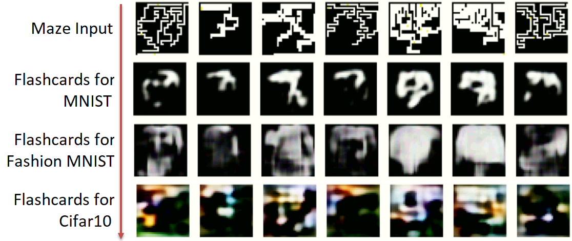
Figure 3: Transformation from maze patterns into Flashcards for different tasks: MNIST, Fashion MNIST and Cifar10.

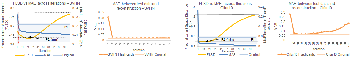
Figure 4: Analysis on $r$ for flashcards construction, demonstrated using SVHN and Cifar10. Odd columns portray metrics corresponding to change on passing multiple random maze inputs in iterative fashion through an AE. Orange curve depicts the trend of Fréchet latent space distance (FLSD) between intermediate input at (t) iteration and original data samples, dark blue curve shows constant decrease in reconstruction error between (t-1) and (t), across different iterations for each dataset. Light blue line serves as reference MAE on original data. Property P1 is satisfied when the blue curve goes below $\epsilon_{1}$ (marked by dotted red line) and P2 is satisfied at the first minima of FLSD, which occurs around $10\leq r\leq 20$, irrespective of dataset. Even columns compare AE error (MAE) between test data and its reconstruction, when trained on flashcards constructed from different iterations. This again confirms the acceptable range of $r$ and that flashcards construction is not critically sensitive to the choice of $r$ within the range.

Let $\mathbf{F}_{ri}$ be the output after a series of $r$ recursive iterations/passes of $\mathbf{M}_{i}$ through the trained AE ($f_{t}(\cdot,{\boldsymbol{\theta}}_{t})$), i.e.,

$$\mathbf{F}_{ri}=f_{t}^{r}(f_{t}^{r-1}(\cdots f_{t}^{1}(\mathbf{M}_{i},{{{\boldsymbol{\theta}}_{t}}})\cdots)).$$ (4)

Such recursive passing (output $\rightarrow$ input $\rightarrow$ output) gradually attunes the input to ${\boldsymbol{\theta}}_{t}$. This can be observed in Figure 2 where the MAE reduces over recursive iterations, and the latent space representations of samples drawn from $P(\mathbf{M})$ increasingly overlap with those from $P(\mathbf{X})$. Let

$$\gamma_{1}\leq|\mathbf{F}_{ri}-\mathbf{F}_{(r-1)i}|\leq\gamma_{2},~{}\forall\mathbf{M}_{i}\in D_{m}\sim P(\mathbf{M}),$$ (5)

where $\gamma_{1}$, and $\gamma_{2}$ are the lower and upper bounds of reconstruction error for any $\mathbf{M}_{i}\in D_{m}$. The aim now is to have a collection set $F_{t}=\{\mathbf{F}_{ri}:i=1,\ldots,N_{f}\}$ for task $T_{t}$ such that the following properties are satisfied:

• P1: $\gamma_{2}<\epsilon_{1}$ for $\forall\mathbf{M}_{i}\in D_{m}$,

• P2: The latent space distribution of $F_{t}\sim D_{t}$, i.e. $~{}D_{m}\rightarrow D_{t}$.

Such a set of constructions ($F_{t}$) obtained through recursive iterations of random inputs (drawn from $P(\mathbf{M})$) are defined as flashcards. Such constructed flashcards are expected to capture the knowledge from the trained network and serve as a potential alternative to $D_{t}$. Figure 3 illustrates a few flashcards constructed with same set of random images, from AEs trained with different datasets. Although these flashcards are intended to capture the knowledge representations in ${{{\boldsymbol{\theta}}_{t}}}$ as a function of $\mathbf{M}_{i}\in D_{m}$, it can be observed from Figure 3 that they do not bear direct shape similarities with their respective datasets. In fact, during the recursive process, the raw input image patterns are modified/transformed to textures that are suited to the trained AE model. This is in-line with (Geirhos et al., 2019) which shows that neural networks learn predominantly texture than shape by default. Now, since an AE is trained to maximize $\log P(\mathbf{X}|{{{\boldsymbol{\theta}}_{t}}})$, the following fact holds:

Fact 1:

Let $D_{A}$ and $D_{B}$ be two i.i.d. datasets whose elements are drawn from $P(\mathbf{X})$. If there exists a trained AE $f_{A}(\cdot,{\boldsymbol{\theta}}_{A})$, to reconstruct $D_{A}$ with error $[\beta_{1},\beta_{2}]$, $\forall\mathbf{X}\in D_{A}$, then the AE $f_{A}(\cdot,{\boldsymbol{\theta}}_{A})$ can reconstruct $D_{B}$ with the same error range.

The converse is not true because any image dataset $D_{B}$ with images that have few pixels with non-zero values (other pixels as zeros), can still yield smaller reconstruction error and not necessary to be drawn from $P(\mathbf{X})$ (satisfying P1). Hence, both P1 and P2 for $F_{t}$ need to be satisfied. As P1 and P2 are dependent on the initial input distribution $P(\mathbf{M})$, it is important to have a suitable $P(\mathbf{M})$ to get $F_{t}$ ($P(\mathbf{M})=P(\mathbf{X})$ is one trivial and uninteresting solution). As finding a perfect $P(\mathbf{M})$ is an ideal research problem by itself, in this work, we use random maze pattern images as a potential candidate $D_{m}$ to get $F_{t}$. The above leads to the following hypothesis:

Hypothesis 1:

Since the AE trained on $D_{t}$ also reconstructs elements from $F_{t}$ (Property P1) and has matching latent space distribution (Property P2), flashcards ($F_{t}$) can be used as a set of pseudo-samples for $D_{t}$ to learn $f_{t}(\cdot,{{{\boldsymbol{\theta}}_{t}}})$, when trained from scratch using only $F_{t}$.

2.1 Flashcard Construction

Algorithm 1 Flashcard construction

0:  $f_{t}(\cdot,{\boldsymbol{\theta}}_{t})$: AE model for task $T_{t}$

0:  $N_{f}$: Number of flashcards

0:  $r$: Number of recursive iterations through $f_{t}(\cdot,{\boldsymbol{\theta}}_{t})$at

1:  Let $D_{m}\leftarrow\left\{\mathbf{M}_{1},\ldots\mathbf{M}_{N_{f}}\right\}$, where $\mathbf{M}_{i}\sim P(\mathbf{M}),\forall i$, $P(\mathbf{M})$ corresponds to the distribution of initial input patterns

2:  $F_{t}\leftarrow\{\}$, where $F_{t}$ denotes the set of flashcards

3:  for $i\in\left\{1,\ldots,N_{f}\right\}$ do

4:     $\mathbf{F}_{ri}=f_{t}^{r}(f_{t}^{r-1}(\cdots f_{t}^{1}(\mathbf{M}_{i},{{{\boldsymbol{\theta}}_{t}}})\cdots))$

5:     $F_{t}=F_{t}\cup\{\mathbf{F}_{ri}\}$

6:  end for

7:  return  $F_{t}$

Algorithm 1 provides the steps to construct flashcards using a trained AE model. For flashcards construction, the following hyperparameters are useful - (i) number of recursive iterations ($r$), (ii) number of flashcards to construct ($N_{f}$), (iii) choice of initial input distribution ($P(\mathbf{M})$). Figure 4 portrays empirical analysis of selecting the optimal iteration, considering complex (with background) datasets such as SVHN and Cifar10 dataset. Figure 4 (columns 1,3) shows Frechet Latent Space Distance (FLSD is inspired from FID (Heusel et al., 2017) and calculated as the Frechet distance between latent space activations of flashcards versus original samples (smaller the better), from the eyes of the trained AE) (Orange) and MAE (Blue), as a function of $r$. Initially, increase in $r$ leads to decrease in FLSD, up to certain iterations, this indicates that flashcards distribution is getting closer to learned distribution. As $r$ increases further, though MAE keeps going down, FLSD increases, because propagation of reconstruction error in AE causes drift in the features. Based on the empirical analysis $10\leq r\leq 20$ is a sensible choice that worked well across all of our experiments. Also, reconstruction error (Figure 4, columns 2,4) is observed to be low in this iteration range. It further indicates that the flashcards are not critically sensitive to $r$. Hence, in all the experiments we set $r$ to be 10.

Dataset	Original MAE	Flash-cards MAE	Alpha on Original	Alpha on Flashcards	Alpha on Untrained
MNIST	$0.0184$	$0.0491$	$1.9185$	$2.0531$	1.4343
Fashion	$0.0259$	$0.0440$	$2.0044$	$2.1158$	1.4343
Cifar10	$0.0564$	$0.0686$	$2.0266$	$2.1531$	1.4343

Table 1: Reconstructions from two separate AE, first trained on original data, and second trained on flashcards.The metrics indicate that flashcards are sufficient alternatives towards learning the particular data. Weighted Alpha (Martin and Mahoney, 2020) is based on HT-SR Theory. Alpha values are closer for the trained networks which indicates similarity between the two network weights. Reported values are obtained by taking mean over 5 runs.

Train Arch. Type	Params	Test on Original	Test on AE1	Test on AE2
AE1 - Variant I	$94,243$	$0.0640$	$0.0725$	$-$
AE2 - Smaller arch.	$24,083$	$0.0787$	$0.0939$	$0.0963$
AE2 - Larger arch.	$372,803$	$0.0512$	$0.0681$	$0.0570$
AE1 - Variant II	$298,947$	$0.0437$	$0.0599$	$-$
AE2 - Smaller arch.	$24,083$	$0.0358$	$0.0385$	$0.0389$
AE2 - Larger arch.	$372,803$	$0.0512$	$0.0654$	$0.0570$

Table 2: Building autoencoder AE2 using flashcards obtained from AE1 (two variants) trained on Cifar10 dataset. Columns AE1 and AE2 refer to test MAE on Cifar10 when flashcards obtained from AE1 and AE2 are used to train for reconstruction, respectively. Better performance on AE2 Smaller using flashcards from AE1 shows transferability using existing flashcards.

In general, as more flashcards are introduced, performance gets better. In our experiments, number of flashcards constructed equals the same no. of samples in original data. Note from (Ostapenko et al., 2019), that memory requirement is calculated based on network parameters and is independent of generated samples.

As mentioned above, the choice of $P(\mathbf{M})$ is the maze-like random image patterns that resembles edges and shapes. Gaussian random noise (pixel-wise & geometric patterns) were also considered and it was observed that pixel-wise noise does not help in capturing representations, and maze patterns outperformed geometric patterns.

2.2 Flashcards for Capturing Representations

We first verify Hypothesis 1 by demonstrating the efficacy of flashcards to capture representations on single-task scenario (Algorithm in Supplementary).

Alternative to Original Dataset: Consider three different datasets: MNIST, Fashion MNIST, and Cifar10. Let 3 autoencoders AE1, AE2, AE3 (all with same architecture) be trained for each of these 3 datasets separately using Eqn. (1) as loss function. Flashcards ($F_{t}$) constructed from each of these AEs, for the same set of random input maze pattern images ($D_{m}$) (few samples shown in Figure 3) are used respectively to train new AE models from scratch (with the same architecture), namely AE-flash1, AE-flash2, and AE-flash3. Results in Table 1 show reconstructions are very close to AE trained on original. These results confirm the hypothesis that flashcards indeed capture network parameters as a function of $D_{m}$, therefore be used as pseudo-samples / training data (as network parameters involved in flashcard construction are initially learned by training with the original dataset $D_{t}$).

Knowledge Distillation to smaller/larger architecture: Consider training a network AE1 with a certain data $D_{T_{1}}$. Once trained, $D_{T_{1}}$ may not be available because of confidentiality/privacy, storage requirements, etc. In regular KD, this creates a bottleneck because original data is still required to be shown to the new network. If in the future, there is a newer and better architecture AE2, our method enables migration by training on flashcards constructed from AE1. We show this is possible by training two network variants - one smaller and one larger modified architectures than original (Table 2).

2.3 Flashcards for Replay in CL

Consider a sequence of $T$ tasks {$T_{1},\ldots,T_{t},\ldots,T_{T}$}. In the CL scenario, the AE for task $T_{t+1}$ is required to be trained on top of previous learned tasks $T_{1},\ldots,T_{t}$. In other words, ${{{\boldsymbol{\theta}}_{t+1}}}$ is adapted from the previously trained network parameters ${{{\boldsymbol{\theta}}_{t}}}$. Such AE training for task $T_{t+1}$ may result in AE forgetting the representations learned till the previous task $T_{t}$. Unlike other CL based approaches which aims to preserve ${{{\boldsymbol{\theta}}_{t}}}$ through regularization, memory replay (either episodic or using external generative networks), architectural strategies, or their combinations, we use the flashcards constructed on ${{{\boldsymbol{\theta}}_{t}}}$ along with data for task $T_{t+1}$, while training for task $T_{t}$. Flashcards are required to be constructed only at the end of task $T_{t}$ irrespective of the number of preceding tasks, so that knowledge representations for tasks $\{1,\ldots,t\}$ can be captured and trained with the next task $T_{t+1}$. Thus, the proposed method avoids storing of flashcards for each successive task, thereby significantly reducing the memory overhead, while ensuring robust performance (Section 4. Algorithm 2 provides the steps for using flashcards as a replay strategy for CL. In our CL experiments, flashcards 10% (of next task samples) were constructed on-the-fly before training a new task (irrespective of number of previous tasks). Increasing this number helps to remember previous tasks better.

Algorithm 2 Flashcard for Replay in CL

0:  $f_{t}(\cdot,{\boldsymbol{\theta}}_{t})$: AE model for task $T_{t}$; $N_{f}$: Number of flashcards; $r$: Number of iterations through $f_{t}(\cdot,{\boldsymbol{\theta}}_{t})$

0:  $D_{t+1}$: Data for task $T_{t+1}$

1:  $F_{t}\leftarrow$ Algorithm 1 ($f_{t}(\cdot,{\boldsymbol{\theta}}_{t}),N_{f},r$), where $F_{t}$ is the set of flashcards for task $T_{t}$

2:  Train the autoencoder model $f_{t+1}(.,{\boldsymbol{\theta}}_{t+1})$ on flashcards $F_{t}$ and data $D_{t+1}$

3:  Initialize ${\boldsymbol{\theta}}_{t+1}\leftarrow{\boldsymbol{\theta}}_{t}$

4:  Optimize ${\boldsymbol{\theta}}_{t+1}$ using given loss

$${\boldsymbol{\theta}}_{t+1}^{*}\leftarrow\operatorname*{arg\,min}_{{\boldsymbol{\theta}}_{t+1}}{\big{(}}\frac{1}{|D_{t+1}|}\sum_{n=1}^{|D_{t+1}|}|D_{t+1}^{(n)}-f_{t+1}(D_{t+1}^{(n)},{\boldsymbol{\theta}}_{t+1})|$$

$$+\frac{\lambda}{N_{f}}\sum_{n=1}^{N_{f}}|F_{t}^{(n)}-f_{t+1}(F_{t}^{(n)},{\boldsymbol{\theta}}_{t+1})|{\big{)}}$$

5:  return  $f_{t+1}(.,{\boldsymbol{\theta}}_{t+1}^{*})$

3 Related Works

In general, CL algorithms are based on architectural strategies, regularization, memory replay, and their combinations (Parisi et al., 2019). By the intrinsic nature of flashcards (as discussed in Sections 2.2 and 2.3), they implicitly exhibit the characteristics of both regularization (refer Algorithm 2 point 4) and replay, and will therefore be compared with the respective CL strategies.

Regularization strategies such as (Kirkpatrick et al., 2017), (Zenke et al., 2017) learn new tasks while imposing constraints on the network parameters to avoid straying too much from those learned from the previous tasks. (Li and Hoiem, 2018) uses current task samples to regularize the soft labels of past tasks, thus avoiding explicit data storage. However, it is important to note that these regularization methods perform well in homogeneous task environments, where it is possible to find mutually sub-optimal points in the solution space. However, such methods suffer when subsequent tasks are from different domains / heterogeneous datasets (also reported in (Li and Hoiem, 2018)).

In a rehearsal mechanism, subset of samples from previous tasks, referred to as coreset samples / exemplars, serve as memory replay (Lopez-Paz and Ranzato, 2017), (Chaudhry et al., 2019), (Castro et al., 2018). However, they suffer from excessive storage requirements that grows with the number of tasks. On the other hand, generative replay approaches (van de Ven et al., 2020), (Rostami et al., 2020), (Aljundi et al., 2019), (Li et al., 2020) face challenges in scalability to complicated problems with many tasks, since they involve heavy training and computation associated with an auxiliary network to generate visually meaningful images for each task.

Approaches discussed above are either suitable only for homogeneous data, or are memory intensive as they involve preserving samples, or computationally intensive in ”generating” samples, or requiring task identifiers. The proposed flashcards based capturing of learned representations are constructed on the fly, requires only simple autoencoder, independent of the no. of tasks, and helpful both as regularization and replay mechanism. Flashcards can be used as pseudo samples constructed with low computational and memory expense. Furthermore, flashcards can scale across tasks without considerable drop in performance. Some main characteristics of flashcards against other replay based CL approaches are summarized in Table 1 of Supplementary.

4 Experiments in Continual Learning

We provide experimental validation of using flashcards in CL scenario as replay for variety of different applications such as: (i) continual reconstruction (Section 4.1), (ii) continual denoising (Section 4.2), and continual classification (Section 4.3), split into Task Incremental Learning (Task-IL) and New Instance Learning (NIL). For the first two experiments, we use 5 heterogeneous public datasets (referred as Sequence5), namely MNIST, Fashion MNIST, Cifar10, SVHN, and Omniglot. For Task-IL classification, we use Sequence3 comprising of Cifar10, MNIST and Fashion MNIST. For NIL classification, we use Cifar10.

For reconstruction, denoising and NIL classification, flashcards are constructed using an AE architecture with 4 layers of down/upsampling and 64 conv filters per layer. The bottleneck dim 256 is 12x reduction from image space, and serves to demonstrate effectively the forgetting in CL. The architecture is a simplified variant of the VGG style , adapted with lesser layers and filters to enable proper reconstruction for the baseline. All hidden layers employ tanh activation. The network is trained for 100 epochs per task, and optimized using Adam with a fixed learning rate of 1e-3. Each minibatch update is based on equal number of flashcards and the current task samples. 10% of the training data is allocated for validation. Early stopping is employed if there is no improvement for over 20 epochs. 5K flashcards with $\lambda=1$ was used as replay for reconstruction and denoising. The workstation used for training has 64GB RAM and NVIDIA RTX Titan GPU. For all experiments, we compare with upperbound (Joint Training), lowerbound (Sequential Fine-tuning, SFT), and examples of methods using regularization, generative and episodic replay as baseline.

Method	Type	Nw. (MB)	Mem. (MB)	Recon MAE	Recon BWT	Denoise MAE	Denoise BWT
JT	-	1.5	798.7	$0.035$	-	$0.055$	-
SFT	-	1.5	-	$0.552$	$-0.64$	$0.547$	$-0.63$
Coreset 500	ER	1.5	1.5	$0.058$	$-0.02$	$0.075$	$-0.02$
Coreset 5K	ER	1.5	15.4	$0.049$	$-0.02$	$0.059$	$-0.02$
LwF	Reg	1.5	-	$0.549$	$-0.52$	$0.437$	$-0.33$
VAE-5K+AE	GR	2.9	-	$0.075$	$-0.06$	$0.071$	$-0.04$
CL-VAE 5K	GR	1.4	-	$0.352$	$-0.16$	$0.546$	$-0.28$
Flashcards5K	FR	$\mathbf{1.5}$	-	$\mathbf{0.053}$	$\mathbf{-0.03}$	$\mathbf{0.058}$	$\mathbf{-0.03}$

Table 3: Continual learning for reconstruction and denoising (added standard noise of 0.1), values averaged over 5 runs (stdev in Supplementary). Comparison in terms of average error (MAE), forgetting (BWT), Network Capacity (Nw. (MB)) and External Memory (Mem. (MB)) is presented. Flashcards performs better than generative replay, and is on-par with episodic memory (coreset), without need for external memory. Reg=Regularization, ER=Episodic Replay, GR=Generative Replay, FR=Flashcard Replay.

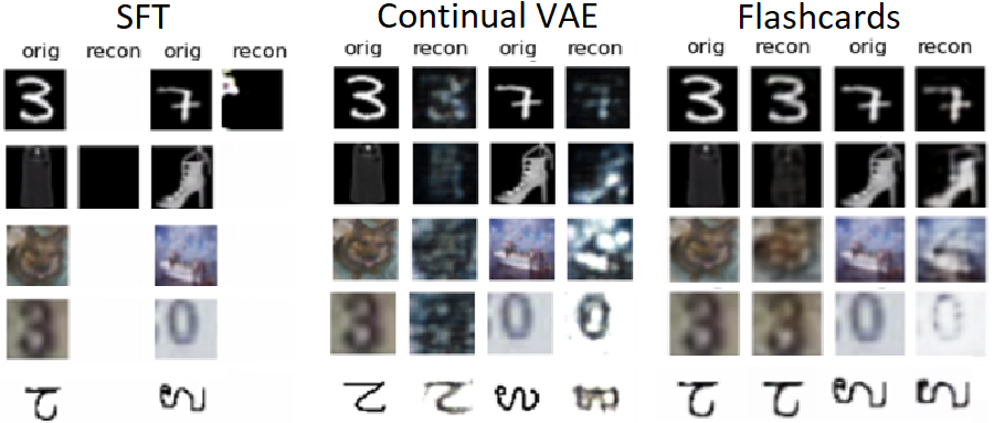
Figure 5: Comparison between different methods for continual reconstruction using Sequence5. The figure shows the impact of forgetting after the end of the last task, i.e. Omniglot (all intermediate results are in Supplementary). Each row presents a dataset/task. Sequential Fine Tuning (SFT, left), is not able to reconstruct, even when presented with Omniglot, because (i) catastrophic forgetting and (ii) unsuitable transfer learned weight initialization. Continual VAE (center) fares better but has artifacts and color loss in the reconstructions. Flashcards (right) remembers all previous tasks.

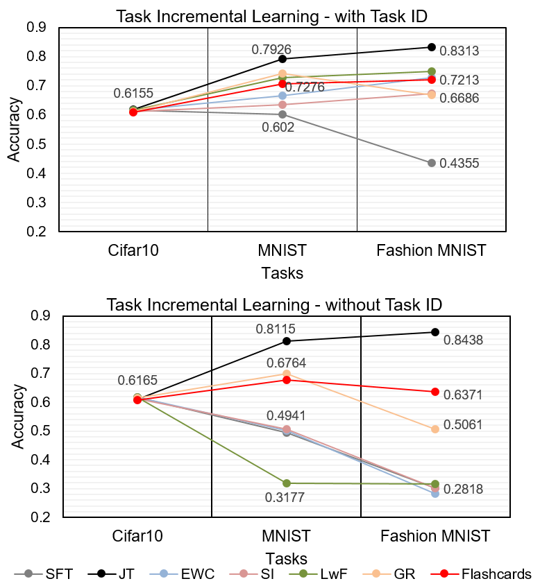
Figure 6: Comparison of different methods for task incremental learning using Sequence3 tasks (Cifar10-MNIST-FashionMNIST). When task id is provided, flashcards performs similar to baseline methods. However, baselines fail in absence of identifier. Flashcards is robust to degradation across different domain tasks and outperforms other methods. Comparison: upperbound (JT), lowerbound (SFT), EWC, SI, LwF and Generative Replay with VAE (GR) accuracy. Results are averaged over 5 runs.

4.1 Continual Reconstruction

Sequence5 is used to demonstrate reconstruction in CL. We measure individual task MAE and BWT (Lopez-Paz and Ranzato, 2017), customized for reconstruction. Results are listed in Table 3 and visualized in Figure 5. Comparison with baseline is summarized in the captions for ease of convenience. To the best of our knowledge, we are the first to report continual reconstruction. We compare flashcards against different replay and regularization techniques and observe it outperforms most baselines and on-par with episodic replay. Results for permutations of Seq3 (MNIST-Fashion-Cifar10) in Suppl.

4.2 Continual Denoising

A more challenging extension to traditional AE reconstruction is denoising. We impose noise sampled from a standard normal distribution factored by 0.1 to Sequence5, and expect the network to denoise it. To the best of our knowledge, we are the first to report Continual Denoising. Results reported for Denoise MAE and BWT in Table 3 are obtained by adding noise factor of 0.1 to original images. Flashcards perform better compared to baseline approaches. More visual results for different noise levels are provided in Supplementary.

4.3 New Task Classification

Task Incremental Learning (Task-IL) assumes learning new tasks, each comprising of multiple classes ($\geq 2$). The encoder is shared with task-exclusive multihead output. Generally, classification is performed using the specific multihead, with the help of task identifier. Baseline methods built specifically in this setup perform poorly in absence of task ID (see Figure 6). We compare performance of flashcards for both cases, with and without task ID. We follow the same setup as provided in (van de Ven et al., 2020), replacing the last dense layer with 128 neurons instead of 2000. For the first task, classifier is trained normally. AE’s encoder for flashcard construction shares same architecture as classifier encoder, and is pre-initialized with its weights, and allowed to train fully along with additional decoder. Successive tasks for both networks use new samples along with the constructed flashcards, trained for 5000 iterations, optimized using Adam with lr=0.0001, and batch size of 256. Both class soft-scores and latent space regularization is applied to classifier on replay of flashcards ($\lambda=1$). In Figure 6, flashcards is stable with and without task ID and further beats other baseline methods in the absence of task id. Network arch. in Supplementary.

4.4 New Instance Classification

Single Task, New-Instance Learning (ST-NIL) classification introduced by (Lomonaco and Maltoni, 2017), focuses on learning new instances every session while retaining the same number of classes. Performance indicates how well the model adapts to virtual concept drift across sessions. Flashcards are constructed from AE (unsupervised) per session and passed to the classifier to get predicted softmax scores as soft class-labels. It is observed that flashcards’ performance is better than regularization and on-par with episodic replay, without explicitly storing exemplars in memory. (Table 4). ResNet18 is used as classifier, optimized using SGD with learning rates of 0.001 over 20 epochs, and new sessions are introduced by adopting the same brightness and saturation from (Tao et al., 2020), test set is constant across sessions.

Session/ Method	Type	1	2	3	4	5
Naive*	-	$67.80$	$69.31$	$71.37$	$73.12$	$73.23$
Cumulative*	-	$67.80$	$76.13$	$81.22$	$81.83$	$82.12$
EWC*	Reg	$67.80$	$69.45$	$72.68$	$74.02$	$74.31$
SI*	Reg	$67.80$	$70.48$	$72.82$	$74.63$	$74.58$
IMM*	Reg	$67.80$	$69.69$	$72.85$	$74.37$	$73.84$
EEIL 1K*	ER	$67.80$	$71.97$	$73.27$	$\mathbf{74.91}$	$74.66$
A-GEM 1K*	ER	$67.80$	$\mathbf{72.27}$	$\mathbf{73.72}$	$74.81$	$\mathbf{75.15}$
Flashcards1K	FR	$67.90$	$71.40$	$73.34$	$74.84$	$74.88$

Table 4: ST-NIL Classification on Cifar10 using the settings described in (Tao et al., 2020). * are reported from the same paper. Flashcards created from unsupervised AE performs equally well in comparison to other methods primarily built for classification. Reg=Regularization, ER=Episodic Replay, FR=Flashcard Replay.

5 Conclusion

We introduced flashcards that can capture knowledge representations of a trained AE through recursive passing of random image patterns, and showed that it can be used as alternative to original data. We further demonstrated its efficacy as a task agnostic replay mechanism for various CL scenarios, such as classification, denoising, task incremental learning, with heterogeneous datasets. Flashcard replay outperforms generative replay and regularization methods, without additional memory and training, and also performs on par with episodic replay, without storing exemplars. The intrinsic nature of flashcards allows for data abstraction which can be exploited for data privacy applications. Generalization of flashcards to other domains will foster further research.

Appendix A Datasets

The datasets used in Sequence5 are in the order - MNIST, Fashion MNIST, Cifar10, SVHN, and Omniglot. Each dataset was considered as a task, and class labels were omitted. MNIST, Fashion MNIST and Omniglot were resized to 32x32x3 (bilinear rescale and channel copied twice) to maintain the same scale as the other two datasets.

Appendix B Flashcards for Single-Task Scenario

Algorithm 3 provides the steps to use flashcards for single-task scenario.

Algorithm 3 Flashcard for Single-Task / General Scenario

0:  $f_{t}(\cdot,{\boldsymbol{\theta}}_{t})$: AE model for task $T_{t}$

0:  $N_{f}$: Number of flashcards

0:  $r$: Number of iterations through $f_{t}(\cdot,{\boldsymbol{\theta}}_{t})$

1:  $F_{t}\leftarrow$ Algorithm 1 ($f_{t}(\cdot,\boldsymbol{\theta}_{t}),N_{f},r$), where $F_{t}$ is the set of flashcards for task $T_{t}$

2:  Train a new AE model $g_{t}(.,{\boldsymbol{\phi}}_{t})$ on Flashcards $F_{t}$,

$${\boldsymbol{\phi}}_{t}^{*}\leftarrow\operatorname*{arg\,min}_{\phi_{t}}\frac{1}{N_{f}}\sum_{n=1}^{N_{f}}|F_{t}^{(n)}-g_{t}(F_{t}^{(n)},{\boldsymbol{\phi}}_{t})|,$$

where $F_{t}^{(n)}$ is the $n^{th}$ flashcard sample

3:  return  $g_{t}(.,{\boldsymbol{\phi}}_{t}^{*})$

Appendix C Comparison between Flashcards and other Replay methods

Table 5 provides detailed comparison between Flashcards and other replay strategies such as episodic memory and generative replay.

Appendix D Benchmarking Flashcards Number of Samples

Increase in flashcards number shows improvement - examples for MNIST and Cifar10, as observed in Figure 7. Trend followed by flashcards is similar to the improvement shown with increasing coreset/exemplars.

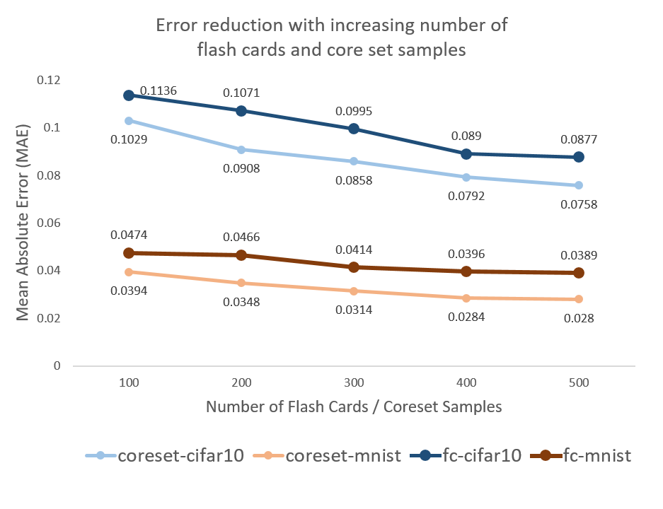
Figure 7: Increase in no. of flashcards / coreset improves performance - Quantitative error reduction in (i) Cifar10, (ii) MNIST.

Trait	Flashcards for Replay	Episodic Memory Replay	Generative (Data) Replay
Examples
Single-Task Scenario
Alternative to original data?	Yes	No, subset of original	Yes
Distinction	Postprocess knowledge capture from trained network	Stores a subset of the original data in memory	Network is trained to generate samples per task
Visually similar to dataset?	No	Yes	Depends on complexity
Performance on task	Close to original network	Very close to original network	Close to original network
Continual Learning Scenario
Store sample across tasks?	No	Yes, need to store per task	Depends on nw. complexity
Nw. used to obtain alt. data	Simple AE	N/A	VAE / GAN etc.
Allocate extra memory between each task?	No, just in time creation during next task	Yes, either memory or disk	Depends on network’s inbuilt support for CL
Constructed on the fly?	Yes, just before starting next task training	No, store original samples in memory	On the fly (if CL supported) or each task’s exclusive nw.
Independent of no. of tasks?	Yes, only need samples from current snapshot	No, need to store per task	Depends on network’s inbuilt support for CL
Scaling up tasks in number and complexity	Empirical results shows strong feasibility	Straightforward; requires linear memory storage	Scaling up in terms of no. of tasks is challenging

Table 5: Comparison between three major replay techniques.

Appendix E Using Flashcards Representation for Downstream Classification

Dataset	Original	Classifier 1	Classifier 2
MNIST	$0.9940$	$0.9921$	$0.9869$
Fashion MNIST	$0.9215$	$0.9126$	$0.8978$
Cifar10	$0.8003$	$0.6295$	$0.5659$

Table 6: Building a classifier using the reconstructions from flashcard trained network. Reported accuracy averaged over 5 runs. Cifar10 accuracy is lower due to relatively higher AE recon error.

Let AE1 be trained on original images $D_{T_{1}}$ and AE-Flash1 be trained using flashcards $D_{f_{1}}$ from AE1. Let the respective reconstructions (after training) be $\widehat{D_{T_{1}}}$ and $\widehat{D_{F_{1}}}$. Next, train two classifiers (VGG16), Classifier1 and Classifier2 using $\widehat{D_{T_{1}}}$ and $\widehat{D_{F_{1}}}$, respectively, and compare their performance on independent test set of original images. The results tabulated in Table 6 shows that flashcards based networks are also capable of performing reasonably well in downstream tasks such as classification.

Appendix F AutoEncoder Architecture Selection

We train several AE architectures on Cifar10 dataset to compare the performance of flashcards for reconstruction. Table 7 provides the details about various model architectures and the corresponding test Mean Absolute Error (MAE) on training using the original dataset (Original MAE) and using Flashcards generated from the trained AE (Flashcards MAE), respectively.

We choose the architecture Blk_4_fil_64 for all our experiments for reconstruction and denoising tasks. Blk_4_fil_64 architecture obtains $0.0512$ Original MAE and $0.0570$ Flashcards MAE. Blk_3_fil_64 and Blk_2_fil_32 achieve better Original MAE/Flashcards MAE than Blk_4_fil_64, but both these architectures use higher latent space size ($1024$ and $2048$). The improvement in reconstruction MAE may be attributed to such high latent space dimensions which might not encode useful information and just act as a copy function. Hence, we choose the Blk_4_fil_64 architecture.

Arch. Type	Model Params.	Latent Space	Num. Blocks	Num. Filters	Original MAE	Flashcards MAE
Blk_4_fil_16	$24,083$	$64$ (48x reduction)	$4$	$16$	$0.0787\pm 0.0002$	$0.0963\pm 0.0004$
Blk_4_fil_32	$94,243$	$128$ (24x reduction)	$4$	$32$	$0.0640\pm 0.0002$	$0.0725\pm 0.0009$
Blk_4_fil_64	$372,803$	256 (12x reduction)	$4$	$64$	$0.0512\pm 0.0004$	$0.0570\pm 0.0006$
Blk_4_fil_128	$1,482,883$	$512$ (6x reduction)	$4$	$128$	$0.2062\pm 0.0000$	$0.2445\pm 0.0476$
Blk_3_fil_64	$298,947$	$1024$ (3x reduction)	$3$	$64$	$0.0437\pm 0.0003$	$0.0599\pm 0.0067$
Blk_2_fil_32	$57,251$	$2048$ (1.5x reduction)	$2$	$32$	$0.0358\pm 0.0008$	$0.0389\pm 0.0015$

Table 7: Architecture selection for AutoEncoder (AE). We train several AE architectures on Cifar10 dataset in order to compare the performance of flashcards for reconstruction. Various details about the architecture such as Model Params. (Number of trainable weights and biases), Latent Space (Size of latent space/bottleneck layer and its reduction rate versus image space), Num. Blocks (Number of convolution + pooling blocks in Encoder), and Num. Filters (Number of filters in convolution layers) are also provided. Original MAE is the Cifar10 test MAE on AE trained using Cifar10 train dataset. Flashcards MAE is the Cifar10 test MAE on AE trained using the flashcards obtained from given AE. The reported standard deviation for the scores are obtained over 5 experimental runs.

Appendix G Redefining Metrics for Reconstruction

We measure individual task MAE before and after observing the data for the given task as well as the ability of transferring knowledge from one task to another, by measuring BWT (Backward Transfer) and FWT (Forward Transfer). We follow the similar definition for avg mean absolute error (MAE), BWT, and FWT as described in [Lopez-Paz and Ranzato, 2017]. It must be noted that [Lopez-Paz and Ranzato, 2017] describes these definitions in a supervised setting. As we explore an unsupervised representation, we redefine these metrics for unsupervised settings. Consider we have the test sets for each of the $T$ tasks. We evaluate the model obtained after training task $T_{t}$ on all $T$ tasks. This gives us the matrix $M\in R^{{T\times T}}$, where $M_{i,j}$ represents the test MAE for model on task $T_{j}$ after observing the data of task $T_{i}$. Let $r$ be vector of test MAEs for each task obtained using random weight initializations. Then, we define following three metrics,

$$AvgMAE=\frac{1}{T}\sum\limits_{i=1}^{T}M_{T,i}$$ (6)

$$BWT=\frac{1}{T-1}\sum\limits_{i=1}^{T-1}(M_{i,i}-M_{T,i})$$ (7)

$$FWT=\frac{1}{T-1}\sum\limits_{i=2}^{T}(r_{i}-M_{i-1,i})$$ (8)

Lower value for Avg MAE and higher values for BWT and FWT are better.

Appendix H Sequence5 Continual Reconstruction

We provide visuals for each task in Sequence5 showing how each method handles forgetting. Figure 8 shows Sequential Fine Tuning (SFT) is the naive approach and suffers the most. It can be observed that reconstructions are empty, this is because of the network parameters at the start of task 5, which prevents it to learn the current Omniglot task itself. Figure 9 shows the effect of replay with 500 real samples (coreset). 500 samples were chosen as their memory matches the AE network parameters of 1.5MB. From the experimental results, it is observed that 500 samples are not sufficient to beat flashcards. Figure 13 has individual graphs for different methods show the variation of test Mean Absolute Error (MAE) on current task dataset after observing the data for sequence of tasks.

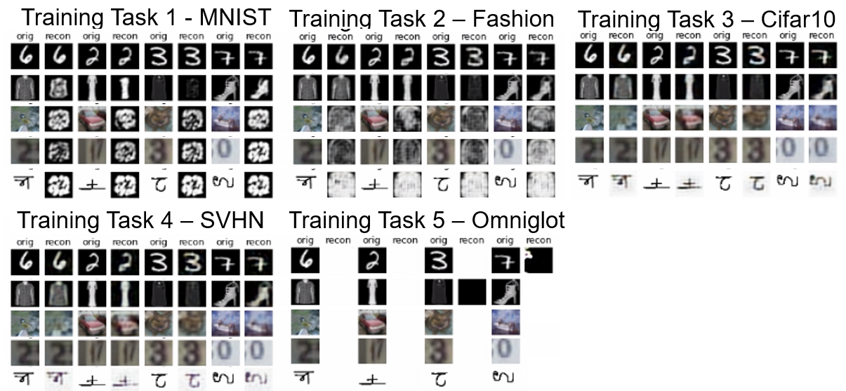
Figure 8: Continual Reconstruction on Naive / Sequential Fine Tuning (SFT).

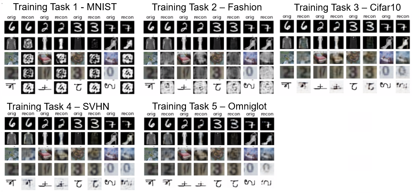
Figure 9: Continual Reconstruction using episodic memory - coreset 500.

Figure 10 is based on VAE trained in CL fashion, maintaining the same mean and std.dev. across tasks. It is not sufficient to mitigate forgetting.

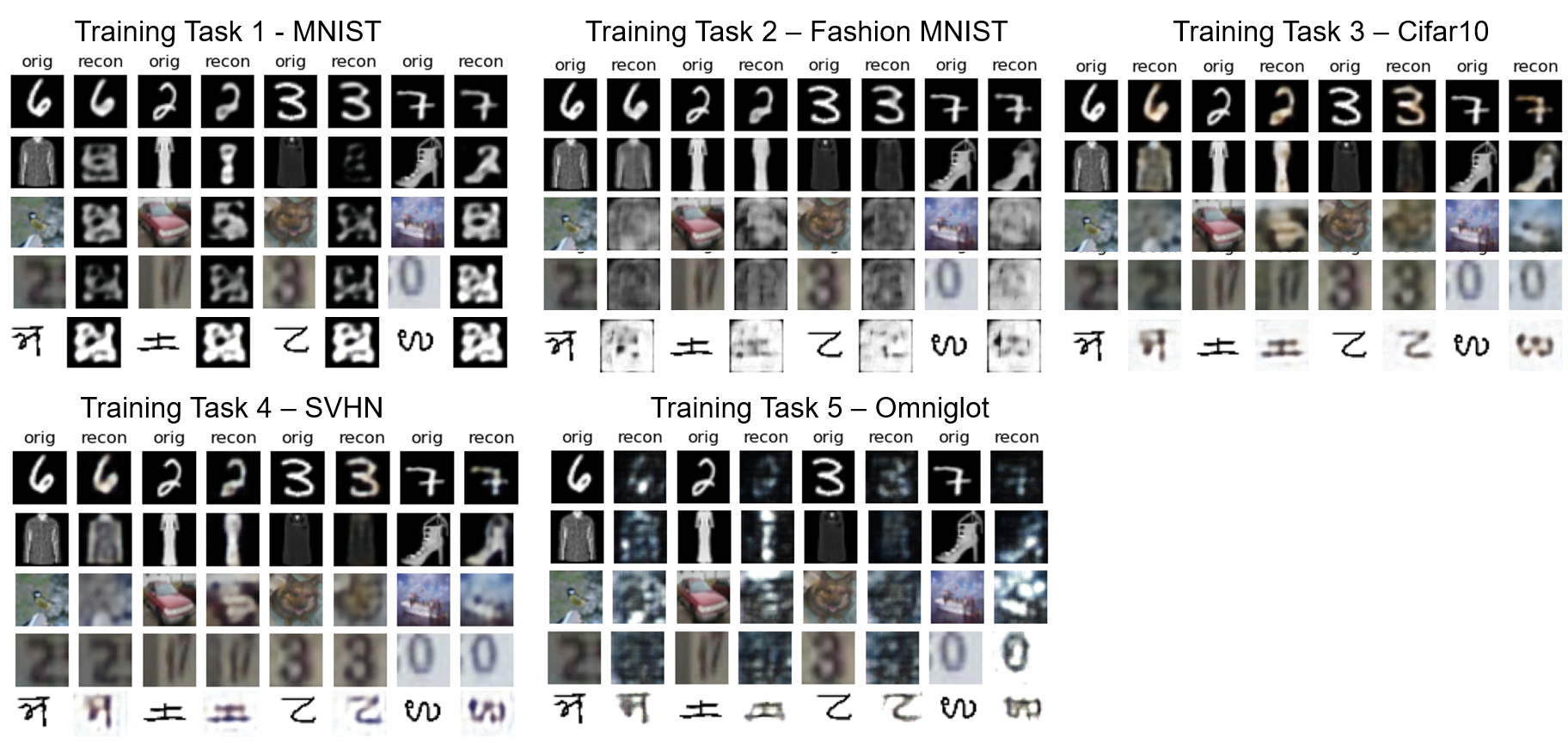
Figure 10: Continual Reconstruction using VAE trained exlusively for Continual Learning.

Figure 11 uses AE for reconstruction supplemented by an external VAE for generative replay. Though results are competitive with Flashcards, there is still forgetting in the previous tasks - MNIST and Fashion MNIST.

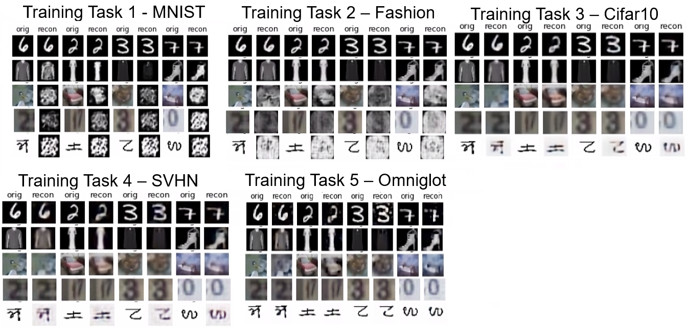
Figure 11: Continual Reconstruction using AE + VAE as generative replay.

Figure 12 presents results when using Flashcards, where the past and current task samples are remembered well.

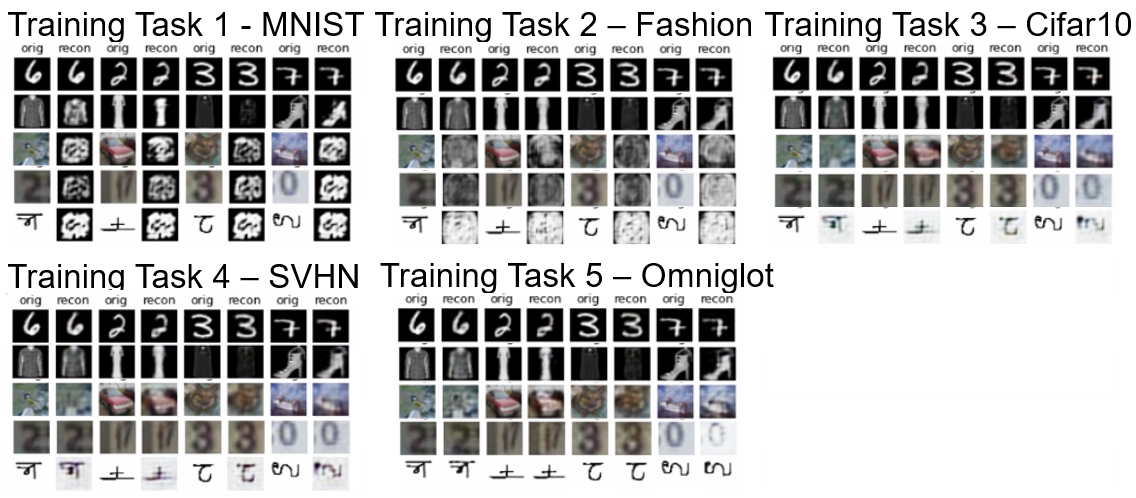
Figure 12: Continual Reconstruction using Flashcards.

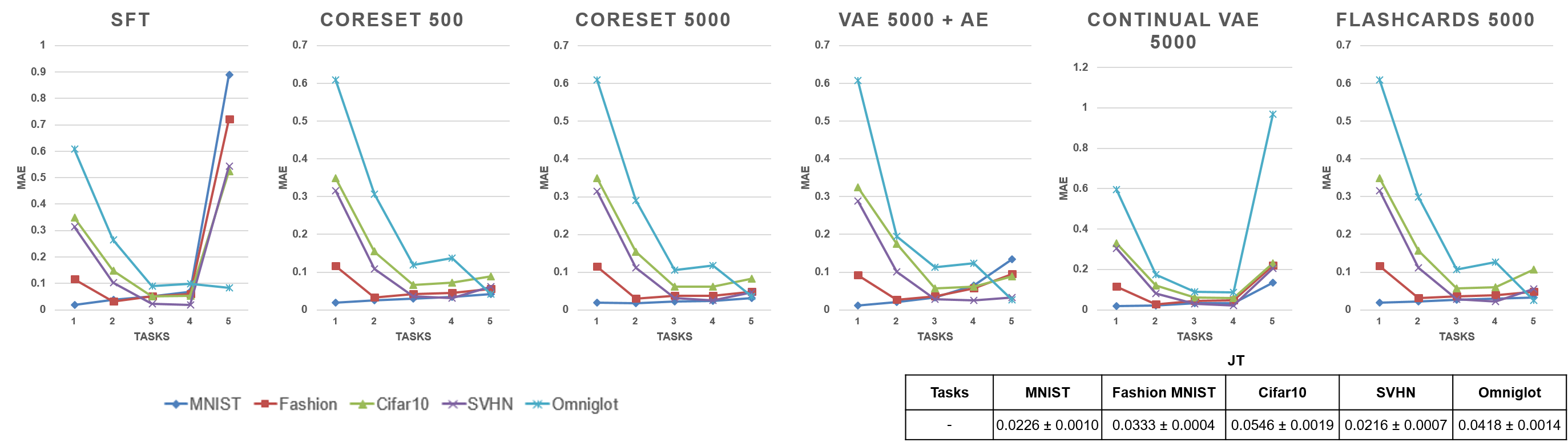
Figure 13: Continual Learning for Reconstruction. Individual graphs for different methods show the variation of test Mean Absolute Error (MAE) on current task dataset after observing the data for sequence of tasks. The table shows the test MAE for Joint Training (JT) method. The reported values in graph and table obtained over 5 experimental runs. The standard deviation is quite small and is not displayed on the graphs to avoid clutter.

Appendix I Sequence3 Continual Reconstruction

We also permuted the order by taking MNIST, Fashion MNIST and Cifar10, to further substantiate the effect of flashcards. Tables 5, 6, and 7 compare the mitigation of forgetting with flashcards.

Method	Task	MNIST	Fashion MNIST	Cifar10	Avg MAE
Joint Training	-	0.0141	0.0256	0.0629	0.0342
	1	0.0190	-	-	0.0190
Coreset Sampling 5000	2	0.0245	0.0388	-	0.0316
	3	0.0249	0.0395	0.0666	0.0436
	1	0.0190	-	-	0.0190
Lower Bound	2	0.0268	0.0268	-	0.0268
	3	0.0467	0.0469	0.0512	0.0482
	1	0.0190	-	-	0.0190
Flashcards 5000	2	0.0243	0.0310	-	0.0276
	3	0.0282	0.0366	0.0579	0.0409

Table 8: Sequence of 3 - Order: MNIST, Fashion MNIST, Cifar10 as 3 tasks. Tasks are added incrementally, and MAE is computed on each dataset after current task is completed.

Method	Task	Fashion MNIST	Cifar10	MNIST	Avg MAE
Joint Training	-	0.0141	0.0256	0.0629	0.0342
	1	0.0324	-	-	0.0324
Coreset Sampling 5000	2	0.0344	0.0589	-	0.0466
	3	0.0386	0.0661	0.0200	0.0415
	1	0.0324	-	-	0.0324
Lower Bound	2	0.0548	0.0564	-	0.0556
	3	0.0816	0.2996	0.0140	0.1317
	1	0.0324	-	-	0.0324
Flashcards 5000	2	0.0336	0.0520	-	0.0428
	3	0.0352	0.0637	0.0156	0.0381

Table 9: Sequence of 3 - Order: Fashion MNIST, Cifar10, MNIST as 3 tasks.

Method	Task	Cifar10	MNIST	Fashion MNIST	Avg MAE
Joint Training	-	0.0141	0.0256	0.0629	0.0342
	1	0.0515	-	-	0.0515
Coreset Sampling 5000	2	0.0639	0.0220	-	0.0429
	3	0.0654	0.0229	0.0336	0.0406
	1	0.0515	-	-	0.0515
Lower Bound	2	0.2602	0.0142	-	0.1372
	3	0.1233	0.0465	0.0371	0.0689
	1	0.0515	-	-	0.0515
Flashcards 5000	2	0.0625	0.0181	-	0.0403
	3	0.0664	0.0261	0.0308	0.0411

Table 10: Sequence of 3 - Order: Cifar10, MNIST, Fashion MNIST as 3 tasks.

Appendix J Sequence5 Continual Denoising - Adjusting the weight of noise factor

We increased the noise factor steadily to check for the value where reconstruction fails completely. Figure 14 shows the impact of reconstruction using flashcards for different noise level settings. As more noise is added, it becomes visually difficult to make out the underlying image. At factor of 0.3, it is observed the network is trying to retain partial outer boundary but has forgotten the denoising ability when seeing the last task Omniglot.

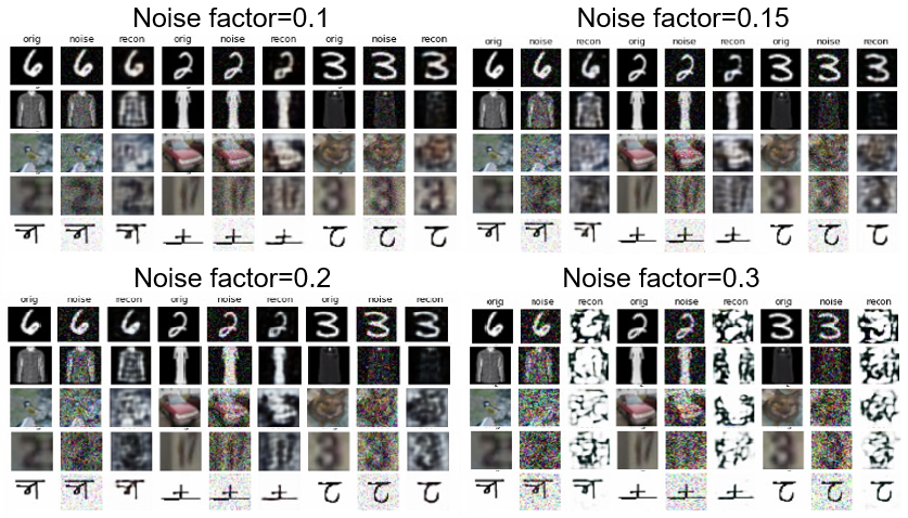
Figure 14: Continual Denoising scenario. Shown in figure is the effect of noise applied and the reconstruction of Sequence5 using flashcards.

Method/Sess	1	2	3	4	5
Cifar10
Naive	$67.90\pm 0.86$	$67.35\pm 0.81$	$67.66\pm 0.23$	$61.18\pm 0.96$	$63.05\pm 0.86$
Cumulative	$67.90\pm 0.86$	$69.74\pm 0.52$	$72.00\pm 0.28$	$72.85\pm 0.37$	$73.54\pm 0.22$
Coreset500	$67.90\pm 0.86$	$67.50\pm 0.24$	$68.29\pm 0.18$	$61.97\pm 0.82$	$63.85\pm 0.07$
Coreset5000	$67.90\pm 0.86$	$\textbf{68.47}\pm\textbf{0.51}$	$\textbf{68.38}\pm\textbf{0.79}$	$64.12\pm 0.46$	$65.18\pm 0.93$
Flashcards	$67.90\pm 0.86$	$68.05\pm 0.95$	$68.14\pm 1.27$	$\textbf{65.64}\pm\textbf{1.31}$	$\textbf{65.83}\pm\textbf{1.07}$
Cifar100
Naive	$37.67\pm 0.31$	$34.03\pm 0.53$	$35.10\pm 0.23$	$25.35\pm 0.69$	$28.74\pm 0.33$
Cumulative	$37.67\pm 0.31$	$40.63\pm 0.15$	$41.02\pm 0.18$	$41.24\pm 0.20$	$41.55\pm 0.11$
Coreset500	$37.67\pm 0.31$	$34.03\pm 0.51$	$34.95\pm 0.24$	$25.79\pm 1.55$	$29.09\pm 0.21$
Coreset5000	$37.67\pm 0.31$	$34.97\pm 0.08$	$35.02\pm 0.48$	$29.97\pm 0.07$	$30.63\pm 0.44$
Flashcards	$37.67\pm 0.31$	$\textbf{36.53}\pm\textbf{0.22}$	$\textbf{36.34}\pm\textbf{0.50}$	$\textbf{33.47}\pm\textbf{1.07}$	$\textbf{32.60}\pm\textbf{0.67}$

Table 11: ST-NIL Classification on Cifar10 and Cifar100 with mean and std.dev. over 5 runs.

Appendix K New Task Incremental Learning

This section provides architectural and training details for the Task-IL classification. Architecture of classifier is based on specifications from [van de Ven et al., 2020], and has five convolutional layers containing 16, 32, 64, 128 and 254 channels. Each layer used a 3×3 kernel, a padding of 1, and there was a stride of 1 in the first layer (i.e., no downsampling) and a stride of 2 in the other layers (i.e., image-size was halved in each of those layers). All convolutional layers used batch-norm followed by a ReLU non-linearity. The last conv layer is flattened to give 1024 dimensions, followed by a dense layer of 2000 activation followed by another dense layer of 128, forming the latent space. The output layer nodes were added based on the task and class information. Architecture for AE - encoder of classifier is shared with weights of trained classifier’s encoder and pre-initialized, but allowed to train further. Decoder is attached after latent space, and AE is trained by passing current task samples along with flashcards from AE upto current task.

Training details: For all tasks, mini-batch size of 256 and Adam optimizer with lr=0.0001 is used. Both models are trained for 5000 iterations. For 1st task, train classifier normally using crossentropy loss. Copy weights of classifier’s encoder to AE encoder. Train AE using mean square error (MSE) loss. From next task onwards, train classifier for new task along with constructed flashcards from AE of previous task. Output of flashcards is obtained by passing them to the classifier and obtaining soft labels, before the start of next task. Additionally, latent space activation can also be used to regularize the network further. After classifier is trained, copy weights of encoder to AE encoder and train AE with both current task and flashcards. Repeat process until end of all tasks.

Appendix L Single Task - New Instance Classification Forgetting Setting

We notice that the experimental setting mentioned in [Tao et al., 2020] does not reflect the forgetting scenario. Therefore, we introduce a more challenging setting across sessions: brightness_jitter = [0, -0.1, 0.1, -0.2, 0.2] and saturation_jitter = [0, -0.1, 0.1, -0.2, 0.2]. We employ the same learning parameters as described in their work, using ResNet18 as the classifier and optimizing using SGD with learning rates of 0.001 over 20 epochs. Results for Cifar10 and Cifar100 in Table 11 show replay using flashcards is at-par with episodic coreset replay.

References

- Aljundi et al. [2019] R. Aljundi, L. Caccia, E. Belilovsky, M. Caccia, M. Lin, and L. Charlin. Online continual learning with maximally interfered retrieval. Proceedings of the Advances in Neural Information Processing Systems 32, 2019.
- Bing [2020] Liu Bing. Learning on the job: Online lifelong and continual learning. In Proceedings of the AAAI, 2020.
- Castro et al. [2018] Francisco M Castro, Manuel J Marín-Jiménez, Nicolás Guil, Cordelia Schmid, and Karteek Alahari. End-to-end incremental learning. In Proceedings of the European conference on computer vision (ECCV), pages 233–248, 2018.
- Chaudhry et al. [2019] Arslan Chaudhry, Marc’Aurelio Ranzato, Marcus Rohrbach, and Mohamed Elhoseiny. Efficient lifelong learning with A-GEM. In ICLR, 2019.
- Devlin et al. [2019] J. Devlin, M. W. Chang, K. Lee, and K. Toutanova. BERT: Pre-training of deep bidirectional transformers for language understanding. In NAACL-HLT, 2019.
- Geirhos et al. [2019] Robert Geirhos, Patricia Rubisch, Claudio Michaelis, Matthias Bethge, Felix A. Wichmann, and Wieland Brendel. Imagenet-trained cnns are biased towards texture; increasing shape bias improves accuracy and robustness. In ICLR, 2019.
- Gou et al. [2020] Jianping Gou, Baosheng Yu, Stephen John Maybank, and Dacheng Tao. Knowledge distillation: A survey, 2020.
- Heusel et al. [2017] Martin Heusel, Hubert Ramsauer, Thomas Unterthiner, Bernhard Nessler, and Sepp Hochreiter. Gans trained by a two time-scale update rule converge to a local nash equilibrium. In Advances in neural information processing systems, pages 6626–6637, 2017.
- Hinton et al. [2015] Geoffrey Hinton, Oriol Vinyals, and Jeff Dean. Distilling the knowledge in a neural network. arXiv preprint arXiv:1503.02531, 2015.
- Kirkpatrick et al. [2017] J. Kirkpatrick, R. Pascanu, N. Rabinowitz, J. Veness, G. Desjardins, A. A. Rusu, K. Milan, J. Quan, T. Ramalho, and Grabska-Barwinska. Overcoming catastrophic forgetting in neural networks. Proceedings of the national academy of sciences, 114, 2017.
- Krizhevsky et al. [2012] A. Krizhevsky, I. Sutskever, and G. E. Hinton. Imagenet classification with deep convolutional neural networks. In Advances in neural information processing systems, 2012.
- Li and Hoiem [2018] Z. Li and D. Hoiem. Learning without forgetting. IEEE Transactions on Pattern Analysis and Machine Intelligence, 2018.
- Li et al. [2020] H. Li, W. dong, and B. G. Hu. Incremental concept learning via online generative memory recall. IEEE Transactions on Neural Networks and Learning Systems, 2020.
- Lomonaco and Maltoni [2017] Vincenzo Lomonaco and Davide Maltoni. Core50: a new dataset and benchmark for continuous object recognition. arXiv preprint arXiv:1705.03550, 2017.
- Lopez-Paz and Ranzato [2017] David Lopez-Paz and Marc' Aurelio Ranzato. Gradient episodic memory for continual learning. In Advances in Neural Information Processing Systems 30, 2017.
- Längkvist et al. [2014] M. Längkvist, L. Karlsson, and A. Loutfi. A review of unsupervised feature learning and deep learning for time-series modeling. Pattern Recognition Letters, 2014.
- Martin and Mahoney [2020] Charles H Martin and Michael W Mahoney. Heavy-tailed universality predicts trends in test accuracies for very large pre-trained deep neural networks. In Proceedings of the 2020 SIAM International Conference on Data Mining, 2020.
- Ostapenko et al. [2019] Oleksiy Ostapenko, Mihai Puscas, Tassilo Klein, Patrick Jahnichen, and Moin Nabi. Learning to remember: A synaptic plasticity driven framework for continual learning. In Proceedings of the CVPR, 2019.
- Parisi et al. [2019] German I. Parisi, Ronald Kemker, Jose L.Part, Christopher Kanan, and Stefan Wermter. Continual lifelong learning with neural networks: A review. Neural Networks, 2019.
- Robins [1995] Anthony Robins. Catastrophic forgetting, rehearsal and pseudorehearsal. Connection Science, 7(2):123–146, 1995.
- Rostami et al. [2020] M. Rostami, S. Kolouri, J. McClelland, and P. Pilly. Generative continual concept learning. Proceedings of the 34th AAAI, 2020.
- Tao et al. [2020] X. Tao, X. Hong, X. Chang, and Y. Gong. Bi-objective continual learning: Learning ’n’ew while consolidating ’known’. Proceedings of the 34th AAAI, 2020.
- Thrun [1996] Sebastian Thrun. Is learning the n-th thing any easier than learning the first? In Advances in neural information processing systems, pages 640–646, 1996.
- van de Ven et al. [2020] G. M. van de Ven, H. T. Siegelmann, and A. S. Tolias. Brain-inspired replay for continual learning with artificial neural networks. Nature Communications, 11, 2020.
- Zenke et al. [2017] Friedemann Zenke, Ben Poole, and Surya Ganguli. Continual learning through synaptic intelligence. In Proceedings of the 34th ICML - Volume 70, 2017.
- Zhuang et al. [2021] F. Zhuang, Z. Qi, K. Duan, D. Xi, Y. Zhu, H. Zhu, H. Xiong, and Q. He. A comprehensive survey on transfer learning. Proceedings of the IEEE, 109(1):43–76, 2021.