Blindfolded Attackers Still Threatening:
Strict Black-Box Adversarial Attacks on Graphs

Abstract

Adversarial attacks on graphs have attracted considerable research interests. Existing works assume the attacker is either (partly) aware of the victim model, or able to send queries to it. These assumptions are, however, unrealistic. To bridge the gap between theoretical graph attacks and real-world scenarios, in this work, we propose a novel and more realistic setting: strict black-box graph attack, in which the attacker has no knowledge about the victim model at all and is not allowed to send any queries. To design such an attack strategy, we first propose a generic graph filter to unify different families of graph-based models. The strength of attacks can then be quantified by the change in the graph filter before and after attack. By maximizing this change, we are able to find an effective attack strategy, regardless of the underlying model. To solve this optimization problem, we also propose a relaxation technique and approximation theories to reduce the difficulty as well as the computational expense. Experiments demonstrate that, even with no exposure to the model, the Macro-F1 drops 6.4% in node classification and 29.5% in graph classification, which is a significant result compared with existent works.

1 Introduction

Graph-based models, including graph neural networks (GNNs) Kipf and Welling (2017); Veličković et al. (2018) and various random walk-based models Lovász (1993); Perozzi et al. (2014), have achieved significant success in numerous domains like social network Pei et al. (2015), bioinformatics Gilmer et al. (2017), finance Paranjape et al. (2017), etc. However, these approaches have been shown to be vulnerable to adversarial examples Jin et al. (2020), namely those that are intentionally crafted to fool the models through slight, even human-imperceptible modifications to the input graph. Therefore, adversarial attack presents itself as a serious security challenge, and is of great importance to identify the weaknesses of graph-based models.

Information accessible	White-box	Gray-box	Restricted black-box	Black-box	Strict black-box
Model parameters	$\surd$	$\times$	$\times$	$\times$	$\times$
Labels	$\surd$	$\surd$	$\times$	$\times$	$\times$
Queries	$\surd$	$\times$	$\times$	$\surd$	$\times$
Model structure	$\surd$	$\bigcirc$	$\bigcirc$	$\times$	$\times$

Table 1: Different graph adversarial attacks, categorized by whether the attacker has full ($\surd$), limited ($\bigcirc$), or no ($\times$) access to the model.

Over recent years, extensive efforts have been devoted to studying adversarial attacks on graphs. According to the amount of knowledge accessible to the attacker, we summarize five categories of existing works in Table 1. As the first attempt, white-box attack assumes the attacker has full access to the victim model Wu et al. (2019); Xu et al. (2019a); Chen et al. (2018); Wang et al. (2018). Then gray-box attack is proposed, in which the attacker trains a surrogate model based on limited knowledge of the victim as well as task-specific labeled data Zügner et al. (2018); Zügner and Günnemann (2019). Whereas, most real-world networks are unlabeled and it is arduously expensive to obtain sufficient labels, which motivates the study of (restricted) black-box attacks. With no access to the correct labels, restricted black-box attack shows its success but still needs limited knowledge of the victim model Chang et al. (2020). Comparatively, the black-box model is not aware of the victim model, but has to query some or all examples to gather additional information Dai et al. (2018); Yu et al. (2020).

Despite these research efforts, there still exists a considerable gap between the existing graph attacks and the real-world scenarios. In practice, the attacker cannot fetch even the basic information about the victim model, for example, whether the model is GNN-based or random-walk-based. Moreover, it is also unrealistic to assume that the attacker can query the victim model in real-world applications. Such querying attempts will be inevitably noticed and blocked by the defenders. For example, a credit risk model built upon an online payment network is often hidden behind company API wrappers, and thus totally unavailable to the public.

In view of the above limits, we propose a new attack strategy, strict black-box graph attack (STACK), which has no knowledge of the victim model and no access to queries or labels at all. The design of such attack strategies is nontrivial due to the following challenges:

• Most existing graph attack strategies are model-specific, and are not extendable to the strict black-box setting. For example, the attack designed for the low-pass GNN filter Kipf and Welling (2017); Veličković et al. (2018) will inevitable perform badly on a GNN model that covers almost all frequency profiles because the attacker might target at some irrelevant bands of frequency. Thereby, the first challenge is to identify a common cornerstone for various types of graph-based models.

• Existing works always use model predictions or the feedback from surrogate models to quantify the effects of attacks. However, with no access to the queries and the correct labels, we can neither measure the quality of predictions, nor refer to a surrogate model. So the second challenge is how to effectively quantify the strength of graph attacks and efficiently compute them.

To handle the above challenges, we first propose a generic graph filter which formulates the key components of various graph models into a compact form. Then we are able to measure the strength of attacks by the change of the proposed graph filter before and after attack. An intuitive but provably effective attack strategy is to maximize this change within a fixed amount of perturbation on the original graph. To solve the optimization problem efficiently, we further relax the objective of this problem to a function of the eigenvalues, and then we show that the relaxed objective can be approximated efficiently via eigensolution approximation theories. Besides the reduction in computational complexity, this approximation technique also captures inter-dependency between edge flips, which is ignored in previous works Bojchevski and Günnemann (2019); Chang et al. (2020). In addition, a restart mechanism is applied to prevent accumulation of approximation errors without sacrificing the accuracy.

We summarize our major contributions as follows:

• We bring attention to a critical yet overlooked strict black-box setting in adversarial attacks on graphs.

• We propose a generic graph filter applicable to various graph models, and also develop an efficient attack strategy to select adversarial edges.

• Extensive experiments demonstrate that even when the attacker is unaware of the victim model, the Macro-F1 in node classification drops 6.4% and that of graph classification drops 29.5%, both of which are significant results compared with SOTA approaches.

The success of our STACK method breaks the illusion that perfect protection for the victim model could block all kinds of attacks: even when the attacker is totally unaware of the underlying model and the downstream task, it is still able to launch an effective attack.

2 Strict Black-box Attacks (STACK)

Let $G=(V,E)$ be an undirected and unweighted graph with the node set $V=\{v_{1},v_{2},...,v_{N}\}$ and the edge set $E\subseteq V\times V$. For simplicity we assume throughout the paper that the graph has no isolated nodes. The adjacency matrix $A$ of graph $G$ is an $N\times N$ symmetric matrix with elements $A_{ij}=1$ if $\{i,j\}\in E$ or $i=j$, and $A_{ij}=0$ otherwise. Note that we intentionally set the diagonal elements of $A$ to $1$. We also denote by $D$ the diagonal degree matrix with $D_{ii}=\sum_{i=1}^{N}A_{ij}$.

Suppose we have a graph model designed for certain downstream tasks (i.e., node classification, graph classification, etc.) The attacker is asked to modify the graph structure and/or node attributes within a fixed budget such that the performance of downstream task degrades as much as possible. Here we follow the assumption that the attacker will add or delete a limited number of edges from $G$, resulting in a perturbed graph $G^{\prime}=(V,E^{\prime})$. The setting is conventional in previous works Chen et al. (2018); Bojchevski and Günnemann (2019); Chang et al. (2020), and also practical in many scenarios like link spam farms Gyongyi and Garcia-Molina (2005), Sybil attacks Yu et al. (2006), etc.

Towards more practical scenarios, we assume the attacker can neither access any knowledge about the victim model nor query any examples. We call such attack as the strict black-box attack (STACK) on graphs. The attacker’s goal is to figure out which set of edges flips can fool various graph-based victim models when they are applied to different downstream tasks. The generality of the proposed attack model is guaranteed by a generic graph filter, which is introduced in §2.1, and in §2.2 we formulate an optimization problem for construction of such a model.

2.1 Generic Graph Filter

Without access to any information from victim models and queries, we need to take into account the common characteristics of various graph-based victim models when designing the adversarial attack. We therefore propose a generic graph filter $S$:

$$S=D^{-\alpha}AD^{-1+\alpha},$$ (1)

where $\alpha\in[0,1]$ is a given parameter to enlarge the filter family. Many common choices of graph filters can be considered as special cases of the generic graph filter $S$. For instance, when $\alpha=1/2$, the corresponding graph filter $S_{\mathrm{sym}}=D^{-1/2}AD^{-1/2}$ is symmetric, and used in numerous applications, including spectral graph theory Chung (1997) and the graph convolutional networks (GCNs) Kipf and Welling (2017); Veličković et al. (2018). Another common choice of $\alpha$ is $\alpha=1$, and the resulting graph filter $S_{\mathrm{rw}}=D^{-1}A$ is widely used in many applications related to random walks on graphs Chung (1997). It is well known that many graph properties (e.g., network connectivity, centrality) can also be expressed in terms of the proposed generic graph filter Lovász (1993). Furthermore, it is easy to see the relation between the graph Laplacian ($L=D-A$) and $S$, i.e., $S=I-D^{-\alpha}LD^{-1+\alpha}$, where the change in $S$ and the change in $D^{-\alpha}LD^{-1+\alpha}$ is exactly the same.

The proposed generic graph filters have many interesting properties. Firstly, its eigenvalues are invariant under isomorphic transformations, i.e., its intrinsic spectral properties (e.g., distances between vertices, graph cuts, the stationary distributions of a Markov chain Cohen et al. (2017)) are preserved regardless of the choice of $\alpha$. In addition, the eigenvalues of $S$ are bounded in $[-1,1]$. Hence, the generic graph filter of the original graph $G$ and that of the perturbed graph $G^{\prime}$ are more comparable from the perspective of graph isomorphism and spectral properties; see §3 for more details.

2.2 The Optimization Problem

With the mere observation of the input graph, our attacker aims to find the set of edge flips that would change the graph filter $S$ most. Considering the dependency structure between the nodes, one adversarial perturbation is easy to propagate to other neighbors via relational information. Therefore, the generic graph filter $S$ is used instead of the adjacency matrix $A$, because the impact of one edge flip on $S$ can properly depict such cascading effects on a graph. Similar ideas are conventional adopted by most graph learning models Chung (1997). To flip the most influential edges, we formulate our attack model as the following optimization problem:

$$\small\begin{array}[]{ll}\mbox{\normalsize maximize}&\mathcal{L}_{1}\left(A^{\prime}\right)=\left\|(S^{\prime})^{k}-S^{k}\right\|_{F}^{2}\\ \mbox{\normalsize subject to}&A^{\prime}_{ii}=1,\quad i=1,\ldots,N\\ &A^{\prime}_{ij}\in\{0,1\}\mbox{ for }i\neq j\\ &\|A^{\prime}-A\|_{0}\leq 2\delta,\end{array}$$ (2)

where the optimization variable is the $N\times N$ symmetric matrix $A^{\prime}$. The matrix power $S^{k}$ takes account of all the neighbors within $k$ hops (instead of those $k$-hop neighbors) because $A$ is defined to include self-loops. When targeting on localized kernels (e.g., GCN), we prefer $k=1$ or $2$, while a larger $k$ is recommended to capture higher-order structural patterns. The last inequality constraint shows the budget $\delta$ with $0<\delta\ll|E|$, which is consistent with most previous works Jin et al. (2020); Dai et al. (2018). The left part of Figure 1 gives an example of the proposed problem.

3 Methodology

Although the objective function $\mathcal{L}_{1}(A^{\prime})$ described in Problem (2) directly shows the difference between the original graph filter and the perturbed one, the evaluation of the objective function involves a costly eigenvalue decomposition, which in turn makes the whole problem expensive to solve. Therefore, in this section, we aim to find a sub-optimal solution to Problem (2), with a reasonable computation expense. This process is illustrated in Figure 1. In §3.1 we relax the original objective to a lower bound, which only involves the spectrum of graph filter; this corresponds to the upper-right part of Figure 1. Then, we give an approximate solution to compute the perturbed spectrum in §3.2, as shown in the lower-right corner of Figure 1. A detailed description of how to select adversarial edges is provided in §3.3 for solving the relaxed problem . Finally, in §3.4 we show that our model is flexibly extendable when more information is available.

3.1 A Viable Lower Bound for $\mathcal{L}_{1}$

To find such a relaxation of the objective function $\mathcal{L}_{1}(A^{\prime})$, we first observe that the eigenvalues of $S$ are independent of $\alpha$, due to the following lemma.

Lemma 1.

$\lambda$ is an eigenvalue of $S=D^{-\alpha}AD^{-1+\alpha}$ if and only if $(\lambda,u)$ solves the generalized eigenproblem $Au=\lambda Du$.

With Lemma 1, we specify $\alpha=1/2$ and are able to construct a convenient lower bound for $\mathcal{L}_{1}$, involving only the eigenvalues of $S^{\prime}$.

Theorem 1.

The function $\mathcal{L}_{1}(A^{\prime})$ is lower bounded by

$$\small\mathcal{L}_{1}(A^{\prime})\geq\left(\sqrt{\sum_{i=1}^{N}(\lambda^{\prime}_{i})^{2k}}-\sqrt{\sum_{i=1}^{N}\lambda_{i}^{2k}}\right)^{2}=\mathcal{L}_{2}(\lambda^{\prime}),$$ (3)

where $\lambda_{i}$ and $\lambda^{\prime}_{i}$ are the $i$-th generalized eigenvalue of $A$ and $A^{\prime}$, respectively, i.e., $Au_{i}=\lambda_{i}Du_{i}$ and $A^{\prime}u^{\prime}_{i}=\lambda^{\prime}_{i}D^{\prime}u^{\prime}_{i}$. We assume that both eigenvalue sequences are numbered in a non-increasing order.

Proofs and additional explanation of Lemma 1 and Theorem 1 can be found in §A.2.

Now the problem of maximizing $\mathcal{L}_{1}\left(A^{\prime}\right)$ can be properly relaxed to the problem of maximizing its lower bound $\mathcal{L}_{2}(\lambda^{\prime})$. Intuitively, $\mathcal{L}_{2}(\lambda^{\prime})$ is exactly describing the spectral change, which is a natural measure used in spectral graph theory Chung (1997). Additionally, Eq. (3) is also valid for any symmetric matrices $S$ and $S^{\prime}$; hence, the lower bound $\mathcal{L}_{2}(\lambda^{\prime})$ holds for different types of networks (e.g. weighted or unweighted) and different perturbation scenarios (e.g. adjusting edge weights).

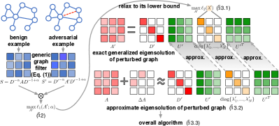
Figure 1: Overview of strict black-box adversarial attacks on graphs.

3.2 Approximating Perturbed Eigensolution

Although $\mathcal{L}_{2}(\lambda^{\prime})$ is a desirable lower bound for its flexibility, its computation remains a great challenge for two reasons.

First, the computation of $\mathcal{L}_{2}(\lambda^{\prime})$ relies on the eigenvalue decomposition of $A^{\prime}$, which costs $\mathcal{O}(N^{3})$ flops. What’s worse, this decomposition has to be re-evaluated again and again for every possible set of flipped edges, which turns out to be a computational bottleneck.

Moreover, the inter-dependency between adversarial edges should be taken into consideration. For example, the spectral change caused by flipping two edges $e_{1}$ and $e_{2}$ is not identical to the sum of the change caused by flipping $e_{1}$ and that caused by $e_{2}$. This difference has been ignored in most studies Bojchevski and Günnemann (2019); Chang et al. (2020) but might turn out to be critical in designing adversarial attacks. In this work, however, we fill this gap by describing such dependency as a combinatorial optimization problem, which is usually difficult to solve.

To resolve the above issues, we can apply the first-order eigenvalue perturbation theory Stewart and Sun (1990) to approximate $\mathcal{L}_{2}$. This approximation is accurate enough for our purpose because the perturbation on graphs is assumed to be extremely small, i.e., $\delta\ll|E|$. We start with the simplest case where only one edge is flipped Stewart and Sun (1990).

Theorem 2.

Let $\Delta A=A^{\prime}-A$ and $\Delta D=D^{\prime}-D$ be the perturbations of $A$ and $D$, respectively. Let $(\lambda_{k},u_{k})$ be the $k$-th generalized eigen-pair of $A$, i.e., $Au_{k}=\lambda_{k}Du_{k}$. Assume these eigenvectors are properly normalized so that ${u}^{\scriptscriptstyle T}_{j}Du_{i}=1$ if $i=j$ and $0$ otherwise. When only one edge $\{p,q\}$ is flipped, the perturbed $k$-th generalized eigen-pair can be approximated by

$$\lambda^{\prime}_{k}\approx\lambda_{k}+\Delta A_{pq}\big{(}2u_{kp}\cdot u_{kq}-\lambda_{k}(u_{kp}^{2}+u_{kq}^{2})\big{)}$$ (4)

$$u^{\prime}_{k}\approx\left(1-\frac{1}{2}\Delta A_{pq}\left(u_{kp}^{2}+u_{kq}^{2}\right)\right)u_{k}$$

$$+\sum_{i\neq k}\frac{\Delta A_{pq}\left(u_{ip}u_{kq}+u_{iq}u_{kp}-\lambda_{k}\left(u_{ip}u_{kp}+u_{iq}u_{kq}\right)\right)}{\lambda_{k}-\lambda_{i}}u_{i}$$ (5)

where $u_{kp}$ is the $p$-th entry of the vector $u_{k}$.

For one edge flip, the approximation of the eigenvalue $\lambda_{k}^{\prime}$ requires only $\mathcal{O}(1)$ flops to compute (cf. Eq. (4)). By ignoring dependency among adversarial edges, some previous works directly adopt Theorem 2 to approximate the spectrum change caused by each edge flip and choose the edges with the highest spectral impact to perturb Bojchevski and Günnemann (2019); Chang et al. (2020). To explore and utilize such dependency, we update the eigenvalues and eigenvectors after each edge flip, and then choose the subsequent edge flips based on the updated eigensolutions. However, the computational cost associated with re-evaluating the eigenvectors via Eq. (5) is still too high ($\mathcal{O}(N^{2})$ flops for each). What’s worse, Eq. (5) is valid only when all eigenvalues are distinct, which is not guaranteed in practice. Therefore, inspired by the power iteration, we propose the following theorem to approximate the perturbed eigenvectors.

Theorem 3.

Let $\Delta A=A^{\prime}-A$ and $\Delta D=D^{\prime}-D$ denote the perturbations of $A$ and $D$, respectively. Moreover, the number of non-zero entries of $\Delta A$ and $\Delta D$ are assumed to be much smaller than that of $A$ and $D$. Let $u_{k}$ be the $k$-th generalized eigenvector of $A$ with generalized eigenvalue $\lambda_{k}$. We first assume that the eigenvectors are properly normalized, such that $\|u_{k}\|_{2}=1$. The $k$-th generalized eigenvector $u^{\prime}_{k}$ can then be approximated by

$$\small u^{\prime}_{k}\approx\begin{cases}\displaystyle\mathbf{sign}(\lambda_{k})u_{k}+\frac{\Delta Cu_{k}}{|\lambda_{k}|},&\mbox{if }\lambda_{k}\neq 0\\ \displaystyle\frac{\Delta Cu_{k}}{\|\Delta Cu_{k}\|_{2}},&\mbox{if }\lambda_{k}=0.\end{cases}$$ (6)

where $\Delta C=(D+\Delta D)^{-1}(A+\Delta A)-D^{-1}A$. Specifically, when one edge $\{p,q\}$ is flipped, only the $p$-th and $q$-th elements of $u^{\prime}_{k}$ will be changed because only specific elements of $\Delta C$ are non-zero, i.e.,

$$\Delta C_{ij}=\begin{cases}A_{pj}^{\prime}/D_{pp}^{\prime}-A_{pj}/D_{pp},\quad&\mbox{if }j\in\mathcal{N}(p)\bigcup\{p,q\}\\ A_{qj}^{\prime}/D_{qq}^{\prime}-A_{qj}/D_{qq},&\mbox{if }j\in\mathcal{N}(q)\bigcup\{p,q\}\\ 0,&\mbox{otherwise,}\end{cases}$$

where $\mathcal{N}(p)$ indicates the set of neighbors of node $p$.

When only one edge is flipped, Eq. (6) suggests that the approximation of the perturbed eigenvector requires only $\mathcal{O}(N)$ flops for each, which is far more efficient than $\mathcal{O}(N^{2})$ utilizing Eq. (5). In addition, the evaluation of $u_{k}^{\prime}$ in Eq. (6) involves only the $k$-th eigenvalue $\lambda_{k}$, which removes the strict assumption regarding distinct eigenvalues.

3.3 Generating Adversarial Edges

Up to this point, we have aimed to flip $\delta$ edges so that $\mathcal{L}_{2}\left(\lambda^{\prime}\right)$ is maximized. Specifically, we first form a candidate set by randomly sampling several edge pairs, as in Bojchevski and Günnemann (2019). Our attack strategy involves three steps: (i) for each candidate, compute its impact $\mathcal{L}_{2}\left(\lambda^{\prime}\right)$ on the original graph, such that the eigenvalues can be approximated via Eq. (4); (ii) flip the candidate edge that scores highest on this metric; and (iii) recompute the eigenvalues (Eq. (4)) and eigenvectors (Eq. (6)) after each time an edge is flipped. These steps are repeated until $\delta$ edges have been flipped.

Restart mechanism. In the above strategy, the approximation of the statistic in step (iii) is efficient. However, it inevitably leads to serious error accumulation as more edges are flipped. A straightforward solution is to reset the aggregated error (i.e., recompute the exact eigensolutions) over periodic time. Thus, the question of when to restart should be answered carefully. Recall that in Theorem 2, the perturbed eigenvectors must be properly normalized so that ${u^{\prime}_{i}}^{\scriptscriptstyle T}D^{\prime}u^{\prime}_{i}=1$. Thus, we can perform an orthogonality check to verify whether the eigenvectors have been adequately approximated. Theoretically, if the perturbed eigenvectors are approximately accurate and normalized to ${u^{\prime}}^{\scriptscriptstyle T}D^{\prime}u^{\prime}$, then ${U^{\prime}}^{\scriptscriptstyle T}D^{\prime}U^{\prime}$ will be close to the identity matrix. Thus, we propose to use the average of the magnitudes of the non-zero off-diagonal terms of ${U^{\prime}}^{\scriptscriptstyle T}D^{\prime}U^{\prime}$ to infer the approximation error of the perturbed eigenvectors:

$$\small\epsilon=\frac{1}{N(N-1)}\sum_{i=1}^{N}\sum_{j\neq i}\left|S^{\prime}_{ij}\right|,$$ (7)

where $S^{\prime}={U^{\prime}}^{\scriptscriptstyle T}D^{\prime}U^{\prime}$. The smaller the value of $\epsilon$, the more accurate our approximation. Thereby, the approximation error $\epsilon$ is monitored in every iteration, and restart is performed when the error exceeds a threshold $\tau$. This restart technique ensures approximation accuracy and also reduces time complexity.

(Unattacked)

Rand.

Deg.

Betw.

Eigen.

DW

GF-Attack

GPGD

STACK-r-d

STACK-r

STACK

White-box

Cora-ML

GCN

0.82$\pm$0.8

1.97$\pm$0.8

1.12$\pm$0.4

1.22$\pm$0.4

0.28$\pm$0.3

0.85$\pm$0.3

1.34$\pm$0.5

4.22$\pm$0.6

4.03$\pm$0.6

5.02$\pm$0.4

5.27$\pm$0.3

11.36$\pm$0.5

Node2vec

0.79$\pm$0.8

6.37$\pm$1.8

5.40$\pm$1.6

3.33$\pm$1.0

2.84$\pm$1.0

3.25$\pm$1.3

5.76$\pm$1.5

5.33$\pm$1.8

5.82$\pm$1.7

6.92$\pm$1.0

8.29$\pm$1.0

(1.43$\pm$0.9)

Label Prop.

0.80$\pm$0.7

4.10$\pm$1.3

2.45$\pm$0.7

2.71$\pm$0.8

2.07$\pm$0.7

1.79$\pm$0.9

3.18$\pm$0.5

4.28$\pm$1.6

5.01$\pm$0.7

6.02$\pm$0.9

7.13$\pm$0.9

(1.05$\pm$1.0)

Citeseer

GCN

0.66$\pm$1.4

2.02$\pm$0.6

0.16$\pm$0.4

0.70$\pm$0.4

0.64$\pm$0.4

0.21$\pm$0.4

1.36$\pm$0.7

2.14$\pm$0.9

2.63$\pm$0.7

3.16$\pm$0.6

3.98$\pm$0.5

6.42$\pm$0.6

Node2vec

0.60$\pm$1.5

7.47$\pm$2.3

7.47$\pm$1.6

3.47$\pm$2.6

4.87$\pm$1.5

2.54$\pm$2.5

6.45$\pm$3.5

5.26$\pm$1.9

7.94$\pm$1.6

8.32$\pm$2.5

9.32$\pm$2.6

(0.12$\pm$1.0)

Label Prop.

0.64$\pm$0.8

6.70$\pm$2.0

3.47$\pm$0.8

6.00$\pm$1.7

5.36$\pm$0.6

3.00$\pm$0.8

6.99$\pm$1.0

5.14$\pm$1.9

6.66$\pm$1.3

7.79$\pm$0.9

8.16$\pm$0.9

(2.47$\pm$1.2)

Polblogs

GCN

0.96$\pm$0.7

1.91$\pm$1.5

0.03$\pm$0.2

1.72$\pm$0.6

0.67$\pm$0.5

0.01$\pm$0.4

1.15$\pm$0.4

2.35$\pm$1.8

3.06$\pm$1.2

4.30$\pm$1.2

5.32$\pm$1.1

3.88$\pm$1.1

Node2vec

0.95$\pm$0.3

3.01$\pm$0.7

0.04$\pm$0.6

3.07$\pm$0.6

1.84$\pm$0.3

0.18$\pm$0.4

1.00$\pm$0.5

2.49$\pm$0.6

2.57$\pm$0.9

2.74$\pm$0.5

3.79$\pm$0.5

(2.13$\pm$0.4)

Label Prop.

0.96$\pm$0.5

4.99$\pm$0.7

0.08$\pm$0.4

3.45$\pm$0.7

2.15$\pm$0.3

0.37$\pm$0.5

2.18$\pm$0.4

4.15$\pm$0.8

5.17$\pm$0.8

5.84$\pm$0.7

6.14$\pm$0.7

(2.28$\pm$0.5)

Table 2: We apply various node-level attacks to different graphs models and different datasets. We report the decrease in Macro-F1 score (in percent) on the test set after the attack is performed; the higher the better. We also report the Macro-F1 on the unattacked graph.

3.4 Extension to Different Knowledge Levels

Our proposed adversarial manipulation can also be easily extended to boost performance when additional knowledge (e.g., model structure, learned parameters) is available. One straightforward way of doing this would be adopt $\mathcal{L}_{2}\left(\lambda^{\prime}\right)$ as a regularization term. Thereby, complementary to other types of adversarial attacks (e.g., white- or gray-box), the proposed attack model facilitates rich discrimination on global changes in the spectrum.

As an example of the extension to gray-box attack, assume our goal is to attack a GNN designed for the semi-supervised node classification task. The attacker is able to alter both the graph structure and the node attributes, and its goal is to misclassify a specific node $v_{i}$. In this case, a surrogate model is built with all non-linear activation function removed Zügner et al. (2018); this is denoted as $Z=\mathrm{softmax}(S^{k}XW)$, where $X$ denotes the feature matrix and $W$ represents the learned parameters. Therefore, the combined attack model tries to solve the following optimization problem:

$$\mbox{maximize}\ \max_{c\neq c_{0}}(({S^{\prime}}^{k}X^{\prime}W)_{v_{i}c}-({S^{\prime}}^{k}XW)_{v_{i}c_{0}})+\gamma\mathcal{L}_{2}\left(\lambda^{\prime}\right)$$

where the variables are the graph structure $A^{\prime}$ and the feature matrix $X^{\prime}$, the scalar $c_{0}$ denotes the true label or the predicted label for $v_{i}$ based on the unperturbed graph $G$, while $c$ is the class of $v_{i}$ to which the surrogate model assigns. The constant $\gamma>0$ is a regularization parameter. Note that this case can also be considered as an extension to targeted attack.

4 Experiments

In this section, we evaluate the performance of the proposed method on both node classification and graph classification task. We also extend our model to white-box or targeted attacks, as explained in §3.4. In addition, we study the gap between the initial formulation (2) and the relaxed problem.

4.1 Experimental Setup

Datasets. For node-level attacks, we adopt three real-world networks for node classification task, Cora-ML, Citeseer, and Polblogs, and we follow the preprocessing in Dai et al. (2018). For graph-level attacks, we use two benchmark protein datasets Enzymes and Proteins for graph classification task. See details of each dataset in §A.5.

Baselines. We consider the following baselines.

• Rand.: this method randomly flips edges.

• Deg./Betw./Eigen. Bojchevski and Günnemann (2019): the flipped edges are selected in the decreasing order of the sum of the degrees, betweenness, or eigenvector centrality.

• DW: a black-box attack method designed for DeepWalk Bojchevski and Günnemann (2019).

• GF-Attack: targeted attack under the strict black-box setting Chang et al. (2020). We directly adopt it under our untargeted attack setting by selecting the edge flips on the decreasing order of the loss for SGC/GCN.

• GPGD (Graph Projected Gradient Descent): we apply the GPGD algorithm to solve Problem (2) Xu et al. (2019a).

• STACK-r-d: a variant of our method, where both the restart mechanism and the dependency among edge flips are not considered here. Specifically, the edge flips are selected on the decreasing order according to Eq. (4) in Theorem 2.

• STACK-r: another variant of our method, where the restart mechanism is not considered here.

Implementation details. For the node classification task, we choose GCN Kipf and Welling (2017), Node2vec Grover and Leskovec (2016) and Label Propagation Zhu and Ghahramani (2003) as the victim models. We set the training/validation/test split ratio as 0.1:0.1:0.8, and allow the attacker to modify 10% of the total edges. Comparatively, GIN Xu et al. (2019b) and Diffpool Ying et al. (2018) are used as victim models in the graph classification task due to their excellence. We follow the default setting in the above models, including the split ratio, and allow the attacker to modify 20% of the total edges.

Throughout the experiment, we follow the strict black-box setting. We set the spatial coefficient $k=1$ and the restart threshold $\tau=0.03$. The candidate set of adversarial edges is randomly sampled in every trial, and its size is set as 20K. As shown in Table 2, this randomness does not hurt the performance overall (Figure 4 in §A.7 for more details). The reported results are all averaged over 10 trials. More implementation details can be found in §A.6.

4.2 Experimental Results

Node classification task. Table 2 reports the decrease in Macro-F1 score (in percent) in node classification for all the three datasets and three victim models. We can see that our method performs the best across all datasets. First, heuristics (Rand., Deg., Betw., and Eigen.) fail to find the most influential edges in strict black-box setting. Previous works (DW and GF-Attack) do not perform well either, mainly due to the blindness to additional information (i.e., model type). The limit of GPGD is probably attributed to its relaxation from the binary graph topology to the convex hull. The ablation study on Ours-r-d and Ours-r further highlights the significance of the edge dependencies and the restart mechanism. In addition, the last column in Table 2 shows the results of white-box attacks which applies GPGD for GCN Xu et al. (2019a). The original paper presents great success when using GCN as the victim model. But our experiments show the failure of its intuitive extension to node-embedding models (e.g., Node2vec) and diffusion models (e.g., Label Propagation).

		Rand.	Deg.	Betw.	Eigen.	DW	GF-Attack	GPGD	STACK-r-d	STACK-r	STACK
Proteins	GIN	9.05	9.31	12.50	8.00	13.44	10.82	9.49	11.48	12.81	13.53
	Diffpool	24.13	11.27	9.87	11.03	12.71	21.99	14.53	23.49	24.87	24.88
Enzymes	GIN	32.76	34.38	34.75	40.25	38.76	35.48	35.63	36.00	37.46	39.90
	Diffpool	38.09	17.48	9.51	17.74	13.55	37.19	20.32	38.18	40.18	39.62

Table 3: Graph-level attacks against GIN and Diffpool. We report the decrease in the
Macro-F1 score (in percent) on test set. Higher numbers indicate better performance.

	Nettack	STACK-ext
Cora-ML	55.70 (0.53)	59.75 (0.57)
Citeseer	63.41 (0.60)	65.58 (0.63)
Polblogs	5.16 (0.23)	5.40 (0.23)

Table 4: Extension to Nettack. We report the average decrease in prediction confidence (in percent) of true labels and the misclassification rate in parentheses.

Graph classification task. Table 4 reports the results in graph classification. Especially, our method is 2.65% on average better than other methods in terms of Macro-F1. Interestingly, STACK-r (without restart) sometimes performs well, indicating that we can apply a version with lower complexity in practice yet not sacrificing much accuracy.

Extension when additional knowledge is available. Here we explore whether our attack can be successfully extended as the example in §3.4. Specifically, we focus on the Nettack model Zügner et al. (2018) and follow their targeted attack settings. We randomly select 30 correctly-classified nodes from the test set and mount targeted attacks on these nodes. From Table 4, we see that the naive extension of our method can further drop 4.84% in terms of prediction confidence and increase 4.18% in terms of misclassification rate on average.

Approximation quality. From the original objective function $\mathcal{L}_{1}$ to our final model, we have made one relaxation and one approximation; both steps would accumulate errors in evaluating the original objective. One thing worth noting is that the estimation error caused by sampling can be ignored here, as demonstrated in Bojchevski and Günnemann (2019).

To evaluate the effectiveness of eigen-approximation, we first generate the following random graphs with 1K nodes: Erdős–Rényi Bollobás (2013), Barabási–Albert Albert and Barabási (2002), Watts–Strogatz Watts and Strogatz (1998), and Triad Formation Holme and Kim (2002). Then we flip 10 edges in every synthetic graph and compare the true eigenvalues with approximated ones. Figure 2 presents the average results of 100 repeated experiments, where x-axis denotes the approximated value, and y-axis indicates the actual value. The approximate linearity of the plotted red points suggests the effectiveness of our eigensolution approximation with restart algorithm (§3.3). As an ablation study, results generated by our algorithm without the restart step (blue points) shows a tendency of overestimating the change in eigenvalues before and after attacks.

Furthermore, we study the quality of relaxation and approximation by examining the gap between $\mathcal{L}_{1}$ and $\mathcal{L}_{2}$. We compute their Pearson and Spearman correlation coefficients on three real-world datasets in Table 5. Results are all close to 1, which indicates a linear correlation between the original objective $\mathcal{L}_{1}$ and the approximation of $\mathcal{L}_{2}$.

In addition to experiments mentioned in this section, we discuss additional experimental results in §A.7.

	Cora-ML	Citeseer	Polblogs
Pearson	$0.89$	$0.91$	$0.85$
Spearman	$0.91$	$0.93$	$0.93$

Table 5: The Pearson and Spearman correlation coefficients between $\mathcal{L}_{1}$ and approximated $\mathcal{L}_{2}$.

5 Related Work

We classify the category of graph adversarial attacks into white-box, gray-box, restricted black-box, black-box and strict black-box settings (cf. Table 1). Specifically, the training of most white-box attacks involve a gradient w.r.t the input of the model Wu et al. (2019); Xu et al. (2019a); Chen et al. (2018); Wang et al. (2018). For gray-box attacks, one common method is to train substitute models as surrogates to estimate the information of the victim models Zügner et al. (2018); Zügner and Günnemann (2019); Bojchevski and Günnemann (2019). Under restricted black-box attacks, Chang et al. (2020) assume the family of graph-based models (i.e., GNN-based or sampling-based) is known and design a graph signal processing-based attack method. For black-box attacks, Dai et al. (2018) employ a reinforcement learning-based method and a genetic algorithm to learn from queries of some or all of the examples. More practically, the strict black-box attacks assume the attacker has totally no knowledge of the victim model and queries. Besides, another line of work Ma et al. (2020), not part of the four categories, assume the victim model is GNN-based but the training input is partly available, which is anther view of practical merit.

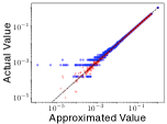
(a) Erdős–Rényi

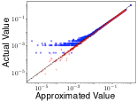
(b) Barabási–Albert

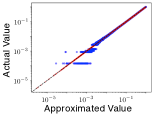
(c) Watts–Strogatz

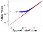
(d) Traid Formation

Figure 2: The true eigenvalues (y-axis) are plotted against the approximations (x-axis) in log scale. We present our approximations with (red plus) and without (blue circle) the restart step.

6 Conclusion

In this paper, we describe a strict black-box setting for adversarial attacks on graphs: the attacker not only has zero knowledge about the victim model, but is unable to send any queries as well. To handle this challenging but more realistic setting, a generic graph filter is proposed to unify different families of graph models; and its change is used to quantify the strength of attacks. By maximizing this change, we are always able to find an effective attack strategy. For efficient solution to the problem, we also propose a relaxation technique and an approximation algorithm. Extensive experiments show that the proposed attack strategy substantially outperforms other existing methods. For future work, we aim to extend STACK to be feasible on node- and attribute-level perturbations.

Appendix A Appendix

A.1 Notations

The main notations can be found in the Table 6.

Notation	Description
$G,A,S,E$	The original graph, the adjacency matrix, the generic graph filter and the edge set of $G$
$G^{\prime},A^{\prime},S^{\prime},E^{\prime}$	The perturbed graph, the adjacency matrix, the generic graph filter and the edge set of $G^{\prime}$
$u,u^{\prime}$	The generalized eigenvectors of $A$ and $A^{\prime}$
$\lambda,\lambda^{\prime}$	The generalized eigenvalues of $A$ and $A^{\prime}$
$\lambda(A),\lambda(A^{\prime})$	The eigenvalues of $A$ and $A^{\prime}$
$\lambda(S),\lambda(S^{\prime})$	The eigenvalues of $S$ and $S^{\prime}$
$\alpha$	The normalization parameter of the generic graph filter $S$
$\delta$	The perturbation budget
$k$	The spatial coefficient
$\tau$	The restart threshold
$r$	The number of restart
$\epsilon$	The approximation error of the perturbed eigenvectors

Table 6: Definition of major symbols.

A.2 Proofs and Derivations

Proof of Lemma 1.

$Au=\lambda Du$ implies

$$(D^{-\alpha}AD^{-1+\alpha})(D^{1-\alpha}u)=\lambda(D^{1-\alpha}u)$$

for any real symmetric $A$ and any positive definite $D$, which completes the proof. ∎

Proof of Theorem 1.

According to the triangle inequality, $\mathcal{L}_{1}(A^{\prime})$ is lower bounded by

$$\|(S^{\prime})^{k}-S^{k}\|_{F}^{2} \geq(\|(S^{\prime})^{k}\|_{F}-\|S^{k}\|_{F})^{2}$$

$$=\left(\sqrt{\sum_{i=1}^{n}\lambda_{i}(S^{\prime})^{2k}}-\sqrt{\sum_{i=1}^{n}\lambda_{i}\left(S\right)^{2k}}\right)^{2}$$

$$=\left(\sqrt{\sum_{i=1}^{N}(\lambda^{\prime}_{i})^{2k}}-\sqrt{\sum_{i=1}^{N}\lambda_{i}^{2k}}\right)^{2},$$

where the last step follows from Lemma 1.

By applying the Weyl’s inequalities (cf. Theorem 6 in § A.3) Horn and Johnson (2008) twice, and according to $(d^{\prime}_{1})^{-\alpha}\geq(d^{\prime}_{2})^{-\alpha}\geq\cdots\geq(d^{\prime}_{N})^{-\alpha}$ and $(d^{\prime}_{1})^{-1+\alpha}\geq(d^{\prime}_{2})^{-1+\alpha}\geq\cdots\geq(d^{\prime}_{N})^{-1+\alpha}$ because $\alpha\in[0,1]$, we have

$$\lambda_{i}\left(S^{\prime}\right) =\lambda_{i}\left({D^{\prime}}^{-\alpha}A^{\prime}{D^{\prime}}^{-1+\alpha}\right)$$

$$\leq\lambda_{1}\left({D^{\prime}}^{-\alpha}\right)\lambda_{i}\left(A^{\prime}{D^{\prime}}^{-1+\alpha}\right)$$

$$\leq\lambda_{1}\left({D^{\prime}}^{-\alpha}\right)\lambda_{i}\left(A^{\prime}\right)\lambda_{1}\left({D^{\prime}}^{-1+\alpha}\right)$$

$$={d^{\prime}_{1}}^{-\alpha}\lambda_{i}\left(A^{\prime}\right){d^{\prime}_{1}}^{-1+\alpha}$$

$$=\frac{1}{d_{\min}^{\prime}}\lambda_{i}\left(A^{\prime}\right),$$

where $\lambda_{1}$ is the largest eigenvalue and $d^{\prime}_{1}=d^{\prime}_{\min}$ is the smallest degree in $G^{\prime}$. ∎

Proof of Theorem 3..

According to one iteration of power iteration, when $\lambda_{k}\neq 0$,

$$u^{\prime}_{k} \approx\frac{(D+\Delta D)^{-1}(A+\Delta A)u_{k}}{\left\|(D+\Delta D)^{-1}(A+\Delta A)u_{k}\right\|_{2}}$$

$$=\frac{(D^{-1}A+\Delta C)u_{k}}{\left\|(D^{-1}A+\Delta C)u_{k}\right\|_{2}}$$

$$=\frac{\lambda_{k}u_{k}+\Delta Cu_{k}}{\left\|\lambda_{k}u_{k}+\Delta Cu_{k}\right\|_{2}}$$ (8)

$$=\frac{\lambda_{k}u_{k}+\Delta Cu_{k}}{\sqrt{\lambda_{k}^{2}{u_{k}}^{\scriptscriptstyle T}u_{k}+2\lambda_{k}{u_{k}}^{\scriptscriptstyle T}\Delta Cu_{k}+{u_{k}}^{\scriptscriptstyle T}\Delta{C}^{\scriptscriptstyle T}\Delta Cu_{k}}}$$

$$\approx\frac{\lambda_{k}u_{k}+\Delta Cu_{k}}{|\lambda_{k}|}=\mathbf{sign}(\lambda_{k})u_{k}+\frac{\Delta Cu_{k}}{|\lambda_{k}|}.$$

When $\lambda_{k}=0$, we can derive from (8) that $u_{k}^{\prime}\approx(\Delta Cu_{k})/(\|\Delta Cu_{k}\|_{2})$. ∎

A.3 Additional Theorems

Theorem 4.

(Eigenvalue perturbation theory Stewart and Sun (1990)). Let $\Delta A=A^{\prime}-A$ and $\Delta D=D^{\prime}-D$ be the perturbations of $A$ and $D$, respectively. Moreover, the number of non-zero entries of $\Delta A$ and $\Delta D$ are assumed to be much smaller than that of $A$ and $D$. Let $(\lambda_{k},u_{k})$ be the $k$-th pair of generalized eigenvalues and eigenvectors of $A$, i.e., $Au_{k}=\lambda_{k}Du_{k}$. We assume that these eigenvectors are properly normalized such that they satisfy ${u_{j}}^{\scriptscriptstyle T}Du_{i}=1$ if $i=j$ and $0$ otherwise. Thus, the $k$-th generalized eigenvalue $\lambda^{\prime}_{k}=\lambda_{k}+\Delta\lambda_{k}$ can be approximated by

$$\lambda^{\prime}_{k}\approx\lambda_{k}+{u_{k}}^{\scriptscriptstyle T}(\Delta A-\lambda_{k}\Delta D)u_{k}.$$

Moreover, when the eigenvalues are distinct, the $k$-th generalized eigenvector $u^{\prime}_{k}$ of $A^{\prime}$ can be approximated by

$$u^{\prime}_{k}\approx\left(1-\frac{1}{2}{u_{k}}^{\scriptscriptstyle T}\Delta Du_{k}\right)u_{k}+\sum_{i\neq k}\frac{{u_{i}}^{\scriptscriptstyle T}(\Delta A-\lambda_{k}\Delta D)u_{k}}{\lambda_{k}-\lambda_{i}}u_{i}.$$

Theorem 5.

(Bound of eigenvalues of $S^{\prime}$). The $i$-th generalized eigenvalue of $A^{\prime}$ (i.e., the $i$-th eigenvalue of $S^{\prime}$) is upper bounded by

$$\small\lambda^{\prime}_{i}=\lambda_{i}(S^{\prime})\leq\frac{1}{d_{\min}^{\prime}}\cdot\lambda_{i}(A^{\prime}),$$ (9)

where $d^{\prime}_{\min}$ is the smallest degree in $G^{\prime}$, $\lambda_{i}(S^{\prime})$ and $\lambda_{i}(A^{\prime})$ are the $i$-th eigenvalue of $S^{\prime}$ and $A^{\prime}$, respectively. This suggests that the eigenvalues of $S^{\prime}$ are always bounded by the eigenvalues of $A^{\prime}$.

Theorem 6.

(Weyl’s inequality for singular values Horn and Johnson (2008)). Let two symmetric matrices $P,Q\in\mathbb{R}^{N\times N}$. Then, for the decreasingly ordered singular values $\sigma$ of $P$, $Q$ and $PQ$, we have $\sigma_{i+j-1}(PQ)\leq\sigma_{i}(Q)\times\sigma_{j}(Q)$ for any $1\leq i,j\leq N$ and $i+j\leq N+1$.

A.4 Algorithm

Our detailed attack strategy in given in Algorithm 1.

Algorithm 1 Overall attack strategy via eigensolution approximation with restart.

Input: Graph $G=(A)$, perturbation budget $\delta$, restart threshold $\tau$.

Output: Modified Graph $G^{\prime}\leftarrow(A^{\prime})$.

1:  $A^{\prime}\leftarrow A$, $D^{\prime}\leftarrow D$;

2:  Solve the exact eigensolutions: $A^{\prime}u^{\prime}=\lambda^{\prime}D^{\prime}u^{\prime}$;

3:  $\text{Cand}\leftarrow\operatorname{candidate}(A^{\prime})$;

4:  while $\left\|A^{\prime}-A\right\|_{0}\leq 2\delta$ do

5:     $e^{\prime}\leftarrow\underset{e\in\text{Cand}}{\operatorname{argmax}}\ \mathcal{L}_{2}(e)$, which is approximated via Eq. 4;

6:     $A^{\prime},D^{\prime}\leftarrow$ insert or remove $e^{\prime}$ to/from $A^{\prime}$;

7:     Approximately update eigenvalue $\lambda^{\prime}$ via Eq. 4 and update eigenvector $u^{\prime}$ via Eq. 6;

8:     if $u^{\prime}!=\textbf{0}$ then

9:        Normalize the perturbed eigenvector $u^{\prime}$ s.t. ${u^{\prime}_{j}}^{\scriptscriptstyle T}Du^{\prime}_{i}=1$ if $i=j$;

10:        Compute $\epsilon$ via Eq. 7;

11:        if $\epsilon>\tau$ then

12:           Recompute the exact eigensolutions;

13:        end if

14:     else

15:        Recompute the exact eigensolutions;

16:     end if

17:     $\text{Cand}\leftarrow$ remove $e^{\prime}$;

18:  end while

19:  $G^{\prime}\leftarrow(A^{\prime})$.

A.5 Dataset Details

Synthetic datasets. We use four synthetic random graphs to evaluate the approximation quality. All synthetic graphs have 1000 nodes and parameters are chosen so that the average degree is approximately 10. Specifically, for the Erdős–Rényi graph, we set the probability for edge creation as 0.01. For the Barabási–Albert graph, we set the number of edges attached from a new node to existing nodes as 5. When generating the Watts–Strogatz graph, each node is connected to its 10 nearest neighbors in a ring topology, and the probability of rewiring each edge is 0.1. When generating growing graphs with the power-law degree distribution  Holme and Kim (2002), the number of random edges to add for each new node is 5, and the probability of adding a triangle after adding a random edge is 0.1.

Real-world datasets. We use three social network datasets: Cora-ML, Citeseer and Polblogs. The former two are citation networks mainly containing machine learning papers. Here, nodes are documents, while edges are the citation links between two documents. Each node has a human-annotated topic as the class label as well as a feature vector. The feature vector is a sparse bag-of-words representation of the document. All nodes are labeled to enable differentiation between their topic categories. Polblogs is a network of weblogs on the subject of US politics. Links between blogs are extracted from crawls of the blog’s homepage. The blogs are labelled to identify their political persuasion (liberal or conservative). Detailed statistics of the social network datasets are listed in Table 7.

We also use two protein graph datasets: Proteins and Enzymes. Proteins is a dataset in which nodes represent secondary structure elements (SSEs) and two nodes are connected by an edge if they are neighbors in either the amino-acid sequence or 3D space. The label indicates whether or not a protein is a non-enzyme. Moreover, Enzymes is a dataset of protein tertiary structures. The task is to correctly assign each enzyme to one of the six EC top-level classes. More detailed statistics of the protein graph datasets are listed in Table 8.

dataset	Cora-ML	Citeseer	Polblogs
type	citation network	citation network	web network
# vertices	2,810	2,110	1,222
# edges	7,981	3,757	16,714
# classes	7	6	2
# features	1,433	3,703	0

Table 7: Data statistics of social datasets.

dataset	Proteins	Enzymes
type	protein network	protein network
# graphs	1,113	600
# classes	2	6
# features	3	3
avg # nodes	39.06	32.63
avg # edges	72.82	62.14

Table 8: Data statistics of protein datasets.

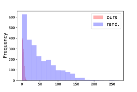
(a) Degree centrality

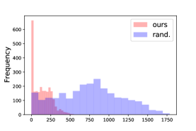
(b) Betweenness centrality

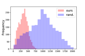
(c) Eigenvector centrality

Figure 3: The comparison of the centrality distributions for our selected adversarial edges and those of the randomly selected edges on Polblogs dataset.

A.6 Implementation Details

Here, we provide additional implementation details of our experiments in § 4.

For GCN, GIN and Diffpool, we use PyTorch Geometric  for implementation. We set the learning rate as 0.01 and adopt Adam as our optimizer. For Node2vec, we use its default hyper-parameter setting Grover and Leskovec (2016), but set the embedding dimension to 64 and use the implementation by CogDL . A logistic regression classifier is then used for classification given the embedding. For Label Propagation, we use an implementation that is adapted to graph-structured data .

For all victim models, we tune the number of epochs based on convergence performance. When performing GCN on Cora-ML, Citeseer and Polblogs, the number of epochs is set to 100. When performing GIN or Diffpool on Enzymes, we set the number of epochs to 20, while when performing GIN on Proteins, the number of epochs is set to 10. Finally, when performing Diffpool on Proteins, the number of epochs is set to 2. We conduct all experiments on a single machine of Linux system with an Intel Xeon E5 (252GB memory) and a NVIDIA TITAN GPU (12GB memory).

When implementing baselines, we directly apply the default hyperparameters of DW Bojchevski and Günnemann (2019), another black-box attack Chang et al. (2020) and Nettack Zügner et al. (2018). For GPGD Xu et al. (2019a) adopting $\mathcal{L}_{1}\left(A^{\prime}\right)$ as the objective, we train 500 epochs with a decaying learning rate as $\text{lr}=\text{lr\_init}(1/(1+i*\text{decay\_rate}))$ where lr_init is the initial learning rate, decay_rate is the decaying rate and $i$ is the current number of iterations. We set the initial learning rate as 2e-4 with a decaying rate 0.2 on Cora-ML, set the initial learning rate 1e-3 as with a decaying rate 0.2 on Citeseer, Polblogs, and set the initial learning rate 1e-2 as with a decaying rate 0.2 on Proteins and Enzymes. When applying GPGD for the white-box setting, we set the learning rate as 10 and run 700 epochs.

A.7 Additional Experimental Results

Node-level attack with increasing perturbation rate. Table 9 further shows that under increasing perturbation rates (5/10/15%), our node-level attacker can do more damage to GCN while still achieves the best performance. Note that when the perturbation rate is not very high, our solution without restart is already good enough to mount attacks.

	5%	10%	15%		5%	10%	15%
Rand.	0.75	1.97	2.41	GPGD	3.94	4.22	5.03
Deg.	0.59	1.12	1.34	GF-Attack	1.10	1.34	2.11
Betw.	0.63	1.22	1.45	STACK-r-d	3.90	4.03	5.11
Eigen.	0.30	0.28	1.12	STACK-r	4.43	5.02	5.77
DW	0.34	0.85	1.23	STACK	4.30	5.27	6.40

Table 9: Decrease in Macro-F1 score with different perturbation rates when attacking GCN on Cora-ML.

Attacks on Defensive models. We further validate the effectiveness of our attacks against three defensive models: EdgeDrop Dai et al. (2018), Jaccard Wu et al. (2019) and SVD Entezari et al. (2020). We utilize GCN as the backbone classifier and test on node classification task. We compare our method with the strongest competitor GPGD. The experimental settings are the same as those used in node-level attack. The results in Table 10 demonstrate that our method outperforms GPGD in terms of its ability to attack the defensive models. We can see that EdgeDrop cannot effectively defend against our attack, while the two pre-processing defense approaches (Jaccard and SVD) can defend against our attack to a certain extent.

	w/o defense	EdgeDrop	Jaccard	SVD
GPGD	4.22	6.04	3.94	3.47
STACK	5.27	7.11	4.71	4.02

Table 10: Attack against defensive models on Cora-ML. The decrease in Macro-F1 score is reported here.

		$\mathcal{L}^{*}_{1}$	$\mathcal{L}^{*}_{2}$	STACK
Cora-ML	GCN	1.92	1.72	5.27
	Node2vec	8.05	8.14	8.29
	Label Prop.	5.32	5.37	7.13
Citeseer	GCN	1.65	2.27	3.98
	Node2vec	8.64	9.05	9.32
	Label Prop.	7.09	5.41	8.16
Polblogs	GCN	2.65	2.92	5.32
	Node2vec	3.68	3.43	3.79
	Label Prop.	4.80	4.20	6.14

Table 11: The experimental results of other objective functions of node-level attacks against three types of victim models. We report the decrease in Macro-F1 score (in percent) on the test set after the attack.

(Unattacked)

Rand.

Deg.

Betw.

Eigen.

DW

GF-Attack

GPGD

STACK-r-d

STACK-r

STACK

White-box

Cora-ML

GCN

F1

0.82$\pm$0.8

1.97$\pm$0.8

1.12$\pm$0.4

1.22$\pm$0.4

0.28$\pm$0.3

0.85$\pm$0.3

1.34$\pm$0.5

4.22$\pm$0.6

4.03$\pm$0.6

5.02$\pm$0.4

5.27$\pm$0.3

11.36$\pm$0.5

Prec.

0.81$\pm$0.9

0.55$\pm$0.5

0.20$\pm$0.4

0.11$\pm$0.3

0.18$\pm$0.3

0.32$\pm$0.2

0.41$\pm$0.5

1.69$\pm$0.6

1.44$\pm$0.6

3.02$\pm$0.4

3.43$\pm$0.3

6.58$\pm$0.6

Recall

0.82$\pm$1.1

1.15$\pm$0.9

0.94$\pm$0.4

1.23$\pm$0.6

0.49$\pm$0.4

0.87$\pm$0.4

1.50$\pm$0.6

2.51$\pm$0.6

2.10$\pm$0.6

3.84$\pm$0.4

4.05$\pm$0.4

6.87$\pm$0.4

2-13

Node2vec

F1

0.79$\pm$0.8

6.37$\pm$1.8

5.40$\pm$1.6

3.33$\pm$1.0

2.84$\pm$1.0

3.25$\pm$1.3

5.76$\pm$1.5

5.33$\pm$1.8

5.82$\pm$1.7

6.92$\pm$1.0

8.29$\pm$1.0

(1.43$\pm$0.9)

Prec.

0.78$\pm$0.7

6.06$\pm$1.8

3.04$\pm$1.7

3.64$\pm$0.9

2.15$\pm$1.1

2.96$\pm$1.3

5.03$\pm$1.4

4.96$\pm$1.7

5.21$\pm$1.6

5.95$\pm$1.0

8.04$\pm$1.0

(1.39$\pm$1.0)

Recall

0.78$\pm$0.9

6.69$\pm$2.0

3.76$\pm$1.5

4.92$\pm$1.3

3.01$\pm$1.0

3.57$\pm$1.4

5.22$\pm$1.6

5.10$\pm$1.8

5.30$\pm$1.7

6.32$\pm$1.0

8.54$\pm$0.9

(1.52$\pm$1.1)

2-13

Label Prop.

F1

0.80$\pm$0.7

4.10$\pm$1.3

2.45$\pm$0.7

2.71$\pm$0.8

2.07$\pm$0.7

1.79$\pm$0.9

3.18$\pm$0.5

4.28$\pm$1.6

5.01$\pm$0.7

6.02$\pm$0.9

7.13$\pm$0.9

(1.05$\pm$1.0)

Prec.

0.81$\pm$0.8

2.98$\pm$1.3

1.10$\pm$0.6

1.20$\pm$0.4

1.46$\pm$0.7

1.05$\pm$0.8

2.74$\pm$0.4

3.05$\pm$1.0

4.10$\pm$0.6

4.62$\pm$0.8

4.98$\pm$1.0

(0.09$\pm$0.8)

Recall

0.80$\pm$1.0

4.95$\pm$1.2

3.61$\pm$0.9

4.32$\pm$1.0

2.64$\pm$0.9

2.54$\pm$1.2

4.71$\pm$0.6

5.03$\pm$1.9

5.15$\pm$0.7

7.92$\pm$1.0

7.99$\pm$1.0

(1.51$\pm$1.0)

Citeseer

GCN

F1

0.66$\pm$1.4

2.02$\pm$0.6

0.16$\pm$0.4

0.70$\pm$0.4

0.64$\pm$0.4

0.21$\pm$0.4

1.36$\pm$0.7

2.14$\pm$0.9

2.63$\pm$0.7

3.16$\pm$0.6

3.98$\pm$0.5

6.42$\pm$0.6

Prec.

0.64$\pm$1.6

1.15$\pm$0.7

0.10$\pm$0.5

0.33$\pm$0.2

0.30$\pm$0.4

0.09$\pm$0.5

1.01$\pm$0.6

2.01$\pm$0.8

2.50$\pm$0.7

2.94$\pm$0.6

3.28$\pm$0.7

5.92$\pm$0.6

Recall

0.64$\pm$1.6

1.90$\pm$0.6

-81.41$\pm$245.3

0.72$\pm$0.4

0.64$\pm$0.5

0.13$\pm$0.4

1.16$\pm$0.7

2.51$\pm$0.9

2.66$\pm$0.8

3.62$\pm$0.7

4.00$\pm$0.5

7.06$\pm$0.5

2-13

Node2vec

F1

0.60$\pm$1.5

7.47$\pm$2.3

7.47$\pm$1.6

3.47$\pm$2.6

4.87$\pm$1.5

2.54$\pm$2.5

6.45$\pm$3.5

5.26$\pm$1.9

7.94$\pm$1.6

8.32$\pm$2.5

9.32$\pm$2.6

(0.12$\pm$1.0)

Prec.

0.59$\pm$1.6

7.28$\pm$2.4

7.33$\pm$2.1

3.01$\pm$2.7

4.26$\pm$1.5

2.88$\pm$3.2

6.21$\pm$3.0

5.00$\pm$1.9

7.56$\pm$1.5

7.91$\pm$2.4

8.69$\pm$2.7

(0.10$\pm$1.0)

Recall

0.62$\pm$1.5

7.24$\pm$2.2

6.94$\pm$1.6

4.51$\pm$2.4

5.00$\pm$1.4

2.62$\pm$2.5

6.51$\pm$3.7

5.86$\pm$1.9

8.06$\pm$1.6

8.69$\pm$2.5

9.86$\pm$2.7

(0.19$\pm$1.0)

2-13

Label Prop.

F1

0.64$\pm$0.8

6.70$\pm$2.0

3.47$\pm$0.8

6.00$\pm$1.7

5.36$\pm$0.6

3.00$\pm$0.

6.99$\pm$1.0

5.14$\pm$1.9

6.66$\pm$1.3

7.79$\pm$0.9

8.16$\pm$0.9

(2.47$\pm$1.2)

Prec.

0.62$\pm$0.8

6.01$\pm$1.9

2.95$\pm$0.6

5.59$\pm$1.8

5.06$\pm$0.6

2.54$\pm$0.6

4.03$\pm$0.8

4.52$\pm$1.8

6.23$\pm$1.3

6.69$\pm$1.0

7.77$\pm$0.9

(2.06$\pm$1.1)

Recall

0.67$\pm$0.7

6.88$\pm$2.0

3.01$\pm$0.9

4.35$\pm$1.8

6.02$\pm$0.6

3.10$\pm$0.9

7.03$\pm$1.0

5.45$\pm$1.9

7.25$\pm$1.4

8.16$\pm$0.9

8.55$\pm$1.0

(2.66$\pm$1.2)

Polblogs

GCN

F1

0.96$\pm$0.7

1.91$\pm$1.5

0.03$\pm$0.2

1.72$\pm$0.6

0.67$\pm$0.5

0.01$\pm$0.4

1.15$\pm$0.4

2.35$\pm$1.8

3.06$\pm$1.2

4.30$\pm$1.2

5.32$\pm$1.1

3.88$\pm$1.1

Prec.

0.95$\pm$0.7

1.65$\pm$1.0

0.02$\pm$0.2

1.51$\pm$0.5

0.35$\pm$0.5

0.02$\pm$0.3

0.98$\pm$0.3

2.10$\pm$1.8

2.86$\pm$1.2

4.02$\pm$1.1

4.99$\pm$1.0

3.05$\pm$1.0

Recall

0.96$\pm$0.7

1.93$\pm$1.5

0.01$\pm$0.1

1.74$\pm$0.6

0.75$\pm$0.5

0.01$\pm$0.4

1.17$\pm$0.3

2.53$\pm$1.9

3.36$\pm$1.0

4.58$\pm$1.2

6.01$\pm$1.0

(4.06$\pm$1.1)

2-13

Node2vec

F1

0.95$\pm$0.3

3.01$\pm$0.7

0.04$\pm$0.6

3.07$\pm$0.6

1.84$\pm$0.3

0.18$\pm$0.4

1.00$\pm$0.5

2.49$\pm$0.6

2.57$\pm$0.9

2.74$\pm$0.5

3.79$\pm$0.5

(2.13$\pm$0.4)

Prec.

0.95$\pm$0.3

2.01$\pm$0.6

0.03$\pm$0.5

3.06$\pm$0.6

1.22$\pm$0.4

0.17$\pm$0.5

0.86$\pm$0.5

2.06$\pm$0.7

2.11$\pm$0.8

2.65$\pm$0.5

3.51$\pm$0.4

(2.09$\pm$0.4)

Recall

0.95$\pm$0.3

3.04$\pm$0.7

0.04$\pm$0.4

3.04$\pm$0.6

2.66$\pm$0.3

0.18$\pm$0.8

1.12$\pm$0.5

2.66$\pm$0.5

2.63$\pm$0.9

2.94$\pm$0.5

3.99$\pm$0.5

(2.13$\pm$0.3)

2-13

Label Prop.

F1

0.96$\pm$0.5

4.99$\pm$0.7

0.08$\pm$0.4

3.45$\pm$0.7

2.15$\pm$0.3

0.37$\pm$0.5

2.18$\pm$0.4

4.15$\pm$0.8

5.17$\pm$0.8

5.84$\pm$0.7

6.14$\pm$0.7

(2.28$\pm$0.5)

Prec.

0.96$\pm$0.5

4.41$\pm$0.8

0.10$\pm$0.4

3.03$\pm$0.6

2.45$\pm$0.8

0.34$\pm$0.4

1.99$\pm$0.4

3.51$\pm$0.7

4.91$\pm$0.8

5.05$\pm$0.8

5.08$\pm$0.7

(2.05$\pm$0.5)

Recall

0.96$\pm$0.5

4.67$\pm$0.8

0.04$\pm$0.4

3.15$\pm$0.7

2.05$\pm$0.8

-87.62$\pm$264.2

2.20$\pm$0.4

4.22$\pm$0.8

5.30$\pm$0.9

5.86$\pm$0.7

6.56$\pm$0.6

(2.51$\pm$0.5)

Table 12: The detailed experimental results with standard deviation of node-level attacks against three types of victim models. We report the decrease of performance (in percent) on the test set after the attack is performed; the higher the better (note that negative results denote that the performance adversely increases after the attack). We also report the performance on the unattacked graph.

c

Can heuristics explain adversarial edges? A most straightforward strategy of identifying adversarial edges is to utilize simple heuristics to capture “important” edges Bojchevski and Günnemann (2019). However, recall that in Table 2, some results unexpectedly revealed that some heuristic methods (i.e., Deg., Betw., Eigen.) sometimes performs worse than randomly selection of adversarial edges. We here analyze this observation by comparing the degree, betweenness or eigenvector centrality distribution of our selected adversarial edges with that of the randomly selected edges. In Figure 3, we find that our selected adversarial edges tend to have smaller degree, betweenness or eigenvector centrality. Whereas, common heuristic methods, following a previous work Bojchevski and Günnemann (2019), are performed by selecting the adversarial edges with bigger centrality (indicating their importance). Our findings actually run counter to these heuristic methods, thus this is one possible reason why they perform badly. Moreover, Eq. 9 gives us an intuitive spectral view to analyze the degree centrality, i.e., the spectrum of $S^{\prime}$ is upper bounded by a term w.r.t the smallest degree in $G^{\prime}$.

We therefore propose to select adversarial edges based on the increasing order of the sum of the degree/betweenness/eigenvector centrality (i.e., SmallDeg., SmallBetw. and SmallEigen.) and report their results as the setting of node-level attack in Table 13. We observe that the smaller centrality does perform better than the larger one in most cases although still can not beat our method.

		SmallDeg.	SmallBetw.	SmallEigen.
Cora-ML	GCN	2.27 $\pm$ 0.4	2.29 $\pm$ 0.6	1.44 $\pm$ 0.4
	node2vec	4.47 $\pm$ 0.9	5.64 $\pm$ 1.4	4.85 $\pm$ 0.8
	Label Prop.	5.14 $\pm$ 0.6	5.37 $\pm$ 0.5	4.63 $\pm$ 0.3
Citeseer	GCN	2.77 $\pm$ 0.7	2.81 $\pm$ 0.6	2.34 $\pm$ 0.8
	node2vec	5.78 $\pm$ 2.4	7.99 $\pm$ 2.0	2.26 $\pm$ 1.7
	Label Prop.	7.66 $\pm$ 0.8	7.53 $\pm$ 1.3	5.33 $\pm$ 0.5
Polblogs	GCN	3.14 $\pm$ 0.8	2.64 $\pm$ 1.0	3.58 $\pm$ 0.7
	node2vec	2.00 $\pm$ 0.5	1.33 $\pm$ 0.6	1.75 $\pm$ 0.7
	Label Prop.	4.81 $\pm$ 0.6	4.71 $\pm$ 0.7	5.92 $\pm$ 0.8

Table 13: The relative decrease in Macro-F1 score of additional heuristic methods with standard deviation of node-level attacks against three types of victim models.

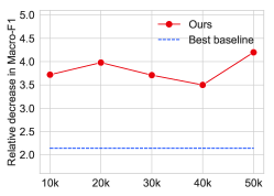
Figure 4: The relative decrease in Macro-F1 score of node-level attacks against GCN with different size of the candidate set on Citeseer dataset. The blue dashed line denotes the performance of the best baseline when candidate size is chosen as $20\text{k}$.

The selection of candidate set. We have mentioned that one limitation of our attack strategy is the randomly selected candidate set, which introduces a further approximation. We here further analyze the impact of the candidate set size. Figure 4 shows the relative decrease when we choose the size of candidate set among $\{10\text{k},20\text{k},30\text{k},40\text{k},50\text{k}\}$. We observe that although our model performs slightly better if we randomly select $50\text{k}$ edge pairs as the candidate, the candidate size appears to have little influence on the overall performance, which partly verifies the practical utility of our strategy of randomly selecting candidates.

Parameter Analysis. Our algorithm involves two hyperparameters: namely, the spatial coefficient $k$ and restart threshold $\tau$. We use grid search to find their suitable values on Cora-ML and present here for reference (see Figure 5). Better performance can be obtained when $k\in\{1,2\}$ and $\tau\leq 0.03$. The observation that our model’s superiority when $k\leq 2$ is consistent with many conclusions of graph over-smoothing problem Li et al. (2018); Klicpera et al. (2019). Remarkably, our model can still achieve relatively good performance (i.e., better than the baseline methods) regardless of how hyperparameters are changed.

Detailed results of Table 2. We further report the detailed results (decrease in Macro-F1 score, Macro-Precision score and Macro-Recall score) with standard deviation of node-level attacks in Table 12.

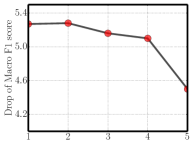
(a) $k$: spatial coefficient

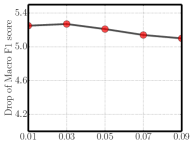
(b) $\tau$: restart threshold

Figure 5: Parameter analysis for node classification task.

References

- Albert and Barabási [2002] Réka Albert and Albert-László Barabási. Statistical mechanics of complex networks. Reviews of Modern Physics, 74:47–97, 2002.
- Bojchevski and Günnemann [2019] Aleksandar Bojchevski and Stephan Günnemann. Adversarial Attacks on Node Embeddings via Graph Poisoning. In ICML, 2019.
- Bollobás [2013] Béla Bollobás. Modern graph theory, volume 184. Springer Science and Business Media, 2013.
- Chang et al. [2020] Heng Chang, Yu Rong, Tingyang Xu, Wenbing Huang, Honglei Zhang, Peng Cui, Wenwu Zhu, and Junzhou Huang. A restricted black-box adversarial framework towards attacking graph embedding models. In AAAI, 2020.
- Chen et al. [2018] Jinyin Chen, Yangyang Wu, Xuanheng Xu, Yixian Chen, Haibin Zheng, and Qi Xuan. Fast Gradient Attack on Network Embedding. ArXiv, 2018.
- Chung [1997] Fan R. K. Chung. Spectral graph theory. American Mathematical Soc., 1997.
- Cohen et al. [2017] Michael B. Cohen, Jonathan Kelner, John Peebles, Richard Peng, Anup B. Rao, Aaron Sidford, and Adrian Vladu. Almost-linear-time algorithms for markov chains and new spectral primitives for directed graphs. In STOC, 2017.
- Dai et al. [2018] Hanjun Dai, Hui Li, Tian Tian, Xin Huang, Lin Wang, Jun Zhu, and Le Song. Adversarial Attack on Graph Structured Data. In ICML, 2018.
- Entezari et al. [2020] Negin Entezari, Saba A Al-Sayouri, Amirali Darvishzadeh, and Evangelos E Papalexakis. All you need is low (rank) defending against adversarial attacks on graphs. In WSDM, 2020.
- Gilmer et al. [2017] Justin Gilmer, Samuel S. Schoenholz, Patrick F. Riley, Oriol Vinyals, and George E. Dahl. Neural Message Passing for Quantum Chemistry. In ICML, 2017.
- Grover and Leskovec [2016] Aditya Grover and Jure Leskovec. Node2vec: Scalable Feature Learning for Networks. In SIGKDD, 2016.
- Gyongyi and Garcia-Molina [2005] Zoltan Gyongyi and Hector Garcia-Molina. Link spam alliances. Technical report, Stanford, 2005.
- Holme and Kim [2002] Petter Holme and Beom Jun Kim. Growing scale-free networks with tunable clustering. Physical Review E, 65(2):026107, 2002.
- Horn and Johnson [2008] Roger A. Horn and Charles R. Johnson. Topics in Matrix Analysis. Cambridge Univ. Press, 2008.
- Jin et al. [2020] Wei Jin, Yaxin Li, Han Xu, Yiqi Wang, and Jiliang Tang. Adversarial attacks and defenses on graphs: A review and empirical study. ArXiv, 2020.
- Kipf and Welling [2017] Thomas N. Kipf and Max Welling. Semi-Supervised Classification with Graph Convolutional Networks. In ICLR, 2017.
- Klicpera et al. [2019] Johannes Klicpera, Aleksandar Bojchevski, and Stephan Günnemann. Predict then propagate: Graph neural networks meet personalized pagerank. In ICLR, 2019.
- Li et al. [2018] Qimai Li, Zhichao Han, Yuriy Wu, and Xiao-Ming. Deeper insights into graph convolutional networks for semi-supervised learning,. In AAAI, 2018.
- Lovász [1993] L. Lovász. Random walks on graphs: A survey. Combinatorics, Paul erdos is eighty, 2(1):1–46, 1993.
- Ma et al. [2020] Jiaqi Ma, Shuangrui Ding, and Qiaozhu Mei. Towards more practical adversarial attacks on graph neural networks. In NeurIPS, 2020.
- Paranjape et al. [2017] Ashwin Paranjape, Austin R. Benson, and Jure Leskovec. Motifs in Temporal Networks. In WSDM, 2017.
- Pei et al. [2015] Yulong Pei, Nilanjan Chakraborty, and Katia Sycara. Nonnegative matrix tri-factorization with graph regularization for community detection in social networks. In IJCAI, 2015.
- Perozzi et al. [2014] Bryan Perozzi, Rami Al-Rfou, and Steven Skiena. DeepWalk: Online learning of social representations. In SIGKDD, 2014.
- Stewart and Sun [1990] G. W. Stewart and Ji-guang Sun. Matrix Perturbation Theory. Computer Science and Scientific Computing. Academic Press, Boston, 1990.
- Veličković et al. [2018] Petar Veličković, Guillem Cucurull, Arantxa Casanova, Adriana Romero, Pietro Lio, and Yoshua Bengio. Graph attention networks. In ICLR, 2018.
- Wang et al. [2018] Xiaoyun Wang, Joe Eaton, Cho-Jui Hsieh, and Shyhtsun Felix Wu. Attack Graph Convolutional Networks by Adding Fake Nodes. ArXiv, 2018.
- Watts and Strogatz [1998] Duncan J. Watts and Steven H. Strogatz. Collective dynamics of ‘small-world’ networks. Nature, 393(6684):440–442, 1998.
- Wu et al. [2019] Huijun Wu, Chen Wang, Yuriy Tyshetskiy, Andrew Docherty, Kai Lu, and Liming Zhu. Adversarial Examples for Graph Data: Deep Insights into Attack and Defense. In IJCAI, 2019.
- Xu et al. [2019a] Kaidi Xu, Hongge Chen, Sijia Liu, Pin-Yu Chen, Tsui-Wei Weng, Mingyi Hong, and Xue Lin. Topology Attack and Defense for Graph Neural Networks: An Optimization Perspective. In IJCAI, 2019.
- Xu et al. [2019b] Keyulu Xu, Weihua Hu, Jure Leskovec, and Stefanie Jegelka. How Powerful are Graph Neural Networks? In ICLR, 2019.
- Ying et al. [2018] Zhitao Ying, Jiaxuan You, Christopher Morris, Xiang Ren, William L. Hamilton, and Jure Leskovec. Hierarchical Graph Representation Learning with Differentiable Pooling. In NeurIPS, 2018.
- Yu et al. [2006] Haifeng Yu, Michael Kaminsky, Phillip B Gibbons, and Abraham Flaxman. Sybilguard: defending against sybil attacks via social networks. In SIGCOMM, 2006.
- Yu et al. [2020] Shanqing Yu, Jun Zheng, Lihong Chen, Jinyin Chen, Qi Xuan, and Qingpeng Zhang. Unsupervised Euclidean Distance Attack on Network Embedding. In DSC, 2020.
- Zhu and Ghahramani [2003] Xiaojin Zhu and Zoubin Ghahramani. Learning from labeled and unlabeled data with label propagation. Technical report, Carneige Mellon University, 07 2003.
- Zügner and Günnemann [2019] Daniel Zügner and Stephan Günnemann. Adversarial Attacks on Graph Neural Networks via Meta Learning. In ICLR, 2019.
- Zügner et al. [2018] Daniel Zügner, Amir Akbarnejad, and Stephan Günnemann. Adversarial Attacks on Neural Networks for Graph Data. In SIGKDD, 2018.