A semigroup method for high dimensional committor functions based on neural network

Abstract

This paper proposes a new method based on neural networks for computing the high-dimensional committor functions that satisfy Fokker-Planck equations. Instead of working with partial differential equations, the new method works with an integral formulation based on the semigroup of the differential operator. The variational form of the new formulation is then solved by parameterizing the committor function as a neural network. There are two major benefits of this new approach. First, stochastic gradient descent type algorithms can be applied in the training of the committor function without the need of computing any mixed second order derivatives. Moreover, unlike the previous methods that enforce the boundary conditions through penalty terms, the new method takes into account the boundary conditions automatically. Numerical results are provided to demonstrate the performance of the proposed method.

1 Introduction

Understanding rare transition events between two states is important for studying the behavior of stochastic systems in physics, chemistry, and biology. One important method to describe the transition events is the transition path theory (Vanden-Eijnden et al., 2010; E and Vanden-Eijnden, 2006; Lu and Nolen, 2015), and the central object in the transition path theory is the committor function. Assume that the transition between two states is governed by the overdamped Langevin process

$$d\mathbf{x}_{t}=-\nabla V\left(\mathbf{x}_{t}\right)dt+\sqrt{2\beta^{-1}}d\mathbf{w}_{t},$$ (1)

where $\mathbf{x}_{t}\in\Omega\subset\mathbb{R}^{d}$ is the state of the system, $V:\mathbb{R}^{d}\rightarrow\mathbb{R}$ is a smooth potential function, $\beta=1/T$ is the inverse of the temperature $T$, and $\mathbf{w}_{t}$ is the standard $d$-dimensional Brownian motion. For two given simply connected domains $A$ and $B$ in $\Omega$ with smooth boundaries, the committor function $q(\mathbf{x})$ is defined as

$$q(\mathbf{x})=\mathbb{P}(\tau_{B}<\tau_{A}\mid\mathbf{x}_{0}=\mathbf{x}),$$ (2)

where $\tau_{A}$ and $\tau_{B}$ are the hitting times for the sets $A$ and $B$, respectively. Many statistical properties of the transition are encoded in the committor function.

The committor function satisfies the Fokker-Planck equation (also known as the steady-state backward Kolmogorov equation)

$$(-1/\beta\Delta+\nabla V\cdot\nabla)q=0\text{in}\Omega\backslash(A\cup B),\quad\left.q(\mathbf{x})\right|_{\partial A}=0,\quad\left.q(\mathbf{x})\right|_{\partial B}=1.$$ (3)

If the potential $V$ is confining, i.e. $V(\mathbf{x})\rightarrow\infty$ as $|\mathbf{x}|\rightarrow\infty$ and the partition function $Z_{\beta}=\int_{\mathbb{R}^{d}}\exp(-\beta V(\mathbf{x}))d\mathbf{x}<\infty$ for any $\beta>0$, then

$$\rho(\mathbf{x})=\frac{1}{Z_{\beta}}\exp(-\beta V(\mathbf{x}))$$ (4)

is the equilibrium distribution of the Langevin dynamics langevin. Under this condition, the Langevin process langevin is ergodic (Pavliotis, 2014), which enables the use of Monte Carlo methods to sample from the equilibrium distribution. For the rest of the paper we will always assume that $V$ is confining and $\rho$ exists.

One major difficulty in solving committor is the curse of dimensionality. Various methods have been proposed under the assumption that the transition from $A$ to $B$ is concentrated in a quasi-one dimensional tube or low dimensional manifold. For example, the finite temperature string method (E et al., 2005; Vanden-Eijnden and Venturoli, 2009) approximates isosurfaces of the committor function with hyperplanes normal to the most probable transition paths, and updates the transition paths together with the isocommittor-surfaces. Diffusion map (Coifman et al., 2008) solves for $q$ on a set of points by applying point cloud discretization to the operator $L=(-1/\beta\Delta+\nabla V\cdot\nabla)$. In order to obtain better convergence order, (Lai and Lu, 2018) improves on diffusion map by discretizing $L$ using a finite element method on local tangent planes of the point cloud.

More recently, the method proposed in (Khoo et al., 2019) works with the variational form of the Fokker-Planck equation

$$\underset{q}{\operatorname{argmin}}\int_{\Omega\backslash(A\cup B)}|\nabla q(\mathbf{x})|^{2}\rho(\mathbf{x})d\mathbf{x},\left.\quad q(\mathbf{x})\right|_{\partial A}=0,\left.\quad q(\mathbf{x})\right|_{\partial B}=1,$$ (5)

and parameterizes the high-dimensional committor function $q(\cdot)$ by a neural network (NN) $q_{\theta}(\cdot)$. The main advantage of working with an optimization formulation is that under rather mild conditions stochastic gradient descent (SGD) type algorithms can avoid the saddle points and converge efficiently to at least local minimums, as shown for example in Jin et al. (2019). The boundary conditions can be enforced by additional penalty terms as in

$$\aligned\underset{\theta\in\mathbb{R}^{p}}{\operatorname{argmin}}\int_{\text{\hbox to10.0pt{$\Omega\backslash(A\cup B)$\hss\hss}}}\left|\nabla q_{\theta}(\mathbf{x})\right|^{2}\rho(\mathbf{x})d\mathbf{x}+\tilde{c}\int_{\partial A}q_{\theta}(\mathbf{x})^{2}dm_{\partial A}(\mathbf{x})+\tilde{c}\int_{\partial B}\left(q_{\theta}(\mathbf{x})-1\right)^{2}dm_{\partial B}(\mathbf{x}),$$ (6)

where $m_{A}$ and $m_{B}$ are measures supported on $\partial A$ and $\partial B$. The integral in weakpenalty is approximated by a Monte-Carlo method where the samples are generated according to the stochastic process langevin. Satisfactory numerical results are obtained with this method even in high dimensional cases where traditional methods like finite-element-type methods are intractable. However, because the loss depends on $|\nabla q_{\theta}|^{2}$, obtaining the gradient of the loss with respect to $\theta$ requires an inconvenient second order derivative computation.

The contribution of this paper is two-fold. First, we propose a new method that removes the dependence on the second order derivatives by working with an integral formulation based on the semigroup of langevin. Second, the boundary conditions are treated automatically by the semigroup formulation rather than relying solely on the penalty terms, which makes it easier to tune the penalty coefficients. The paper is organized as follows. Section 2 describes the new formulation and the neural network approximation. Section 3 analyzes this new method under the so-called lazy-training regime. Finally, the performance of our method is examined numerically in Section 4.

2 Proposed method

2.1 A new variational formulation

Consider the Langevin process starting from a point $\mathbf{x}\in\Omega$

$$\aligned d\mathbf{x}_{t}&=-\nabla V\left(\mathbf{x}_{t}\right)dt+\sqrt{2\beta^{-1}}d\mathbf{w}_{t},\\ \mathbf{x}_{0}=\mathbf{x}.$$ (7)

Let $\tau_{A}$ and $\tau_{B}$ be the stopping time of the process hitting $\partial A$ and $\partial B$, respectively. Similarly, define $\tau\equiv\tau_{A\cup B}=\min(\tau_{A},\tau_{B})$ be the hitting time of $A\cup B$. For a fixed small time step $\delta>0$, we define the operator $P$ as follows:

$$(Pf)(\mathbf{x}):=\mathbb{E}^{\mathbf{x}}\left(f\left(\mathbf{x}_{\tau\wedge\delta}\right)\right),$$ (8)

where $\mathbb{E}^{\mathbf{x}}$ is the expectation taken with respect to the law of the process eq:trajectory.

Proposition

When $\nabla V$ is bounded and Lipschitz continuous on $\mathbb{R}^{d}$, the solution to the committor function committor satisfies the following semigroup formulation

$$q(\mathbf{x})=(Pq)(\mathbf{x})\quad\text{in}\quad\Omega\backslash(A\cup B),\quad q|_{\partial A}=0,\quad q|_{\partial B}=1.$$ (9)

The proof of Proposition 2.1 is provided in Appendix A. The main advantage of working with eq:justifiedreplace over committor is that it does not contain any differential operator.

For notational convenience, we introduce a function $r:\partial A\cup\partial B\rightarrow\mathbb{R}$ with $r(\mathbf{x})|_{\partial A}=0$ and $r(\mathbf{x})|_{\partial B}=1$. With this definition, the boundary condition of eq:justifiedreplace is simply $q=r$ on $\partial A\cup\partial B$. In order to introduce the variational formulation, $Pq$ can be split into two parts as follows:

$$\aligned(Pq)(\mathbf{x})&=\mathbb{E}^{\mathbf{x}}\left(q\left(\mathbf{x}_{\tau\wedge\delta}\right)\right)=\mathbb{E}^{\mathbf{x}}\left(q\left(\mathbf{x}_{\tau\wedge\delta}\right)\mathbf{1}_{\{\delta<\tau\}}\right)+\mathbb{E}^{\mathbf{x}}\left(q\left(\mathbf{x}_{\tau\wedge\delta}\right)\mathbf{1}_{\{\delta\geq\tau\}}\right)\\ =\mathbb{E}^{\mathbf{x}}\left(q\left(\mathbf{x}_{\delta}\right)\mathbf{1}_{\{\delta<\tau\}}\right)+\mathbb{E}^{\mathbf{x}}\left(q\left(\mathbf{x}_{\tau}\right)\mathbf{1}_{\{\delta\geq\tau\}}\right)\\ =\mathbb{E}^{\mathbf{x}}\left(q\left(\mathbf{x}_{\delta}\right)\mathbf{1}_{\{\delta<\tau\}}\right)+\mathbb{E}^{\mathbf{x}}\left(r\left(\mathbf{x}_{\tau}\right)\mathbf{1}_{\{\delta\geq\tau\}}\right),$$ (10)

where the last equality results from the fact that $\mathbf{x}_{\tau}\in\partial A\cup\partial B$ and $q=r$ on $\partial A\cup\partial B$.

We denote the first part of eq:split as

$$(P^{i}q)(\mathbf{x})\equiv\mathbb{E}^{\mathbf{x}}\left(q(\mathbf{x}_{\tau\wedge\delta})\mathbf{1}_{\{\delta<\tau\}}\right)=\mathbb{E}^{\mathbf{x}}\left(q(\mathbf{x}_{\delta})\mathbf{1}_{\{\delta<\tau\}}\right),$$ (11)

where the superscript $i$ stands for the interior contribution and the second part of eq:split as

$$(P^{b}r)(\mathbf{x})\equiv\mathbb{E}^{\mathbf{x}}\left(r(\mathbf{x}_{\tau\wedge\delta})\mathbf{1}_{\{\delta\geq\tau\}}\right)=\mathbb{E}^{\mathbf{x}}\left(r(\mathbf{x}_{\tau})\mathbf{1}_{\{\delta\geq\tau\}}\right),$$ (12)

where the superscript $b$ stands for the boundary contribution. With these definitions, we can rewrite eq:justifiedreplace compactly as

$$(I-P^{i})q(\mathbf{x})-(P^{b}r)(\mathbf{x})=0,$$ (13)

where $I$ is the identity operator. The following result states that $P^{i}$ is symmetric on the Hilbert space $L_{\rho}^{2}(\Omega\backslash(A\cup B))$.

Proposition

$P^{i}$ is a symmetric operator on $L_{\rho}^{2}(\Omega\backslash(A\cup B))$, in other words, $\langle u,P^{i}v\rangle_{\rho}=\langle P^{i}u,v\rangle_{\rho}$, where $\langle\cdot,\cdot\rangle_{\rho}$ denotes the inner product of the Hilbert space $L_{\rho}^{2}(\Omega\backslash(A\cup B))$.

For the proof of this proposition, see Appendix B.

Based on Proposition 2.1, we are now ready to propose the following variational formulation for eq:nobd

$$\aligned\min_{q}\frac{1}{2}\int_{\text{\hbox to10.0pt{$\Omega\backslash(A\cup B)$\hss\hss}}}q(\mathbf{x})\left((I-P^{i})q(\mathbf{x})\right)\rho(\mathbf{x})d\mathbf{x}-\int_{\text{\hbox to10.0pt{$\Omega\backslash(A\cup B)$\hss\hss}}}q(\mathbf{x})P^{b}r(\mathbf{x})\rho(\mathbf{x})d\mathbf{x}$$ (14)

The two formulations eq:variational and eq:nobd share the same solution as shown below. Let $q^{*}$ be the solution to the variational problem eq:variational and $q(\mathbf{x},\epsilon)=q^{*}(\mathbf{x})+\epsilon\eta(\mathbf{x})$, where $\eta$ is continuous with compact support. By taking derivative with respect to $\epsilon$ at $\epsilon=0$ we obtain

$$\aligned 0&=\frac{\partial}{\partial\epsilon}\left.\left(\frac{1}{2}\int_{\text{\hbox to10.0pt{$\Omega\backslash(A\cup B)$\hss\hss}}}q(\mathbf{x},\epsilon)\left((I-P^{i})q(\mathbf{x},\epsilon)\right)\rho(\mathbf{x})d\mathbf{x}-\int_{\text{\hbox to10.0pt{$\Omega\backslash(A\cup B)$\hss\hss}}}q(\mathbf{x},\epsilon)P^{b}r(\mathbf{x})\rho(\mathbf{x})d\mathbf{x}\right)\right|_{\epsilon=0}\\ =\int_{\text{\hbox to10.0pt{$\Omega\backslash(A\cup B)$\hss\hss}}}\eta(\mathbf{x})\left((I-P^{i})q^{*}(\mathbf{x})\right)\rho(\mathbf{x})d\mathbf{x}-\int_{\text{\hbox to10.0pt{$\Omega\backslash(A\cup B)$\hss\hss}}}\eta(\mathbf{x})P^{b}r(\mathbf{x})\rho(\mathbf{x})d\mathbf{x}\\ =\int_{\text{\hbox to10.0pt{$\Omega\backslash(A\cup B)$\hss\hss}}}\eta(\mathbf{x})\left((I-P^{i})q^{*}(\mathbf{x})-P^{b}r(\mathbf{x})\right)\rho(\mathbf{x})d\mathbf{x},$$ (15)

where the second equality uses Proposition 2.1. Since this is true for any continuous $\eta$ with compact support and $\rho(\mathbf{x})>0$, we conclude that $(I-P^{i})q^{*}(\mathbf{x})-P^{b}r(\mathbf{x})=0$ on $\Omega\backslash(A\cup B)$.

Plugging in the definitions of $P^{i}$ and $P^{b}$ into eq:variational leads to

$$\aligned\min_{q}~{}\frac{1}{2}\int_{\text{\hbox to10.0pt{$\Omega\backslash(A\cup B)$\hss\hss}}}q(\mathbf{x})\left(q(\mathbf{x})-\mathbb{E}^{\mathbf{x}}\left(q\left(\mathbf{x}_{\delta}\right)\mathbf{1}_{\{\delta<\tau\}}\right)\right)\rho(\mathbf{x})d\mathbf{x}-\int_{\text{\hbox to10.0pt{$\Omega\backslash(A\cup B)$\hss\hss}}}q(\mathbf{x})\mathbb{E}^{\mathbf{x}}\left(r\left(\mathbf{x}_{\tau}\right)\mathbf{1}_{\{\delta\geq\tau\}}\right)\rho(\mathbf{x})d\mathbf{x}.$$ (16)

It is clear from this formulation that there is no need for taking gradient of $q(\mathbf{x})$ with respect to $\mathbf{x}$.

Although there is no need to enforce the boundary conditions $q|_{\partial A}=0$ and $q|_{\partial B}=1$ explicitly in eq:variational, one can still include the penalty terms that can sometimes give a better performance

$$\aligned\min_{q}\frac{1}{2}&\int_{\text{\hbox to10.0pt{$\Omega\backslash(A\cup B)$\hss\hss}}}q(\mathbf{x})\left((I-P^{i})q(\mathbf{x})\right)\rho(\mathbf{x})d\mathbf{x}-\int_{\text{\hbox to10.0pt{$\Omega\backslash(A\cup B)$\hss\hss}}}q(\mathbf{x})P^{b}r(\mathbf{x})\rho(\mathbf{x})d\mathbf{x}\\ +\frac{c}{2}\int_{\partial A}q(\mathbf{x})^{2}dm_{A}(\mathbf{x})+\frac{c}{2}\int_{\partial B}(q(\mathbf{x})-1)^{2}dm_{B}(\mathbf{x}),$$ (17)

where $m_{A}$ and $m_{B}$ are measures supported on $\partial A$ and $\partial B$, respectively, and $c>0$ is a penalty constant.

2.2 Nonlinear parameterization

In order to deal with the high dimensionality of the committor function $q(\mathbf{x})$, we propose to approximate $q(\mathbf{x})$ with an NN $q_{\theta}(\mathbf{x})$, where $\theta$ stands for the NN parameters. In terms of $\theta$, the optimization problem takes the form

$$\aligned\min_{\theta}\frac{1}{2}&\int_{\text{\hbox to10.0pt{$\Omega\backslash(A\cup B)$\hss\hss}}}q_{\theta}(\mathbf{x})\left((I-P^{i})q_{\theta}(\mathbf{x})\right)\rho(\mathbf{x})d\mathbf{x}-\int_{\text{\hbox to10.0pt{$\Omega\backslash(A\cup B)$\hss\hss}}}q_{\theta}(\mathbf{x})P^{b}r(\mathbf{x})\rho(\mathbf{x})d\mathbf{x}\\ +\frac{c}{2}\int q_{\theta}(\mathbf{x})^{2}dm_{A}(\mathbf{x})+\frac{c}{2}\int(q_{\theta}(\mathbf{x})-1)^{2}dm_{B}(\mathbf{x}).$$ (18)

When applying an stochastic gradient descent (SGD) to optimize eq:no gradient var, one needs to compute the derivative for each of the terms.

Derivative of the first two terms.

By the symmetric property stated in Proposition 2.1, the derivative of the first two terms of eq:no gradient var is

$$\aligned&\int_{\text{\hbox to10.0pt{$\Omega\backslash(A\cup B)$\hss\hss}}}\nabla_{\theta}q_{\theta}(\mathbf{x})\left((I-P^{i})q_{\theta}(\mathbf{x})\right)\rho(\mathbf{x})d\mathbf{x}-\int_{\text{\hbox to10.0pt{$\Omega\backslash(A\cup B)$\hss\hss}}}\nabla_{\theta}q_{\theta}(\mathbf{x})P^{b}r(\mathbf{x})\rho(\mathbf{x})d\mathbf{x}\\ =\int_{\text{\hbox to10.0pt{$\Omega\backslash(A\cup B)$\hss\hss}}}\nabla_{\theta}q_{\theta}(\mathbf{x})\left(q_{\theta}(\mathbf{x})-\mathbb{E}^{\mathbf{x}}\left(q_{\theta}(\mathbf{x}_{\delta})\mathbf{1}_{\{\delta<\tau\}}\right)-\mathbb{E}^{\mathbf{x}}\left(g(\mathbf{x}_{\tau})\mathbf{1}_{\{\delta\geq\tau\}}\right)\right)\rho(\mathbf{x})d\mathbf{x}.$$ (19)

Notice that $\eqref{eq:derivative1}$ is an integral with measure $\rho(\mathbf{x})d\mathbf{x}$. Therefore, if $\mathbf{x}\sim\rho$ and $\mathbf{x}_{\delta}$ follows eq:trajectory, eq:derivative1 can be written as

$$\mathbb{E}_{\mathbf{x}\sim\rho}\nabla_{\theta}q_{\theta}(\mathbf{x})\left(q_{\theta}(\mathbf{x})-\mathbb{E}^{\mathbf{x}}\left(q_{\theta}\left(\mathbf{x}_{\delta}\right)\mathbf{1}_{\{\delta<\tau\}}\right)-\mathbb{E}^{\mathbf{x}}\left(r(\mathbf{x}_{\tau})\mathbf{1}_{\{\delta\geq\tau\}}\right)\right).$$ (20)

An unbiased estimator for eq:derivative1 in an SGD method is therefore

$$\nabla_{\theta}q_{\theta}(\mathbf{x})\left(q_{\theta}(\mathbf{x})-q_{\theta}(\mathbf{x}_{\delta})\mathbf{1}_{\{\delta<\tau\}}-r(\mathbf{x}_{\tau})\mathbf{1}_{\{\delta\geq\tau\}}\right)=\nabla_{\theta}q_{\theta}(\mathbf{x})\left(q_{\theta}(\mathbf{x})-q_{\theta}(\mathbf{x}_{\delta})\mathbf{1}_{\{\delta<\tau\}}-\mathbf{1}_{\{\delta\geq\tau=\tau_{B}\}}\right).$$ (21)

The significance of eq:unbiased is that one only needs to take the gradient once with respect to the parameter $\theta$, whereas in (Khoo et al., 2019) one needs to take the gradient of both $\mathbf{x}$ and $\theta$.

Let us comment on the implementation details of eq:unbiased. First, the sample $\mathbf{x}$ is supposed to be sampled from $\rho$. As mentioned previously, if the potential function $V$ is confining, then the Langevin process langevin is ergodic. This implies that the distribution of the samples $\mathbf{x}_{t}$ generated from the stochastic differential equation (SDE) eq:trajectory converges to $\rho$ in the limit of $t\rightarrow\infty$. Therefore, after an initial burn-in period, the samples from the SDE trajectory follow the distribution $\rho$. There has been a large literature on how to solve SDE eq:trajectory numerically. The simplest method is the Euler-Maruyama scheme (see for example (Kloeden and Platen, 2013)). Let $\Delta t>0$ be the time step size and $\mathbf{w}_{\Delta t}\sim\mathcal{N}(0,{\Delta t}I_{d})$, and $I_{d}$ is the $d$-dimensional identity matrix. The Euler-Maruyama approximation $\tilde{\mathbf{x}}_{n\Delta t}$ at time steps $n\Delta t$ are computed via

$$\tilde{\mathbf{x}}_{(n+1)\Delta t}=\tilde{\mathbf{x}}_{n\Delta t}-\nabla{V}(\tilde{\mathbf{x}}_{n\Delta t})\Delta t+\sqrt{2\beta^{-1}}\mathbf{w}_{\Delta t}.$$

Assuming ergodicity, the distribution $\mathbf{x}\sim\rho$ can be approximated by $\tilde{\mathbf{x}}_{N\Delta t}$ for a sufficiently small $\Delta t$ and sufficiently large $N$ with an arbitrary $\tilde{\mathbf{x}}_{0}$.

Second, given $\mathbf{x}\sim\rho$, one needs to sample $\mathbf{x}_{\delta}$. We approximate $\mathbf{x}_{\delta}$ by Euler-Maruyama scheme as well

$$\mathbf{x}_{\delta}=\mathbf{x}-\nabla{V}(\mathbf{x})\delta+\sqrt{2\beta^{-1}}\mathbf{w}_{\delta},$$ (22)

where $\mathbf{w}_{\delta}\sim\mathcal{N}(0,\delta I_{d})$.

Finally, it is necessary to determine the indicators $\mathbf{1}_{\{\delta<\tau\}}$, $\mathbf{1}_{\{\delta\geq\tau=\tau_{A}\}}$ and $\mathbf{1}_{\{\delta\geq\tau=\tau_{B}\}}$ in order to compute eq:unbiased. For this, the following approximations are used

$$\mathbf{1}_{\{\delta<\tau\}}=1\;\text{if}\;\mathbf{x}_{\delta}\in\Omega\backslash A\cup B,\quad\mathbf{1}_{\{\delta\geq\tau=\tau_{A}\}}=1\;\text{if}\;\mathbf{x}_{\delta}\in A,\quad\mathbf{1}_{\{\delta\geq\tau=\tau_{B}\}}=1\;\text{if}\;\mathbf{x}_{\delta}\in B.$$

Intuitively these approximations should work well when $\delta$ is sufficiently small, which is also supported by the numerical experiments. Even for a fixed $\delta$, we can apply Euler-Maruyama scheme with multiple steps to improve the accuracy. Specifically, given $\mathbf{x}\sim\rho$, one can approximate $\mathbf{x}_{\delta}$ by the last term of the sequence $\mathbf{x}_{0},\mathbf{x}_{\delta/M},\ldots,\mathbf{x}_{\delta}$, where

$$\mathbf{x}_{(k+1)\delta/M}=\mathbf{x}_{k\delta/M}-\nabla{V}(\mathbf{x}_{k\delta/M})\delta/M+\sqrt{2\beta^{-1}}\mathbf{w}_{\delta/M},$$ (23)

and $\mathbf{x}_{0}=\mathbf{x}$. When using the multiple-step approximation, the indicators are determined by

$$\aligned\mathbf{1}_{\{\delta<\tau\}}&=1\;\text{if}\;\{\mathbf{x}_{k\delta/M}\}_{k=1}^{M}\subset\Omega\backslash A\cup B,\\ \mathbf{1}_{\{\delta\geq\tau=\tau_{A}\}}=1\;\text{if}\;\{\mathbf{x}_{k\delta/M}\}_{k=1}^{M}\cap A\not=\emptyset,\\ \mathbf{1}_{\{\delta\geq\tau=\tau_{B}\}}=1\;\text{if}\;\{\mathbf{x}_{k\delta/M}\}_{k=1}^{M}\cap B\not=\emptyset.$$

It is worth mentioning that various importance sampling methods (see for example (Li et al., 2019; Rotskoff and Vanden-Eijnden, 2020)) can potentially be used to approximate the integral in eq:MCint and the corresponding gradients calculated above. One can generate the initial state $\mathbf{x}$ in eq:nextstep using importance sampling techniques, and then generate $\mathbf{x}_{\delta}$ and also subsequent samples according to eq:nextstep.

Derivative of the penalty terms.

For the third and fourth terms of eq:no gradient var, unbiased estimators of their gradients are

$$c\nabla_{\theta}q_{\theta}(\mathbf{x}_{A})q_{\theta}(\mathbf{x}_{A}),\quad c\nabla_{\theta}q_{\theta}(\mathbf{x}_{B})(q_{\theta}(\mathbf{x}_{B})-1),$$ (24)

respectively, where $\mathbf{x}_{A}\sim m_{A}$ and $\mathbf{x}_{B}\sim m_{B}$.

Connection with reinforcement learning.

Solving committor function can be viewed as a special case of the policy evaluation problem in reinforcement learning (RL): $\Omega\backslash(A\cup B)$ is the state space; the transition kernel is given by the operator $P^{i}$ defined in eq:pi; the discount factor is equal to one; there is no immediate reward for each individual step but the final reward is $(P^{b}g)(\mathbf{x})$; $q(\mathbf{x})$ is the value function of the problem; eq:nobd is the Bellman equation; and eq:unbiased is the temporal difference (TD) update.

However, the key difference with the general policy evaluation problem is that, due to the detailed balancing of overdamped Langevin dynamics, there is a variational formulation eq:variational for eq:nobd, which is not available for general RL problems except the special case considered in (Ollivier, 2018). Because of the variational formulation, eq:unbiased is guaranteed to converge at least to a local minimum, even in the neural network parameterization. On the other hand, such a stability result fails to exist for neural network approximations for general RL problems, as many techniques and tricks are required in order for the neural network parameters to converge.

2.3 Neural network architecture

The architecture of the neural network $q_{\theta}(\mathbf{x})$ follows the one used in (Khoo et al., 2019) and is specifically designed for this problem. Below we briefly summarize the main design considerations.

In the low temperature regime, i.e. when $T\rightarrow 0$, there is typically a sharp interface between $A$ and $B$, as pointed out by (Khoo et al., 2019). In order to account for this sharp transition, the tangent function $\tanh$ is used as the activation function at the last nonlinear layer, as shown in Fig. 1.

In the high temperature regime, i.e. when $T\rightarrow\infty$, there is another type of singular behavior. As $T\rightarrow\infty$, the equation committor converges heuristically to a Laplace equation with a Dirichlet boundary condition. When the domains $A$ and $B$ are relatively small, the solution near the boundary $\partial A$ and $\partial B$ are dictated asymptotically by the fundamental solution

$$\Phi(\mathbf{x}):=\left\{\begin{array}[]{ll}-\frac{1}{2\pi}\log|\mathbf{x}|&(n=2)\\ \frac{\Gamma(n/2)}{(2\pi)^{n/2}|\mathbf{x}|^{n-2}}&(n\geq 3)\end{array}\right.,$$ (25)

where $n$ is the inherent dimension of the Laplace equation of $T\rightarrow\infty$, as demonstrated in (Khoo et al., 2019). For example, in the rugged-Muller problem 4.2, the inherent dimension $n=2$, while in the Ginzburg-Landau problem 4.3 we have $n=d=49$.

In order to address these two types of singular behaviors, we introduce the following parameterization

$$q_{\theta}(\mathbf{x}):=n_{\theta_{A}}(\mathbf{x})S_{A}\left(\mathbf{x}-\mathbf{y}^{A}\right)+n_{\theta_{B}}(\mathbf{x})S_{B}\left(\mathbf{x}-\mathbf{y}^{B}\right)+n_{\theta_{0}}(\mathbf{x}),$$ (26)

where $\mathbf{y}^{A}$ and $\mathbf{y}^{B}$ are the centers of $A$ and $B$, $S_{A}(\mathbf{x}-\mathbf{y})$ and $S_{B}(\mathbf{x}-\mathbf{y})$ are set to be fundamental solutions eq:fund, with $n$ depending on the inherent dimension of the problem. Finally, $n_{\theta_{A}}$, $n_{\theta_{B}}$ are fully connected neural networks with ReLU activation, and $n_{\theta_{0}}$ is a fully connected neural network with $\tanh$ activation at the last nonlinear layer and ReLU activation at other nonlinear layers. This architecture is summarized in Fig. 1.

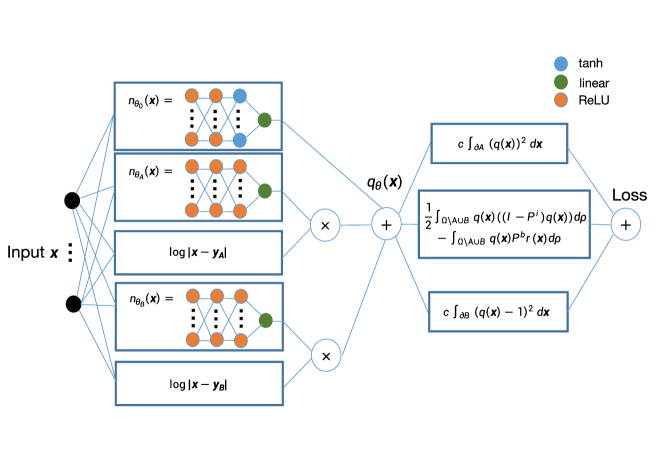
Figure 1: An example of the neural network architecture for a committor function and the corresponding loss. In this example we have two $\log|\mathbf{x}-\mathbf{y}|$ type singularities.

3 Lazy training analysis of the optimization

When the learning rate approaches zero, the dynamics of the SGD can be approximated by the corresponding gradient flow (see (Kushner and Yin, 2003) for example):

$$\theta^{\prime}(t)=-\nabla_{\theta}R(q_{\theta}),\quad\theta(0)=\theta_{0},$$ (27)

where in our case the loss function $R(\cdot)$ takes the form

$$R(q)=\frac{1}{2}\langle(I-P^{i})q-P^{b}r,q\rangle_{\rho}+\frac{c}{2}\langle q,q\rangle_{m_{A}}+\frac{c}{2}\langle q-1,q-1\rangle_{m_{B}},$$ (28)

with $\langle u,v\rangle_{m_{A}}=\int uvdm_{A}$ and $\langle u,v\rangle_{m_{B}}=\int uvdm_{B}$. In this section, we consider instead the rescaled gradient flow

$$\theta^{\prime}(t)=-\frac{1}{\alpha^{2}}\nabla_{\theta}R(\alpha q_{\theta}),\quad\theta(0)=\theta_{0},$$ (29)

with $R(\alpha q)=\frac{1}{2}\langle(I-P^{i})(\alpha q)-P^{b}r,\alpha q\rangle_{\rho}+\frac{c}{2}\langle\alpha q,\alpha q\rangle_{m_{A}}+\frac{c}{2}\langle\alpha q-1,\alpha q-1\rangle_{m_{B}}$, and analyze the training dynamics of $q_{\theta}$ in the lazy training regime. The reason for considering this rescaled formula is that the scaling effect caused by $\alpha$ arises in several situations, for example, when the weights of the NN are large in magnitude at initialization and the learning rate is small (see for example, (Chizat et al., 2019; Agazzi and Lu, 2020)).

In (Chizat et al., 2019), it has been shown that when the scaling factor $\alpha$ is sufficiently large, the gradient flow eq:scaledgf converges at a geometric rate to a local minimum of $F_{\alpha}(\theta)\equiv R(\alpha q_{\theta})/\alpha^{2}$, under some conditions that are detailed below.

Theorem 3.1.

(Chizat et al., 2019) Assume that: (1) $\theta\mapsto q_{\theta}\in\mathcal{F}$, where $\mathcal{F}$ is a separable Hilbert space; (2) $q$ is differentiable with a locally Lipschitz differential $\nabla_{\theta}q_{\theta}$; (3) $q_{\theta_{0}}=0$ and $\operatorname{rank}\nabla_{\theta}q_{\theta}$ is a constant in a neighborhood of $\theta_{0}$; (4) $R$ is strongly convex and differentiable with a Lipschitz gradient.

Then there exists $\alpha_{0}>0$, such that for any $\alpha>\alpha_{0}$, the gradient flow eq:scaledgf converges at a geometric rate to a local minimum of $F_{\alpha}$.

In our setting, $\mathcal{F}$ is the separable Hilbert space $L_{\nu}^{2}((\Omega\backslash(A\cup B))\cup\partial A\cup\partial B)$, where $\nu=\rho+cm_{A}+cm_{B}$ and the rescaled gradient flow is given by

$$\aligned\theta^{\prime}(t)=-\frac{1}{\alpha}\Big{[}&\langle(I-P^{i})\alpha q_{\theta(t)}-P^{b}r,\nabla_{\theta}q_{\theta(t)}\rangle_{\rho}-c\langle\alpha q_{\theta(t)},\nabla_{\theta}q_{\theta(t)}\rangle_{m_{A}}-c\langle\alpha q_{\theta(t)}-1,\nabla_{\theta}q_{\theta(t)}\rangle_{m_{B}}\Big{]}.$$ (30)

The following result states the strong convexity of $R$.

Proposition 1.

Assume that the operator $P^{i}$ defined in eq:pi has a corresponding probability density function $p^{i}(\mathbf{x},\mathbf{y})$ such that

$$P^{i}f(\mathbf{x})=\int_{\text{\hbox to10.0pt{$\Omega\backslash(A\cup B)$\hss\hss}}}p^{i}(\mathbf{x},\mathbf{y})f(\mathbf{y})d\mathbf{y},$$ (31)

and

$$\iint_{\text{\hbox to10.0pt{$\Omega\backslash(A\cup B)\times\Omega\backslash(A\cup B)$\hss\hss}}}p^{i}(\mathbf{x},\mathbf{y})p^{i}(\mathbf{y},\mathbf{x})d\mathbf{x}d\mathbf{y}<\infty.$$ (32)

Then the quadratic form $f\mapsto\langle f,(I-P^{i})f\rangle_{\rho}$ is strongly convex on $L_{\rho}^{2}(\Omega\backslash A\cup B)$.

Based on Proposition 1, the following theorem is a direct consequence of Theorem 3.1.

Theorem 3.2.

Assume that eq:pdf and eq:HS hold, and $q_{\theta_{0}}=0$, and that $\operatorname{rank}\nabla_{\theta}q_{\theta}$ is a constant in a neighborhood of $\theta_{0}$, then there exists $\alpha_{0}>0$, such that for any $\alpha>\alpha_{0}$, the gradient flow eq:gradflow

converges at a geometric rate to a local minimum of $F_{\alpha}(\theta)=R(\alpha q_{\theta})/\alpha^{2}$.

4 Numerical experiments

This section presents the numerical results of the proposed method on several examples. The neural network architecture follows Fig. 1 and the stochastic gradient is computed following the description in Section 2.2. The training is carried out with the Adam optimizer (Kingma and Ba, 2014). Whenever the true solution $q^{*}$ is available, the performance is evaluated by the relative error metric:

$$E=\frac{\|q_{\theta}-q^{*}\|_{L_{\rho}^{2}(\Omega\backslash A\cup B)}}{\|q^{*}\|_{L_{\rho}^{2}(\Omega\backslash A\cup B)}}$$ (33)

computed on a validation dataset generated according to the distribution $\rho$. In all the experiments, $2000$ samples are used for the boundary measures $m_{A}$ and $m_{B}$.

4.1 The double-well potential

In this experiment, consider the committor function in the following double-well potential:

$$V(\mathbf{x})=\left(x_{1}^{2}-1\right)^{2}+0.3\sum_{i=2}^{d}x_{i}^{2},$$ (34)

with $d=10$ and the regions $A$ and $B$ defined as

$$A=\left\{x\in\mathbb{R}^{d}\mid x_{1}\leq-1\right\},\quad B=\left\{x\in\mathbb{R}^{d}\mid x_{1}\geq 1\right\}.$$ (35)

The true solution can be easily obtained by letting $q(\mathbf{x})=\tilde{q}(x_{1})$, such that it satisfies the one-dimensional ordinary differential equation (ODE)

$$\frac{d^{2}\tilde{q}(x_{1})}{dx_{1}^{2}}-4\beta x_{1}(x_{1}^{2}-1)\frac{d\tilde{q}(x_{1})}{dx_{1}}=0,\quad\tilde{q}(0)=0,\quad\tilde{q}(1)=1.$$ (36)

By solving this ODE numerically, we obtain a highly accurate approximation of the exact solution $q^{*}$.

Since the solution of this problem does not exhibit any singular behavior at the boundaries $\partial A$ and $\partial B$, $S_{A}(\cdot)=S_{B}(\cdot)=0$ and the training is only performed for the component $n_{\theta_{0}}(\cdot)$ in eq:NNpara. The problem is solved for the temperatures $T=0.5$ and $T=0.2$. Table 1 summarizes the numerical results and the training parameters. Notice that when the temperature $T$ is lower, the distribution $\rho$ is sparser in $\Omega\backslash(A\cup B)$. Therefore, more samples are used for $T=0.2$ than for $T=0.5$ in order to achieve a comparable precision. For example, for $T=0.5$, $1.5\times 10^{5}$ samples are used for $\Omega\backslash(A\cup B)$ and the relative error is $E=0.014$. On the other hand, for $T=0.2$, $8.0\times 10^{5}$ samples are used and the relative error of the neural network solution is $E=0.011$.

$T$	$E$	$\delta$	$c$	No. training samples	Batch size	No. testing samples
0.5	0.014	$0.003$	15	$1.5\times 10^{5}$	$1000$	$4.0\times 10^{5}$
0.2	0.011	$0.003$	15	$8.0\times 10^{5}$	$1000$	$8.0\times 10^{5}$

Table 1: Results for the double-well potential problem.

The numerical solution for $T=0.5$ is shown in Fig. 2. The committor function $q_{\theta}$ represented by a neural network and the committor function $q^{*}$ obtained via solving eq:ode are plotted along the $x_{1}$ dimension for a fixed $(x_{2},\ldots,x_{d})$. The plot demonstrates that the NN committor function gives a satisfactory approximation to the true solution. We comment here that the final error is not sensitive to the parameter $\delta$. For example, for the case with $T=0.5$, $\delta=0.003$ is used. If $\delta=0.01,0.03,0.05$ are chosen instead, the corresponding final errors are $E=0.013,0.013,0.013$, respectively. We also comment that using the multi-step sampling method eq:multiEM can slightly improve the final accuracy. For example, for the case with $T=0.5$ and $\delta=0.05$, if the multiple-step scheme eq:multiEM with $M=10$ is used, the final error is $E=0.012$.

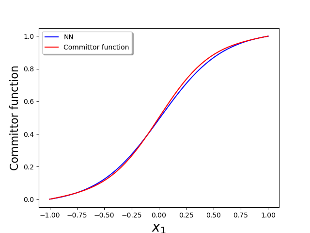
Figure 2: The committor function for the double-well potential along $x_{1}$ dimension when $T=0.5$ for an arbitrarily chosen $(x_{2},\ldots,x_{d})$ with $d=10$.

4.1.1 Comparison with the method of (Khoo et al., 2019)

In this section, we compare the proposed method with the one in (Khoo et al., 2019) in terms of speed, accuracy, and robustness on the double-well potential problem with $T=0.5$. We use the same number of training samples ($1.5\times 10^{5}$) and testing samples ($4.0\times 10^{5}$), NN architectures, and hyperparameters in the implementation of both methods. The numerical tests are carried out on $4$ N$1$ virtual CPUs on the Google Cloud platform with altogether $26$ GB memory and a Tesla K80 GPU. In order to compare penalty coefficients on the same scale, a normalized penalty coefficient $c_{norm}$ is used: it is defined via $c_{norm}=c/\delta$ for the new method with $c$ given in eq:no gradient var and via $c_{norm}=\tilde{c}$ for the old method with $\tilde{c}$ given in weakpenalty.

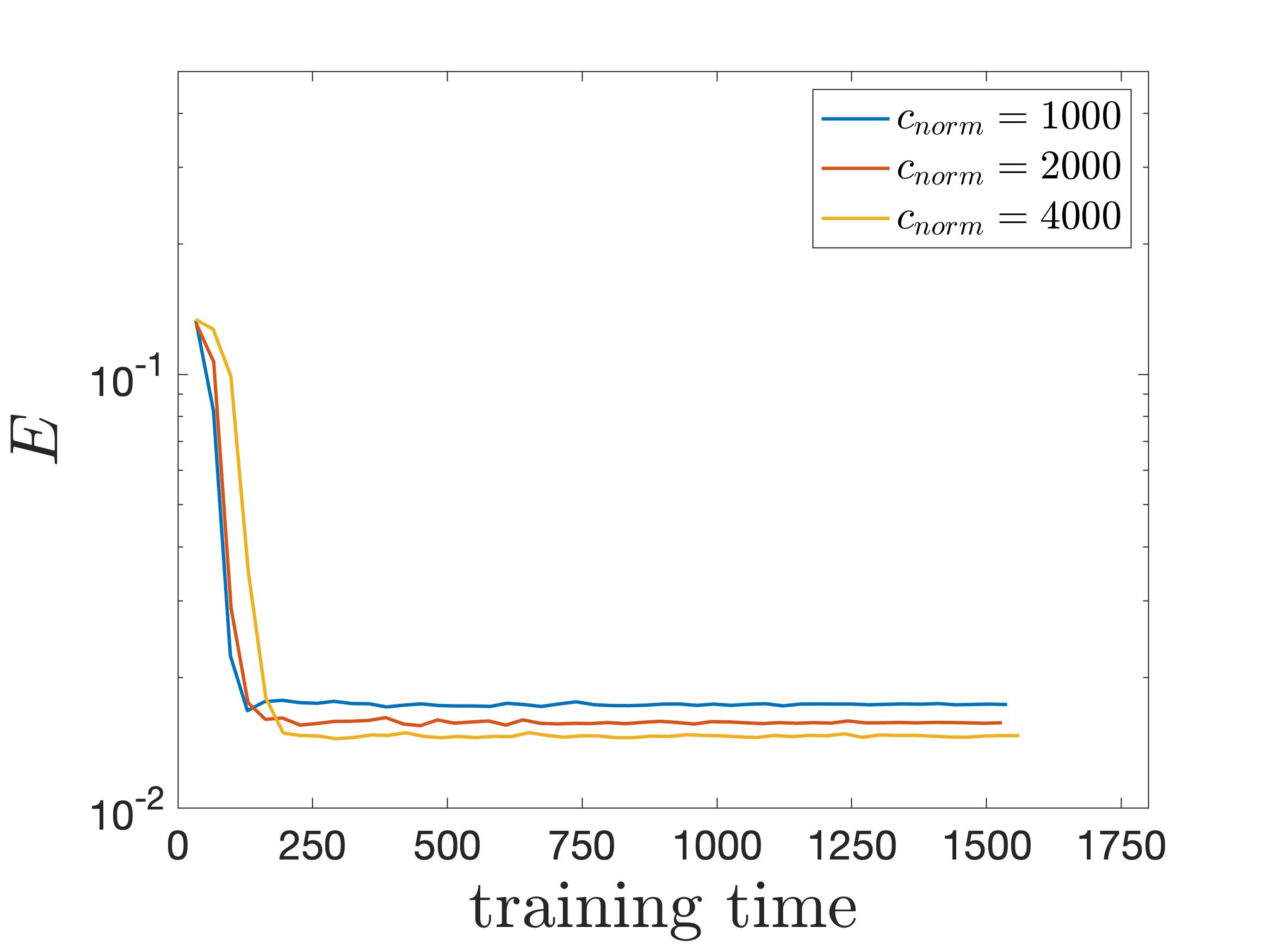
[Training loss of the proposed method]     [Training loss of the method in (Khoo et al., 2019) ]

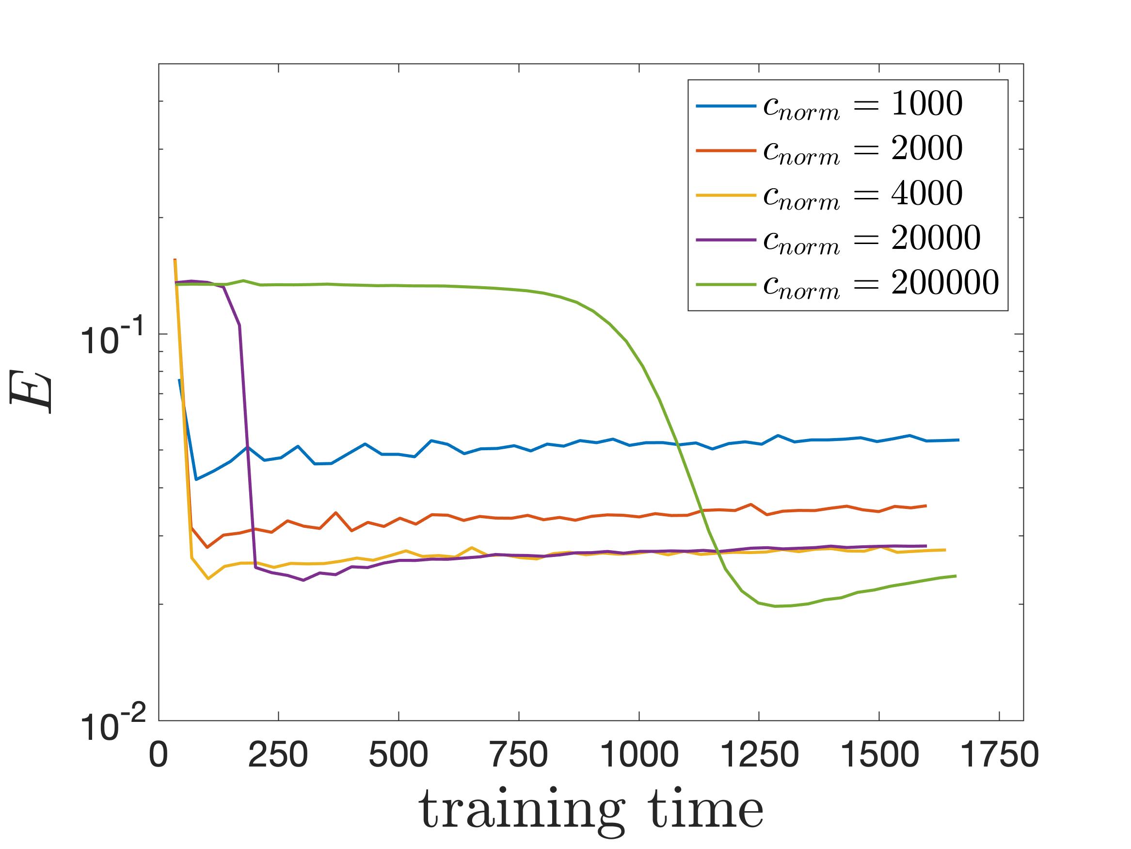
Figure 3: Comparison of the training process of the proposed method and (Khoo et al., 2019)’s method. (a): The training loss versus the training time used for the proposed method. (b): The training loss versus the training time used for the method in (Khoo et al., 2019). We report the error $E$ (defined in eq:error) versus the training time used. Here, $c_{norm}$ stands for the normalized penalty coefficient defined in Section 4.1.1.

Fig. 3 demonstrates a clear difference between the behavior of the two methods during the training. As shown in Fig. 3, when using the method proposed in this paper, the approximate solution converges quickly and the final relative error is rather small, regardless of the choice of penalty coefficients. In contrast, as shown in Fig. 3, when using the method proposed in (Khoo et al., 2019), different penalty coefficients lead to different training behaviors. When the penalty parameter $c_{norm}$ is small, the time used to reach convergence is short but the final relative error is relatively large. When a large penalty parameter is used, the relative error is reduced but it is still higher than the proposed method. Moreover, the time for training to converge is long when using a large penalty parameter. In conclusion, when using the method in (Khoo et al., 2019), the penalty coefficient needs to be carefully tuned in order to have a performance close to the proposed method.

4.2 The rugged-Muller potential

In this example, we consider the committor function corresponding to the following rugged-Muller potential:

$$\aligned V(\mathbf{x})=\tilde{V}(x_{1},x_{2})+\frac{1}{2\sigma^{2}}\sum_{i=3}^{d}x_{i}^{2},$$ (37)

where

$$\tilde{V}(x_{1},x_{2})=\sum_{i=1}^{4}D_{i}e^{a_{i}\left(x_{1}-X_{i}\right)^{2}+b_{i}\left(x_{1}-X_{i}\right)\left(x_{2}-Y_{i}\right)+c_{i}\left(x_{2}-Y_{i}\right)^{2}}+\gamma\sin(2k\pi x_{1})\sin(2k\pi x_{2})$$ (38)

is the $2$-dimensional rugged-Muller potential with the parameters

$$\aligned\left[a_{1},a_{2},a_{3},a_{4}\right]&=[-1,-1,-6.5,0.7],\left[b_{1},b_{2},b_{3},b_{4}\right]=[0,0,11,0.6],\\ \left[c_{1},c_{2},c_{3},c_{4}\right]=[-10,-10,-6.5,0.7],\left[D_{1},D_{2},D_{3},D_{4}\right]=[-200,-100,-170,15],\\ \left[X_{1},X_{2},X_{3},X_{4}\right]=[1,0,-0.5,-1],\left[Y_{1},Y_{2},Y_{3},Y_{4}\right]=[0,0.5,1.5,1],\\ \left[\gamma,k,\sigma,d\right]=[9,5,0.05,10].$$ (39)

The domain of interest $\Omega$ of this example is $[-1.5,1]\times[-0.5,2]\times\mathbb{R}^{d-2}$ and the regions $A$ and $B$ are the following two cylinders:

$$\aligned A&=\left\{\mathbf{x}\in\mathbb{R}^{d}\mid\sqrt{(x_{1}+0.57)^{2}+(x_{2}-1.43)^{2}}\leq 0.3\right\},\\ B=\left\{\mathbf{x}\in\mathbb{R}^{d}\mid\sqrt{(x_{1}-0.56)^{2}+(x_{2}-0.044)^{2}}\leq 0.3\right\}.$$ (40)

In order to compute the error, $q^{*}$ is solved approximately within the $x_{1}x_{2}$-plane. More precisely, we first apply finite element method on uniform grid to committor in $2$ dimensions with the potential $\tilde{V}$, the domain $\tilde{\Omega}=[-1.5,1]\times[-0.5,2]$, and the regions $\tilde{A}$ and $\tilde{B}$ being the projection of the $A$ and $B$ defined in eq:AB onto the $x_{1}x_{2}$-plane. Once the $2$-dimensional committor function $\tilde{q}$ is available, the approximation is $q^{*}(\mathbf{x})=\tilde{q}(x_{1},x_{2})$. The code of the finite element method is provided by the authors of (Lai and Lu, 2018).

As mentioned in Section 2.3, the singularity functions $S_{A}$ and $S_{B}$ should be set as the fundamental solutions of committor when taking $T\rightarrow\infty$. In this case, the limiting committor function as $T\rightarrow\infty$ has the form $q(\mathbf{x})=\tilde{q}(x_{1},x_{2})$ that satisfies a $2$-dimensional Laplace equation, the fundamental solution to which has the form

$$\Phi(x_{1},x_{2})=-\frac{1}{4\pi}\log((x_{1}-a)^{2}+(x_{2}-b)^{2}).$$

Therefore, we set $S_{A}=\log((x_{1}+0.57)^{2}+(x_{2}-1.43)^{2})$ and $S_{B}=\log((x_{1}-0.56)^{2}+(x_{2}-0.044)^{2})$.

Numerical experiments are carried out when $T=22$ and $T=40$. In both situations, $6.0\times 10^{5}$ samples are used in $\Omega\backslash(A\cup B)$. The relative errors are $E=0.024$ when $T=22$, and $E=0.023$ when $T=40$. Table 2 summarizes the numerical error and the parameters used in the experiments.

$(T,\sigma)$	$E$	$\delta$	$c$	No. training samples	Batch size	No. testing samples
(22, 0.05)	0.024	$0.001$	500	$6.0\times 10^{5}$	$5000$	$1.0\times 10^{6}$
(40, 0.05)	0.023	$0.001$	500	$6.0\times 10^{5}$	$5000$	$1.0\times 10^{6}$

Table 2: Results for the rugged-Muller potential problem.

The numerical solution is plotted in Fig. 4, where the exact solutions $q^{*}$ are shown on the left and the committor functions $q_{\theta}$ represented by neural network are plotted on the right. The plots show that the NN approximation shows good agreement with the true solution.

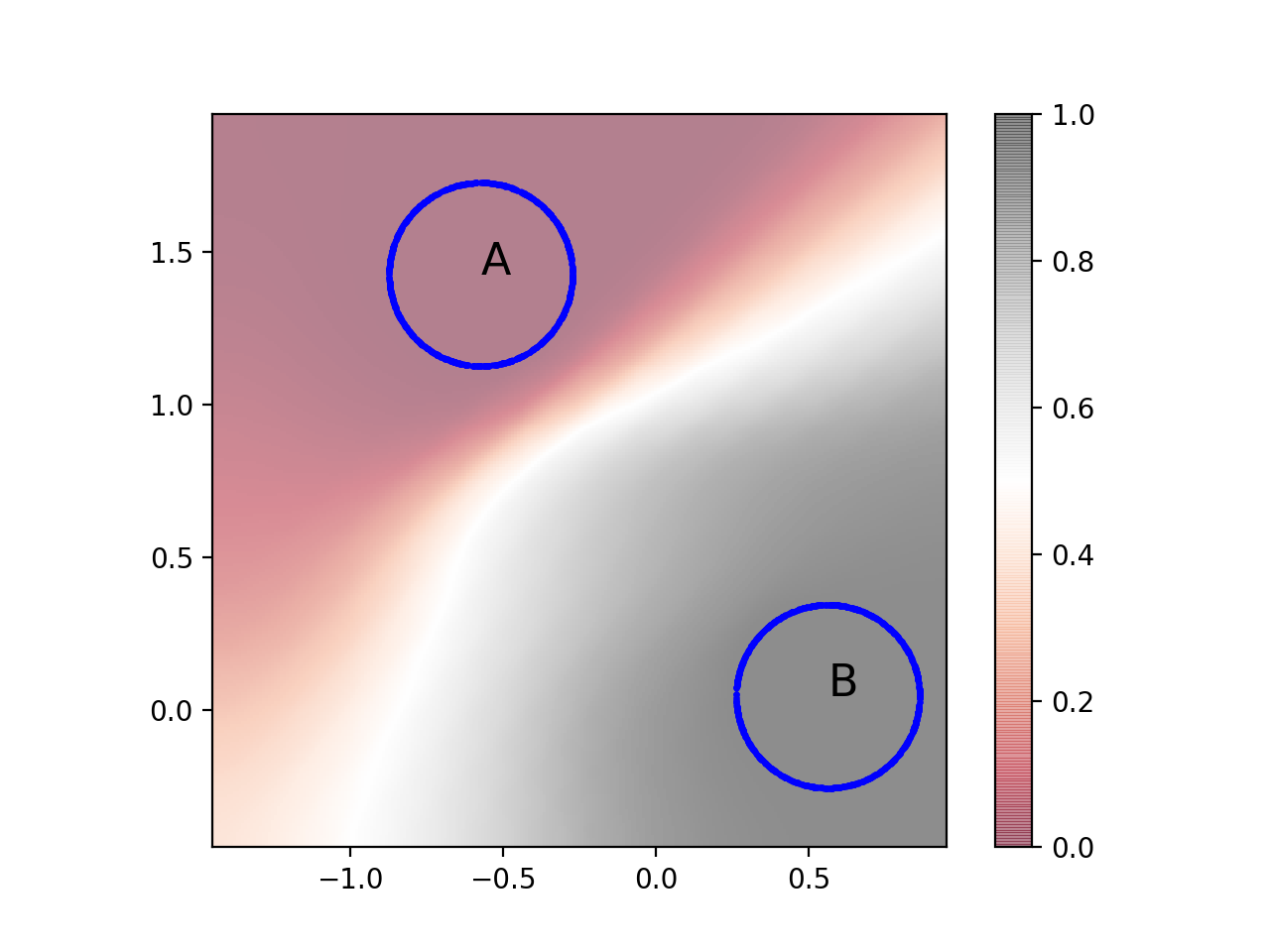
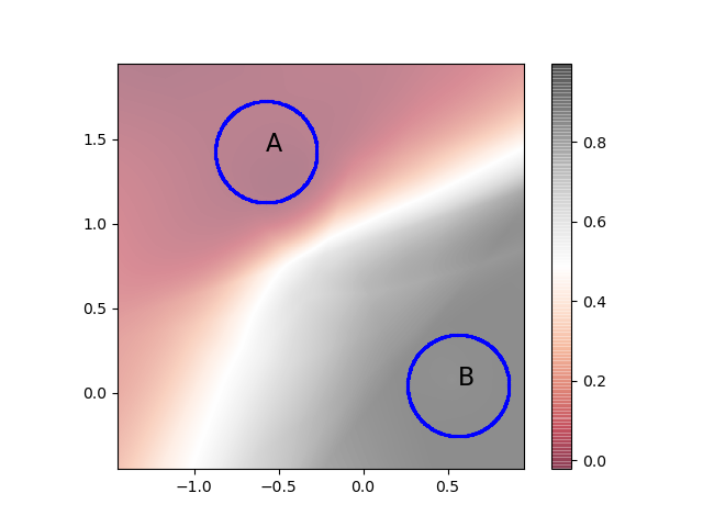
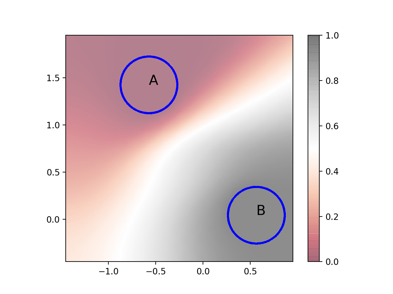
[$T=22$ committor function] [$T=22$ NN approximation] [$T=40$ committor function] [$T=40$ NN approximation]

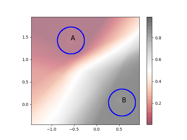
Figure 4: Comparisons between the NN represented committor functions and the ground truths. (a): The ground truth committor function for $T=22$. (b): The NN parameterized committor function for $T=22$. (c): The ground truth committor function for $T=40$. (d): The NN parameterized committor function for $T=40$.

4.3 The Ginzburg-Landau model

The Ginzburg-Landau theory is developed to give a mathematical description of superconductivity (Hoffmann and Tang, 2012). In this example, we discuss a simplified Ginzburg-Landau phase transition model. The Ginzburg-Landau energy in one dimension is defined as:

$$\tilde{V}[u]=\int_{0}^{1}\dfrac{\lambda}{2}u_{x}^{2}+\dfrac{1}{4\lambda}(1-u^{2})^{2}dx,$$ (41)

where $\lambda$ is a small positive parameter and $u$ is a sufficiently smooth function on $[0,1]$ with boundary conditions $u(0)=u(1)=0$.

The high-dimensionality nature of the committor functions is a direct result of the discretization of $u$. With a numerical discretization, $u(x)$ is uniformly discretized by $U=(U_{1},\cdots,U_{d})$ defined on a uniform grid on $[0,1]$ with the boundary conditions $U_{0}=U_{d+1}=0$. Then the continuous Ginzburg-Landau energy is approximated by a discrete one:

$$V(U):=\tilde{V}_{h}[U]=\sum_{i=1}^{d+1}\dfrac{\lambda}{2}\left(\dfrac{U_{i}-U_{i-1}}{h}\right)^{2}+\dfrac{1}{4\lambda}(1-U_{i}^{2})^{2},$$ (42)

where the grid size $h=1/(d+1)$. In this experiment we use $h=1/50$ and the dimension $d=49$. $V(U)$ has two local minima $u_{\pm}(\cdot)$ shown in Fig. 5. The regions A and B are taken as the spheres $\{U:||U-u_{\pm}||\leq r\}$, where $\|\cdot\|$ is the Euclidean norm, and the radius $r$ is chosen to be $3$.

[Local minimizer $u_{-}$] [Local minimizer $u_{+}$]

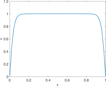
Figure 5: Two local minima of the energy eq:1D discret G-L with $\lambda=0.03$. (a): $u_{-}$, (b): $u_{+}$.

Based on the discretization used, $d=49$. According to Section 2.3, the singularities $S_{A}$ and $S_{B}$ are set to $S_{A}=|U-u_{-}|^{2-d}$, $S_{B}=|U-u_{+}|^{2-d}$. The numerical results are reported for the temperatures $T=30$ and $T=20$. For both cases $2.0\times 10^{5}$ samples are used in $\Omega\backslash(A\cup B)$. In Table 3 we summarize the parameters used in the experiments with $T=30$ and $T=20$.

$T$	$\delta$	$c$	No. training samples	Batch size
20	$0.002$	200	$2.0\times 10^{5}$	$5000$
30	$0.001$	200	$2.0\times 10^{5}$	$5000$

Table 3: Parameters for the Ginzburg-Landau problem.

In this problem, it is intractable to obtain the exact $q^{*}$ due to the high dimensionality and therefore we are not able to estimate the relative error $E$ directly. Instead, we study the region near the $\frac{1}{2}$-isosurface of committor function $q_{\theta}$, which is defined as $\Gamma_{\frac{1}{2},\epsilon}=\{U:|q_{\theta}(U)-\frac{1}{2}|<\epsilon\}$. If $q_{\theta}$ is indeed a satisfactory approximation of $q^{*}$, then for a trajectory given by eq:trajectory starting from an arbitrary point $\mathbf{x}_{0}\in\Gamma_{\frac{1}{2},\epsilon}$, the probability of entering $B$ before $A$ should be close to $\frac{1}{2}$.

More precisely, we first identify $m$ states $\{\tilde{\mathbf{x}}_{j}\}_{j=1}^{m}$ on $\Gamma_{\frac{1}{2},\epsilon}$. From each $\tilde{\mathbf{x}}_{j}$, $N$ trajectories are generated according to eq:trajectory. Let us denote the number of trajectories reaching $B$ before $A$ as $n$. If the NN committor function is accurate, then by the central limit theorem, when $N$ is large, the distribution of $n/N$ should be approximately $\mathcal{N}(\frac{1}{2},(4N)^{-1})$, i.e. the normal distribution with mean $\frac{1}{2}$ and variance $(4N)^{-1}$. In the actual experiment with $\epsilon=0.01$, $m=120$, and $N=100$, the resulting statistics contain $n_{j}/N$ for $j=1,2,\ldots,120$.

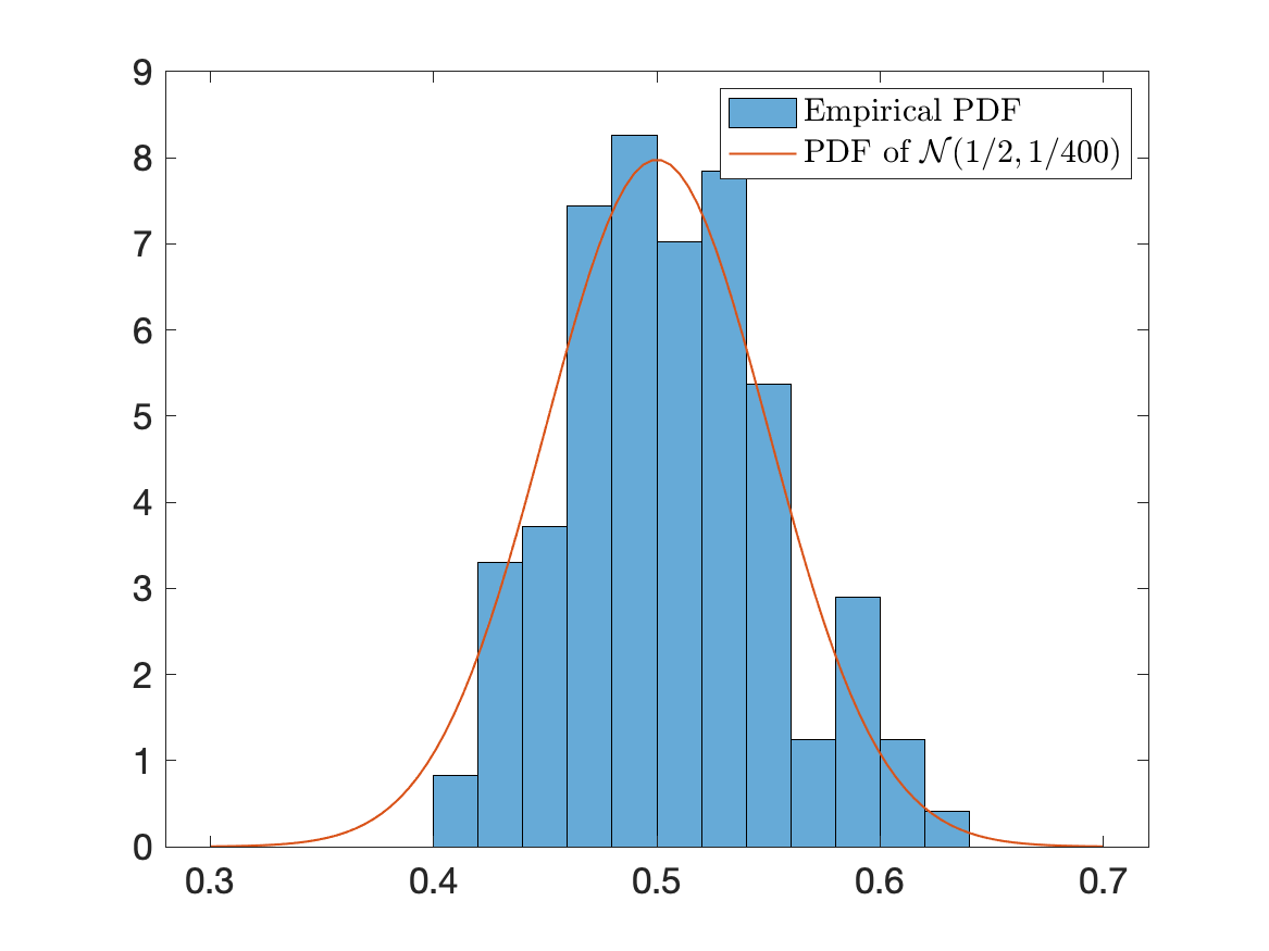
[The empirical PDF versus the PDF of $\mathcal{N}(\frac{1}{2},1/400)$.]     [Q–Q plot of $\{n_{j}/N\}_{j=1}^{120}$ versus $\mathcal{N}(\frac{1}{2},1/400)$.]

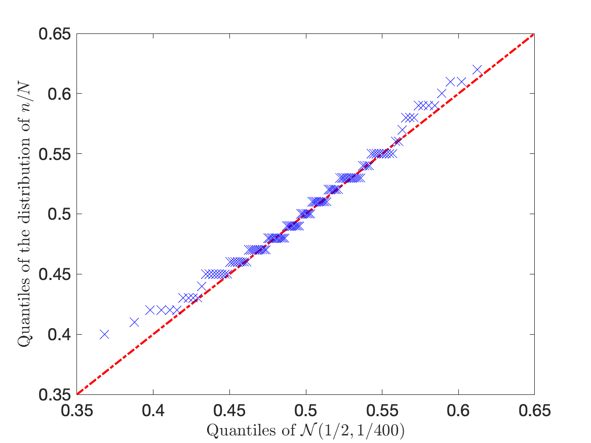
Figure 6: Numerical results of the Ginzburg-Landau model when $T=20$. (a): Empirical probability density function (PDF) of $\{n_{j}/N\}_{j=1}^{120}$ compared with the PDF of $\mathcal{N}(\frac{1}{2},1/400)$. (b): Q–Q (quantile-quantile) plot of $\{n_{j}/N\}_{j=1}^{120}$ compared with the Q-Q plot of $\mathcal{N}(\frac{1}{2},1/400)$.

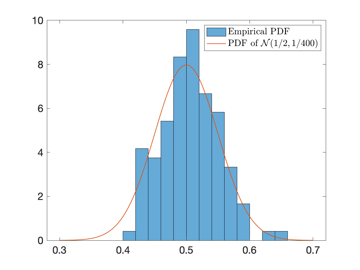
[The empirical PDF versus the PDF of $\mathcal{N}(\frac{1}{2},1/400)$.]     [Q–Q plot of $\{n_{j}/N\}_{j=1}^{120}$ versus $\mathcal{N}(\frac{1}{2},1/400)$]

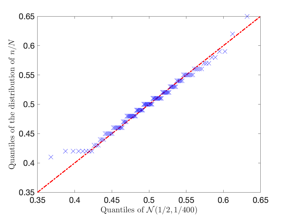
Figure 7: Numerical results of the Ginzburg-Landau model when $T=30$. (a): Empirical PDF of $\{n_{j}/N\}_{j=1}^{120}$ compared with the PDF of $\mathcal{N}(\frac{1}{2},1/400)$. (b): Q–Q (quantile-quantile) plot of $\{n_{j}/N\}_{j=1}^{120}$ versus $\mathcal{N}(\frac{1}{2},1/400)$.

The numerical results we get when $T=20$ and $T=30$ are illustrated in Fig. 6 and Fig. 7, respectively. The histogram of $\{n_{j}/N\}_{j=1}^{120}$ is compared with the normal distribution $\mathcal{N}(\frac{1}{2},1/400)$ on the left, and the Q–Q (quantile-quantile) plot of the distribution of $\{n_{j}/N\}_{j=1}^{120}$ versus $\mathcal{N}(\frac{1}{2},1/400)$ is shown on the right. These figures demonstrate that the distribution of $\{n_{j}/N\}_{j=1}^{120}$ is in good agreement with the normal distribution $\mathcal{N}(\frac{1}{2},1/400)$. As mentioned previously in Section 2.2, we can integrate importance sampling (Li et al., 2019; Rotskoff and Vanden-Eijnden, 2020) when dealing with metastability, especially when the temperature is relatively low. For instance, we can generate the initial state $\mathbf{x}$ in eq:nextstep using importance sampling and then obtain $\mathbf{x}_{\delta}$ via eq:nextstep.

5 Conclusion

In this paper, we improve the method in (Khoo et al., 2019) that solves for the neural network parameterized committor function. In particular, we show that the committor function satisfies an integral equation based on the semigroup of the Fokker-Planck operator. This integral formulation allows us to remove the explicit gradient and handle the boundary conditions naturally. The integrals in the variational form of this new equation can be conveniently approximated via sampling, and the committor function can be solved for using a neural network parameterization and stochastic gradient descent. The resulting algorithm is shown to be faster and less sensitive to the penalty parameter when compared with the approach in (Khoo et al., 2019). The convergence of the training process is guaranteed in the lazy training regime.

This work suggests a few directions of future research. First on the numerical side, the SDE eq:trajectory is currently integrated with the Euler-Maruyama method. It will be useful to explore higher order integration schemes. Our approximation for the stopping time is also rather primitive and it will be beneficial to explore better decision rules. Second, the proposed method can be readily applied to other high-dimensional partial differential equations that possess probabilistic interpretations.

Appendix A Proof of Proposition 2.1

Recall that the Markov semigroup is defined as follows.

Definition 2.

The Markov semigroup $\left(P_{t}\right)_{t\geq 0}$ associated with a Markov process $(\mathbf{x}_{t})_{t\geq 0}$ is defined as

$$P_{t}f(\mathbf{x})=\mathbb{E}^{\mathbf{x}}\left(f\left(\mathbf{x}_{t}\right)\right)=\mathbb{E}\left(f\left(\mathbf{x}_{t}\right)\mid\mathbf{x}_{0}=\mathbf{x}\right),\quad t\geq 0,\quad\mathbf{x}\in\Omega,$$ (43)

where $f:\mathbb{R}^{d}\rightarrow\mathbb{R}$ is bounded continuous.

Recall that $\tau=\tau_{A\cup B}$. While $\tau\wedge\delta$ cannot be directly plugged into Definition 2 since it is a random variable instead of a constant , the operator $P_{\tau\wedge\delta}\equiv P$ can still be defined by eq:beforesplit, and by the strong Markov property of the Langevin process $(\mathbf{x}_{t})_{t\geq 0}$, $(\mathbf{x}_{\tau\wedge\delta})_{\delta\geq 0}$ is also a Markov process, thus $(P_{\tau\wedge\delta})_{\delta\geq 0}$ is a Markov semigroup. Now we proceed to the proof with the help of Dynkin’s formula described in the following theorem:

Theorem A.1.

(Dynkin, 1965)

Consider an Itô diffusion $\{\mathbf{x}_{t}\}_{t\geq 0}$ defined by the following $d$-dimensional stochastic differential equation (SDE)

$$d\mathbf{x}_{t}=b(\mathbf{x}_{t})dt+\sigma(\mathbf{x}_{t})d\mathbf{w}_{t}.$$ (44)

Let $\mathcal{A}$ be the infinitesimal generator of $\{\mathbf{x}_{t}\}_{t\geq 0}$, which is defined by

$$\mathcal{A}f(\mathbf{x})=\lim_{t\rightarrow 0+}\frac{P_{t}f(\mathbf{x})-f(\mathbf{x})}{t},$$ (45)

where $f\in D(\mathcal{A}):=\left\{f\in C_{0}\left(\mathbb{R}^{d}\right)\text{suchthatthelimit\eqref{eq:infi}exists}\right\}$, then for a stopping time $\tau$ such that $\mathbb{E}^{\mathbf{x}}\tau<\infty$,

$$\mathbb{E}^{\mathbf{x}}\left[f\left(\mathbf{x}_{\tau}\right)\right]=f(\mathbf{x})+\mathbb{E}^{\mathbf{x}}\left[\int_{0}^{\tau}\mathcal{A}f\left(\mathbf{x}_{s}\right)\mathrm{d}s\right],$$ (46)

for any $f\in C_{0}^{2}\left(\mathbf{R}^{d}\right)$. Moreover, when $\tau$ is the first exit time for a bounded set, eq:dynkin holds for any $f\in C^{2}\left(\mathbf{R}^{d}\right)$

For any fixed $\delta>0$, $\tau\wedge\delta$ is a stopping time, and is bounded. Although the committor function $q$ may not be compactly supported, we can still use the formula eq:dynkin with the stopping time $\tau\wedge\delta$ replaced by $\tau\wedge\delta\wedge\tau_{B_{r}}$, where $B_{r}$ is the ball with the radius being $r$ and the center being the origin. When $\delta$ is sufficiently small and $r$ sufficiently large, the difference between $P_{\tau\wedge\delta}$ and $P_{\tau\wedge\delta\wedge\tau_{B_{r}}}$ is negligible in practice, as long as $V$ is a confining potential. For this reason, we continue to use the notation $P=P_{\tau\wedge\delta}$ in the problem formulation instead of the more cumbersome $P_{\tau\wedge\delta\wedge\tau_{B_{r}}}$. Therefore for the solution $q$ of the equation committor, we have

$$Pq(\mathbf{x})=q(\mathbf{x})+\mathbb{E}^{\mathbf{x}}\left[\int_{0}^{\tau\wedge\delta}-Lq\left(\mathbf{x}_{s}\right)\mathrm{d}s\right]=q(\mathbf{x}),\quad\forall\mathbf{x}\in\Omega\backslash A\cup B,$$ (47)

as long as we can prove $\mathcal{A}=-L$. In order to show this, we introduce a result in (Kallenberg, 2006).

Theorem A.2.

(Kallenberg, 2006) Assume that $\mathbf{x}_{t}$ satisfies the SDE eq:sde. When $a(\mathbf{x})=\sigma(\mathbf{x})\sigma(\mathbf{x})^{\top}$ and $b$ are bounded and Lipschitz continuous, then the generator $\mathcal{A}$ of the semigroup associated with eq:sde has the following form.

$$\mathcal{A}=\frac{1}{2}\sum_{i,j=1}^{d}a_{ij}(\mathbf{x})\frac{\partial^{2}}{\partial x_{i}\partial x_{j}}+b(\mathbf{x})\cdot\nabla.$$ (48)

Now we are ready to justify eq:replace.

For the Langevin process langevin, the coefficients are $a_{ij}(\mathbf{x},t)=\mathbf{1}_{\{i=j\}}1/\beta$, and $b=\nabla V$, so the conditions in Theorem A.2 on $a$ are naturally satisfied. Since $\nabla V$ is bounded and Lipschitz on $\mathbb{R}^{d}$, the conditions in Theorem A.2 on $b$ are satisfied as well. Thus by Theorem A.2, the generator $\mathcal{A}$ of $(P_{t})_{t\geq 0}$ is

$$\mathcal{A}=\frac{1}{2}\sum_{i,j=1}^{d}\frac{1}{\beta}\mathbf{1}_{\{i=j\}}\frac{\partial^{2}}{\partial x_{i}\partial x_{j}}+\nabla V(\mathbf{x})\cdot\nabla=-L.$$

Plugging this into Dynkin’s formula eq:dynkin yields eq:justifiedreplace, which is what we want to prove.

Appendix B Proof of Proposition 2.1

Consider the stationary Langevin process, i.e. $\{\mathbf{x}_{t}\}_{t\geq 0}$ such that $\mathbf{x}_{0}\sim\rho$ and $\mathbf{x}_{t}$ satisfies langevin. It is known that this process is reversible (see for example (Pavliotis, 2014)). In other words, we have

$$\mathbb{E}_{\mathbf{x}\sim\rho}u(\mathbf{x})v(\mathbf{x}_{\delta})=\mathbb{E}_{\mathbf{x}\sim\rho}u(\mathbf{x}_{\delta})v(\mathbf{x}),$$

for any $u,v\in L_{\rho}^{2}(\Omega\backslash A\cup B)$. Now since the law of the trajectory $\{\mathbf{x}_{\tau\wedge t}\}_{t<\delta}$ is the same as $\{\mathbf{x}_{t}\}_{t<\delta}$ as long as $\delta<\tau$, we have

$$\mathbb{E}_{\mathbf{x}\sim\rho}u(\mathbf{x})v(\mathbf{x}_{\delta})\mathbf{1}_{\{\delta<\tau\}}=\mathbb{E}_{\mathbf{x}\sim\rho}u(\mathbf{x}_{\delta})v(\mathbf{x})\mathbf{1}_{\{\delta<\tau\}},$$

which is exactly $\langle u,P^{i}v\rangle_{\rho}=\langle P^{i}u,v\rangle_{\rho}$.

Appendix C Proof of Proposition 1

eq:pdf can be rewritten as

$$P^{i}f(\mathbf{x})=\int_{\Omega\backslash A\cup B}\!\!\frac{p^{i}(\mathbf{x},\mathbf{y})}{\rho(\mathbf{y})}f(\mathbf{y})\rho(\mathbf{y})d\mathbf{y},$$

and when eq:HS holds, we have

$$\aligned&\iint_{\Omega\backslash A\cup B\times\Omega\backslash A\cup B}\left(\frac{p^{i}(\mathbf{x},\mathbf{y})}{\rho(\mathbf{y})}\right)^{2}\rho(\mathbf{x})\rho(\mathbf{y})d\mathbf{x}d\mathbf{y}\\ =\iint_{\Omega\backslash A\cup B\times\Omega\backslash A\cup B}\!\!\!\!\!\!\!\!\!\!\!\!\!\!\!\!\!\!\!\!\!\!\!\!\!p^{i}(\mathbf{x},\mathbf{y})\frac{\rho(\mathbf{x})p^{i}(\mathbf{x},\mathbf{y})}{\rho(\mathbf{y})}d\mathbf{x}d\mathbf{y}\\ =\iint_{\text{\hbox to10.0pt{$\Omega\backslash A\cup B\times\Omega\backslash A\cup B$\hss\hss}}}p^{i}(\mathbf{x},\mathbf{y})p^{i}(\mathbf{y},\mathbf{x})d\mathbf{x}d\mathbf{y}<\infty,$$

where in the second equality we used the symmetry of $P^{i}$. Thus $P^{i}$ is a Hilbert-Schmidt operator on $L_{\rho}^{2}(\Omega\backslash A\cup B)$ (Dunford and Schwartz, 1965). Thus it is compact, and every point in its spectrum is an eigenvalue. Since $P^{i}$ is contractive, all of its eigenvalues are less or equal than $1$, and it suffices to prove that $1$ is not an eigenvalue for $P^{i}$. If $1$ was an eigenvalue of $P^{i}$, then there exists a nonzero function $f\in L_{\rho}^{2}(\Omega\backslash A\cup B)$ such that $P^{i}f=f$, and by using eq:pdf $n$ times, we get

$$\aligned f(\mathbf{x})&=\int_{\text{\hbox to10.0pt{$\Omega\backslash A\cup B$\hss\hss}}}p^{i}(\mathbf{x},\mathbf{y})f(\mathbf{y})d\mathbf{y}\\ =\iint_{\text{\hbox to10.0pt{$\Omega\backslash A\cup B\times\Omega\backslash A\cup B$\hss\hss}}}p^{i}(\mathbf{x},\mathbf{y})p^{i}(\mathbf{x},\mathbf{z})f(\mathbf{z})d\mathbf{y}d\mathbf{z}\\ =\cdots\\ =\mathbb{E}^{\mathbf{x}}\left(f\left(\mathbf{x}_{n\delta}\right)\mathbf{1}_{\{n\delta<\tau\}}\right),\quad\forall n>0.$$

But the Langevin process langevin is ergodic, and the equilibrium measure $\rho$ is positive, so $\mathbf{1}_{\{n\delta<\tau\}}\rightarrow 0$ almost surely when $n\rightarrow\infty$, resulting in $f=0$, which contradicts with the assumption that $f$ is nonzero. This contradiction shows that $1$ is not an eigenvalue of $P^{i}$ and closes the proof.

References

- Agazzi and Lu (2020) Andrea Agazzi and Jianfeng Lu. Temporal-difference learning with nonlinear function approximation: lazy training and mean field regimes, 2020.
- Chizat et al. (2019) Lenaic Chizat, Edouard Oyallon, and Francis Bach. On lazy training in differentiable programming. In Advances in Neural Information Processing Systems, pages 2937–2947, 2019.
- Coifman et al. (2008) Ronald R Coifman, Ioannis G Kevrekidis, Stéphane Lafon, Mauro Maggioni, and Boaz Nadler. Diffusion maps, reduction coordinates, and low dimensional representation of stochastic systems. Multiscale Modeling & Simulation, 7(2):842–864, 2008.
- Dunford and Schwartz (1965) Nelson Dunford and Jacob T Schwartz. Linear operators. part ii. spectral theory. Bull. Amer. Math. Soc, 2(9904):11348–9, 1965.
- Dynkin (1965) EB Dynkin. Markov processes. vols. i, ii. publishers. New York: Academic Press Inc. Translated with the authorization and assistance of the author by J. Fabius, V. Greenberg, A. Maitra, G. Majone. Die Grundlehren der Mathematischen Wissenschaften, Bände, 121:122, 1965.
- E and Vanden-Eijnden (2006) Weinan E and Eric Vanden-Eijnden. Towards a theory of transition paths. Journal of statistical physics, 123(3):503, 2006.
- E et al. (2005) Weinan E, Weiqing Ren, and Eric Vanden-Eijnden. Finite temperature string method for the study of rare events. J. Phys. Chem. B, 109(14):6688–6693, 2005.
- Hoffmann and Tang (2012) K-H Hoffmann and Qi Tang. Ginzburg-Landau phase transition theory and superconductivity, volume 134. Birkhäuser, 2012.
- Jin et al. (2019) Chi Jin, Praneeth Netrapalli, Rong Ge, Sham M Kakade, and Michael I Jordan. On nonconvex optimization for machine learning: Gradients, stochasticity, and saddle points. arXiv preprint arXiv:1902.04811, 2019.
- Kallenberg (2006) Olav Kallenberg. Foundations of modern probability. Springer Science & Business Media, 2006.
- Khoo et al. (2019) Yuehaw Khoo, Jianfeng Lu, and Lexing Ying. Solving for high-dimensional committor functions using artificial neural networks. Research in the Mathematical Sciences, 6(1):1, 2019.
- Kingma and Ba (2014) Diederik P Kingma and Jimmy Ba. Adam: A method for stochastic optimization. arXiv preprint arXiv:1412.6980, 2014.
- Kloeden and Platen (2013) Peter E Kloeden and Eckhard Platen. Numerical solution of stochastic differential equations, volume 23. Springer Science & Business Media, 2013.
- Kushner and Yin (2003) Harold Kushner and G George Yin. Stochastic approximation and recursive algorithms and applications, volume 35. Springer Science & Business Media, 2003.
- Lai and Lu (2018) Rongjie Lai and Jianfeng Lu. Point cloud discretization of fokker–planck operators for committor functions. Multiscale Modeling & Simulation, 16(2):710–726, 2018.
- Li et al. (2019) Qianxiao Li, Bo Lin, and Weiqing Ren. Computing committor functions for the study of rare events using deep learning. The Journal of Chemical Physics, 151(5):054112, 2019.
- Lu and Nolen (2015) Jianfeng Lu and James Nolen. Reactive trajectories and the transition path process. Probability Theory and Related Fields, 161(1):195–244, 2015.
- Ollivier (2018) Yann Ollivier. Approximate temporal difference learning is a gradient descent for reversible policies. arXiv preprint arXiv:1805.00869, 2018.
- Pavliotis (2014) Grigorios A Pavliotis. Stochastic processes and applications: diffusion processes, the Fokker-Planck and Langevin equations, volume 60. Springer, 2014.
- Rotskoff and Vanden-Eijnden (2020) Grant M. Rotskoff and Eric Vanden-Eijnden. Learning with rare data: Using active importance sampling to optimize objectives dominated by rare events, 2020.
- Vanden-Eijnden and Venturoli (2009) Eric Vanden-Eijnden and Maddalena Venturoli. Revisiting the finite temperature string method for the calculation of reaction tubes and free energies. The Journal of chemical physics, 130(19):05B605, 2009.
- Vanden-Eijnden et al. (2010) Eric Vanden-Eijnden et al. Transition-path theory and path-finding algorithms for the study of rare events. Annual review of physical chemistry, 61:391–420, 2010.