On Duality Gap as a Measure for Monitoring GAN Training

Abstract

Generative adversarial network (GAN) is among the most popular deep learning models for learning complex data distributions. However, training a GAN is known to be a challenging task. This is often attributed to the lack of correlation between the training progress and the trajectory of the generator and discriminator losses and the need for the GAN’s subjective evaluation. A recently proposed measure inspired by game theory - the duality gap, aims to bridge this gap. However, as we demonstrate, the duality gap’s capability remains constrained due to limitations posed by its estimation process. This paper presents a theoretical understanding of this limitation and proposes a more dependable estimation process for the duality gap. At the crux of our approach is the idea that local perturbations can help agents in a zero-sum game escape non-Nash saddle points efficiently. Through exhaustive experimentation across GAN models and datasets, we establish the efficacy of our approach in capturing the GAN training progress with minimal increase to the computational complexity. Further, we show that our estimate, with its ability to identify model convergence/divergence, is a potential performance measure that can be used to tune the hyperparameters of a GAN.

1 Introduction

Generative Adversarial Network(GAN) [1] is probably one of the most important inventions in recent years that is widely popular for modeling data distributions, especially for high dimensional data such as images. A GAN aims to learn a data distribution under adversarial gameplay between two agents - a Discriminator (D) and a Generator (G) parameterized by $\theta_{d}$ and $\theta_{g}$ respectively. The discriminator ($D:X\rightarrow[0,1]$) differentiates between real data samples coming from the distribution to be learned and fake data samples generated by the generator, while the generator ($G:Z\rightarrow X$) aims to fool the discriminator; where $X$ is the data space and $Z$ is the low dimensional latent space. Formally, the GAN objective is defined as

$$\underset{\theta_{g}\in\Theta_{G}}{\min}\ \underset{\theta_{d}\in\Theta_{D}}{\max}\ F(D,G),$$ (1)

$$F(D,G)={\mathop{\mathbb{E}_{\textbf{x}\sim P_{r}}}[\log(D(\textbf{x}))]+\mathop{\mathbb{E}_{\textbf{z}\sim P_{z}}}[\log(1-D(G(\textbf{z})))]}$$ (2)

where $P_{r}$ is the real data distribution and $P_{z}$ is a latent prior. The adversarial game using the above objective has been proven to minimize the Jensen-Shannon (JS) divergence between the true and generated data distributions.

Unlike classical machine learning tasks where the loss functions allow for direct inference on the training progress and a model’s performance, GAN loss functions are non-intuitive and hard to interpret. This is partly due to the stochasticity involved in the training procedure, but mainly because the individual agents’ loss functions also depend on the adversary’s parameters. The alternate optimization changes the individual agents’ loss surface at every iteration, making inference of training progress a challenging task.

Recently, Grnarova et al. suggest the use of duality gap as a measure to monitor the training progress of a GAN. They establish through exhaustive experimentation and theoretical reasoning that the duality gap, being a domain agnostic measure can be used to evaluate GANs over a wide variety of tasks. While the true duality gap is an upper bound on the JS divergence between the real and generated distributions, estimating the true duality gap is an intractable problem. They suggest a gradient descent approach to approximate the duality gap. It is shown that the approximated duality gap can provide insights into the performance a GAN.

While the idea of using the duality gap is promising, the approach to estimating it has an inherent limitation due to the nature of gradient descent and the GAN loss surface. Gradient descent seeks first-order stationary points [2]. In a GAN, a first-order stationary point can be a Nash or non-Nash critical point. We show that the duality gap computed through gradient descent cannot distinguish between these two critical points, which is fundamental to GAN training. Thus, it is not useful for monitoring GAN training.

We propose an effective way to compute the duality gap using locally perturbed gradient descent. The central idea of the approach is to locally perturb a first-order stationary point before applying gradient descent. It can be shown that the local perturbation allows gradient descent to escape from a non-Nash critical point. This effectively differentiates the duality gap computed at Nash and non-Nash critical points.

Overall, we make the following contributions

• We demonstrate a problem with the prevalent approach to estimate the duality gap.

• We propose a theoretically grounded approach to estimate the duality gap through local perturbations that overcomes the limitations of the earlier approach.

• We conduct extensive experiments on a wide variety of GAN models and datasets to demonstrate the domain and model agnostic nature of the proposed measure to monitor the training process.

• We demonstrate that the duality gap can be used as a measure to influence the training process of a GAN, such as tuning hyperparameters. We also show that controllers that maintain the delicate balance between the generator and discriminator updates can be learned using rewards based on duality gap.

2 Related Work

GANs have come a long way since it was proposed by [1]. The various challenges associated with a GAN such as convergence to non-Nash points, lack of diversity in generated samples, diminishing gradients, and enforcing optimal balance between the generator and discriminator have been well-studied. Several loss functions and model architectures have been proposed in this regard [3, 4, 5, 6, 7, 8, 9, 10]. However, despite the numerous advantages, they still fail to provide an insight into the training progress of a GAN, owing to the non-intuitive nature of the associated loss curves. Thus, developing efficient measures for evaluating and monitoring GANs has attracted much interest in recent years [11, 12, 13].

While log-likelihood has been used traditionally to train and evaluate generative models, it is not a suitable measure for a likelihood-free model like GAN. Further, estimating likelihood is intractable and subject to error in higher dimensions [14]. Among the popular metrics to assess GANs are - Inception Score (IS)[15] and Frechet Inception Distance (FID) [8]. IS evaluates a batch of generated images based on the ability of a pre-trained inception network to accurately classify them among known Image-Net classes - while the entropy of the predicted labels of the generated distribution captures the diversity, quality is implicitly captured by the inception score as the proximity of the generated samples to the real samples. However, as IS does not statistically compare the real and generated distributions, it is not sensitive to mode collapse. FID overcomes this weakness of IS, but it assumes the embedding from the inception network to be Gaussian, which is unrealistic. Both FID and IS are restricted only to images. [16] propose precision and recall to capture the fidelity and diversity aspects of generative models. Precision quantifies the quality of the generated samples, and recall estimates the proportion of the real distribution covered by the generated distribution. However, they assume that the embedding space is uniformly dense and rely on the sensitive $k$-means clustering to determine the support set. [17] improve precision and recall by estimating the probability density using $k$-nearest neighbors. However, the improved precision and recall are sensitive to outliers. [18, 19] propose Density and Coverage to reduce the overestimation of manifold due to outliers.

Apart from the requirement of labeled data (pre-trained networks), the above mentioned measures are domain-dependent, constraining their application to image datasets. Further, the best values of these measures are subjective to the real data, and hence there is no generic bound on these metrics to judge that the training has converged. There is a need for an intuitive metric that is domain agnostic, computationally feasible, and gives insight into the GAN training. [20] propose such an efficient metric - the Duality Gap to monitor the training progress of GANs. Unlike other metrics, duality gap is neither restricted to a specific data distribution nor requires a pre-trained neural network and is lower bounded by JS divergence between real and generated distributions. Our work is a study of the estimation process of the duality gap, aiming to improve its efficiency as a performance monitoring tool for GANs.

3 Methodology

3.1 Preliminaries

Game Theoretic and Optimization Perspectives : In the standard formulation of a GAN (equation 1), the equilibrium for the adversarial game play between the generator and the discriminator is the Nash equilibrium [1]. At such an equilibrium, the divergence between the real and generated distribution is minimum. Formally, a configuration or strategy $(\theta_{g}^{*},\theta_{d}^{*})$ is said to be a pure Nash equilibrium, if:

$$F(\theta_{g}^{*},\theta_{d})\leqslant F(\theta_{g}^{*},\theta_{d}^{*})\leqslant F(\theta_{g},\theta_{d}^{*})\ \forall\ \theta_{g},\theta_{d}$$ (3)

Equivalently,

$$\underset{\theta_{g}\in\Theta_{G}}{\min}F(\theta_{g},\theta_{d}^{*})\ =\ \underset{\theta_{d}\in\Theta_{D}}{\max}\ F(\theta_{g}^{*},\theta_{d})=F(\theta_{g}^{*},\theta_{d}^{*})$$ (4)

However, finding the global Nash equilibrium is hard because the loss surface for the GAN optimization is not convex-concave [21]. Typically, a Local Nash Equilibrium (LNE) is what we expect to attain. Formally, a configuration $(\theta_{g}^{*},\theta_{d}^{*})$ is said to be a pure LNE, if $\exists\delta>0\ \mbox{such that}\ \forall\ \theta_{g},\theta_{d}\ \mbox{ with }\ \|\theta_{g}-\theta_{g}^{*}\|\ <\delta\ \mbox{and}\ \|\theta_{d}-\theta_{d}^{*}\|<\delta$,

$$F(\theta_{g}^{*},\theta_{d})\leqslant F(\theta_{g}^{*},\theta_{d}^{*})\leqslant F(\theta_{g},\theta_{d}^{*})$$ (5)

It is known that the GAN loss surface has abundant saddle points [7, 22]. Thus we must understand the characteristics of the LNE, a saddle point that we seek. As neural networks parameterize our models, we use gradient-based alternate optimization to seek the LNE $(\theta_{g}^{*},\theta_{d}^{*})$, which is a local maximum w.r.t the maximizing agent (discriminator) and a local minimum w.r.t the minimizing agent (generator). Formally, the local Nash Equilibrium $(\theta_{g}^{*},\theta_{d}^{*})$ satisfies

$$\nabla_{\theta_{g}}F(\theta_{g}^{*},\theta_{d}^{*})=0\text{ and }\nabla_{\theta_{d}}F(\theta_{g}^{*},\theta_{d}^{*})=0$$ (6)

$$\frac{\partial^{2}F(\theta_{g}^{*},\theta_{d}^{*})}{\partial{\theta_{g}}^{2}}\succ 0\text{ and }\frac{\partial^{2}F(\theta_{g}^{*},\theta_{d}^{*})}{\partial{\theta_{d}}^{2}}\prec 0,$$ (7)

We expect the gradient dynamics associated with the alternate optimization to enforce convergence to a local Nash Equilibrium. However, in practice, there are a plethora of non-Nash critical points that are attractors (satisfy only equation 6) under the gradient dynamics [7], thus making the training of GANs unstable and cumbersome.

3.2 Duality Gap for Monitoring GAN Training

A good measure for monitoring GAN training should be domain agnostic and enable easy inference of the training progress. Duality Gap [20] is a recently proposed measure motivated by principles of game theory.

Definition 1.

(Duality Gap) Let $\Theta_{D}$ and $\Theta_{G}$ denote the parameter spaces of the discriminator and the generator respectively. Then for a pure strategy $(\theta_{g},\theta_{d})$ such that $\theta_{g}\in\Theta_{G}$ and $\theta_{d}\in\Theta_{D}$, the Duality Gap, is defined as

$$DG(\theta_{g},\theta_{d})=\underset{\theta_{d}^{{}^{\prime}}\in\Theta_{D}}{\max}\ F(\theta_{g},\theta_{d}^{{}^{\prime}})\ -\ \underset{\theta_{g}^{{}^{\prime}}\in\Theta_{G}}{\min}F(\theta_{g}^{{}^{\prime}},\theta_{d})$$ (8)

Intuitively, the duality gap measures the maximum payoff the agents can obtain by deviating from the current strategy. At Nash Equilibrium, as no agent can unilaterally increase their payoff, the duality gap is zero. This is implied by equation (4). Further, the duality gap is always non-negative. Grnarova et al. show that the duality gap is lower bounded by the Jensen-Shannon divergence between the true and generated data distributions. While the duality gap seems to be a useful performance measure for GANs, computing the exact duality gap at any point is an NP-hard problem as it involves finding the extrema of non-convex functions [23, 20].

3.2.1 Duality Gap Estimation

The duality gap is estimated through an iterative gradient based optimization [20]. An auxiliary generator and discriminator are initialized to the current values $(\theta_{g}^{t},\theta_{d}^{t})$ of their GAN counterparts at iteration $t$. The auxiliary discriminator is optimised for a fixed number of iterations to obtain the worst case discriminator ($\theta_{d}^{w}$) to compute $M_{1}=F(\theta_{g}^{t},\theta_{d}^{w})$. Analogously, the auxiliary generator is optimised to obtain the worst case generator ($\theta_{g}^{w}$) to compute $M_{2}=F(\theta_{g}^{w},\theta_{d}^{t})$. The difference $M_{1}-M_{2}$ is the estimated duality gap at the iteration $t$.

3.2.2 The Challenge

This estimation process seems very intuitive from the game theory perspective as it imitates the individual players’ efforts to unilaterally increase their payoffs by deviating from their current strategy. However, it limits the ability of the estimated duality gap as a performance metric to distinguish clearly between stable mode collapse, divergence and convergence encountered during GAN training. This is because, the gradient based optimizations for computing $M_{1}$ and $M_{2}$ seek first order stationary points i.e. points where the gradients of the objective function w.r.t to the optimizing agent is zero. As Nash and non-Nash critical points are both first order stationary points [24], the duality gap estimated would be very close to zero. This is evident from the updates for estimating the worst case generator and discriminator. At the critical point $(\tilde{\theta}_{g},\tilde{\theta}_{d})$, $\nabla_{\theta_{g}}F(\tilde{\theta}_{g},\tilde{\theta}_{d})\mbox{=}0$ and $\nabla_{\theta_{d}}F(\tilde{\theta}_{g},\tilde{\theta}_{d})\mbox{=}0$ due to the first-order stationarity property. Thus it acts as an attractor in the gradient optimization for estimating the worst case generator ($\theta_{g}^{w}$) and discriminator ($\theta_{d}^{w}$). Thus $({\theta_{g}^{w}},{\theta_{d}^{w}})\mbox{=}(\tilde{\theta}_{g},\tilde{\theta}_{d})$, which in turn results in $M_{1}\mbox{=}M_{2}$ and hence $DG(\tilde{\theta}_{g},\tilde{\theta}_{d})\mbox{=}0$. Thereby making it hard to differentiate between Nash and non-Nash critical points. However, at a non-Nash critical point, at least one of the agents can increase the payoff by deviating from the current strategy. It is the inherent limitation of the estimation process that the auxiliary models are unable to escape the non-Nash critical points [7].

To circumvent the optimization for estimating the worst discriminator and generator, [20] suggests estimating the approximate duality gap by choosing the most adversarial discriminator and generator from the saved set of snapshots of generator and discriminator parameters at different training time instants. This approximation requires the book-keeping of the discriminator and generator snapshots at different timestamps throughout the training. It is non-intuitive as it is uncertain if the worst generator/discriminator for a particular configuration would have been encountered previously during the GAN training.

3.3 Perturbed Duality Gap

We propose an effective way to compute the duality gap accurately using locally perturbed gradient descent. The method introduces perturbations to the worst-case agent’s initial point in its local neighborhood before applying gradient descent. Algorithm 1 summarizes the modified estimation process. The auxiliary generator and discriminators’ parameters are initialized to the current iterate values, $\theta_{g}^{t}$ and $\theta_{d}^{t}$, respectively. The initialization is perturbed by adding noise sampled uniformly from a ball of radius $\sigma$. Optimization is performed on the perturbed initialization to estimate the worst-case generator ($\theta_{g}^{w}$) and discriminator ($\theta_{d}^{w}$). The success of the method relies on the perturbation that is applied to the initialization. We discuss the intuition of the local perturbation in the next subsection and present a way to limit the radius of the perturbation ball in the experiments.

Input: Current iterate values of G and D - $\theta_{g}^{t}$, $\theta_{d}^{t}$

$\theta_{d}^{a}\longleftarrow\ \theta_{d}^{t}+\delta$

$\theta_{g}^{a}\longleftarrow\ \theta_{g}^{t}+\delta$

where $\delta\sim U([-\sigma,\sigma])$

for i in Iterations do

      $\theta_{d}^{a}\longleftarrow\ \theta_{d}^{a}+\eta\nabla_{\theta_{d}^{a}}F(\theta_{g}^{t},\theta_{d}^{a})$

       $\theta_{g}^{a}\longleftarrow\ \theta_{g}^{a}-\eta\nabla_{\theta_{g}^{a}}F(\theta_{g}^{a},\theta_{d}^{t})$

end for

$(\theta_{g}^{w},\theta_{d}^{w})$ are the converged worst cases

$M_{1}=F(\theta_{g}^{t},\theta_{d}^{w})$

$M_{2}=F(\theta_{g}^{w},\theta_{d}^{t})$

return $DG(\theta_{g}^{t},\theta_{d}^{t})$ = $M_{1}-M_{2}$

Algorithm 1 Perturbed Duality Gap DG ($\theta_{g}^{t}$, $\theta_{d}^{t}$)

3.3.1 Intuitive and Theoretical Understanding

The intuitive and theoretical understanding of the proposed method is inspired from the work on escaping saddle points during gradient descent [25]. Let $(\theta_{g},\theta_{d})$ be a configuration at which we would like to compute the duality gap. Without loss of generality, let us consider the optimization to compute $M_{2}$. Let $(\theta_{g}^{a},\theta_{d})$ be the perturbed initial point and $(\theta_{g}^{w},\theta_{d})$ be the estimated worst case configuration. We can visualize $(\theta_{g}^{a},\theta_{d})$ as sampled from a perturbation ball ($B$) centered at $(\theta_{g},\theta_{d})$ with radius $\sigma$. The three possible situations at $(\theta_{g},\theta_{d})$ are (1) Gradients are sufficiently large; (2) Gradients are close to zero, but hessian is not positive semidefinite ($(\theta_{g},\theta_{d})$ is a first order stationary point); (3) Gradients are close to zero and hessian is positive semidefinite ($(\theta_{g},\theta_{d})$ is a second order stationary point). In the first case, as $F(.)$ is smooth, classical gradient descent will reduce the function value.

The second and third cases are of specific interest because they are usually encountered during GAN training as convergence to non-Nash and Nash critical points respectively. If $(\theta_{g},\theta_{d})$ is a non-Nash critical point (the second case), we would like gradient descent starting from $(\theta_{g}^{a},\theta_{d})$ (the perturbed initialization) to escape the saddle point thereby minimising the function value. This is guaranteed by the theoretical results in [25] (Lemma 10). The intuition behind the theory revolves around understanding the geometry of the perturbation ball ($B$) around the saddle point. Let us denote by $B_{S}$ - the stuck region inside $B$ from which gradient descent would be unable to escape the saddle point. Jin et al. show that this region’s volume is minimal compared to the perturbation ball’s overall volume. Thus after adding the perturbation to $\theta_{g}$, the point $\theta_{g}^{a}$ has a small chance of falling in $B_{S}$ and hence will escape from the saddle point efficiently. The same reasoning can be analogously applied to the discriminator parameters while computing $M_{1}$. The direct inference from the above is that the perturbed duality gap estimate would be non-zero at non-Nash critical points and close to zero in the vicinity of Nash critical points, thus enabling better differentiation between convergence/non-convergence scenarios.

The local perturbations to the initial point might not be very intuitive from the game theory perspective as it does not precisely measure the effect of deviating from the current strategy. However, the estimation process is consistent because the perturbations are local (reachable) and only for the agent that is to be optimized. Hence should not significantly affect the optima to be attained as the loss surface remains unchanged. Incorporating this subtle modification will enable us to differentiate between convergence to Nash and non-Nash critical points.

We know that an LNE is a locally stable and attracting critical point for both the agents. Thus, despite the local perturbations, during convergence to a local Nash Equilibrium $(\theta_{g}^{*},\theta_{d}^{*})$, the worst case discriminator while computing $M_{1}$ and the worst case generator while computing $M_{2}$ would ideally correspond to $(\theta_{d}^{*}$ and $\theta_{g}^{*})$ respectively. Thus the duality gap would still be close to zero. When the agents converge to a non-Nash critical point $(\theta_{g}^{{}^{\prime}},\theta_{d}^{{}^{\prime}})$, the original estimation process for $M_{1}$ and $M_{2}$ would result in the worst case discriminator and generator restricted to $(\theta_{d}^{{}^{\prime}}$ and $\theta_{g}^{{}^{\prime}})$ due to the lack of gradients in the vicinity of the saddle point. However, the introduction of local perturbations displaces the agent from the saddle point and provides the additional momentum required to escape the non Nash critical point, preventing the estimated duality gap from saturating to zero.

4 Experiments and Results

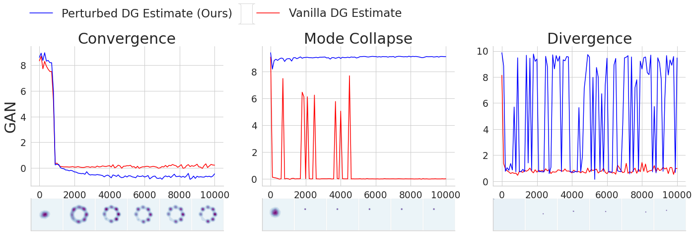
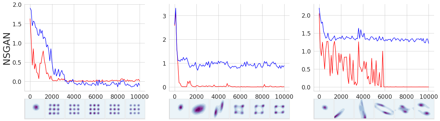
Figure 1: Perturbed and Vanilla DG estimate throughout the training progress of classic GAN (top row) and NSGAN (bottom row) on the RING and GRID datasets respectively for the scenarios - convergence (left column), mode collapse (middle column), and divergence (right column). For each sub-graph, X-axis corresponds to the number of iterations, and Y-axis corresponds to the estimated duality gap.

We design experiments to investigate the commonly encountered failure cases during GAN training from the perspective of the duality gap (DG). We empirically show that the proposed method, which we refer to as perturbed DG estimate, is better equipped to monitor the GAN training than the estimate of Grnarova et al., which we refer to as vanilla DG estimate. Our objective is to only provide a rigorous comparison between the vanilla and perturbed DG estimate, for monitoring GAN training and is not on analyzing different GAN variants or datasets. The source code and other experimental details are publicly available . We illustrate the hypothesized behaviour of the DG estimates near Nash and non-Nash critical points using a toy function in the supplementary material. We begin the discussion with the mixture of Gaussians.

4.1 Mixture of Gaussians

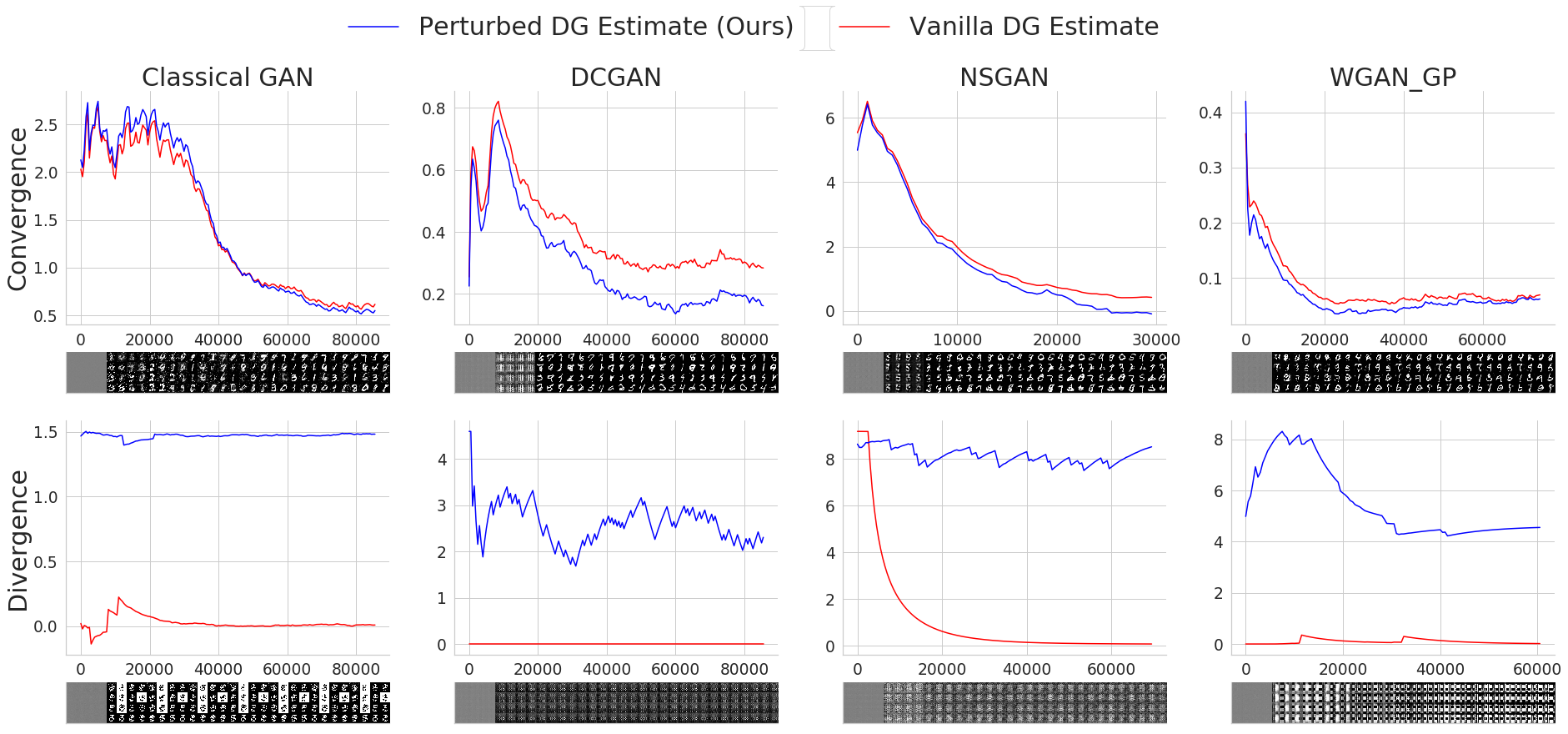
(a) Classic GAN, DCGAN, NSGAN and WGAN-GP on MNIST dataset

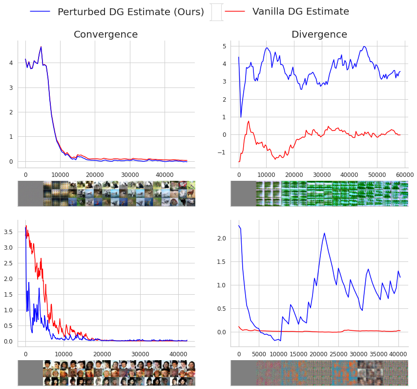
(b) WGAN-GP on CIFAR-10 and CELEBA datasets

Figure 2: Comparison of perturbed and vanilla DG estimate throughout the training progress of various GANs on image datasets across convergence and divergence settings.

We use three toy Gaussian mixture datasets (RING, GRID, and SPIRAL) to monitor the GAN training process using the estimated duality gap. For each of these datasets, we train a classical GAN and its non-saturating (NSGAN) counterpart. We simulate convergence, mode collapse, and divergence scenarios by varying the learning rate and update sequence of generator and discriminator. We analyze the results for training the classical GAN and NSGAN on the RING and GRID datasets. Similar patterns observed for the other datasets are discussed in the supplementary material.

Figure 1 demonstrates the sensitivity of the perturbed and vanilla duality gap estimates during convergence, mode collapse, and divergence throughout the training progress of a classic GAN and NSGAN on the RING and GRID datasets respectively. We observe that the behavior of perturbed and vanilla DG estimates is alike during convergence as both saturate close to zero as expected. The duality gap estimate being marginally negative at times despite the true duality gap being lower bounded by the JS divergence can be understood as a limitation posed by the approximation as discussed in [20], and does not to a large extent affect its ability to capture the training progress. We observed that the Vanilla DG estimate saturates to values very close to zero during mode collapse and divergence while perturbed DG saturates (or oscillates) to non-zero positive values as expected. Thus, we verify that our approach can escape non-Nash saddle points and, therefore, can better track the training progress of the GANs.

4.2 Image Datasets

Having established the efficacy of our approach on synthetic datasets, we now focus on confirming the generality of perturbed DG across GAN architectures in learning higher dimensional data distributions. To this end, we train a classical GAN, DCGAN, DCGAN+NS (NSGAN), WGAN-GP over image datasets - MNIST, Fashion-MNIST, CIFAR-10, and CelebA [26, 27, 28, 29]. To get an unbiased estimate of the DG, we split the datasets into a disjoint train, validation, and test sets to train the GAN, find the worst-case generator/discriminator, and evaluate the objective function w.r.t the worst-case agents respectively. We use classic GAN objective as a reference as suggested by [20] and train worst-case agents for 400 iterations using the optimizer of their GAN counterparts for estimating the duality gap. We simulate convergence and non-convergence scenarios by varying the learning rates.

4.2.1 MNIST and Fashion MNIST

Figure 2(a) validates the generality of perturbed DG estimates across GAN architectures for the MNIST dataset. As expected, we observe that both vanilla and perturbed DG estimates saturate close to zero during convergence irrespective of the GAN architecture. However, the vanilla DG estimate saturates close to zero even when the GAN diverges. On the contrary, the perturbed DG estimate shows a higher sensitivity to the divergence setting by saturating to a non-zero positive value. We repeat this experiment on the Fashion MNIST dataset and illustrate the results in the supplementary material. In addition to convergence and divergence settings, the perturbed DG estimate is also sensitive to mode collapse even for complex data distributions as suggested by the results presented in the supplementary material.

4.2.2 CIFAR-10 and CelebA

We investigate the generality of perturbed DG for monitoring the GAN training progress on complex image distributions like CIFAR-10 and CelebA. We choose WGAN-GP, a widely accepted GAN model for learning high dimensional data distributions, for this experiment. Results of this experiment (Figure 2(b)) show that the perturbed DG estimate can clearly differentiate between convergence and divergence, validating the hypothesis that the choice of the data distribution and GAN architectures do not constrain the sensitivity of the perturbed DG estimate towards convergence and (or) non-convergence.

4.3 Influencing GAN Training using perturbed DG

A generic framework for tuning the hyperparameters of a GAN with minimal human intervention has been an open problem in the community due to a lack of domain agnostic measures capable of accurately quantifying a GAN’s performance. The convergence of a GAN largely depends on preserving the delicate balance between the generator and discriminator [10] that is governed by the tuning of hyperparameters. We show empirically that perturbed DG can be used to fine tune these hyperparameters. Further, perturbed DG can facilitate learning of meta-models that can automatically drive a GAN to convergence.

4.3.1 Hyperparameter Search

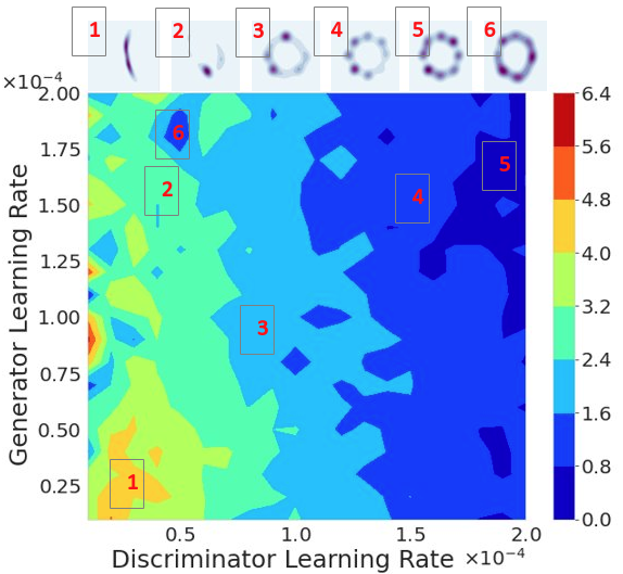
(a)

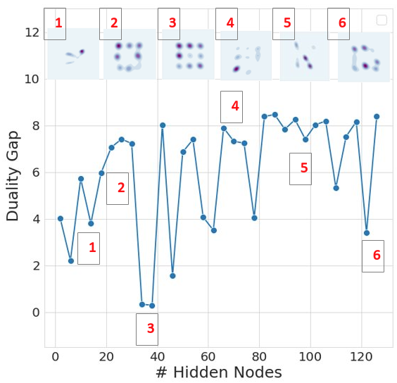
(b)

Figure 3: [Best viewed in color] Perturbed DG trend across: (a) Learning rates (b) Model Capacity

We focus on tuning the learning rates and model capacity. We perform a grid search on these hyperparameters and compute the perturbed DG estimate at every choice to identify the optima. The learning rates of both the generator and the discriminator impact each other. Thus we search over the 2D space defined by both the parameters. Figure 3(a) depicts the contour plot for the perturbed DG estimate over this space for a classic GAN trained on the RING dataset. The optimal range of learning rates for the generator and the discriminator can be easily identified as the region where perturbed DG approaches zero. The optimal learning rates, as suggested by the perturbed DG estimate, are further verified by visualizing the similarity of the generated and true data distribution in these regions. As for model capacity, we search over the space defined by the number of hidden nodes in each layer of the models - we use the same number of layers and hidden nodes for both the generator and the discriminator. This is visualized in Figure 3(b) for a classical GAN trained on the GRID dataset. We observe an optimum capacity for the models at which the game is balanced, and the perturbed DG estimate can identify it as the region where the duality gap is close to zero.

4.3.2 Dynamic Scheduling

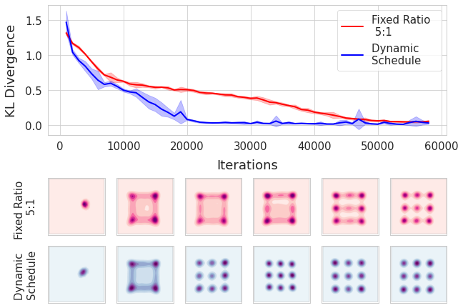
(a) GRID Dataset

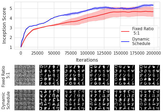
(b) MNIST Dataset

Figure 4: [Best viewed in color] Dynamic scheduling using perturbed DG based controller leads to faster convergence.

Another dimension governing the balance between the generator and discriminator is the schedule that drives the underlying alternate iterative optimization. [30] shows that a dynamic schedule that considers the current state and the history of the optimization procedure over following a fixed schedule can lead to better convergence for GANs. They use a controller network, learned using a policy gradient method to maximize the expected reward defined in terms of the final performance of the GAN, to generate a dynamic schedule. However, they quantify the GAN performance using the Inception Score, limiting its applicability to only images. We extend their approach by superseding the inception score with perturbed DG as the reward for training the controller. We define the input space of the controller as a 4-tuple - (a) the log-ratio of the magnitude of the gradients of the generator and discriminator, an exponential moving average of - (b) generator’s loss, (c) discriminator’s loss, and (d) perturbed DG. Such a state representation is independent of the GAN architecture and captures sufficient information needed to infer the balance between the agents. As there is an inverse relation between perturbed DG ($DG$) and convergence of a GAN, we specify the reward as $\frac{\alpha}{DG+\epsilon}$, where $\alpha$ is a reward constant and $\epsilon$ is added for numerical stability. The domain agnostic nature of the duality gap enables learning dynamic schedules for GANs irrespective of the data distribution and also facilitates learning a domain agnostic controller that is generalizable across GAN architectures and domains. We verify this hypothesis by training a controller using perturbed DG to enforce convergence of a WGAN-GP on the 2D RING dataset. We then use this trained controller to drive the training of a WGAN-GP on the 2D GRID dataset and a convolutional WGAN-GP on the MNIST dataset.

The implementation details regarding the training procedure of the controller are provided in the supplementary material. Figure 4 depicts the average performance of the dynamic schedule against the suggested discriminator-generator update ratio of 5:1 for WGAN-GP, in terms of domain-specific evaluation criteria for each the above settings - KL divergence for 2D GRID and Inception Score for MNIST. We observe that the dynamic schedule leads to faster and better convergence for each of the above settings. The KL divergence between the real and generated distributions quickly saturates close to zero for the 2D GRID and the higher inception scores for MNIST are obtained when using the dynamic schedule predicted by the controller network. Thus, while the balance enforced by the controller helps transcend manual tuning of the schedule, its generalizability, owing to the domain agnostic nature of perturbed DG, outweighs the effort invested in its training process.

4.4 Ablation Studies

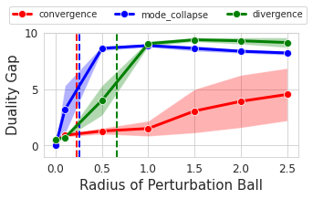
(a)

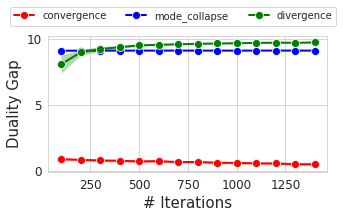
(b)

Figure 5: Ablation Studies: (a) Perturbed DG estimate for varying radii of the perturbation ball. (b) Perturbed DG estimates w.r.t training iterations of the auxiliary GAN.

4.4.1 Perturbation Ball Radius

An unknown in the proposed perturbed DG estimation process is $\sigma$, the radius of the perturbation ball. We investigate the effect of $\sigma$ on DG estimate for three settings, namely convergence, mode collapse, and divergence. We train a classic GAN on the RING dataset for conducting this study. We estimate the saturated DG value at the end of 20,000 iterations for each setting and monitor the impact of $\sigma$ on the perturbed DG values across 50 trials. We observe from figure 5(a) that the DG steadily increases with $\sigma$ during the convergence setting. However, there is a steeper increase in DG values for mode collapse and divergence setting saturating to a positive value. The size of the stuck region in the perturbation ball could explain this behavior. During convergence, the model converges to a Nash point enclosed in a larger stuck region within the perturbation ball due to which sufficiently large $\sigma$ is required to push the model off the stuck region. On the contrary, during non-convergence, the model converges to a non-Nash critical point enclosed in a comparatively thin stuck region. Therefore a small increase in $\sigma$ is sufficient to push the model off the stuck region.

We also notice an increasing trend in the DG variance for the convergence setting across trials compared to other scenarios. This behavior is explained by observing that the perturbations across the trials are stochastic, and for some trials, it may be sufficient for the model to escape the stuck region compared to other trials. However, even a small perturbation is sufficient for the model to escape the stuck region for mode collapse and divergence settings, further indicating that the stuck region’s volume is small for these non-Nash critical points arrived during GAN training.

We now draw the attention towards the approximation of $\sigma$ by the standard deviation of the model’s weights. In figure 5(a), red, blue, and green vertical lines correspond to the average standard deviation of the model’s weights for convergence, mode collapse, and divergence settings, respectively. It is evident from the figure that for perturbation ball radii comparable to these standard deviations, perturbed DG is able to differentiate the corresponding scenarios.

4.4.2 Computational Complexity

The two contributing factors for an increase in the computational complexity while monitoring GAN training using perturbed DG are - number of training iterations of the auxiliary model and the frequency of perturbed DG computation. We investigate the additional cost imposed by the DG estimation process under these two factors.

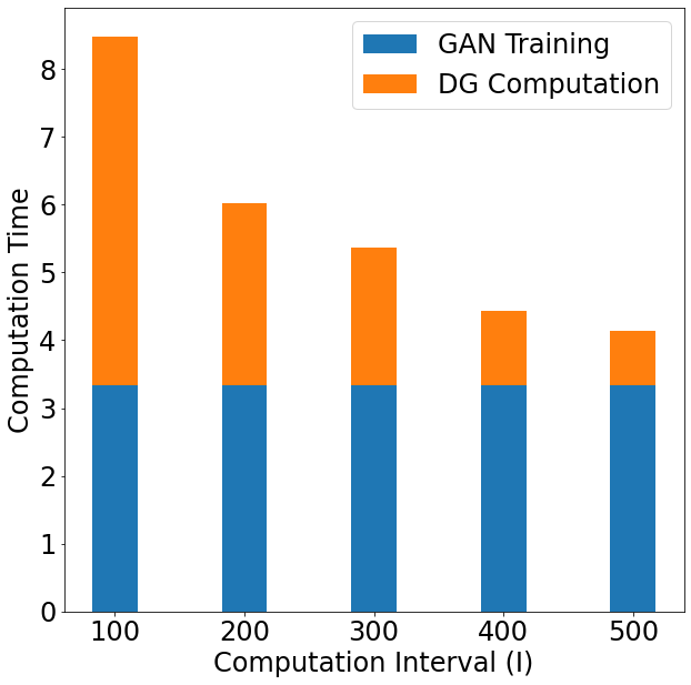
(a)

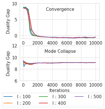
(b)

Figure 6: Computational Complexity (a) Overhead (average time taken per 100 training steps in seconds) of DG estimation at different computation intervals. (b) Perturbed DG captured at different intervals across GAN training process.

We train a classical GAN on the RING dataset. In the first experiment, we track the estimated DG values as a function of auxiliary GAN’s training iterations. Figure 5(b) shows the trend in the perturbed DG values. It is evident from the figure that less than 200 iterations are sufficient for the convergence of the DG for various settings. Figure 6(a) presents the increase in the computational time (averaged over 5 trials) when estimating the DG at various intervals. The number of iterations for training the auxiliary GAN is fixed at 200 as suggested by the early stopping criteria. It can be seen that for higher computation intervals, which are quite practical to work with, the computation time is comparable to the GAN training process without any DG computation. We show that this higher DG computation interval does not degrade the trend captured by the duality gap in figure 6(b). The variance in the DG estimates across the iterations for varying estimation frequency is negligible.

5 Conclusion

Evaluating the training progress of a GAN has been an open problem in the machine learning community. Recently Grnarova et al. establish that the true duality gap is an upper bound on the JS divergence between the real and generated distributions, and through exhaustive experimentation, demonstrate that the duality gap is domain agnostic and can be used to evaluate GANs over a wide variety of tasks. Computing the true duality gap for a GAN is an intractable problem, and thus Grnarova et al. suggest a gradient descent approach to estimate its approximation. This paper shows that the duality gap estimation process suffers from an inherent limitation of being unable to distinguish between Nash and non-Nash attractors of the gradient dynamics associated with the GAN optimization. We present a thorough study of this limitation and propose a method to overcome it without increasing the computational complexity, through local perturbations. Through rigorous experiments, we demonstrate the usefulness of the perturbed duality gap for monitoring GAN training progress. We also show that it is possible to learn generic meta-models capable of driving GANs to convergence using the perturbed duality gap. This potentially opens up new possibilities for automated GAN training.

References

- [1] Ian Goodfellow, Jean Pouget-Abadie, Mehdi Mirza, Bing Xu, David Warde-Farley, Sherjil Ozair, Aaron Courville, and Yoshua Bengio. Generative adversarial nets. In Advances in neural information processing systems, pages 2672–2680, 2014.
- [2] Prateek Jain and Purushottam Kar. Non-convex optimization for machine learning. Foundations and Trends® in Machine Learning, 10, 2017.
- [3] Chun-Liang Li, Wei-Cheng Chang, Yu Cheng, Yiming Yang, and Barnabás Póczos. Mmd gan: Towards deeper understanding of moment matching network. In Advances in Neural Information Processing Systems, pages 2203–2213, 2017.
- [4] Martín Arjovsky, Soumith Chintala, and Léon Bottou. Wasserstein generative adversarial networks. In ICML, volume 70 of Proceedings of Machine Learning Research, pages 214–223. PMLR, 2017.
- [5] Ishaan Gulrajani, Faruk Ahmed, Martin Arjovsky, Vincent Dumoulin, and Aaron C Courville. Improved training of wasserstein gans. In Advances in neural information processing systems, pages 5767–5777, 2017.
- [6] Takeru Miyato, Toshiki Kataoka, Masanori Koyama, and Yuichi Yoshida. Spectral normalization for generative adversarial networks. In ICLR. OpenReview.net, 2018.
- [7] Eric V. Mazumdar, Michael I. Jordan, and S. Shankar Sastry. On finding local nash equilibria (and only local nash equilibria) in zero-sum games. CoRR, abs/1901.00838, 2019.
- [8] Martin Heusel, Hubert Ramsauer, Thomas Unterthiner, Bernhard Nessler, and Sepp Hochreiter. Gans trained by a two time-scale update rule converge to a local nash equilibrium. In Advances in neural information processing systems, pages 6626–6637, 2017.
- [9] Alec Radford, Luke Metz, and Soumith Chintala. Unsupervised representation learning with deep convolutional generative adversarial networks. In ICLR (Poster), 2016.
- [10] Dan Zhang and Anna Khoreva. Progressive augmentation of gans. In Advances in Neural Information Processing Systems 32, pages 6249–6259. 2019.
- [11] Ali Borji. Pros and cons of GAN evaluation measures. CoRR, abs/1802.03446, 2018.
- [12] Mario Lucic, Karol Kurach, Marcin Michalski, Sylvain Gelly, and Olivier Bousquet. Are gans created equal? a large-scale study. In Advances in neural information processing systems, pages 700–709, 2018.
- [13] Catherine Olsson, Surya Bhupatiraju, Tom B. Brown, Augustus Odena, and Ian J. Goodfellow. Skill rating for generative models. CoRR, abs/1808.04888, 2018.
- [14] Lucas Theis, Aäron van den Oord, and Matthias Bethge. A note on the evaluation of generative models. In Yoshua Bengio and Yann LeCun, editors, 4th International Conference on Learning Representations, ICLR 2016, Conference Track Proceedings, 2016.
- [15] Tim Salimans, Ian Goodfellow, Wojciech Zaremba, Vicki Cheung, Alec Radford, and Xi Chen. Improved techniques for training gans. In Advances in neural information processing systems, pages 2234–2242, 2016.
- [16] Mehdi SM Sajjadi, Olivier Bachem, Mario Lucic, Olivier Bousquet, and Sylvain Gelly. Assessing generative models via precision and recall. In Advances in Neural Information Processing Systems, pages 5228–5237, 2018.
- [17] Tuomas Kynkäänniemi, Tero Karras, Samuli Laine, Jaakko Lehtinen, and Timo Aila. Improved precision and recall metric for assessing generative models. In Advances in Neural Information Processing Systems, pages 3927–3936, 2019.
- [18] Ilya O Tolstikhin, Sylvain Gelly, Olivier Bousquet, Carl-Johann Simon-Gabriel, and Bernhard Schölkopf. Adagan: Boosting generative models. In Advances in Neural Information Processing Systems, pages 5424–5433, 2017.
- [19] Muhammad Ferjad Naeem, Seong Joon Oh, Youngjung Uh, Yunjey Choi, and Jaejun Yoo. Reliable fidelity and diversity metrics for generative models. CoRR, abs/2002.09797, 2020.
- [20] Paulina Grnarova, Kfir Y Levy, Aurelien Lucchi, Nathanaël Perraudin, Ian Goodfellow, Thomas Hofmann, and Andreas Krause. A domain agnostic measure for monitoring and evaluating gans. In Advances in Neural Information Processing Systems, pages 12092–12102, 2019.
- [21] Chi Jin, Praneeth Netrapalli, and Michael I. Jordan. What is local optimality in nonconvex-nonconcave minimax optimization?, 2019.
- [22] Anna Choromanska, MIkael Henaff, Michael Mathieu, Gerard Ben Arous, and Yann LeCun. The Loss Surfaces of Multilayer Networks. volume 38 of Proceedings of Machine Learning Research, pages 192–204, 2015.
- [23] Kiran K Thekumparampil, Prateek Jain, Praneeth Netrapalli, and Sewoong Oh. Efficient algorithms for smooth minimax optimization. In Advances in Neural Information Processing Systems, pages 12680–12691, 2019.
- [24] Tanner Fiez, Benjamin Chasnov, and Lillian J. Ratliff. Convergence of learning dynamics in stackelberg games. CoRR, abs/1906.01217, 2019.
- [25] Chi Jin, Rong Ge, Praneeth Netrapalli, Sham M. Kakade, and Michael I. Jordan. How to escape saddle points efficiently. In ICML, volume 70 of Proceedings of Machine Learning Research, pages 1724–1732. PMLR, 2017.
- [26] Li Deng. The mnist database of handwritten digit images for machine learning research. IEEE Signal Processing Magazine, November 2012.
- [27] Han Xiao, Kashif Rasul, and Roland Vollgraf. Fashion-mnist: a novel image dataset for benchmarking machine learning algorithms. CoRR, abs/1708.07747, 2017.
- [28] Alex Krizhevsky, Vinod Nair, and Geoffrey Hinton. Cifar-10 (canadian institute for advanced research). 2014.
- [29] Ziwei Liu, Ping Luo, Xiaogang Wang, and Xiaoou Tang. Deep learning face attributes in the wild. In ICCV, pages 3730–3738. IEEE Computer Society, 2015.
- [30] Haowen Xu, Hao Zhang, Zhiting Hu, Xiaodan Liang, Ruslan Salakhutdinov, and Eric P. Xing. Autoloss: Learning discrete schedule for alternate optimization. In ICLR 2019 (Poster), 2019.