Low-Order Model of Biological Neural Networks

Abstract

A biologically plausible low-order model (LOM) of biological neural networks is a recurrent hierarchical network of models of dendritic nodes/trees, spiking/nonspiking neurons, unsupervised/supervised covariance/accumulative learning mechanisms, feedback connections, and a scheme for maximal generalization. These component models are motivated and necessitated by making LOM learn and retrieve easily without differentiation, optimization or iteration, and cluster, detect and recognize multiple/hierarchical corrupted, distorted and occluded temporal and spatial patterns. A masking matrix for a dendritic tree, whose upper part comprises model dendritic encoders, enables maximal generalization on corrupted, distorted and occluded data. It is a mathematical organization and idealization of dendritic trees with overlapped and nested input vectors. A model nonspiking neuron transmits inhibitory graded signals to modulate its neighboring model spiking neurons. Model spiking neurons evaluate the subjective probability distribution (SPD) of the labels of the inputs to model dendritic encoders, and generate spike trains with such SPDs as firing rates. Feedback connections from the same or higher layers with different numbers of unit-delay devices reflect different signal traveling times, enabling LOM to fully utilize temporally and spatially associated information. Biological plausibility of the component models is discussed. Numerical examples are given to demonstrate how LOM operates in retrieving, generalizing, and unsupervised/supervised learning.

1 Introduction

A learning machine, called a temporal hierarchical probabilistic associative memory (THPAM), was recently reported Lo (2010). The goal to achieve in the construction of THPAM was to develop a learning machine that learns, with or without supervision, and retrieves easily without differentiation, optimization or iteration; and recognizes corrupted, distorted and occluded temporal and spatial information. In the process to achieve the goal, mathematical necessity took precedence over biological plausibility. This top-down approach focused first on minimum mathematical structures and operations that are required for an effective learning machine with the mentioned properties.

THPAM turned out to be a functional model of neural networks with many unique features that well-known models such as the recurrent multilayer perceptron Hecht-Nielsen (1990); Principe et al. (2000); Bishop (2006); Haykin (2009), associative memories Kohonen (1988b); Willshaw et al. (1969); Nagano (1972); Amari (1989); Sutherland (1992); Turner and Austin (1997), spiking neural networks Maass and Bishop (1998); Gerstner and Kistler (2002), and cortical circuit models Martin (2002); Granger (2006); Grossberg (2007); George and Hawkins (2009) do not have.

These unique features indicated that THPAM might contain clues for understanding the operations and structures of biological neural networks. The components of THPAM were then examined from the biological point of view with the purpose of constructing a model of biological neural networks with biologically plausible component models. The components of THPAM were identified with those of biological neural networks and reconstructed, if necessary, into biologically plausible models of the same.

This effort resulted in a low-order model (LOM) of biological neural networks. LOM is a recurrent hierarchical network of biologically plausible models of dendritic nodes and trees, synapses, spiking and nonspiking neurons, unsupervised and supervised learning mechanisms, a retrieving mechanism, a generalization scheme, and feedback connections with delays of different durations. All of these biologically plausible component models, except the generalization scheme and the feedback connections, are significantly different from their corresponding components in THPAM. More will be said about the differences.

Note that although a dendrite or axon is a part of a neuron, and a dendro-dendritic synapse is a part of a dendrite (thus a part of a neuron), they are treated, for simplicity, as if they were separate entities, and the word “neuron” refers essentially to the soma of a neuron in this paper.

A basic approximation made in the modeling effort reported here is that LOM is a discrete-time model and all the spike trains running through it are Bernoulli processes. The discrete-time approximation is frequently made in neuroscience. Mathematically, Bernoulli processes are discrete-time approximation of Poisson processes, which are usually used to model spike trains. The discrete-time assumption seems similar to that made in the theory of discrete-time dynamical systems as exemplified by the standard time-discretization of a differential equation into a difference equation. However, it is appropriate to point out that the discrete time for LOM and Bernoulli processes is perhaps more than simply a mathematical approximation.

1. A spike (or action potential) is not allowed to start within the refractory period of another, violating a basic property of Poisson processes. Consecutive spikes in the brain cannot be arbitrarily close and are separated at least by the duration of a spike including its refractory period, setting the minimum time length between two consecutive time points in a time line.

2. Neuron or spike synchronization has been discovered in biological neural networks Von der Malsburg (1981); Singer and Gray (1995). Such synchronization may originate from or be driven by synchronous spikes from sensory neurons.

3. If a neuron and its synapses integrate multiple spikes in response to sensory stimuli being held constant (e.g., an image fixated by the retina for about 1/3 of a second), and the neuron generates multiple spikes in the process of each of such integrations; different time scales and their match-up can probably be reconciled for the discrete-time LOM and Bernoulli processes. Before more can be said, the discrete-time approximation is looked upon as part of the low-order approximation by LOM.

2 Brief Description of LOM

LOM is a layered network of processing units (PUs), which is actually rather simple in structure and operation. Each PU is composed of a number of (model) spiking neurons that jointly output a binary estimate of the label of the image appearing in the receptive fiels of the PU. Each neuron contains dendrites, synapses, spiking/nonspiking somas, Hebbian learning mechanisms, and generalization schemes, which are of course all computational models.

As a image appears in the receptive field of a PU, the image is encoded by the dendrites into a dendritic code. If the outer product of this code and the label estimate output from the PU is added to the memories stored in the synapses completing the unsupervised Hebbian learning of the image input to the PU, the PU is called a UPU (unsupervised PU). If the label estimated is replaced with a label provided from outside of the PU in learning the input image, the supervised Hebbian learning is completed and the PU is called an SPU (supervised PU). Different dendritic codes are orthogonal, allowing us to decode the dendritic code of the estimated or provided label for retrieving the same.

2.1 Encoding inputs to neurons

Dendritic trees use more than 60% of the energy consumed by the brain Wong (1989), occupy more than 99% of the surface of some neurons Fox and Barnard (1957), and are the largest component of neural tissue in volume Sirevaag and Greenough (1987). Yet, dendritic trees are missing in deep learning machines (including convolutional neural networks), associative memories Kohonen (1988a); Hinton and Anderson (1989); Hassoun (1993) and models of cortical circuits Martin (2002); Granger (2006); Grossberg (2007); George and Hawkins (2009), overlooking a large proportion of the neuronal circuit.

A key feature of LOM is a novel model of the dendritic encoder. A dendritic encoder that inputs $v_{\tau}=\left[\begin{array}[]{ccc}v_{\tau 1}&v_{\tau 2}&v_{\tau 3}\end{array}\right]^{\prime}$ encodes it into the dendritic code $\breve{v}_{\tau}$ by the standard parity function $\phi$ as follows: $\breve{v}_{\tau}=$ $[0\quad v_{\tau 1}\quad v_{\tau 2}\quad$ $\phi\left(v_{\tau 2},v_{\tau 1}\right)$ $v_{\tau 3}\quad\phi\left(v_{\tau 3},v_{\tau 1}\right)\quad$ $\phi\left(v_{\tau 3},v_{\tau 2}\right)$ $\quad\phi\left(v_{\tau 3},v_{\tau 2},v_{\tau 1}\right)]^{\prime}$

A graph showing the dendritic encoder is given in Figure. 1. For example, $\left[\begin{array}[]{ccc}1&0&1\end{array}\right]^{\prime}$ and $\left[\begin{array}[]{ccc}0&1&1\end{array}\right]^{\prime}$ are encoded into the codes $\left[\begin{array}[]{cccccccc}0&1&0&1&1&0&1&0\end{array}\right]^{\prime}$ and $\left[\begin{array}[]{cccccccc}0&0&1&1&1&1&0&0\end{array}\right]^{\prime}$ respectively.

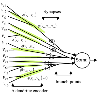
Figure 1: A dendritic encoder.

In general, given an input vector $v_{\tau}$ = $\left[v_{\tau 1},\ldots,v_{\tau m}\right]^{\prime}$ to a dendritic encoder, the dendritic code $\breve{v}_{\tau}$ of the vector $v_{\tau}$ is $[0\quad v_{\tau 1}\quad v_{\tau 2}\quad\phi\left(v_{\tau 2},v_{\tau 1}\right)\quad$ $v_{\tau 3}\quad\phi\left(v_{\tau 3},v_{\tau 1}\right)\quad\phi\left(v_{\tau 3},v_{\tau 2}\right)\quad\phi\left(v_{\tau 3},v_{\tau 2},v_{\tau 1}\right)\quad$ $\cdots\quad\phi\left(v_{\tau m},\cdots,v_{\tau 1}\right)]^{\prime}$ Dendritic codes have the orthogonality property: If $v_{\tau}\neq v_{t}$, then $\left(\breve{v}_{\tau}-\frac{1}{2}\mathbf{1}\right)^{\prime}\left(\breve{v}_{t}-\frac{1}{2}\mathbf{1}\right)=0$. If $v_{\tau}=v_{t}$, then $\left(\breve{v}_{\tau}-\frac{1}{2}\mathbf{1}\right)^{\prime}\left(\breve{v}_{t}-\frac{1}{2}\mathbf{1}\right)=2^{\dim v_{\tau}-2}$, where 1 = $\left[\begin{array}[]{cccc}1&1&\cdots&1\end{array}\right]^{\prime}$. This key property is proven in Lo (2011). To avoid curse of dimensionality and enhance generalization capability, only subvectors of the feature vector $v_{\tau}$ are expanded as above.

2.2 Unsupervised/supervised learning and memorizing in synapses

Figure 2: Unsupervised covariance learning.

Figure. 2 shows the output $\breve{v}_{tj}$ of the dendritic encoder going through a synapse with weight $D_{ij}$ represented by $\otimes$ to reach spiking soma $i$, whose output at time $t$ is $u_{ti}$.The unsupervised covariance rule that updates the strength $D_{ij}$ of the synapse receiving $\breve{v}_{tj}$ and feeding spiking neuron $i$ whose output is $u_{ti}$ follows:

$$D_{ij}\leftarrow\lambda D_{ij}+\Lambda\left(u_{ti}-\left\langle u_{ti}\right\rangle\right)\left(\breve{v}_{tj}-\left\langle\breve{v}_{tj}\right\rangle\right)$$ (1)

where $\Lambda$ is a proportional constant, $\lambda$ is a forgetting factor that is a positive number less than one, and $\left\langle\breve{v}_{tj}\right\rangle$ and $\left\langle u_{ti}\right\rangle$ denote, respectively, the average activities of the presynaptic dendritic node $j$ and postsynaptic spiking neuron $i$ over some suitable time intervals.

The outputs $u_{ti}$, $i=1,\ldots,R,$ of the $R$ spiking somas can be assembled into a vector, $u_{t}$ = $\left[\begin{array}[]{cccc}u_{t1}&u_{t2}&\cdots&u_{tR}\end{array}\right]^{\prime}$, and the strengths $D_{ij}$ into a matrix $D$ whose $i\times j$-th entry is $D_{ij}$. The vector $u_{t}$ is the label of the input vector $v_{t}$ that is selected in accordance with a probability distribution or membership function by the neurons for unsupervised learning Lo (2011). Such selection creates a vocabulary for the neurons themselves.

The synaptic strengths on the connections from the output terminals of a dendritic encoder to a single nonspiking neuron form a row vector $C$ and are updated by the unsupervised accumulation rule:

$$C\leftarrow\lambda C+\frac{\Lambda}{2}\left(\breve{v}_{t}-\left\langle\breve{v}_{t}\right\rangle\right)^{\prime}$$ (2)

For supervised learning, the output $u_{ti}$ from the spiking soma $i$ in (1) is replaced with a component $w_{ti}$ of the label of the input vector $v_{t}$ provided from outside the LOM. Note that the label is that of the feature vector in the receptive field of soma $i$.

2.3 Masking Matrices for Generalization

If the vector $v_{\tau}$ input to a neuron has not been learned (possibly due to distortion, corruption and occlusion), it would be ideal if the largest subvector of $x_{\tau}$ that matches at least one subvector $x_{t}$ stored in the $D$ and $C$ stored in the synapses can be found automatically and the subjective probability distribution of the label of this largest subvector of $x_{\tau}$ can be generated. This ideal capability is called maximal/adjustable generalization. Maximal generalization can actually be achieved by the use of a masking matrix $M$.

For example, masking the second and fourth components of $\mathbf{1}=\left[\begin{array}[]{ccccc}1&1&1&1&1\end{array}\right]^{\prime}$ can be done with the multiplication $diag\left[\begin{array}[]{ccccc}1&0&1&0&1\end{array}\right]\mathbf{1}$ by the masking matrix $diag\left[\begin{array}[]{ccccc}1&0&1&0&1\end{array}\right]$. Masking certain numbers of bits and assigning different weights to the corresponding masking matrices to deemphasize masking large numbers of bits allow us to achieve maximal/adjustable generalization. Detailed description of masking matrices can be found in Lo (2011).

2.4 Estimation of labels by Somas

Once a vector $v_{\tau}$ is received and encoded by a dendritic encoder into $\breve{v}_{\tau}$, $\breve{v}_{\tau}$ is made available to synapses for learning as well as retrieving of the information about the label of the input $v_{\tau}$. In response to $\breve{v}_{\tau}$, the masking matrix $M$ computes $M_{jj}\left(\breve{v}_{\tau j}-\left\langle\breve{v}_{\tau j}\right\rangle\right)$ for all $j$.

Figure 3: Nonspiking soma and spiking soma k.

Synapse $j$ for a nonspiking soma then computes $c_{\tau j}=C_{j}M_{jj}\left(\breve{v}_{\tau j}-\left\langle\breve{v}_{\tau j}\right\rangle\right)$, for all $j$, where $M_{jj}$ is the $j$-th diagonal entry of $M$. As shown in Figure. 3, the model nonspiking soma sums up $c_{\tau j}$ to obtain the graded signal $c_{\tau}$. Note that the synaptic weight vector $C$ is defined in (2). Because of the orthogonality property of $\breve{v}_{\tau}$, $t$ = 1, …, $T$; $c_{\tau}$ is an estimate of the total number of times $\breve{v}_{\tau}$ has been encoded and stored in $C$. The inhibitory output $-c_{\tau}$is a graded signal transmitted to each of the mentioned $R$ spiking neurons that generate a point estimate of the label $r_{t}$ of $v_{\tau}$.

The model spiking soma $k$ is also depicted in Figure. 3. The entries of the $j$th row $D_{j}$ of $D$ are the weights or strengths of the synapses for the $j$th spiking neuron. In response to $\breve{v}_{\tau}$ produced by the dendritic encoders, the masking matrix $M$ and synapses for the $j$th spiking neuron compute $M_{jj}\left(\breve{v}_{\tau j}-\left\langle\breve{v}_{\tau j}\right\rangle\right)$ and $d_{\tau kj}$ = $D_{kj}M_{jj}\left(\breve{v}_{\tau j}-\left\langle\breve{v}_{\tau j}\right\rangle\right)$, respectively. As shown in Figure 3, the $j$th spiking neuron (a model spiking neuron) sums up $d_{\tau kj}$ to obtain the graded signal $d_{\tau k}$ = $\sum_{j}d_{\tau kj}$.

Because of the orthogonality property of $\breve{v}_{\tau}$; $d_{\tau k}$ is an estimate of the total number of times $v_{\tau}$ has been encoded and stored in $D_{k}$ with the $k$th component $r_{\tau k}$ of $r_{\tau}$ being 1 minus the total number of times $v_{\tau}$ has been encoded and stored in $D_{k}$ with the $k$th component $r_{\tau k}$ of $r_{\tau}$ being $0$. The effects of $M$, $\lambda$ and $\Lambda$ are included in computing said total numbers, which make $d_{\tau k}$ only an estimate.

Recall that $c_{\tau}$ is an estimate of the total number of times $v_{\tau}$ has been learned regardless of its labels. Therefore, $\left(c_{\tau}+d_{\tau k}\right)/2$ is an estimate of the total number of times $v_{\tau}$ has been encoded and stored with the $k$th component $r_{\tau k}$ of $r_{\tau}$ being 1. Consequently, $\left(d_{\tau k}/c_{\tau}+1\right)/2$ is the subjective probability $p_{\tau k}$ that $r_{\tau k}$ is equal to 1. The $k$th spiking neuron then uses a pseudo-random generator to generate 1 with probability $p_{\tau j}$ and $0$ with probability $1-$ $p_{\tau j}$. This 1 or $0$ is the output of the $k$th spiking neuron. Biological justification of the model nonspiking and spiking somas are provided in Lo (2011).

Note that the vector $p_{\tau}=\left[\begin{array}[]{cccc}p_{\tau 1}&p_{\tau 2}&\cdots&p_{\tau R}\end{array}\right]^{\prime}$ is a representation of a subjective probability distribution of the label $r_{\tau}$ of the input vector $v_{\tau}$. A pseudorandom ternary number generator in the $j$th spiking neuron uses $p_{\tau j}$ to generate an output denoted by $v\left\{p_{\tau k}\right\}$ as follows: $v\left\{p_{\tau k}\right\}$ = 1 with probability $p_{\tau k}$, and $v\left\{p_{\tau k}\right\}$ = $-1$ with probability $1-p_{\tau k}$. Note also that the outputs of the $R$ spiking neurons in response to $v_{\tau}$ form a binary vector $v\left\{p_{\tau}\right\}$, which is a point estimate of the label $r_{\tau}$ of $v_{\tau}$.

2.5 Processing Units (PUs)

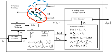
Figure 4: Unsupervised or supervised processing unit (UPU or SPU).

LOM organizes a biological neural network into a recurrent network of PUs (processing units). A schematic diagram of a PU is shown in Figure. 4, which shows how dendritic encoders, synapses, a nonspiking soma, $R$ spiking somas, and learning and retrieving mechanisms are integrated into a processing unit (PU). The vector $v_{\tau}$ input to a PU is first expanded by dendritic encoders into a dendritic code $\breve{v}_{\tau}$. $\ \breve{v}_{\tau}$ is used to compute $c_{\tau j}$ and $d_{\tau kj}$ using the synaptic weights $C_{j}$ and $D_{kj}$ respectively. The nonspiking soma in the PU computes the sum $\sum\limits_{j}c_{\tau j}$, and the $k$th spiking soma computes $\sum\limits_{j}d_{\tau kj}$ and $p_{\tau k}$ = $\left(\sum\limits_{j}d_{\tau kj}/\sum\limits_{j}c_{\tau j}+1\right)/2$, which is the relative frequency that the $k$th digit of the label of $v_{\tau}$ is +1. By a pseudo-random generator, the $k$th spiking soma outputs $v\left\{p_{\tau k}\right\}$, which is +1 with probability $p_{\tau k}$ and is $-1$ with probability 1 $-$ $p_{\tau k}$, for $k$ = 1, …, $R$. $v\left\{p_{\tau}\right\}$ = $\left[\begin{array}[]{ccc}v\left\{p_{\tau 1}\right\}&\cdots&v\left\{p_{\tau R}\right\}\end{array}\right]^{\prime}$ is a point estimate of the label of $v_{\tau}$. Note that use of weights in the masking matrices can facilitate max-pooling of dendritic encoders in the computation of $p_{\tau k}$ Lo (2011).

The green lever circled with the red solid line indicates that the estimated label $v\left\{p_{\tau}\right\}$ is used for unsupervised learning. In this case, the PU is a unsupervised PU (UPU). If the green lever is placed in the position circled with the blue dashed line, then the handcrafted $r_{\tau}$ is used for supervised learning, and the PU is a supervised PU (SPU). UPUs in the lowest layer cluster and recognize the lowest level of pattern elements such as variants of a hyphen, a pipe, a slash, a back slash, and so on. These pattern elements are integrated from layer to layer into larger and larger pattern elements and patterns. As long as inputs are provided to an UPU by sensors or other parts of the LOM, the UPU learns (without supervision).

By the maximal/adjustable generalization capability (or more specifically, masking matrix $M$), each UPU acts as a cluster of its input vectors $v_{\tau}$. If $v_{\tau}$ or a close version has not been learned by an UPU, The UPU generates the label of $v_{\tau}$ at random. This enables the UPU to act as a pattern recognizer by itself. Whenever a handcrafted label $r_{\tau}$ is available to an SPU, the SPU learns its input vector $v_{\tau}$ with $r_{\tau}$. By the maximal/adjustable generalization capability, the entire cluster(s) constructed by the UPU(s) that provide $v_{\tau}$ is assigned the same label $r_{\tau}$. This minimizes the amount of handcrafted labels required.

2.6 Clustering and Interpreting

The version of LOM proposed herein consists of a hierarchical network of UPUs (unsupervised processing units) with feedbacks connections, acting as pattern recognizers, and a number of offshoot SPUs (supervised processing units), translating the self-generated labels from UPUs into human language, which are called the clusterer and interpreter, respectively. An example clusterer in its entirety for clustering spatial and temporal data is shown in Figure. 5. The feedback connections in the clusterer have delay devices of different durations make LOM suitable for recognizing temporal patterns in video and movie. However, they will not be used in the proposed project.

Once an exogenous feature vector is input to the clusterer, the UPUs perform retrieving and/or learning from layer to layer starting with layer 1, the lowest layer. After the UPUs in the highest layer complete performing their functions, the clusterer is said to have completed one round of retrievings and/or learnings (or memory adjustments). For each exogenous feature vector, the clusterer will continue to complete a certain number of rounds of retrievings and/or learnings.

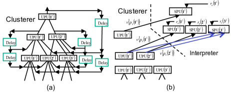
Figure 5: (a)A network of unsupervised processing units(UPUs), (b) offshoot supervised processing units(SPUs)

The clusterer in Figure. 5 (a) is also shown in Figure. 5 (b) with the connections and delay devices removed. The three UPUs in the lowest layer of the clusterer do not branch out, but each of the three UPUs in the second and third layers branches out to an SPU. UPU$\left(\mathbf{1}^{2}\right)$ and UPU$\left(\mathbf{2}^{2}\right)$ in the second layer have feedforward connections to SPU$\left(\mathbf{1}^{2}\right)$ and SPU$\left(\mathbf{2}^{2}\right)$ respectively, and UPU$\left(\mathbf{1}^{3}\right)$ in the third layer has feedforward connections to SPU$\left(\mathbf{1}^{3}\right)$.

The labels, $r_{\tau}\left(\mathbf{1}^{2}\right)$, $r_{\tau}\left(\mathbf{2}^{2}\right)$ and $r_{\tau}\left(\mathbf{1}^{3}\right)$, which are used for supervised learning are provided by the human trainer of the LOM.

3 Preliminary Numerical Tests of LOM

3.1 A simplified supervised learning architecture based on LOM

This section describes in detail the architecture of a simplified LOM supervised learning neural network model. This architecture comprises four layers, including the input layer, output layer, and two hidden layers. The inputs are $28\times 28$ pixel images from the standard MNIST database. In the input layer, a $28\times 28$ pixel image is split into 22 per row and 22 per column sub-images, the total number of sub-images is $22\times 22=484$. The sub-images are generated by sliding an $8\times 8$ pixel window one row or one column each time. An input prepared for a first hidden layer PU is a manually selected16-pixel pattern from the $8\times 8$ pixel sub-image. The selection pattern for each first hidden layer PU is identical. Each PU in each layer is fixed and is always focusing on the same receptive field of the images during the training and testing process.

The input pixels’ values are normalized so that the white $(0)$ corresponds to a grayscale value of smaller than 35, and the black $(1)$ corresponds to a grayscale value of larger or equal to 35, which fits the learning scheme. The second hidden layer consists $11\times 11=121$ PUs. The input of a PU is formed by combining the output of four lower hidden layer PUs. The lower layer’s four PUs are the closest neighbors form a square without overlapping each other. In this case, the receptive field of a PU in the current layer is extended to $16\times 16$.

Within the hidden layers, supervised learning is applied. In the first hidden layer, before a pattern is prepared as an input to be learned by the hidden layer PU, the PU will first check whether the neurons have seen this pattern. If the pattern has not been learned before, this pattern will be learned using the image’s 4-bit binary label, translated from the original 0-9 decimal label. However, if the pattern has been seen before, the neurons can retrieve the pattern’s label by translating probabilities into a label. This pre-check garnered one pattern that does not have two or more labels, which greatly confuse the PU when retrieving. This schema is based on the that the digits share many similar parts. We do not need to distinguish each part in every digit. What we really care about is that the pattern is represented following the right way. For example, if a digit can be covered by the receptive field of four square PUs in the first hidden layer, because the top arch pattern of the $"2"$ and $"3"$ are similar, the label retrieved from the top two PUs of the four PUs will tell the PU of the next layer this digit is an arch pattern, but they are not sure whether it is from $"2"$ or $"3"$. After gathering all the four PUs, the PU of the next layer can finally give a prediction based on the patterns shown in each part of the digit.

The second hidden layer does not apply the same learning scheme. In the learning process, a decimal label is translated as a 10-bit one-hot label. Whether the input has been learned or not, it will be learned with the label of the current image. That implies that the same pattern might have two or more labels assigned to it. In the testing process, the 10-bit probability vectors will be treated as the output of the PU.

In the final output layer, each second hidden layer’s prediction was analyzed and summarized to produce a final prediction. Each probability vectors will check whether the biggest probability within the vector is larger than 0.85. If the vector’s largest probability is smaller than 0.85, that means this pattern might have been assigned many labels and will produce ambiguities towards the final prediction. To obtain a more reliable result, only the vectors with the biggest probability larger than 0.85 will be summed up in the final layer. Finally, the biggest probability after summation will decide the result.

3.2 Tests on the MNIST dataset

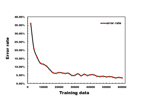
Figure 6: Error rate of real-time learning.

The above architecture is developed and tested on the standard. MNIST dataset consists of 60,000 images of handwritten numerals for training and 10,000 images for testing, each image containing 28$\times$28 pixels. The 60,000 images are divided into 30 bins. Each bin consists of 2000 images. The real-time learning machine-learned each bin sequentially. After learning every 2000 images, the learning machine uses the 10,000 testing images to make a prediction. Following this procedure, a total of 30 predictions of the testing data are made. As shown in Figure. 6. the error rate of each prediction is marked as a red dot. There is an overall downward trend. The error rate drops dramatically from 37% to lower than 10%, with only learning the first 12,000 training images. The downward trend slowed down afterward. The final error rate is 3.28%. The error rate continually dropping around 1% over the learning procedure of the last 10,000 training images confirmed the LOM model’s potential and showed room for improvement. We expect that new LOM architectures will soon be found to achieve an accuracy rate close to the best error rate. It is appropriate to note that MNIST is a fixed collection of images of handwritten numerals, each with a single given hand-crafted label, on which training a learning machine requires none of the above desirable learning capabilities. MNIST is, therefore, an ideal kind of dataset for deep learning machine to be trained on without limits on the number of training sessions, the number of times the weights of deep learning machine can be changed, or the training time in each training session. However, this proposal’s main objective is to develop highly accurate LOM architectures with capabilities of real-time, photographic, unsupervised, and hierarchical learning.

References

- Amari [1989] S. Amari. Characteristics of sparsely encoded associative memory. Neural Networks, 2(6):451–457, 1989.
- Bishop [2006] C. M. Bishop. Pattern Recognition and Machine Learning. Springer Science, New York, 2006.
- Fox and Barnard [1957] C. A. Fox and J. W. Barnard. A quantitative study of the purkinje cell dendritic branches and their relationship to afferent fibers. Journal of Anatomy, 91:299–313, 1957.
- Fromherz and Gaede [1993] Peter Fromherz and Volker Gaede. Exclusive-or function of single arborized neuron. Biological Cybernetics, 69:337–334, 1993.
- Gabbiani et al. [2002] F. Gabbiani, H. G. Krapp, C. Koch, and G. Laurent. Multiplication computation in a visual neuron sensitive to looming. Nature, 420:320–324, 2002.
- Gabbiani et al. [2004] F. Gabbiani, H. G. Krapp, N. Hatsopoulos, C.-H. Mo, C. Koch, and G. Laurent. Multiplication and stimulus invariance in a looming-sensitive neuron. Journal of Physiology, 98:19–34, 2004.
- George and Hawkins [2009] D. George and J. Hawkins. Towards a mathematical theory of cortical micro-circuits. PLoS Computational Biology, 5-10:1–26, 2009.
- Gerstner and Kistler [2002] W. Gerstner and W. M. Kistler. Spiking Neuron Models, Single Neurons, Populations, Plasticity. Cambridge University Press, Cambridge, UK, 2002.
- Granger [2006] R. Granger. Engines of the brain: The computational instruction set of human cognition. AI Magazine, 27:15–31, 2006.
- Grossberg [2007] S. Grossberg. Towards a unified theory of neocortex: Laminar cortical circuits for vision and cognition. Progress in Brain Research, 165:79–104, 2007.
- Hassoun [1993] M. H. Hassoun. Associative Neural Memories, Theory and Implementation. Oxford University Press, New York, New York, 1993.
- Haykin [2009] Simon Haykin. Neural Networks and Learning Machines, Third Edition. Prentice Hall, Upper Saddle River, New Jersey, 2009.
- Hecht-Nielsen [1990] Robert Hecht-Nielsen. Neurocomputing. Addison-Wesley Publishing Company, New York, NY, 1990.
- Hinton and Anderson [1989] G. E. Hinton and J. A. Anderson. Parallel Models of Associative Memory. Lawrence Erlbaum Associates, Hillsdale, New Jersey, 1989.
- Kalman et al. [1969] R. E. Kalman, P. Falb, and M. A. Arbib. Topics in Mathematical System Theory. McGraw-Hill, New York, 1969.
- Koch and Poggio, et al. [1983] C. Koch and T. Poggio, et al. Nonlinear interactions in a dendritic tree: localization, timing, and role in information processing. Proceedings of National Academy of Sciences, U.S.A., 80(9):2799–2802, 1983.
- Koch and Poggio [1982] C. Koch and T. Poggio. Retina ganglion cells: a functional interpretation of dendritic morphology. Philos Trans R Soc Lond B Biol Sci, 298(1090):227–263, 1982.
- Koch and Poggio [1992] C. Koch and T. Poggio. Multiplying with synapses and neurons. In T. McKenna, J. Davis, and S. F. Zornetzer, editors, Single Neuron Computation. Academic Press, Boston MA, 1992.
- Koch [1999] Christof Koch. Biophysics of Computation. Oxford University Press, 1999.
- Kohonen [1988a] T. Kohonen. Self-Organization and Associative Memory. Springer Verlag, New York, New York, 1988.
- Kohonen [1988b] T. Kohonen. Self-Organization and Associative Memory, second edition. Springer-Verlag, New York, 1988.
- Landau and Lifshitz [1987] L. D. Landau and E. M. Lifshitz. Fluid mechanics. Pergamon Press, 1987.
- Lo [2010] James Ting-Ho Lo. Functional model of biological neural networks. Cognitive Neurodynamics, 4-4:295–313, Published online 20 April 2010, 2010.
- Lo [2011] James Ting-Ho Lo. A low-order model of biological neural networks. Neural Computation, 23-10:2626–2682, 2011.
- Maass and Bishop [1998] W. Maass and C. M. Bishop. Pulsed Neural Networks. The MIT Press, Cambridge, Massachussetts, 1998.
- Martin [2002] Kevan A. C. Martin. Microcircuits in visual cortex. Current Opinion in Neurobiology, 12-4:418–42, 2002.
- Mel [1992a] B. W. Mel. The clusteron: toward a simple abstraction in a complex neuron. In J. Moody, S. Hanson, and R. Lippmann, editors, Advances in Neural Information Processing Systems, volume 4, pages 35–42. Morgan Kauffmann, San Mateo, CA, 1992.
- Mel [1992b] B. W. Mel. NMDA-based pattern discrimination in a modeled cortical neuron. Neural Computation, 4:502–516, 1992.
- Mel [1993] B. W. Mel. Synaptic integration in an excitable dendritic tree. Journal of Neurophysiology, 70(3):1086–1101, 1993.
- Mel [1994] B. W. Mel. Information processing in dendritic trees. Neural Computation, 6:1031–1085, 1994.
- Mel [2008] B. W. Mel. Why have dendrites? a computational perspective. In Greg Stuart, Nelson Spruston, and Michael Hausser, editors, Dendrites, Second Edition. Oxford University Press, Oxford, United Kingdom, 2008.
- Nagano [1972] K. Nagano. Association - a model of associative memory. IEEE Transactions on Systems, Man and Cybernetics, SMC-2:68–70, 1972.
- Principe et al. [2000] J. C. Principe, N. R. Euliano, and W. C. Lefebvre. Neural and Adaptive Systems: Fundamentals through Simulations. John Wiley and Sons, Inc., New York, 2000.
- Rall and Sergev [1987] W. Rall and I. Sergev. Functional possibilities for synapses on dendrites and on dendritic spines. In G. M. Edelman, W. F. Gail, and W. M. Cowan, editors, Synaptic Function, pages 603–636. Wiley, New York, 1987.
- Schlichting and Gersten [2000] H. Schlichting and K. Gersten. Boundary-Layer Theory. Springer, New York, 2000.
- Sejnowski [1977] T. J. Sejnowski. Storing covariance with nonlinearly interacting neurons. Journal of Mathematical Biology, 69:303–321, 1977.
- Shepherd and Brayton [1987] G. M. Shepherd and R. K. Brayton. Logic operations are properties of computer-simulated interactions between excitable dendritic spines. Neuroscience, 21(1):151–165, 1987.
- Singer and Gray [1995] W. Singer and C. M. Gray. Visual feature integration and the temporal correlation hypothesis. Annual Review of Neuroscience, 18:555, 1995.
- Sirevaag and Greenough [1987] A. M. Sirevaag and W. T. Greenough. Differential rearing effects on rat visual cortex synapses, III neuronal and glial nuclei, boutons, dendrites, and capillaries. Brain Research, 424:320–332, 1987.
- Sutherland [1992] J. G. Sutherland. The holographic neural method. In Soucek Branko, editor, Fuzzy, Holographic, and Parallel Intelligence. John Wiley and Sons, 1992.
- Tal and Schwartz [1997] D. Tal and E. L. Schwartz. Computing with the leaky integrate and fire neuron: logarithmic computation and multiplication. Neural Computation, 9(2):305–318, 1997.
- Turner and Austin [1997] M. Turner and J. Austin. Matching performance of binary correlation matrix memories. Neural Networks, 1997.
- Von der Malsburg [1981] C. Von der Malsburg. The correlation theory of brain function. In E. Domani, J. L. Van Hemmen, and K. Schulten, editors, Models of neural networks II. Springer, Berlin, 1981.
- Willshaw et al. [1969] D. J. Willshaw, O. P. Buneman, and H. C. Longet-Higgins. Non-holographic associative memory. Nature, 222:960–962, 1969.
- Wong [1989] M. T. T. Wong. Cytochrome oxidase: an endogenous metabolic marker for neuronal activity. Trends in Neuroscience, 12(3):94–101, 1989.
- Zador et al. [1992] Anthony M. Zador, Brenda J. Clairborne, and Thomas H. Brown. Nonlinear pattern separation in single hippocampal neurons with active dendritic membrane. In J. Moody, Hanson S, and R. Lippmann, editors, Advances in Neural Information Processing Systems, volume 4, pages 51–58. Morgan Kaufmann, San Mateo, CA, 1992.