A Perturbation Approach to
Optimal Investment, Liability Ratio, and Dividend Strategies

Abstract

We study an optimal dividend problem for an insurer who simultaneously controls investment weights in a financial market, liability ratio in the insurance business, and dividend payout rate. The insurer seeks an optimal strategy to maximize her expected utility of dividend payments over an infinite horizon. By applying a perturbation approach, we obtain the optimal strategy and the value function in closed form for log and power utility. We conduct an economic analysis to investigate the impact of various model parameters and risk aversion on the insurer’s optimal strategy.

Keywords: Jump Diffusion; Optimal Dividend; Reinsurance; Stochastic Control

1 Introduction

Stochastic control has enjoyed great success in actuarial science since 1990s; see, e.g., Browne, (1995) and Asmussen and Taksar, (1997) for early contributions and the monograph Schmidli, (2007) for a more systematic overview. Of particular interest in the application of stochastic control to actuarial problems is the study of optimal dividend strategies for an insurer. In this paper, we consider an insurer who controls not only dividend payments but also investment and liability strategies simultaneously, and apply a perturbation approach to solve such an optimization problem under the utility maximization criterion.

The optimal dividend problem is a well-studied topic that, generally speaking, seeks an optimal dividend strategy so as to optimize the insurer’s business objective. In a seminal paper, De Finetti, (1957) models the insurer’s risk process $R$ under the classical Cremér-Lundberg (CL) setting and considers an insurer who seeks to maximize the expected discounted dividend payments until the ruin time $\tau$:

(1.1) $$\max\;\int_{0}^{\tau}\,e^{-\delta t}\,\mathrm{d}\widetilde{D}_{t},$$

where $\delta>0$ is the (subjective) discount rate and $\widetilde{D}=(\widetilde{D}_{t})_{t\geq 0}$ denotes the insurer’s dividend strategy, with $\widetilde{D}_{t}$ representing the cumulative dividend payments up to time $t$. Note that the ruin time $\tau$ in (1.1) depends on the dividend strategy $\widetilde{D}$; let us denote $X=X^{\widetilde{D}}$ the insurer’s controlled surplus (wealth) process, then $\tau=\tau^{\widetilde{D}}:=\inf\{t:X^{\widetilde{D}}\leq 0\}$. The optimal dividend strategy $\widetilde{D}^{*}$ to Problem (1.1) is often a band strategy and may further reduce to a barrier strategy in certain cases; see Avanzi, (2009) for details. There is a rich body of literature on the optimal dividend problem by now; see Schmidli, (2007)[Sections 2.4 and 2.5] for a standard textbook treatment. We refer readers to Albrecher and Thonhauser, (2009) and Avanzi, (2009) for more comprehensive surveys on this topic. In what follows, we conduct a selective literature review on this problem by discussing various extensions to the work of De Finetti, (1957) from four different angles: the risk model, the type of dividend strategies, additional control components and constraints, and the optimization objective.

First, we discuss extensions to De Finetti, (1957) in the modeling of the insurer’s risk and (uncontrolled) surplus processes. When it comes to the modeling of the insurer’s risk process $R$, a popular choice is the diffusion model, which can be seen as a continuous approximation to the classical CL model. Please see Jeanblanc-Picqué and Shiryaev, (1995), Asmussen and Taksar, (1997), Højgaard and Taksar, (1999), and Choulli et al., (2003), among many others for investigations of optimal dividend under the diffusion risk model. Further generalizations to the standard diffusion model include incorporating mean-reverting (see Cadenillas et al., (2007) and Avanzi and Wong, (2012)) and regime switching (see Sotomayor and Cadenillas, (2011) and Jin et al., (2013)). Much of the attention in modeling goes to the risk process $R$, while less is concerned about the premium process $p=(p_{t})_{t\geq 0}$. In most analyses, $p_{t}$ is a constant (see, e.g., Taksar and Zhou, (1998) and Azcue and Muler, (2005)) or further given by a specific premium principle (see, e.g., Asmussen et al., (2000) for the expected value principle). But other studies apply a stochastic process (e.g., a diffusion or jump-diffusion process) to model the insurer’s surplus without dividend; see, e.g., Choulli et al., (2003), Gerber and Shiu, (2004), Cadenillas et al., (2007), Chen et al., (2014), and Zhu, (2015). Opposite to the standard risk model is the so-called dual risk model, where $p$ is now the expense rate and $R$ is interpreted as the positive gains. Optimal dividend in the dual model is studied in Avanzi et al., (2007), Avanzi and Gerber, (2008), and Bayraktar et al., (2013, 2014), among others.

Second, we consider different types of dividend strategies that result in different types of control problems. We denote the insurer’s dividend strategy by $\widetilde{D}=(\widetilde{D}_{t})_{t\geq 0}$, where $\widetilde{D}_{t}$ is understood as the cumulative dividend payout up to time $t$. In the first case, there exists an absolutely continuous and non-negative dividend rate $D=(D_{t})_{t\geq 0}$ such that $\mathrm{d}\widetilde{D}_{t}=D_{t}\mathrm{d}t$ for all $t\geq 0$; see Case A in Jeanblanc-Picqué and Shiryaev, (1995). The optimal dividend problem in this case is a classical control problem. Often an upper bound on the dividend rate $D$ is imposed (i.e., $0\leq D_{t}\leq m<\infty$) and, in many cases, the optimal dividend strategy is equal to the upper bound if the controlled surplus is large enough, and 0 otherwise. The study of optimal dividend in this case can be found in Asmussen and Taksar, (1997), Sotomayor and Cadenillas, (2011), Jin et al., (2015), and Zhu, (2015), among others. In the second case, the intervention (dividend payout) is not continuous and a dividend strategy consists of a pair of processes $(T_{i},D_{i})_{i=1,2,\cdots}$, where $D_{i}$ is the amount of the $i$-th dividend paid at time $T_{i}$; see Case B in Jeanblanc-Picqué and Shiryaev, (1995). The control choice in this case is appropriate when paying dividends incurs transaction costs or taxes, and the corresponding problem is an impulse control problem. Please refer to Cadenillas et al., (2006), Cadenillas et al., (2007), Bai and Guo, (2010), and Yao et al., (2011) for related investigations of this case. In the third case, a dividend strategy $\widetilde{D}$ is a càdlàg process (right continuous with left limits) that is non-decreasing and non-negative; see Case C in Jeanblanc-Picqué and Shiryaev, (1995). The optimal dividend problem in this setup often leads to a singular control problem. Jeanblanc-Picqué and Shiryaev, (1995) show that when the upper bound $m$ on the dividend rate goes to infinity in the first case or the fixed transaction cost goes to zero in the second case, the corresponding optimal dividend strategy converges to the one in the third case. Please consult, e.g., Taksar and Zhou, (1998), Azcue and Muler, (2005), Albrecher et al., (2005), Bai and Guo, (2010), and Sotomayor and Cadenillas, (2011) for the related study in this case.

Third, we discuss interesting features, mainly in the control components, that have been incorporated into the original model of De Finetti, (1957). In De Finetti, (1957), an insurer only controls the dividend payout strategy, and neither invests the surplus in a financial market nor resorts to risk control strategies (e.g., reinsurance policies). Much of the following research includes investment and/or risk control strategies into the study of optimal dividend; see, e.g., Taksar and Zhou, (1998), Asmussen et al., (2000), Choulli et al., (2003), Azcue and Muler, (2005), and Cadenillas et al., (2006) for a short list. The insurer’s controls and/or actions are often subject to various restrictions. An important restriction is transaction costs or taxes on dividend strategies; see Cadenillas et al., (2006), Bai and Guo, (2010), and Schmidli, (2017). Other features/restrictions proposed in the literature include constraints on risk control (see Choulli et al., (2003)), capital injections (see Kulenko and Schmidli, (2008), Schmidli, (2017), Albrecher and Ivanovs, (2018), and Lindensjö and Lindskog, (2020)), and different credit and debt interest rates (see Zhu, (2013)). The majority of the literature on optimal dividend aggregates the insurer’s entire business together in the study, while several recent works consider the insurer as a multi-line business entity, where capital transfers from one business line to another are possible; see Gu et al., (2018) and Jin et al., (2020).

Last, we review the insurer’s optimization objectives in the optimal dividend problem. The most standard choice is given in (1.1), maximizing the expected discounted dividend payments up to ruin. It is known that the ruin probability is 1 under the optimal dividend strategy $\widetilde{D}^{*}$ to Problem (1.1), which may be seen as a “disadvantage for not taking the lifetime of the controlled process into account” as pointed out in Thonhauser and Albrecher, (2007). Consequently, Thonhauser and Albrecher, (2007) propose to add a penalty term $-e^{-\delta\tau}$ to the objective function in (1.1); such an idea is similar to the bequest penalty used in Karatzas et al., (1986) to deal with bankruptcy in optimal investment and consumption problems. In (1.1), the discounting function is of exponential form, which leads to a time-consistent control problem. However, different discounting functions are proposed in the literature that may cause time-inconsistency; see a piece-wise exponential discounting in Chen et al., (2014), a general discounting (within a discrete framework) in Zhou and Jin, (2020), and quasi-hyperbolic discounting in Zhu et al., (2020). Another important alternative objective is rooted from the optimal investment literature (see Merton, (1969, 1971)) and aims to maximize the expected utility of dividend payout; see, e.g., Cadenillas et al., (2007), Grandits et al., (2007), Thonhauser and Albrecher, (2011), Jin et al., (2015), and Xu et al., (2020). In fact, in an early article Gerber and Shiu, (2004)[Sections 9 and 10], the authors point out that “maximizing the expected utility of the present value of the dividends until ruin is a new and challenging problem.”

In this paper, we formulate a stochastic control problem for an insurer who chooses a triplet control consisting of investment, liability ratio, and dividend strategies in a combined financial and insurance market. We model the insurer’s (unit) risk process $R$ by a diffusion process modulated with jumps, which is correlated with the risky asset price. In our framework, the insurer can directly control the liability units as measured by the liability ratio (defined as the ratio of the total liabilities to the controlled surplus). The goal of the insurer is to seek an optimal investment, liability ratio, and dividend strategy to maximize her expected utility of dividend payments over an infinite horizon: $\max\,\mathbb{E}[\int_{0}^{\infty}\,e^{-\delta t}U(D_{t})\,\mathrm{d}t]$, where $\delta>0$ is the discount rate, $D=(D_{t})_{t\geq 0}$ denotes the dividend rate, and the utility function $U$ belongs to the hyperbolic absolute risk aversion (HARA) utility family (including log utility and power utility). To solve such a control problem, we apply a perturbation approach, proposed in Herdegen et al., (2020), that is different from the standard Hamilton-Jacobi-Bellman (HJB) and martingale approaches. In the first step, we solve the problem for a restricted class of strategies–constant strategies and obtain the optimal constant strategy $u_{c}^{*}$ and the corresponding smooth value function $V_{c}$ in closed form. In the second step, for any admissible strategy, we perturb it by an $\epsilon$-optimal constant strategy and show that the value function for the perturbed problem $V_{\epsilon}(x)$ is equal to $V_{c}(x+\epsilon)$, and the optimal constant strategy $u_{c}^{*}$ remains optimal among all admissible strategies.

We next summarize the main contributions of this paper as follows. In the literature, the HJB approach is the dominate choice to optimal dividend, and, to the best of our knowledge, the perturbation approach developed in Herdegen et al., (2020) has not been applied to solve the optimal dividend problem before. The perturbation approach is particularly useful in dealing with the HARA utility maximization criterion adopted in this paper and applies simultaneously for both the cases of $0<\eta\leq 1$ and $\eta>1$, where $\eta$ is the relative risk aversion. In comparison, the related papers of Cadenillas et al., (2007), Thonhauser and Albrecher, (2011), Jin et al., (2015), and Xu et al., (2020) only analyze the case of $0<\eta\leq 1$ using the HJB approach. The case of $\eta>1$ often requires additional regularity assumptions and involved analysis under the HJB approach; see Section 4.3 for a detailed comparison between our approach and the HJB approach. Herdegen et al., (2020) consider the Merton problem (optimal consumption/investment) and focus more on the technical side, while we study the optimal dividend problem and aim to obtain explicit solutions and interpret the results from the economic point of view. The optimal dividend strategy is to pay dividends at a constant proportion of the insurer’s wealth, due to the choice of HARA utility, and the corresponding wealth process is always strictly positive. Put differently, our optimal dividend strategy provides a stable way of distributing profits to the shareholders and always maintains solvency for the insurer. In addition, we conduct an extensive economic analysis in Section 5, both analytically and numerically, to investigate how various model parameters and the insurer’s risk aversion affect the optimal strategies.

The rest of the paper is organized as follows. In Section 2, we introduce the market model and formulate the main stochastic control problem of the paper. We first solve the problem for a restricted class of strategies–constant strategies in Section 3 and next verify the optimal constant strategy is also globally optimal among all the unrestricted admissible strategies in Section 4. In Section 5, we conduct a thorough economic analysis along both analytic and numerical directions to investigate the impact of various parameters on the optimal strategy. Finally, we conclude in Section 6.

2 Problem Formulation

2.1 The Markets

We consider a representative insurer (“she”), who has access to a financial market consisting of a risk-free asset and a risky asset (e.g., a stock index or a mutual fund). The risk-free asset earns at a constant rate $r$ continuously. The price process $S=(S_{t})_{t\geq 0}$ of the risky asset is modeled by

(2.1) $$\mathrm{d}S_{t}=\mu S_{t}\,\mathrm{d}t+\sigma S_{t}\,\mathrm{d}W^{(1)}_{t},$$

where $\mu,\sigma>0$ and $W^{(1)}$ is a standard Brownian motion. We assume the underlying financial market is ideal and frictionless.

The insurer’s main business is to underwrite policies against insurable risks. Following Zou and Cadenillas, (2014), we model such risks on a unit basis (e.g., per policy) by

(2.2) $$\mathrm{d}R_{t}=\alpha\,\mathrm{d}t+\beta\rho\,\mathrm{d}W^{(1)}_{t}+\beta\sqrt{1-\rho^{2}}\,\mathrm{d}W^{(2)}_{t}+\gamma\,\mathrm{d}N_{t},$$

where $\alpha,\beta,\gamma>0$, $-1<\rho<1$, $W^{(2)}$ is another standard Brownian motion, and $N$ is a homogeneous Poisson process with constant intensity $\lambda>0$. Let $p$ represent the unit premium rate, corresponding to the unit risk process $R$ in (2.2). We further impose the following assumptions on the model (2.1)-(2.2) throughout the rest of this paper:

(2.3) $$\mu>r\qquad\text{and}\qquad p>\alpha+\lambda\gamma.$$

We discuss the economic interpretations of the above assumptions in (2.3) in Remark 2.1. On the technical level, we assume the processes $W^{(1)}$, $W^{(2)}$, and $N$ are independent under a complete probability space $(\Omega,\mathcal{F},\mathbb{P})$ and the filtration $\mathbb{F}:=(\mathcal{F}_{t})_{t\geq 0}$ is generated by these three processes, augmented with $\mathbb{P}$-null sets.

Remark 2.1.

In the above described financial market, we model the risky asset by the classical Black-Scholes model (2.1), which is a dominant choice in the study of optimal investment problems due to trackability; see Merton, (1969, 1971). In the literature, a standard approach for modeling the risk process is the Cremér-Lundberg (CL) model, while an equally popular alternative is the diffusion model, which can be seen as a continuous approximation of the CL model (a compound Poisson process). Please refer to Browne, (1995) and Højgaard and Taksar, (1998) for early applications of the diffusion risk model in actuarial science. Here our risk model (2.2) is a further generalization of both the CL model and the diffusion model. Indeed, if we set $\alpha=\beta=0$ and allow $\gamma$ to be a random variable, then (2.2) becomes the classical CL model. On the other hand, by setting $\rho=\gamma=0$ in (2.2), our model is reduced to the standard diffusion model considered in Browne, (1995) and Asmussen and Taksar, (1997). Our first generalization in (2.2) is to allow the risk process from insurance underwriting to be correlated with the risky asset in the financial market. As argued in Stein, (2012)[Chapter 6], a major mistake in the AIG’s business operation during the financial crisis of 2007-2008 is ignore or underestimate the negative correlation between the financial market and its insurance liabilities. Such a negative correlation can be easily captured by our risk model (2.2) by setting $\rho\in(-1,0)$; see, e.g., Zou and Cadenillas, (2014) and Jin et al., (2015). Second, we incorporate jumps into the modeling of the risk process $R$. Here jumps can help capture sudden extreme claims, which may not be modeled by a continuous process such as a Brownian motion. We refer readers to Shen and Zou, (2021) for more detailed discussions on the risk model (2.2).

The two assumptions in (2.3) both have reasonable economic meanings. The first condition implies that the Sharpe ratio of the risky asset, $\Lambda:=\frac{\mu-r}{\sigma}$, is strictly positive, which holds true for all “good” assets (e.g., stock indexes) over long run in the financial market. Since $\mathbb{E}[\mathrm{d}R_{t}]=(\alpha+\lambda\gamma)\mathrm{d}t$, the second condition implies that the insurer should charge the unit premium rate $p$ greater than $\alpha+\lambda\gamma$, the so-called “actuarial fair price”. Otherwise (i.e., if $p\leq\alpha+\lambda\gamma$), the insurer’s ruin probability (without investment) is equal to 1. If we apply the expected value principle to calculate insurance premium (i.e., $p=(1+\theta)\,(\alpha+\lambda\gamma)$), then assuming $p>\alpha+\lambda\gamma$ is equivalent to setting $\theta>0$, where $\theta$ is often called the loading factor. Note that we do not assume that $p$ is given by the above expected value principle, which is nevertheless imposed in many works in order to obtain explicit solutions; see, e.g., Asmussen et al., (2000).

2.2 The Insurer’s Strategies and Wealth Process

The representative insurer chooses a triplet strategy (control) that consists of an investment strategy, a liability ratio strategy, and a dividend strategy in the business operations, as described in what follows.

• In the financial market, the insurer chooses a dynamic investment strategy $\pi=(\pi_{t})_{t\geq 0}$, where $\pi_{t}$ denotes the proportion of wealth invested in the risky asset at time $t$.

• In the insurance market, we assume the insurer can directly control the amount of liabilities (number of units or policies) in the underwriting, denoted by $L=(L_{t})_{t\geq 0}$. Following Stein, (2012), we define $\kappa_{t}:=L_{t}/X_{t}$, where $X_{t}$ is the insurer’s wealth at time $t$ (defined later in (2.4)), and call $\kappa=(\kappa_{t})_{t\geq 0}$ the insurer’s liability ratio strategy.

• The insurer chooses a dividend strategy $D=(D_{t})_{t\geq 0}$ to distribute profits to the shareholders, where $D_{t}$ denotes the continuous dividend rate payable at time $t$. Namely, the dividend payment over $[t,t+\mathrm{d}t]$ is given by $D_{t}\mathrm{d}t$.

We denote the insurer’s strategy by $u:=(\pi,\kappa,D)$. We offer some explanations to the insurer’s liability strategy $\kappa$ and dividend strategy $D$ in the following remark.

Remark 2.2.

Motivated by the AIG case during the financial crisis of 2007-2008, Stein, (2012) finds that the liability ratio provides an early warning signal to the AIG’s failure and sets up a model in which the insurer directly controls its liability ratio. Such a setup attracts considerable attention in the actuarial science literature, as evidenced by a series of follow-up works on the optimal control study for an insurer; see Zou and Cadenillas, (2014), Jin et al., (2015), and Shen and Zou, (2021), among many others. From an economic point of view, the assumption that the insurer can dynamically control the liability ratio is not unreasonable, as major insurers have monopoly power in the insurance market and may also “discriminate” policy holders. For instance, in the business of health insurance, insurers often reject potential policy applications based on certain risk factors. Lapham et al., (1996) study a group of participants with genetic disorders in the family and find that 25% of them believed they were refused life insurance and 22% were refused health insurance. A recent work of Bernard et al., (2020) confirms that, under certain circumstances, “it may become optimal for the insurer to refuse to sell insurance to some prospects”.

The dividend strategy $D$ described above is absolutely continuous with respect to the Lebesgue measure, which is used in many related works; see Asmussen and Taksar, (1997), Avanzi and Wong, (2012), and Jin et al., (2015) for a short list. As such, the corresponding control problem is a classical one, instead of a singular or impulse one. We refer to Jeanblanc-Picqué and Shiryaev, (1995) and Sotomayor and Cadenillas, (2011) for both classical and singular control of optimal dividend problems. As argued in Avanzi and Wong, (2012), optimal dividend strategies obtained in the literature are often volatile (e.g., “bang-bang” strategies), which are unlikely to be adopted by managers. In consequence, they consider a setup where dividends are paid at a constant rate $g$ of the company’s surplus and seek to find the optimal rate $g^{*}$. Note that the above dividend strategy $D$ includes the threshold strategies (also called refracting strategies), where $D_{t}=\text{constant}$ when the wealth (surplus) at time $t$ is greater than a given threshold and $D_{t}=0$ otherwise. For analyses on the threshold-type dividend strategies, please see Albrecher and Thonhauser, (2009) and Avanzi, (2009).

Let us denote by $X=(X_{t})_{t\geq 0}$ the insurer’s wealth process (also called surplus process) under a triplet strategy of investment, liability ratio, and dividend $u:=(\pi,\kappa,D)$. The dynamics of $X$ is obtained by

(2.4) $$\mathrm{d}X_{t} =\big{(}X_{t-}(r+(\mu-r)\pi_{t}+(p-\alpha)\kappa_{t})-D_{t}\big{)}\,\mathrm{d}t+(\sigma\pi_{t}-\beta\rho\kappa_{t})X_{t-}\,\mathrm{d}W^{(1)}_{t}$$

(2.5) $$\quad-\beta\sqrt{1-\rho^{2}}\,\kappa_{t}X_{t-}\,\mathrm{d}W^{(2)}_{t}-\gamma\kappa_{t}X_{t-}\,\mathrm{d}N_{t},\qquad X_{0}=x>0.$$

It is clear from (2.4) that the insurer’s wealth process depends on her initial wealth $x$ and strategy $u$, and we write it as $X$ instead of $X^{x,u}$ for notational simplicity.

Remark 2.3.

We explain in this remark how we derive the dynamics of the insurer’s wealth process $X$ in (2.4). Let us decompose $\mathrm{d}X_{t}$ into three components: $\mathrm{d}X_{t}=\Delta_{t}^{i}+\Delta_{t}^{l}+\Delta_{t}^{d}$, where $\Delta_{t}^{i}$ (resp. $\Delta_{t}^{l}$ and $\Delta_{t}^{d}$) denotes the wealth changes due to investment (resp. insurance liabilities and dividend payments). Given an investment strategy $\pi$, the amount of $\pi X$ is invested in the risky asset while the remaining $(1-\pi)X$ is invested in the risk-free asset, implying $\Delta_{t}^{i}=\frac{\pi_{t}X_{t-}}{S_{t}}\,\mathrm{d}S_{t}+r(1-\pi_{t})X_{t-}\,\mathrm{d}t=X_{t-}(r+(\mu-r)\pi_{t})\,\mathrm{d}t+\sigma\pi_{t}X_{t-}\,\mathrm{d}W_{t}^{(1)}$. Given a liability ratio strategy $\kappa$, the insurer’s total liabilities $L$ from underwriting insurance policies is given by $L=\kappa X$. Recall from Section 2.1 that the risk $R$ and the premium rate per unit liabilities are given respectively by (2.2) and $p$. As such, we have $\Delta_{t}^{l}=L_{t}(p\,\mathrm{d}t-\mathrm{d}R_{t})=\kappa_{t}X_{t-}\big{[}(p-\alpha)\,\mathrm{d}t-\beta\rho\,\mathrm{d}W_{t}^{(1)}-\beta\sqrt{1-\rho^{2}}\,\mathrm{d}W_{t}^{(2)}-\gamma\,\mathrm{d}N_{t}\big{]}$. For a given dividend strategy $D$, it is easily seen that $\Delta_{t}^{d}=-D_{t}\,\mathrm{d}t$. Therefore, upon combining the above results, we obtain the dynamics $\mathrm{d}X$ as in (2.4).

We next define the admissible strategies in Definition 2.4 and close this subsection with some remarks.

Definition 2.4 (Admissible Strategies).

A strategy $u=(\pi,\kappa,D)$ is called admissible, denoted by $u\in\mathcal{A}$, if (1) $u$ is predictable with respect to the filtration $\mathbb{F}$; (2) for all $t\geq 0$, we have $\int_{0}^{t}\,\pi_{s}^{2}\,\mathrm{d}s<\infty$, $0\leq\kappa_{t}<\frac{1}{\gamma}$, and $\mathbb{E}[\int_{0}^{t}\,D_{s}\,\mathrm{d}s]<\infty$ with $D_{t}\geq 0$; (3) there exists a unique strong solution to (2.4) such that $X_{t}\geq 0$ for all $t\geq 0$.

Remark 2.5.

The constraint $0\leq\kappa_{t}<\frac{1}{\gamma}$ stipulates that the wealth process $X$ will not become negative or zero at the jump times of the Poisson process $N$. We also mention that the condition on the investment strategy $\pi$ is weaker than the standard square integrability condition $\mathbb{E}[\int_{0}^{t}\,\pi_{s}^{2}\,\mathrm{d}s]<\infty$ for all $t\geq 0$.

2.3 The Problem

Given a triplet strategy $u$, we define the insurer’s objective functional $J$ by

(2.6) $$J(x;u):=\mathbb{E}\left[\int_{0}^{\infty}\,e^{-\delta t}\,U(D_{t})\,\mathrm{d}t\right],$$

where $\mathbb{E}$ denotes taking expectation under the physical measure $\mathbb{P}$, $\delta>0$ is the subjective discount factor, and $U$ is a standard utility function (increasing and concave). The concavity of $U$ implies risk aversion in the insurer’s decision making. Applying a concave utility function to the dividend payments is in fact not unusual in the optimal dividend literature. Cadenillas et al., (2007) provide economic justifications for incorporating risk aversion in the objective (see pp.85 therein); see also Thonhauser and Albrecher, (2011), Jin et al., (2015), and Xu et al., (2020).

Remark 2.6.

We add a technical remark to address the possible ruin and its impact on the objective $J$ in (2.6). To that end, for any admissible strategy $u\in\mathcal{A}$, define the ruin time $\tau^{u}$ by

(2.7) $$\tau^{u}:=\inf\{t\geq 0:\,X\leq 0\},\qquad u\in\mathcal{A},$$

where the insurer’s wealth process $X$ is defined in (2.4). After ruin, we set the utility derived from dividends to be a negative constant $P$, i.e., $U(D_{t})\equiv P$ when $t\geq\tau^{u}$. Note that given a utility function $U$ (which is increasing and concave), $(U+\,\text{constant})$ remains a utility function. Therefore, the introduction of $P$ for the utility after the ruin time $\tau^{u}$ does not destroy monotonicity or concavity (upon a proper shift).

We then rewrite $J$ in (2.6) as

(2.8) $$J=\mathbb{E}\left[\int_{0}^{\tau^{u}}\,e^{-\delta t}\,U(D_{t})\,\mathrm{d}t+\int_{\tau^{u}}^{\infty}\,e^{-\delta t}\,U(D_{t})\,\mathrm{d}t\right]=\mathbb{E}\left[\int_{0}^{\tau^{u}}\,e^{-\delta t}\,U(D_{t})\,\mathrm{d}t+\frac{P}{\delta}\,e^{-\delta\tau^{u}}\right].$$

The negative constant $P$ in (2.8) can be interpreted as a free parameter penalizing early ruin. The same penalty term is also adopted in Thonhauser and Albrecher, (2007) in order to take into account the lifetime of the controlled process; see also Karatzas et al., (1986) for a similar idea. If we let $P\to 0$, the objective in (2.8) reduces to (1.1), the standard choice in the literature; see Albrecher and Thonhauser, (2009) and Avanzi, (2009). In other words, early ruin is not penalized in the De Finetti, (1957) model. If we let $P\to-\infty$, i.e., a finite ruin is penalized infinitely, then the insurer will adopt a strategy that does not result in ruin ($\tau^{u}=+\infty$). Our later results show that the insurer’s wealth process is strictly positive under the optimal strategy, hence the choice of $P$ is irrelevant in this paper. The purpose of rewriting $J$ in (2.8) is to relate our objective functional $J$ to the classical one given by (1.1).

We now formulate the main optimal investment, liability ratio, and dividend problem of this paper.

Problem 2.7.

The insurer seeks an optimal strategy $u^{*}=(\pi^{*},\kappa^{*},D^{*})$ to maximize the expected discounted utility of dividend over an infinite horizon. Equivalently, the insurer solves the following stochastic control problem:

(2.9) $$V(x):=\sup_{u\in\mathcal{A}}\;J(x;u)=J(x;u^{*}),$$

where the admissible set $\mathcal{A}$ is defined in Definition 2.4 and the objective functional $J$ is defined in (2.6).

In this work, we consider the utility function $U$ of the hyperbolic absolute risk aversion (HARA) family. In particular, we assume $U$ is given by

(2.10) $$U(x)=\frac{1}{1-\eta}\,x^{1-\eta},\qquad\eta>0,$$

where the limit case of $\eta=1$ is treated as log utility $U(x)=\ln x$. Note that $U$ in (2.10) is well defined for all $x>0$. If $U$ is given by log utility ($\eta=1$) or negative power utility ($\eta>1$), we set $U(0)=-\infty$. The choice of power utility is dominant in the optimal investment literature (see the classical papers of Merton, (1969, 1971)). We comment that the relative risk aversion $\eta$ in (2.10) can be any positive number, and is in particular allowed to be greater than 1, arguably the case in real life; see Meyer and Meyer, (2005). In comparison, $0<\eta\leq 1$ is assumed in Cadenillas et al., (2007), Thonhauser and Albrecher, (2011), Jin et al., (2015), and Xu et al., (2020).

3 Analysis of Constant Strategies

In this section, we study Problem (2.9) over a restricted set of constant strategies $\mathcal{A}_{c}$, which is defined by

(3.1) $$\mathcal{A}_{c}:=\{u=(\pi,\kappa,D)\,|\,\pi_{t}\equiv\pi_{c},\,\kappa_{t}\equiv\kappa_{c},\,D_{t}\equiv\xi_{c}X_{t},\;\text{ where }\pi_{c},\kappa_{c},\xi_{c}\in\mathbb{R},\,\kappa_{c}\in[0,1/\gamma),\,\xi_{c}\geq 0\}.$$

We denote constant strategies in $\mathcal{A}_{c}$ by $u_{c}:=(\pi_{c},\kappa_{c},\xi_{c})$, which is slightly different from $u=(\pi,\kappa,D)\in\mathcal{A}$ introduced in Section 1. For any $u_{c}\in\mathcal{A}_{c}$, there exists a unique strong (positive) solution $X$ to (2.4) and $\mathbb{E}[X_{t}^{2}]<\infty$ for all $t\geq 0$; see, e.g., Theorem 1.19 in Øksendal and Sulem, (2005). This result, along with the definition in (3.1), implies that all the conditions in Definition 2.4 are satisfied. Therefore, we conclude that the set of constant strategies $\mathcal{A}_{c}$ is a (proper) subset of the set of admissible strategies $\mathcal{A}$.

To begin, we solve (2.4) explicitly and obtain the insurer’s wealth $X_{t}$ at time $t$ (for all $t\geq 0$) by

(3.2) $$X_{t}=x\,\exp\left(\big{(}{f}(\pi_{c},\kappa_{c})-\xi_{c}\big{)}t+\big{(}\sigma\pi_{c}-\beta\rho\kappa_{c}\big{)}W^{(1)}_{t}-\beta\sqrt{1-\rho^{2}}\kappa_{c}W^{(2)}_{t}+\ln(1-\gamma\kappa_{c})\,\widetilde{N}_{t}\right),$$

where $\widetilde{N}=(\widetilde{N}_{t})_{t\geq 0}$, with $\widetilde{N}_{t}:=N_{t}-\lambda t$, is the compensated Poisson process. In addition, the function $f$ is defined over $\mathbb{R}\times[0,1/\gamma)$ by

(3.3) $$f(y_{1},y_{2}):=r+(\mu-r)y_{1}+(p-\alpha)y_{2}-\frac{1}{2}\big{(}\sigma^{2}y_{1}^{2}-2\beta\rho\sigma y_{1}y_{2}+\beta^{2}y_{2}^{2}\big{)}+\lambda\ln(1-\gamma y_{2}).$$

For future convenience, we define three constants $A$, $B$, and $C$ by

(3.4) $$A:=\gamma\beta^{2}(1-\rho^{2}),\qquad B:=\beta^{2}(1-\rho^{2})+\gamma(p-\alpha+\beta\rho\Lambda),\qquad C:=p-\alpha+\beta\rho\Lambda-\lambda\gamma,$$

where $\Lambda$ is the Sharpe ratio of the risky asset, i.e.,

(3.5) $$\Lambda:=\frac{\mu-r}{\sigma}.$$

Due to $\rho\in(-1,1)$ and (2.3), we have $A>0$ and $B>0$. If $\rho\geq 0$, then $C>0$; but if $\rho<0$, $C$ may be negative.

We first analyze the case of log utility $U(x)=\ln x$, corresponding to $\eta=1$ in (2.10). Note that for an admissible constant strategy $u_{c}\in\mathcal{A}_{c}$, the corresponding wealth $X_{t}>0$ for all $X(0)=x>0$ as seen from (3.2). Using (3.1)-(3.2) along with the definition of $J$ in (2.6), we obtain

(3.6) $$\mathbb{E}\left[\int_{0}^{\infty}\,e^{-\delta t}U(D_{t})\,\mathrm{d}t\right]=\frac{1}{\delta}\ln x+\frac{1}{\delta}\ln\xi_{c}+\frac{1}{\delta^{2}}f(\pi_{c},\kappa_{c})-\frac{1}{\delta^{2}}\xi_{c}.$$

Solving Problem (2.9) over $\mathcal{A}_{c}$ when $U(x)=\ln x$ is now equivalent to maximizing the right hand side of (3.6), which is solved in the proposition below.

Proposition 3.1.

Suppose $U(x)=\ln x$ and the constant $C$ defined in (3.4) is non-negative. The optimal constant strategy $u_{c}^{*}=(\pi_{c}^{*},\kappa_{c}^{*},\xi_{c}^{*})$ to Problem (2.9) over $\mathcal{A}_{c}$ is given by

(3.7) $$\pi_{c}^{*}=\frac{\mu-r}{\sigma^{2}}+\frac{\rho\beta}{\sigma}\,\kappa_{c}^{*},\qquad\kappa_{c}^{*}=\frac{B-\sqrt{B^{2}-4AC}}{2A},\qquad\xi_{c}^{*}=\delta,$$

where the constants $A$, $B$, and $C$ are defined in (3.4). Furthermore, the value function $V_{c}$ is obtained by

(3.8) $$V_{c}(x):=\sup_{u_{c}\in\mathcal{A}_{c}}\mathbb{E}\left[\int_{0}^{\infty}\,e^{-\delta t}\ln(D_{t})\,\mathrm{d}t\right]=J(x;u_{c}^{*})=\frac{1}{\delta}\ln(\delta x)+\frac{1}{\delta^{2}}(\mathfrak{f}^{*}-\delta),$$

where $\mathfrak{f}^{*}:=f(\pi_{c}^{*},\kappa_{c}^{*})=\max\,f(y_{1},y_{2})$, with $f$ defined in (3.3), and $\pi_{c}^{*}$ and $\kappa_{c}^{*}$ derived in (3.7).

Proof.

By applying the first-order condition to maximizing the right hand side of (3.6), we obtain that $\pi_{c}^{*}$ and $\xi_{c}^{*}$ are given by (3.7) and $\kappa_{c}^{*}$ solves a quadratic equation $A\,y^{2}-B\,y+C=0$, where the constants $A$, $B$, and $C$ are defined in (3.4). We compute $B^{2}-4AC=\big{(}\beta^{2}(1-\rho^{2})-\gamma(\lambda\gamma+C)\big{)}^{2}+4\lambda B^{2}\gamma^{2}(1-\rho^{2})>0$, implying that there are two candidate solutions to the quadratic equation. We next verify that the bigger solution is greater than $1/\gamma$ and the smaller solution is less than $1/\gamma$. Consequently, $\kappa_{c}^{*}$ is given by the smaller solution as shown in (3.7), which is non-negative if and only if $C\geq 0$. By verifying the second-order condition, we confirm that $u_{c}^{*}$ in (3.7) is indeed an optimal constant strategy over $\mathcal{A}_{c}$ to Problem (2.9). Plugging $u_{c}^{*}$ back into $J$ in (2.6), after tedious computations, leads to the value function in (3.8). ∎

We next study the case of power utility $U(x)=x^{1-\eta}/(1-\eta)$, where $\eta>0$ and $\eta\neq 1$. For any $u_{c}\in\mathcal{A}_{c}$, we obtain

(3.9) $$J(x;u_{c})=\mathbb{E}\left[\int_{0}^{\infty}\,e^{-\delta t}\frac{(\xi_{c}X_{t})^{1-\eta}}{1-\eta}\,\mathrm{d}t\right]=\frac{x^{1-\eta}}{1-\eta}\,\frac{\xi_{c}^{1-\eta}}{\delta-(1-\eta)\cdot g(\pi_{c},\kappa_{c})+(1-\eta)\xi_{c}},$$

provided $\delta-(1-\eta)\cdot g(\pi_{c},\kappa_{c})+(1-\eta)\xi_{c}>0$. Here, the function $g$ is defined over $\mathbb{R}\times[0,1/\gamma)$ by

(3.10) $$\qquad g(y_{1},y_{2}):=r+(\mu-r)y_{1}+(p-\alpha)y_{2}-\frac{\eta}{2}\big{(}\sigma^{2}y_{1}^{2}-2\beta\rho\sigma y_{1}y_{2}+\beta^{2}y_{2}^{2}\big{)}+\frac{\lambda}{1-\eta}\left((1-\gamma y_{2})^{1-\eta}-1\right).$$

We now present the main result for power utility as follows.

Proposition 3.2.

Suppose $U(x)=x^{1-\eta}/(1-\eta)$, where $\eta>0$ and $\eta\neq 1$, and the following two conditions hold

(3.11) $$C\geq 0\qquad\text{and}\qquad\psi:=\frac{\delta-(1-\eta)\mathfrak{g}^{*}}{\eta}>0,$$

where $C$ is defined in (3.4) and $\mathfrak{g}^{*}:=\max g(y_{1},y_{2})$, with $g$ defined in (3.10). The optimal constant strategy $u_{c}^{*}=(\pi_{c}^{*},\kappa_{c}^{*},\xi_{c}^{*})$ to Problem (2.9) over $\mathcal{A}_{c}$ is given by

(3.12) $$\pi_{c}^{*}=\frac{\mu-r}{\eta\sigma^{2}}+\frac{\rho\beta}{\sigma}\,\kappa_{c}^{*},\qquad\kappa_{c}^{*}=\text{unique solution of \eqref{eq:pow_cont_ka}},\qquad\xi_{c}^{*}=\psi,$$

where $\kappa_{c}^{*}$ solves the following non-linear equation

(3.13) $$(1-\gamma y)^{-\eta}+\frac{\eta A}{\lambda\gamma^{2}}\,y-\frac{C}{\lambda\gamma}-1=0.$$

Furthermore, the value function $V_{c}$ is obtained by

(3.14) $$V_{c}(x):=\sup_{u_{c}\in\mathcal{A}_{c}}\mathbb{E}\left[\int_{0}^{\infty}\,e^{-\delta t}\,\frac{D_{t}^{1-\eta}}{1-\eta}\,\mathrm{d}t\right]=J(x;u_{c}^{*})=\frac{\psi^{-\eta}}{1-\eta}x^{1-\eta}.$$

Proof.

Applying the first-order condition to the maximizing problem of the right hand side of (3.9) leads to the results of $u_{c}^{*}$ in (3.12) and the non-linear equation of $\kappa_{c}^{*}$ in (3.13), which has a unique solution in $[0,1/\gamma)$ due to the condition $C\geq 0$. By imposing $\psi>0$, we obtain $\xi_{c}^{*}=\psi>0$ and $\delta-(1-\eta)g(\pi_{c},\kappa_{c})>0$ for all $(\pi_{c},\kappa_{c})\in\mathbb{R}\times[0,1/\gamma)$. A straightforward verification process then completes the proof. ∎

By (3.11), we have $\lim_{\eta\to 1}\,\psi=\delta$. We also notice that, when $\eta\to 1$, the non-linear equation (3.13) reduces to the quadratic equation satisfied by $\kappa_{c}^{*}$ in the log utility case. As such, Proposition 3.1 for log utility can be seen as the limit result of Proposition 3.2 for power utility. In the literature, a diffusion process without jumps is commonly used to approximate the classical Craḿer-Lundberg model; see, e.g., Browne, (1995) and Højgaard and Taksar, (1998). Such a setup corresponds to setting $\lambda=0$ in the risk process (2.2). The results in Proposition 3.2 can be simplified when $\lambda=0$, as shown in the corollary below.

Corollary 3.3.

Suppose the utility function $U$ is given by (2.10) and there are no jumps ($\lambda=0$) in the risk process (2.2). Further suppose two technical conditions hold:

(3.15) $$p-\alpha+\beta\rho\Lambda>0\qquad\text{ and }\qquad\delta>(1-\eta)\hat{\mathfrak{g}}^{*},$$

where the constant $\hat{\mathfrak{g}}^{*}$ is defined by

(3.16) $$\hat{\mathfrak{g}}^{*}:=r+\frac{(p-\alpha+\beta\rho\Lambda)^{2}}{2\eta\beta^{2}(1-\rho^{2})}+\frac{\Lambda^{2}}{2\eta}.$$

The optimal constant strategy $u_{c}^{*}=(\pi_{c}^{*},\kappa_{c}^{*},\xi_{c}^{*})$ to Problem (2.9) over $\mathcal{A}_{c}$ is given by

(3.17) $$\pi_{c}^{*}=\frac{\mu-r}{\eta\sigma^{2}}+\frac{\rho\beta}{\sigma}\,\kappa_{c}^{*},\qquad\kappa_{c}^{*}=\frac{p-\alpha+\beta\rho\Lambda}{\eta\beta^{2}(1-\rho^{2})},\qquad\xi_{c}^{*}=\frac{\delta-(1-\eta)\hat{\mathfrak{g}}^{*}}{\eta}.$$

Proof.

Introduce $\hat{g}:=g|_{\lambda=0}$, where $g$ is defined in (3.10). Maximizing $\hat{g}$ and (3.9) leads to the above optimal strategy (3.17). Imposing the conditions in (3.15) guarantees that $\kappa_{c}^{*}>0$ and $\xi_{c}^{*}>0$ in (3.17). Note that $\hat{\mathfrak{g}}^{*}=\max\,\hat{g}(y_{1},y_{2})=\hat{g}(\pi_{c}^{*},\kappa_{c}^{*})$, where $\pi_{c}^{*}$ and $\kappa_{c}^{*}$ are obtained in (3.17). ∎

We end this section by offering some explanations on the technical assumptions $C\geq 0$ and $\psi>0$ imposed in Proposition 3.2 (or $C\geq 0$ in Proposition 3.1). First, since $\lim_{\eta\to 1}\,\psi=\delta>0$ automatically holds, $\psi>0$ is not needed for the log utility case in Proposition 3.1. By the model assumption in (2.3) and the definition of $C$ in (3.4), if $\rho\geq 0$ (recall $\rho$ is the correlation coefficient between the risky asset and the risk process), we always have $C\geq 0$ and such an assumption becomes redundant for $\rho\geq 0$. If $\rho<0$ is the true scenario (as argued in Stein, (2012)), the assumption of $C\geq 0$ means that the risky investment opportunity cannot be too “good”, comparing to the insurance business. To see this, we rewrite $C<0$ as $\Lambda=\frac{\mu-r}{\sigma}>\frac{p-\alpha-\lambda\gamma}{-\rho\beta}$, where the left hand side is the Sharpe ratio of the risky asset, and the numerator of the right hand side measures the insurer’s expected profit (including operation costs) from the insurance business. In practice, on the one hand, insurers are only allowed to invest in “safe” risky assets (with relatively low Sharpe ratio); on the other hand, many insurance businesses are lucrative and insurers charge sufficient safe loading in premiums for solvency and profitability reasons. Therefore, imposing $C\geq 0$ not only guarantees the non-negativity of $\kappa_{c}^{*}$ but also makes economic sense. The other technical assumption $\psi>0$ makes Problem (2.9) well-posed. Indeed, if this assumption fails (i.e., $\psi\leq 0$), we have $V(x)=+\infty$ when $0<\eta<1$ and $V(x)=-\infty$ when $\eta>1$ (see Corollary 6.5 in Herdegen et al., (2020)). By (3.11), $\psi>0\Leftrightarrow\delta>\eta+(1-\eta)\mathfrak{g}^{*}$, i.e., the subjective discount rate $\delta$ should be greater than a threshold. Similar conditions are commonly imposed for infinite-horizon control problems; see, e.g., Jin et al., (2015)[Eq.(4.11)].

4 Verification for Admissible Strategies

We consider the HARA type utility function $U$, given by (2.10), in the formulation of our main stochastic problem (see Problem (2.9)). The special scale property of the value function inherited from the HARA utility and the classical results from optimal investment problems (see Merton, (1969, 1971)) motivate us to make the following conjecture:

The optimal strategy $u^{*}$ over the admissible set $\mathcal{A}$ to Problem (2.9) is a constant strategy, and hence coincides with the optimal constant strategy $u_{c}^{*}$ obtained in Section 3.

The goal of this section is to verify that the above conjecture is indeed correct when $U$ is given by (2.10).

4.1 Notations

Previously in Sections 2 and 3, we have used simplified notations to make presentation more concise, since there is no risk of confusion there. Now we need to introduce notations in a more rigorous way for the general analysis. Given an initial wealth $x>0$ and an admissible control $u$, we denote the insurer’s wealth at time $t$ by $X_{t}^{x,u}$, for all $t\geq 0$, which satisfies the stochastic differential equation (SDE) in (2.4). By Definition 2.4, the set of admissible strategies $\mathcal{A}$ depends on the insurer’s initial wealth $x$ ($x>0$), and we will write it as $\mathcal{A}(x)$. However, it is still safe to use $\mathcal{A}_{c}$ to denote the set of constant strategies, as its definition in (3.1) is independent of the initial wealth. Introduce $X^{(1)}_{t}:=X_{t}^{1,u_{c}^{*}}$ and $D^{(1)}_{t}:=\xi_{c}^{*}X^{(1)}_{t}$ for all $t\geq 0$, where $u_{c}^{*}$ is the optimal constant strategy obtained in (3.12). Namely, $X^{(1)}$ (resp. $D^{(1)}$) is the corresponding wealth process (resp. dividend process) under the unit initial wealth ($x=1$) and the optimal constant strategy $u_{c}^{*}$.

Let us take two arbitrary admissible controls $u_{1}=(\pi_{1},\kappa_{1},D_{1})\in\mathcal{A}(x_{1})$ and $u_{2}=(\pi_{2},\kappa_{2},D_{2})\in\mathcal{A}(x_{2})$, where $x_{1},x_{2}>0$. We define a new control $u=(\pi,\kappa,D)$, denoted by $u:=u_{1}\oplus u_{2}$, along with the corresponding wealth $X^{x,u}=({X}_{t}^{x,u})_{t\geq 0}$ such that the following holds true: $x=x_{1}+x_{2}$, $\pi_{t}{X}_{t}^{x,u}=\pi_{1,t}{X}_{t}^{x_{1},u_{1}}+\pi_{2,t}{X}_{t}^{x_{2},u_{2}}$, $\kappa_{t}{X}_{t}^{x,u}=\kappa_{1,t}{X}_{t}^{x_{1},u_{1}}+\kappa_{2,t}{X}_{t}^{x_{2},u_{2}}$, and $D_{t}=D_{1,t}+D_{1,t}$, which together imply $X_{t}^{x,u}=X_{t}^{x_{1},u_{1}}+X_{t}^{x_{2},u_{2}}$. By the definition of $\oplus$ and the linearity of (2.4), we have $u_{1}\oplus u_{2}\in\mathcal{A}(x_{1}+x_{2})$ and $V(x_{1})+V(x_{2})\leq V(x_{1}+x_{2})$.

For any $u\in\mathcal{A}(x)$ and $\epsilon>0$, define a perturbed objective functional $J_{\epsilon}$ by

(4.1) $$J_{\epsilon}(x;u):=\mathbb{E}\left[\int_{0}^{\infty}\,e^{-\delta t}\,\frac{\big{(}D_{t}+\epsilon D^{(1)}_{t}\big{)}^{1-\eta}}{1-\eta}\,\mathrm{d}t\right]=J(x+\epsilon;u\oplus u_{c}^{*}),$$

where the second equality comes from the definitions of the operator $\oplus$ above and $J$ in (2.6). Let us define the corresponding value function $V_{\epsilon}$ by

(4.2) $$V_{\epsilon}(x):=\sup_{u\in\mathcal{A}(x)}\,J_{\epsilon}(x;u),$$

where $J_{\epsilon}$ is defined in (4.1).

4.2 Main Results

We now present the main result of this paper in Theorem 4.1.

Theorem 4.1.

Suppose $U(x)=x^{1-\eta}/(1-\eta)$, where $\eta>0$ and $\eta\neq 1$, $C$ defined in (3.4) is non-negative, and $\psi$ defined in (3.11) is positive. For any $\epsilon>0$ and $x>0$, we have

(4.3) $$V_{\epsilon}(x)=V_{c}(x+\epsilon),$$

where $V_{\epsilon}$ is defined in (4.2) and $V_{c}$ is obtained in (3.14).

Proof.

Using the definition of $J_{\epsilon}$ in (4.1), we easily see that $J_{\epsilon}(x;u_{c}^{*})=J(x+\epsilon;u_{c}^{*})=V_{c}(x+\epsilon)$, where $u_{c}^{*}$ is the optimal constant strategy derived in (3.12). Since $u_{c}^{*}\in\mathcal{A}(x)$, we obtain $V_{\epsilon}(x)\geq V_{c}(x+\epsilon)$. In the remaining of the proof, we aim to show the converse inequality, $V_{\epsilon}(x)\leq V_{c}(x+\epsilon)$, also holds.

Let $\epsilon>0$ and $x>0$ be given, take any admissible control $u\in\mathcal{A}(x)$. We define a new control $u^{\epsilon}:=u\oplus u_{c}^{*}$, where the initial wealth associated with the strategy $u_{c}^{*}$ is $\epsilon$, and denote it by $u^{\epsilon}=(\pi^{\epsilon},\kappa^{\epsilon},D^{\epsilon})$. Introduce the corresponding wealth process by $X^{\epsilon}=(X^{\epsilon}_{t})_{t\geq 0}$, i.e., $X_{t}^{\epsilon}:=X_{t}^{x+\epsilon,u^{\epsilon}}$. Recall from (3.2) that the wealth process under a constant strategy is always positive, which leads to

(4.4) $$X_{t}^{\epsilon}=X_{t}^{x,u}+\epsilon X^{(1)}_{t}\geq\epsilon X^{(1)}_{t}>0,\qquad\forall\,t\geq 0.$$

Define another new process $M^{\epsilon}$ by

(4.5) $$M_{t}^{\epsilon}:=\int_{0}^{t}\,e^{-\delta s}U(D^{\epsilon}_{s})\,\mathrm{d}s+e^{-\delta t}\,V_{c}(X_{t}^{\epsilon}),\qquad\forall\,t\geq 0.$$

Recall from (3.14) that $V_{c}(x)=\psi^{-\eta}x^{1-\eta}/(1-\eta)$. Since $V_{c}$ is a smooth function over $(0,\infty)$ and $X^{\epsilon}>0$, we can apply Itô’s lemma to $M^{\epsilon}$. Using the SDE (2.4) of $X^{\epsilon}$, we obtain

(4.6) $$\qquad\mathrm{d}M_{t}^{\epsilon}\,=\, e^{-\delta t}V_{c}(X_{t-}^{\epsilon})\left[(\sigma\pi_{t}^{\epsilon}-\beta\rho\kappa_{t}^{\epsilon})\,\mathrm{d}W^{(1)}_{t}-\beta\sqrt{1-\rho^{2}}\kappa_{t}^{\epsilon}\,\mathrm{d}W^{(2)}_{t}+\big{(}(1-\gamma\kappa_{t}^{\epsilon})^{1-\eta}-1\big{)}\,\mathrm{d}\widetilde{N}_{t}\right]+$$

(4.7) $$e^{-\delta t}\Bigg{\{}-\delta V_{c}(X_{t}^{\epsilon})+U(D_{t}^{\epsilon})+V_{c}^{\prime}(X_{t}^{\epsilon})\big{[}(r+(\mu-r)\pi_{t}^{\epsilon}+(p-\alpha)\kappa_{t}^{\epsilon})X_{t}^{\epsilon}-D_{t}^{\epsilon}\big{]}$$

(4.8) $$\qquad\frac{1}{2}V_{c}^{\prime\prime}(X_{t}^{\epsilon})\big{(}\sigma^{2}(\pi_{t}^{\epsilon})^{2}-2\beta\rho\sigma\pi_{t}^{\epsilon}\kappa_{t}^{\epsilon}+\beta^{2}(\kappa_{t}^{\epsilon})^{2}\big{)}(X_{t}^{\epsilon})^{2}+\lambda\big{(}V_{c}((1-\gamma\kappa_{t}^{\epsilon})X_{t-}^{\epsilon})-V_{c}(X_{t-}^{\epsilon})\big{)}\Bigg{\}}\,\mathrm{d}t.$$

We decompose the $\mathrm{d}t$ term in (4.6) into two parts as $e^{-\delta t}(Y_{t}^{(1)}+Y_{t}^{(2)})\mathrm{d}t$, where

(4.9) $$Y_{t}^{(1)} :=U(D_{t}^{\epsilon})-D_{t}^{\epsilon}\,V_{c}^{\prime}(X_{t}^{\epsilon})-\frac{\eta}{1-\eta}\,\left(V_{c}^{\prime}(X_{t}^{\epsilon})\right)^{1-\frac{1}{\eta}},$$

and $Y_{t}^{(2)}$ is the remaining part of the $\mathrm{d}t$ term in (4.6). Using the first-order condition, we show that the inequality $\frac{1}{1-\eta}\,y^{1-\eta}-y-\frac{\eta}{1-\eta}\leq 0$ holds true for all $y\geq 0$ (the maximum value is 0 taken at $y=1$). By substituting $D_{t}^{\epsilon}\,(V_{c}^{\prime}(X_{t}^{\epsilon}))^{1/\eta}$ for $y$ in the above inequality, we obtain that $Y_{t}^{(1)}\leq 0$ for all $t\geq 0$. Recall the result of $V_{c}$ in (3.14), from which we get $V_{c}^{\prime}(x)=(\psi x)^{-\eta}$ and $V_{c}^{\prime\prime}(x)=-\eta\psi^{-\eta}x^{-1-\eta}$. We then analyze $Y_{t}^{(2)}$ as follows

(4.10) $$Y_{t}^{(2)} :=\frac{\eta}{1-\eta}\,\left(V_{c}^{\prime}(X_{t}^{\epsilon})\right)^{1-\frac{1}{\eta}}-\delta V_{c}(X_{t}^{\epsilon})+X_{t}^{\epsilon}\,V_{c}^{\prime}(X_{t}^{\epsilon})\big{(}r+(\mu-r)\pi_{t}^{\epsilon}+(p-\alpha)\kappa_{t}^{\epsilon}\big{)}$$

(4.11) $$\qquad\frac{1}{2}V_{c}^{\prime\prime}(X_{t}^{\epsilon})\big{(}\sigma^{2}(\pi_{t}^{\epsilon})^{2}-2\beta\rho\sigma\pi_{t}^{\epsilon}\kappa_{t}^{\epsilon}+\beta^{2}(\kappa_{t}^{\epsilon})^{2}\big{)}(X_{t}^{\epsilon})^{2}+\lambda\big{(}V_{c}((1-\gamma\kappa_{t}^{\epsilon})X_{t-}^{\epsilon})-V_{c}(X_{t-}^{\epsilon})\big{)}$$

(4.12) $$\;=(g(\pi_{t}^{\epsilon},\kappa_{t}^{\epsilon})-\mathfrak{g}^{*})\cdot(1-\eta)V_{c}(X_{t}^{\epsilon})=(g(\pi_{t}^{\epsilon},\kappa_{t}^{\epsilon})-\mathfrak{g}^{*})\cdot\psi^{-\eta}(X_{t}^{\epsilon})^{1-\eta},$$

where we have used the definitions of $g$ in (3.10) and $\psi$ in (3.11) to derive the second equality. Since $\mathfrak{g}^{*}$ is the maximum value of the function $g$ over $\mathbb{R}\times[0,1/\gamma)$, we obtain $Y_{t}^{(2)}\leq 0$ for all $t\geq 0$. In addition, we notice that $Y_{t}^{(1)}=Y_{t}^{(2)}=0$ if and only if $u^{\epsilon}=u_{c}^{*}$.

Let us denote $L^{\epsilon}$ the local martingale part of $M_{t}^{\epsilon}$ defined in (4.5). We claim that $L^{\epsilon}$ is a supermartingale. To see this result, we define $M_{0}^{\epsilon}$ similar to that of $M^{\epsilon}$ in (4.5), but under $x=0$ and $u\equiv 0$. By repeating the above analysis, we easily show that $M_{0}^{\epsilon}$ is a uniformly integrable martingale (recall with $u\equiv 0$, $u^{\epsilon}=u_{c}^{*}$). Now using the monotonicity of both $U$ and $V_{c}$, we deduce that $M^{\epsilon}\geq M_{0}^{\epsilon}$, which immediately proves that $L^{\epsilon}$ is indeed a supermartingale as claimed. By the previous finding on $Y_{t}^{(1)}$ and $Y_{t}^{(2)}$, we get

(4.13) $$\mathbb{E}\left[M_{t}^{\epsilon}\right]\leq V_{c}(x+\epsilon)+\mathbb{E}\left[L_{t}^{\epsilon}\right]\leq V_{c}(x+\epsilon).$$

In the final step, using (4.1), (4.4), (4.5), and the above results, we obtain

(4.14) $$J_{\epsilon}(x;u) =\lim_{t\to\infty}\,\mathbb{E}\left[\int_{0}^{t}\,e^{-\delta s}\,U(D_{s}^{\epsilon})\,\mathrm{d}s\right]=\lim_{t\to\infty}\,\mathbb{E}\left[M_{t}^{\epsilon}-e^{-\delta t}\,V_{c}(X_{t}^{\epsilon})\right]$$

(4.15) $$\leq\limsup_{t\to\infty}\mathbb{E}\left[M_{t}^{\epsilon}\right]-\liminf_{t\to\infty}\mathbb{E}\left[e^{-\delta t}\,V_{c}(X_{t}^{\epsilon})\right]$$

(4.16) $$\leq\limsup_{t\to\infty}\mathbb{E}\left[M_{t}^{\epsilon}\right]\leq V_{c}(x+\epsilon),$$

where, to prove the second inequality above, we have used the following result

(4.17) $$\liminf_{t\to\infty}\mathbb{E}\left[e^{-\delta t}\,V_{c}(X_{t}^{\epsilon})\right]\geq\psi^{-\eta}\epsilon^{1-\eta}\,\liminf_{t\to\infty}\mathbb{E}\left[e^{-\delta t}\,\frac{(X_{t}^{(1)})^{1-\eta}}{1-\eta}\right]=0.$$

By taking supremum over $\mathcal{A}(x)$, we obtain $V_{\epsilon}(x)\leq V_{c}(x+\epsilon)$. The proof is now complete. ∎

Using Theorem 4.1 and the monotonicity result $J(x;u)\leq J_{\epsilon}(x;u)$, we have the following corollary that eventually verifies the conjecture in the opening of this section.

Corollary 4.2.

Under the same assumptions as in Theorem 4.1, we have

(4.18) $$V(x)=V_{c}(x)=J(x,u_{c}^{*}),\qquad\forall\,x>0,$$

where $u_{c}^{*}$ and $V_{c}$ are given respectively by (3.12) and (3.14), and $V$ is the value function to Problem (2.9).

In both Theorem 4.1 and Corollary 4.2, the utility function is of power form, with $\eta\neq 1$. When $\eta=1$ (the log utility case), the same result holds, i.e., we still have $V(x)=V_{c}(x)$, where now $V_{c}$ is given by (3.8) from Proposition 3.1. The analysis leading to this conclusion is similar to the one given above for the power utility case, and is thus omitted.

Corollary 4.3.

Suppose $U(x)=\ln x$ and the constant $C$ defined in (3.4) is non-negative. We have

(4.19) $$V(x)=V_{c}(x)=J(x,u_{c}^{*}),\qquad\forall\,x>0,$$

where $u_{c}^{*}$ and $V_{c}$ are given respectively by (3.7) and (3.8), and $V$ is the value function to Problem (2.9).

4.3 Comparisons with the HJB Approach

In this subsection, we compare the perturbation approach adopted in this paper (see Herdegen et al., (2020)) with the standard HJB approach of solving stochastic control problems (see, e.g., Merton, (1969, 1971)).

The perturbation approach works brilliantly for the insurer’s optimal dividend problem under HARA (power and log) utility considered in Section 4.2. In addition, the proof to Theorem 4.1 applies to all the cases of the relative risk aversion $\eta$: $0<\eta<1$, $\eta=1$, and $\eta>1$. In comparison, the HJB approach encounters technical issues when $\eta>1$. For this reason, many related existing works that rely on the HJB approach assume $0<\eta\leq 1$; see Cadenillas et al., (2007), Thonhauser and Albrecher, (2011), Jin et al., (2015), and Xu et al., (2020). Below we discuss some of these issues in details.

• A key step in the verification theorem under the HJB approach is to guarantee the validness of interchanging the order of a limit and a conditional expectation (integral) for a family of processes when passing the limit to infinity. A sufficient condition for such an interchange is the uniform integrability of the processes, which can be achieved by imposing the growth condition on the value function or the utility function. For instance, Capponi and Figueroa-López, (2014)[Eq.(4.10)] assume that $U(x)\leq K(1+x)$ holds for the utility function $U$, where $K,x>0$. Alternatively, one may “simply” impose a much stronger condition of uniform boundedness on both the drift and the diffusion terms; see Fleming and Soner, (2006)[Section IV.5, Eq.(5.2), p.164]. It is trivial to see that both “solutions” are restrictive and do not apply to Problem (2.9) when $\eta>1$.

• The second technical issue we discuss is the possibility of bankruptcy (i.e., $X_{t}^{x,u}=0$ at some time $t<\infty$). A full and rigorous treatment of bankruptcy under the standard approaches requires lengthy technical arguments. Karatzas et al., (1986) introduce a free parameter $P$ as the bequest value at the bankruptcy time and consider a modified version of the original problem (which has a boundary condition $\lim_{x\downarrow 0}V^{P}(x)=P$), and take pages to show that the value function $V^{P}(x)$ of the modified problem converges to the value function $V(x)$ of the original problem as $P\to-\infty$.

• Last, a commonly required condition for an infinite horizon problem is the so-called transversality condition, which is given by

  (4.20) $$\lim\limits_{t\to\infty}\,\mathbb{E}\left[e^{-\delta t}\,\frac{(X_{t}^{u})^{1-\eta}}{1-\eta}\right]=0\quad\text{or in a weaker version}\quad\liminf\limits_{t\to\infty}\,\mathbb{E}\left[e^{-\delta t}\,\frac{(X_{t}^{u})^{1-\eta}}{1-\eta}\right]\geq 0.$$

  The above transversality condition (4.20) is satisfied automatically if $0<\eta<1$ but may fail in general when $\eta>1$. Proving (4.20) is certainly not trivial when $\eta>1$, although many applications “simply” assume (4.20) holds to avoid a proof. In fact, (4.20) may not be expected; see Herdegen et al., (2020)[Remark 4.7].

Further technical discussions can be found in Herdegen et al., (2020). We remark that another standard approach, the martingale (duality) method, faces the “dual” side of the technical issues/assumptions in the HJB approach. For that, we refer readers to Karatzas and Shreve, (1998)[Section 3.9] for technical assumptions imposed on optimal investment problems over an infinite horizon.

Having seen some of the technical difficulties under the HJB approach, we now explain why the perturbation approach proposed in Herdegen et al., (2020) works so well in the proof of Theorem 4.1. First, by (4.4), the perturbed wealth process $X^{\epsilon}$ is strictly positive, immediately yielding a significant advantage. That is, we no longer need to deal with bankruptcy in the proof of Theorem 4.1. Second, by utilizing the explicit results from Section 3 and the monotonicity of the utility/value functions, we easily show that $M_{0}^{\epsilon}$ is uniformly integrable and $M^{\epsilon}_{t}\geq M^{\epsilon}_{0,t}$ for all $t\geq 0$. (Note $M^{\epsilon}$ is defined by (4.5) and $M^{\epsilon}_{0}$ is a special version of $M^{\epsilon}$ under $x=0$ and $u=0$.) There results together verify that the process $L^{\epsilon}$, the local martingale part of $M^{\epsilon}$, is a supermartingale, which leads to an essential inequality in (4.13). In other words, a carefully-chosen special (optimal) strategy enables us to obtain a lower bound on the process $M^{\epsilon}$, bypassing the difficulty of proving uniform integrability of $(e^{-\delta t}V(X_{t}^{u}))_{t\geq 0}$. Note that in the definition of $M^{\epsilon}$ in (4.5), the second term is $e^{-\delta t}V_{c}(X_{t}^{\epsilon})$, not $e^{-\delta t}V(X_{t}^{u})$ as in the standard HJB approach. Here the advantages are at least twofold: (1) $V_{c}$ is already obtained explicitly in (3.14) and is smooth, while the value function $V$ is assumed to be smooth and is yet to be solved from the associated HJB equation, and (2) $X_{t}^{\epsilon}>0$ but $X_{t}^{u}\geq 0$ for all $t$. Last, we point out that we derive an inequality in (4.17), which is in the same spirit to the transversality condition in (4.20). To be precise, replacing $X^{u}$ by $X^{\epsilon}$ in (4.20) leads to (4.17). In our case, proving (4.17) is very easy, by the monotone increasing property of $V_{c}$ and (4.4). However, as already pointed out previously, the transversality condition (4.20) does not hold in general, and even for specific problems when it does hold, proving it is not trivial in the case of $\eta>1$ due to the possibility of bankruptcy.

In the last part, we discuss the shortcomings of the perturbation approach. The standard HJB and martingale approaches are rather general, and can be applied to solve a wide range of control problems even beyond utility maximization. However, the perturbation approach used in Herdegen et al., (2020) and this paper is on the special side; these two papers show that this approach provides an extraordinary alternative to optimal investment/consumption and optimal dividend problems under the HARA utility maximization. It remains an open question to explore the use of this approach to different control problems.

5 Economic Analysis

In this section, we conduct an economic analysis to study how the model parameters and risk aversion affect the insurer’s optimal strategy $u^{*}$. Due to the popularity of applying a diffusion process to approximate the risk model (see Browne, (1995) and Højgaard and Taksar, (1998)), we assume there are no jumps in the risk process $R$ (setting $\lambda=0$ in (2.2)), unless stated otherwise. Recall that, in the case of no jumps, we obtain the optimal strategy $u^{*}=u_{c}^{*}$, given by (3.17), in Corollary 3.3. We divide the economic analysis along two directions, with analytic results in Section 5.1 and numerical results in Section 5.2.

5.1 Analytic Results

In the insurance literature, one often assumes that the insurance market is independent of the financial market, i.e., $\rho=0$ in (2.2). But as argued in Stein, (2012) and many others, ignoring the possible dependence between the two markets could lead to catastrophic consequences (e.g., the infamous AIG case in the financial crisis of 2007-2008). Hence in the first study, we investigate the impact of $\rho$ on the insurer’s optimal strategy. By (3.17), we obtain

(5.1) $$\frac{\partial\pi_{c}^{*}}{\partial\rho}=\frac{\beta}{\sigma}\,\kappa_{c}^{*}>0,\qquad\frac{\partial\kappa_{c}^{*}}{\partial\rho}=\frac{\Lambda}{\eta\beta}+2\rho\kappa_{c}^{*},\qquad\frac{\partial\xi_{c}^{*}}{\partial\rho}=-\frac{1-\eta}{\eta^{2}}\,\left[\beta\Lambda\kappa_{c}^{*}+\rho\big{(}\kappa_{c}^{*}\big{)}^{2}\right],$$

where the Sharpe ratio $\Lambda=(\mu-r)/\sigma$ is defined in (3.5). An interesting result is that $\partial\pi_{c}^{*}/\partial\rho>0$, which is also found in Zou and Cadenillas, (2014)[Figures 1-3] and Shen and Zou, (2021)[Figure 1]. By (3.17) and (5.1), when $\rho>0$, we observe $\partial\kappa_{c}^{*}/\partial\rho>0$ and $\text{Sign}\,(\partial\xi_{c}^{*}/\partial\rho)=\text{Sign}\,(\eta-1)$, and further $\pi_{c}^{*}>0$. Note that when $\rho>0$ the risky asset provides a natural hedge to the insurance business: an increase in the risk $R$ (losses to the insurer) is associated with an increase in the risky asset price $S$. This observation implies that the insurer should long the risky asset, explaining why $\pi_{c}^{*}|_{\rho>0}>0$. For the same reason, when the positive correlation becomes stronger, the hedging effect amplifies, or equivalently, the “risky” insurance business becomes “less risky”, indicating $\frac{\partial\kappa_{c}^{*}}{\partial\rho}|_{\rho>0}>0$. Regarding the result of $\partial\xi_{c}^{*}/\partial\rho$ in (5.4), observe that the inequality $\beta\Lambda\kappa_{c}^{*}+\rho(\kappa_{c}^{*})^{2}>0$ holds if and only if $\rho>-\beta\Lambda/\kappa_{c}^{*}$, which can be seen as a good indication of the overall market condition. Next, recall that the power utility function in (2.10) is applied to quantitatively measure the welfare of dividend payments (monetary wealth). In similar settings, empirical evidence often shows that the relative risk aversion $\eta$ is greater than 1; see for instance Meyer and Meyer, (2005)[Table 1]. As a result, it is reasonable for us to assume $\eta>1$, although we do not rule out the possibility of $0<\eta\leq 1$. Now when $\rho$ increases in the region $(-\beta\Lambda/\kappa_{c}^{*},1)$, the overall market condition is likely to become more favorable to the insurer. As such, insurers with high risk aversion ($\eta>1$) pay dividend at a higher rate, since they prefer to “cash out” now while the market is still in “good” regime; on the other hand, insurers with low risk aversion ($0<\eta<1$) reduce the dividend rate, as the desire to invest more capital in the risky asset is dominating. We end this study by commenting that our theoretical result in (5.1) offers insight on $\eta>1$ as shown in the empirical findings of Meyer and Meyer, (2005). To see this, let us assume for a moment that $\rho>0$. Then as $\rho$ increases, the overall market improves for the insurer and naturally we expect all the insurer’s strategies $\pi_{c}^{*}$, $\kappa_{c}^{*}$, and $\xi_{c}^{*}$ to increase at the same time; while (5.1) shows that $\xi_{c}^{*}$ increases only if $\eta>1$.

As seen in the above analysis on the correlation coefficient $\rho$, the insurer’s (relative) risk aversion parameter $\eta$ is decisive in the comparative statics of the optimal dividend strategy. We next analyze how risk aversion $\eta$ affects the insurer’s optimal strategy. To that end, we obtain from (3.17) that

(5.2) $$\frac{\partial\pi_{c}^{*}}{\partial\eta}=-\frac{1}{\eta}\,\pi_{c}^{*},\qquad\frac{\partial\kappa_{c}^{*}}{\partial\eta}=-\frac{1}{\eta}\,\kappa_{c}^{*}<0,\qquad\frac{\partial\xi_{c}^{*}}{\partial\eta}=-\frac{1}{\eta}\,\xi_{c}^{*}+\frac{\hat{\mathfrak{g}}^{*}+(\eta-1)r}{\eta^{2}}.$$

Due to (3.15), $\kappa_{c}^{*}>0$ and that implies a higher risk aversion always leads to a reduction of underwriting in the insurance business. Since $\text{Sign}(\partial\pi_{c}^{*}/\partial\eta)=-\,\text{Sign}(\pi_{c}^{*})$, when the optimal investment strategy is a “buy” strategy (resp. a “short-sell” strategy), the investment proportion in the risky asset reduces (resp. increases) as the risk aversion $\eta$ increases. Notice that when $\pi_{c}^{*}<0$, an increase in $\pi_{c}^{*}$ means the absolute value of $\pi_{c}^{*}$ decreases. Therefore, given an increase in the risk aversion $\eta$, the insurer always invests less proportion in absolute values in the risky asset (i.e., less risk taking). Such a result is clearly consistent with the economic meaning of risk aversion. Despite the analytic result of $\partial\xi_{c}^{*}/\partial\eta$ in (5.2), how risk aversion affects the dividend strategy is still unclear, since the first term is always negative but the second term is always positive (note $\hat{\mathfrak{g}}^{*}-r>0$ by (3.16)).

In the third analysis, we focus on the impact of the financial market on the optimal strategy. Introduce the excess return $\bar{\mu}$ and the excess premium $\bar{p}$ by

(5.3) $$\bar{\mu}:=\mu-r\qquad\text{ and }\qquad\bar{p}:=p-\alpha,$$

where $\bar{\mu}>0$ and $\bar{p}>0$ by (2.3). To see how the excess return $\bar{\mu}$ affects the insurer’s decision, we compute

(5.4) $$\frac{\partial\pi_{c}^{*}}{\partial\bar{\mu}}=\frac{1}{\eta\sigma^{2}(1-\rho^{2})}>0,\qquad\frac{\partial\kappa_{c}^{*}}{\partial\bar{\mu}}=\frac{\rho}{\eta\beta\sigma(1-\rho^{2})},\qquad\frac{\partial\xi_{c}^{*}}{\partial\bar{\mu}}=-\frac{1-\eta}{\eta^{2}}\,\frac{\rho\bar{p}+\beta\Lambda}{\beta\sigma(1-\rho^{2})}.$$

By (5.4), following an increase in $\bar{\mu}$, the insurer always invests more in the risky asset but only underwrites more (resp. less) insurance policies if $\rho>0$ (resp. $\rho<0$). These findings can be explained using the discussions of $\rho$ in the above study and the “fact” that the higher the excess return $\bar{\mu}$, the more attractive the risky asset. Note that in our framework the insurer is exposed to both the investment risk from the risky asset $S$ and the insurable risk $R$. But according to (5.4), $\partial\pi_{c}^{*}/\partial\bar{\mu}>0$ always holds, regardless of the sign of $\rho$. That is, even though we allow a non-zero correlation $\rho$ in our model, the result $\partial\pi_{c}^{*}/\partial\bar{\mu}>0$ is still in line with the standard optimal investment literature; see Merton, (1969, 1971) and Herdegen et al., (2020). We mention that $\rho$ impacts the sensitivity magnitude of $\pi_{c}^{*}$ with respect to $\bar{\mu}$: the stronger the correlation, the more sensitive $\pi_{c}^{*}$ is to the changes of $\bar{\mu}$. Assuming $\rho\bar{p}+\beta\Lambda>0$, as $\bar{\mu}$ increases, insurers with low risk aversion ($0<\eta<1$) reduce the dividend rate but insurers with high risk aversion ($\eta>1$) reacts exactly in the opposite way. But, if $\rho\bar{p}+\beta\Lambda<0$, the converse of the above statement holds true. Another key parameter in the financial market is the volatility $\sigma$ of the risky asset, and the related sensitivity results are obtained by

(5.5) $$\frac{\partial\pi_{c}^{*}}{\partial\sigma}=-\frac{(2-\rho^{2})\Lambda}{\eta\sigma^{2}(1-\rho^{2})}-\frac{\rho\beta}{\sigma^{2}}\,\kappa_{c}^{*},\qquad\frac{\partial\kappa_{c}^{*}}{\partial\sigma}=-\frac{\rho\bar{\mu}}{\eta\beta\sigma^{2}(1-\rho^{2})},\qquad\frac{\partial\xi_{c}^{*}}{\partial\sigma}=\frac{1-\eta}{\eta^{2}}\,\frac{\bar{\mu}}{\sigma^{2}}\,\frac{\rho\bar{p}+\beta\Lambda}{\beta(1-\rho^{2})}.$$

If we set $\rho=0$ in (5.5), we have $\partial\pi_{c}^{*}/\partial\sigma=-2\Lambda/(\eta\sigma^{2})<0$, but such a result is not expected in general, which is different from the standard literature; see Merton, (1969, 1971). From (5.5), we observe that $\partial\pi_{c}^{*}/\partial\sigma<0$ whenever $\rho\geq 0$ and $\text{Sign}(\partial\kappa_{c}^{*}/\partial\sigma)=-\,\text{Sign}(\rho)$. Consequently, assuming the two markets are positively correlated, when the volatility $\sigma$ increases, the insurer invests less in the risky asset and reduces insurance liabilities. Under a negatively correlated condition, the insurer’s reaction to an increase of the volatility $\sigma$ is to underwrite more policies. However, given $\rho<0$, how the insurer should adjust her investment strategy to an increase of $\sigma$ is not easily seen, and will be investigated numerically in the next subsection. Comparing (5.3) with (5.5) shows that $\partial\xi_{c}^{*}/\partial\sigma=-\Lambda\,\partial\xi_{c}^{*}/\partial\bar{\mu}$, and thus the opposite side of the previous discussions on $\partial\xi_{c}^{*}/\partial\bar{\mu}$ applies here.

Our last agenda is to study the impact of the insurance market, the drift parameter $\alpha$ and the diffusion parameter $\beta$ in the risk process (2.2), on the insurer’s optimal strategy. We first focus on the optimal liability strategy $\kappa_{c}^{*}$ and obtain

(5.6) $$\frac{\partial\kappa_{c}^{*}}{\partial\alpha}=-\frac{1}{\eta\beta^{2}(1-\rho^{2})}<0\qquad\text{ and }\qquad\frac{\partial\kappa_{c}^{*}}{\partial\beta}=-\frac{2\bar{p}}{\eta\beta^{3}(1-\rho^{2})}<0.$$

The sensitivity results in (5.6) fit our intuition perfectly: when $\alpha$ or $\beta$ increases, the insurable risk $R$ becomes more risky and the insurer should reduce underwriting in response. Regarding the optimal investment strategy $\pi_{c}^{*}$, we have

(5.7) $$\frac{\partial\pi_{c}^{*}}{\partial\alpha}=\frac{\rho\beta}{\sigma}\,\frac{\partial\kappa_{c}^{*}}{\partial\alpha}\qquad\text{ and }\qquad\frac{\partial\pi_{c}^{*}}{\partial\beta}=\frac{\rho\beta}{\sigma}\,\left(\frac{\kappa_{c}^{*}}{\beta}+\frac{\partial\kappa_{c}^{*}}{\partial\beta}\right).$$

An immediate result is that $\text{Sign}(\partial\pi_{c}^{*}/\partial\alpha)=\text{Sign}(\rho)$, which is consistent with the preceding analysis on $\rho$. But the story of $\partial\pi_{c}^{*}/\partial\beta$ in (5.7) is more complex; it not only depends on the correlation $\rho$ but also $\kappa_{c}^{*}$ (positive by (3.15)) and its derivative with respect to $\beta$ (negative by (5.6)). Last, we analyze the optimal dividend strategy $\xi_{c}^{*}$ and obtain

(5.8) $$\frac{\partial\xi_{c}^{*}}{\partial\alpha}=\frac{1-\eta}{\eta}\,\kappa_{c}^{*}\qquad\text{ and }\qquad\frac{\partial\xi_{c}^{*}}{\partial\beta}=\frac{1-\eta}{\eta^{2}}\,\frac{\bar{p}^{2}+\beta\rho\bar{p}\Lambda}{\beta^{3}(1-\rho^{2})}.$$

From (5.8), we easily see that $\text{Sign}(\partial\xi_{c}^{*}/\partial\alpha)=\text{Sign}(1-\eta)$ and $\text{Sign}(\partial\xi_{c}^{*}/\partial\beta)=\text{Sign}(1-\eta)$ if $\bar{p}>\max\{0,-\beta\rho\Lambda\}$. Now if we assume $\eta>1$ and $p>\max\{0,-\beta\rho\Lambda\}$, both derivatives in (5.8) are negative, implying that the insurer should reduce the optimal dividend payment rate when the insurance business becomes more risky. This finding may further support that $\eta>1$ is a more reasonable scenario.

5.2 Numerical Results

In Section 5.1, we analyze the sensitivity of the optimal strategy with respect to various model parameters analytically. Here, in this subsection, we continue the same analysis, but from a numerical point of view. In particular, we focus on the effect of two important parameters: the correlation coefficient $\rho$ and the relative risk aversion $\eta$.

Table 1: Default Model Parameters

Parameters	$r$	$\mu$	$\sigma$	$\alpha$	$\beta$	$p$	$\delta$
Values	0.01	0.05	0.25	0.1	0.1	0.15	0.15

Note. $\delta$ is the subjective discount factor, $p$ is the premium rate, and all other parameters are from the model (2.1) and (2.2).

Since our sensitivity analysis is qualitative, we set the base values for the model parameters of (2.1)-(2.2) in Table 1 and allow one parameter to vary over a reasonable range in each study. We compute the insurer’s optimal investment, liability ratio, and dividend rate strategies $u^{*}=(\pi^{*},\kappa^{*},\xi^{*})$, where $u^{*}=u^{*}_{c}$ in (3.17), when the correlation coefficient $\rho$ varies from -0.8 to 0.8. We plot the results under four different risk aversion levels ($\eta=0.8,1,2,5$) in Figure 1. Our main findings are summarized as follows:

• (Optimal investment $\pi^{*}$ in the upper panel of Figure 1)

  We observe that $\pi^{*}$ is an increasing function of $\rho$, which verifies the result in (5.1). In consequence, the insurer invests more in the risky asset as $\rho$ increases. There exists a negative threshold $\hat{\rho}$ ($\hat{\rho}$ is about -0.32 in the numerical example), below which the optimal investment $\pi^{*}$ is negative, i.e., short selling is optimal when $\rho<\hat{\rho}$. We also notice that the absolute investment weight $|\pi^{*}|$ in the risky asset is a decreasing function of the relative risk aversion $\eta$. Economically, that means insurers with higher relative risk aversion invest more conservatively than those with lower relative risk aversion, which is obviously consistent with the definition of risk aversion.

• (Optimal liability ratio $\kappa^{*}$ in the middle panel of Figure 1)

  $\kappa^{*}$ is not a monotone function of $\rho$ globally. Instead, there exists a negative threshold $\hat{\rho}$ ($\hat{\rho}$ is around -0.15 in the numerical example) such that $\kappa^{*}$ is increasing over $(\hat{\rho},1)$ and decreasing over $(-1,\hat{\rho})$. In addition, the increasing part is “steeper” than the decreasing part, i.e., the same increment of $\rho$ over $(\hat{\rho},1)$ has a bigger impact on $\kappa^{*}$ than the one over $(-1,\hat{\rho})$. On the other hand, we observe that $\kappa^{*}$ is a decreasing function of the risk aversion parameter $\eta$. Therefore, an increase in risk aversion always leads to a decrease in the optimal liability ratio $\kappa^{*}$.

• (Optimal dividend rate $\xi^{*}$ in the bottom panel of Figure 1)

  An immediate and also important observation is that the shape of $\xi^{*}$ differs dramatically over different regions of $\eta$. When $\eta=1$ (corresponding to log utility), the optimal dividend rate $\xi^{*}$ is a flat line, equal to $\delta$ ($\delta=0.15$ from Table 1). When $0<\eta<1$, $\xi^{*}$ is a concave function of $\rho$, increasing first from -1 to a negative threshold (around -0.25 in Figure 1) and decreasing afterwards. When $\eta>1$, $\xi^{*}$ is a convex function of $\rho$, decreasing first and then increasing. Furthermore, when $\eta$ increases over $(1,\infty)$, the insurer reduces the optimal dividend rate $\xi^{*}$.

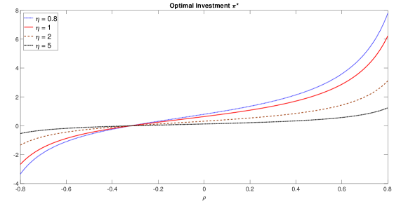
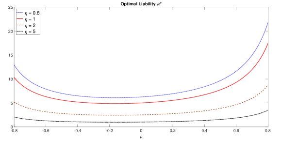
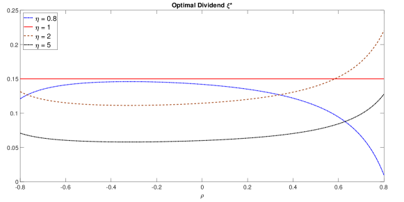
Figure 1: Impact of the Correlation Coefficient $\rho$ and Risk Aversion $\eta$ on the Optimal Strategies

Note. We plot the insurer’s optimal investment $\pi^{*}$ (upper panel), liability $\kappa^{*}$ (middle panel), and dividend $\xi^{*}$ (lower), as a function of the correlation coefficient $\rho$ over $(-0.8,0.8)$, under four different risk aversion levels $\eta=0.8$ (dotted blue), $\eta=1$ (solid red), $\eta=2$ (dashed brown), and $\eta=5$ (dash-dot black). The parameters are chosen from Table 1.

Our sensitivity analysis so far is based on the assumption that there are no jumps in the risk process $R$ (2.2). In what follows, we relax this assumption and numerically study how the jump intensity $\lambda$ affects the insurer’s optimal strategy $u^{*}$, which is now given by (3.12) in Proposition 3.2. Due to the inclusion of jumps, we now set the premium rate by the expected value principle: $p=(1+\theta)\times(\alpha+\lambda\gamma)$, where $\theta=50\%$. We further assume the insurer’s risk aversion is $\eta=2>1$ and fix the jump size $\gamma=0.3$ (3 times the diffusion parameter $\beta=0.1$). We plot the insurer’s optimal investment $\pi^{*}$, liability ratio $\kappa^{*}$, and dividend rate $\xi^{*}$ as a function of $\lambda$ over $(0.01,0.2)$ in Figure 2. The key results are summarized as follows:

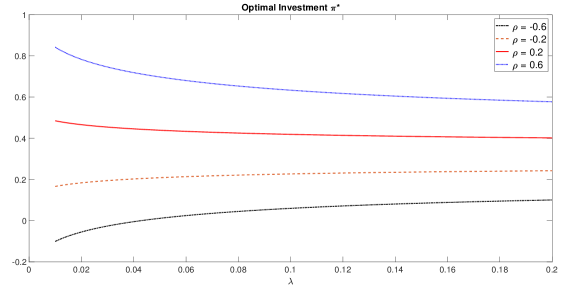
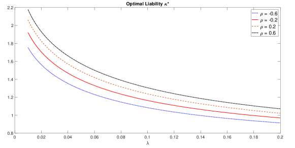
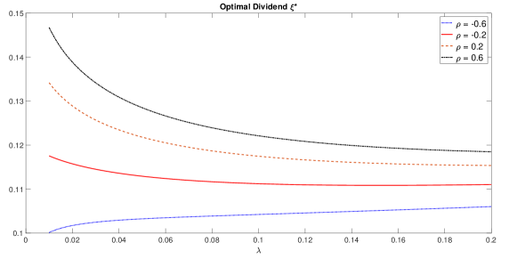
Figure 2: Impact of the Jump Intensity $\lambda$ on the Optimal Strategies

Note. We plot the insurer’s optimal investment $\pi^{*}$ (upper panel), liability $\kappa^{*}$ (middle panel), and dividend $\xi^{*}$ (lower), as a function of the jump intensity $\lambda$ over $(0.01,0.2)$, under four different correlation levels $\rho=-0.6$ (dotted blue), $\rho=-0.2$ (solid red), $\rho=0.2$ (dashed brown), and $\rho=0.6$ (dash-dot black). We set $p=1.5(\alpha+\lambda\gamma)$, $\eta=2$, $\gamma=0.3$, and the rest by Table 1.

• (Optimal investment $\pi^{*}$ in the upper panel of Figure 2)

  As anticipated, the results are divided into two regions of the correlation coefficient $\rho$ by a negative threshold $\hat{\rho}$. When $\rho$ is greater than $\hat{\rho}$, the optimal investment strategy $\pi^{*}$ is a decreasing function of the jump intensity $\lambda$, and thus the insurer invests less in the risky asset as $\lambda$ increases. When $\rho$ is less than $\hat{\rho}$, $\pi^{*}$ becomes an increasing function of $\lambda$. In particular, for a very negative $\rho$ (e.g., $\rho=-0.6$ in Figure 2), $\pi^{*}$ may even change from a negative value to a positive value when $\lambda$ increases. These results can be explained by the expression of $\pi^{*}$ in (3.12), which has a positive myopic term, independent of $\lambda$, and a hedging term with the same sign as $\rho$, which depends on $\lambda$ through $\kappa^{*}$. Last, Figure 2 also confirms the finding from Figure 1 that $\pi^{*}$ is an increasing function of $\rho$.

• (Optimal liability ratio $\kappa^{*}$ in the middle panel of Figure 2)

  We observe that $\kappa^{*}$ is a decreasing function of $\lambda$. The economic explanation for such a result is that, as $\lambda$ increases, the insurable risk becomes more risky, and the insurer’s rational response is to reduce underwriting. Another observation from the numerical example is that $\kappa^{*}$ increases as the correlation $\rho$ increases.

• (Optimal dividend rate $\xi^{*}$ in the bottom panel of Figure 2)

  Similar to the result of $\pi^{*}$, how the jump intensity $\lambda$ affects the optimal dividend strategy $\xi^{*}$ also depends on the value of $\rho$. When $\rho$ is greater than a negative threshold $\hat{\rho}$, a negative relation between $\xi^{*}$ and $\lambda$ is shown by Figure 2. However, for a very negative $\rho$ (e.g., $\rho=-0.6$ in Figure 2), it is possible that $\xi^{*}$ goes up as $\lambda$ increases. Following the discussions on $\rho$ in Section 5.1, let us interpret $\rho>\hat{\rho}$ as a “preferable” market condition and $\rho<\hat{\rho}$ an “adverse” market condition. In a preferable market, although an increase in $\lambda$ makes the insurance business more risky, the insurer still wants to maintain the surplus at a relatively high level (since the market is preferable), and to achieve so, the insurer reduces the optimal dividend rate. On the contrary, in an adverse market, the insurer pays dividend at a higher rate when $\lambda$ increases, that is because keeping a large surplus is no longer attractive when the available business opportunities are unfavorable. In other words, when the market is in adverse condition, the “utility” of cashing out dividends now outweighs the “utility” of saving for business opportunities in future.

6 Conclusions

We introduce a combined financial and insurance market consisting of a risk-free asset, a risky asset, and a risk process $R$. The risk process $R$ is modeled by a jump-diffusion process, possibly correlated with the risky asset, and represents the amount of liabilities per policy or per unit in underwriting. A representative insurer controls simultaneously the investment weight in the risky asset, the liability ratio in underwriting, and the dividend payout rate to shareholders. The insurer seeks an optimal triplet strategy to maximize her expected discounted utility of dividend over an infinite horizon. We first solve such an optimal dividend problem for constant strategies and then apply a perturbation approach to show that the optimal constant strategy remains optimal over all admissible strategies. When the insurer’s utility is given by a log or a power utility function, we obtain the optimal strategy and the value function in closed form. We further utilize the explicit results to conduct economic analyses, both analytically and numerically, to study the impact of various market parameters and risk aversion on the insurer’s optimal strategy.

Disclosure statement

No potential conflict of interest was reported by the author(s).

References

- Albrecher et al., (2005) Albrecher, H., Hartinger, J., and Tichy, R. F. (2005). On the distribution of dividend payments and the discounted penalty function in a risk model with linear dividend barrier. Scandinavian Actuarial Journal, 2005(2):103–126.
- Albrecher and Ivanovs, (2018) Albrecher, H. and Ivanovs, J. (2018). On the distribution of dividend payments and the discounted penalty function in a risk model with linear dividend barrier. Scandinavian Actuarial Journal, 2018(1):76–83.
- Albrecher and Thonhauser, (2009) Albrecher, H. and Thonhauser, S. (2009). Optimality results for dividend problems in insurance. RACSAM-Revista de la Real Academia de Ciencias Exactas, Físicas y Naturales. Serie A. Matemáticas, 103(2):295–320.
- Asmussen et al., (2000) Asmussen, S., Højgaard, B., and Taksar, M. (2000). Optimal risk control and dividend distribution policies. example of excess-of loss reinsurance for an insurance corporation. Finance and Stochastics, 4(3):299–324.
- Asmussen and Taksar, (1997) Asmussen, S. and Taksar, M. (1997). Controlled diffusion models for optimal dividend pay-out. Insurance: Mathematics and Economics, 20(1):1–15.
- Avanzi, (2009) Avanzi, B. (2009). Strategies for dividend distribution: A review. North American Actuarial Journal, 13(2):217–251.
- Avanzi and Gerber, (2008) Avanzi, B. and Gerber, H. U. (2008). Optimal dividends in the dual model with diffusion. ASTIN Bulletin, 38(2):653–667.
- Avanzi et al., (2007) Avanzi, B., Gerber, H. U., and Shiu, E. S. (2007). Optimal dividends in the dual model. Insurance: Mathematics and Economics, 41(1):111–123.
- Avanzi and Wong, (2012) Avanzi, B. and Wong, B. (2012). On a mean reverting dividend strategy with brownian motion. Insurance: Mathematics and Economics, 51(2):229–238.
- Azcue and Muler, (2005) Azcue, P. and Muler, N. (2005). Optimal reinsurance and dividend distribution policies in the Cramér-Lundberg model. Mathematical Finance, 15(2):261–308.
- Bai and Guo, (2010) Bai, L. and Guo, J. (2010). Optimal dividend payments in the classical risk model when payments are subject to both transaction costs and taxes. Scandinavian Actuarial Journal, 2010(1):36–55.
- Bayraktar et al., (2013) Bayraktar, E., Kyprianou, A. E., and Yamazaki, K. (2013). On optimal dividends in the dual model. ASTIN Bulletin, 43(3):359–372.
- Bayraktar et al., (2014) Bayraktar, E., Kyprianou, A. E., and Yamazaki, K. (2014). Optimal dividends in the dual model under transaction costs. Insurance: Mathematics and Economics, 54:133–143.
- Bernard et al., (2020) Bernard, C., Liu, F., and Vanduffel, S. (2020). Optimal insurance in the presence of multiple policyholders. Journal of Economic Behavior & Organization, forthcoming.
- Browne, (1995) Browne, S. (1995). Optimal investment policies for a firm with a random risk process: Exponential utility and minimizing the probability of ruin. Mathematics of Operations Research, 20(4):937–958.
- Cadenillas et al., (2006) Cadenillas, A., Choulli, T., Taksar, M., and Zhang, L. (2006). Classical and impulse stochastic control for the optimization of the dividend and risk policies of an insurance firm. Mathematical Finance, 16(1):181–202.
- Cadenillas et al., (2007) Cadenillas, A., Sarkar, S., and Zapatero, F. (2007). Optimal dividend policy with mean-reverting cash reservoir. Mathematical Finance, 17(1):81–109.
- Capponi and Figueroa-López, (2014) Capponi, A. and Figueroa-López, J. E. (2014). Dynamic portfolio optimization with a defaultable security and regime-switching. Mathematical Finance, 24(2):207–249.
- Chen et al., (2014) Chen, S., Li, Z., and Zeng, Y. (2014). Optimal dividend strategies with time-inconsistent preferences. Journal of Economic Dynamics and Control, 46:150–172.
- Choulli et al., (2003) Choulli, T., Taksar, M., and Zhou, X. Y. (2003). A diffusion model for optimal dividend distribution for a company with constraints on risk control. SIAM Journal on Control and Optimization, 41(6):1946–1979.
- De Finetti, (1957) De Finetti, B. (1957). Su un’impostazione alternativa della teoria collettiva del rischio. In Transactions of the XVth International Congress of Actuaries, volume 2, pages 433–443. New York.
- Fleming and Soner, (2006) Fleming, W. H. and Soner, H. M. (2006). Controlled Markov Processes and Viscosity Solutions. Springer Science & Business Media.
- Gerber and Shiu, (2004) Gerber, H. U. and Shiu, E. S. (2004). Optimal dividends: analysis with brownian motion. North American Actuarial Journal, 8(1):1–20.
- Grandits et al., (2007) Grandits, P., Hubalek, F., Schachermayer, W., and Žigo, M. (2007). Optimal expected exponential utility of dividend payments in a brownian risk model. Scandinavian Actuarial Journal, 2007(2):73–107.
- Gu et al., (2018) Gu, J.-W., Steffensen, M., and Zheng, H. (2018). Optimal dividend strategies of two collaborating businesses in the diffusion approximation model. Mathematics of Operations Research, 43(2):377–398.
- Herdegen et al., (2020) Herdegen, M., Hobson, D., and Jerome, J. (2020). An elementary approach to the merton problem. arXiv preprint arXiv:2006.05260.
- Højgaard and Taksar, (1998) Højgaard, B. and Taksar, M. (1998). Optimal proportional reinsurance policies for diffusion models. Scandinavian Actuarial Journal, 1998(2):166–180.
- Højgaard and Taksar, (1999) Højgaard, B. and Taksar, M. (1999). Controlling risk exposure and dividends payout schemes: insurance company example. Mathematical Finance, 9(2):153–182.
- Jeanblanc-Picqué and Shiryaev, (1995) Jeanblanc-Picqué, M. and Shiryaev, A. N. (1995). Optimization of the flow of dividends. Uspekhi Matematicheskikh Nauk, 50(2):25–46.
- Jin et al., (2020) Jin, Z., Liao, H., Yang, Y., and Yu, X. (2020). Optimal dividend strategy for an insurance group with contagious default risk. Scandinavian Actuarial Journal, forthcoming.
- Jin et al., (2013) Jin, Z., Yang, H., and Yin, G. (2013). Numerical methods for optimal dividend payment and investment strategies of regime-switching jump diffusion models with capital injections. Automatica, 49(8):2317–2329.
- Jin et al., (2015) Jin, Z., Yang, H., and Yin, G. (2015). Optimal debt ratio and dividend payment strategies with reinsurance. Insurance: Mathematics and Economics, 64:351–363.
- Karatzas et al., (1986) Karatzas, I., Lehoczky, J. P., Sethi, S. P., and Shreve, S. E. (1986). Explicit solution of a general consumption/investment problem. Mathematics of Operations Research, 11(2):261–294.
- Karatzas and Shreve, (1998) Karatzas, I. and Shreve, S. E. (1998). Methods of Mathematical Finance. Springer.
- Kulenko and Schmidli, (2008) Kulenko, N. and Schmidli, H. (2008). Optimal dividend strategies in a cramér–lundberg model with capital injections. Insurance: Mathematics and Economics, 43(2):270–278.
- Lapham et al., (1996) Lapham, E. V., Kozma, C., and Weiss, J. O. (1996). Genetic discrimination: Perspectives of consumers. Science, 274(5287):621–624.
- Lindensjö and Lindskog, (2020) Lindensjö, K. and Lindskog, F. (2020). Optimal dividends and capital injection under dividend restrictions. Mathematical Methods of Operations Research, pages 1–27.
- Merton, (1969) Merton, R. C. (1969). Lifetime portfolio selection under uncertainty: The continuous-time case. Review of Economics and Statistics, 51(3):247–257.
- Merton, (1971) Merton, R. C. (1971). Optimum consumption and portfolio rules in a continuous-time model. Journal of Economic Theory, 3(4):373–413.
- Meyer and Meyer, (2005) Meyer, D. J. and Meyer, J. (2005). Relative risk aversion: What do we know? Journal of Risk and Uncertainty, 31(3):243–262.
- Øksendal and Sulem, (2005) Øksendal, B. K. and Sulem, A. (2005). Applied Stochastic Control of Jump Diffusions. Springer.
- Schmidli, (2007) Schmidli, H. (2007). Stochastic Control in Insurance. Springer Science & Business Media.
- Schmidli, (2017) Schmidli, H. (2017). On capital injections and dividends with tax in a diffusion approximation. Scandinavian Actuarial Journal, 2017(9):751–760.
- Shen and Zou, (2021) Shen, Y. and Zou, B. (2021). Mean-varince investment and risk control strategies: A time-consistant approach via a forward anxiliary process. Insurance: Mathematics and Economics, 97:68–80.
- Sotomayor and Cadenillas, (2011) Sotomayor, L. R. and Cadenillas, A. (2011). Classical and singular stochastic control for the optimal dividend policy when there is regime switching. Insurance: Mathematics and Economics, 48(3):344–354.
- Stein, (2012) Stein, J. L. (2012). Stochastic Optimal Control and the US Financial Debt Crisis. Springer.
- Taksar and Zhou, (1998) Taksar, M. I. and Zhou, X. Y. (1998). Optimal risk and dividend control for a company with a debt liability. Insurance: Mathematics and Economics, 22(1):105–122.
- Thonhauser and Albrecher, (2007) Thonhauser, S. and Albrecher, H. (2007). Dividend maximization under consideration of the time value of ruin. Insurance: Mathematics and Economics, 41(1):163–184.
- Thonhauser and Albrecher, (2011) Thonhauser, S. and Albrecher, H. (2011). Optimal dividend strategies for a compound poisson process under transaction costs and power utility. Stochastic Models, 27(1):120–140.
- Xu et al., (2020) Xu, L., Yao, D., and Cheng, G. (2020). Optimal investment and dividend for an insurer under a markov regime switching market with high gain tax. Journal of Industrial & Management Optimization, 16(1):325.
- Yao et al., (2011) Yao, D., Yang, H., and Wang, R. (2011). Optimal dividend and capital injection problem in the dual model with proportional and fixed transaction costs. European Journal of Operational Research, 211(3):568–576.
- Zhou and Jin, (2020) Zhou, Z. and Jin, Z. (2020). Optimal equilibrium barrier strategies for time-inconsistent dividend problems in discrete time. Insurance: Mathematics and Economics, 94:100–108.
- Zhu, (2013) Zhu, J. (2013). Optimal dividend control for a generalized risk model with investment incomes and debit interest. Scandinavian Actuarial Journal, 2013(2):140–162.
- Zhu, (2015) Zhu, J. (2015). Dividend optimization for general diffusions with restricted dividend payment rates. Scandinavian Actuarial Journal, 2015(7):592–615.
- Zhu et al., (2020) Zhu, J., Siu, T. K., and Yang, H. (2020). Singular dividend optimization for a linear diffusion model with time-inconsistent preferences. European Journal of Operational Research, 285(1):66–80.
- Zou and Cadenillas, (2014) Zou, B. and Cadenillas, A. (2014). Optimal investment and risk control policies for an insurer: Expected utility maximization. Insurance: Mathematics and Economics, 58:57–67.