Flow-plane decorrelations in heavy-ion collisions with multiple-plane cumulants

Abstract

The azimuthal correlations between local flow planes at different (pseudo)rapidities ($\eta$) may reveal important details of the initial nuclear matter density distributions in heavy-ion collisions. Extensive experimental measurements of a factorization ratio ($r_{2}$) and its derivative ($F_{2}$) have shown evidence of the longitudinal flow-plane decorrelation. However, nonflow effects also affect this observable and prevent a quantitative understanding of the phenomenon. In this paper, to distinguish decorrelation and nonflow effects, we propose a new cumulant observable, $T_{2}$, which largely suppresses nonflow. The technique sensitivity to different initial-state scenarios and nonflow effects are tested with a simple Monte Carlo model, and in the end, the method is applied to events simulated by a multiphase transport model (AMPT) for Au+Au collisions at $\sqrt{s_{\rm NN}}=200$ GeV. We also emphasize that a distinct decorrelation signal requires not only the right sign of an observable, but also its proper dependence on the $\eta$-window of the reference flow plane, to be consistent with the pertinent decorrelation picture.

keywords

flow decorrelation, nonflow

I Introduction

Experiments on high-energy heavy-ion collisions, such as those at the BNL Relativistic Heavy Ion Collider (RHIC) and the CERN Large Hadron Collider (LHC), aim to create a quark gluon plasma (QGP) and to study the properties of this deconfined nuclear medium. Most heavy-ion collisions are not head-on, and traditionally, the nucleons experiencing at least one collision are considered as participants, and the remaining are labeled as spectators (see Fig. 1). While spectators fly away, the system created by the participant interaction presumably undergoes a hydrodynamic expansion. The initial geometry of the system is determined by the participant distribution, with event-by-event fluctuations. The pressure gradients of the medium convert the spatial anisotropies of the initial matter distribution into the momentum anisotropies of the final-state particles. Consequently, the azimuthal distributions of emitted particles can be analyzed with a Fourier expansion [1, 2]

$$\frac{dN}{d\varphi}\propto 1+\sum_{n=1}^{\infty}2v_{n}\cos[n(\varphi-\Psi^{\rm RP})],$$ (1)

where $\varphi$ denotes the azimuthal angle of a particle and $\Psi^{\rm RP}$ is the reaction plane azimuth (defined by the impact parameter vector). The Fourier coefficients,

$$v_{n}=\langle\cos[n(\varphi-\Psi^{\rm RP})]\rangle\,,$$ (2)

are referred to as anisotropic flow of the $n^{\rm th}$ harmonic. By convention, $v_{1}$, $v_{2}$ and $v_{3}$ are called “directed flow”, “elliptic flow”, and “triangular flow”, respectively. They reflect the hydrodynamic response of the system to the initial geometry (and its fluctuations) of the participant zone [3].

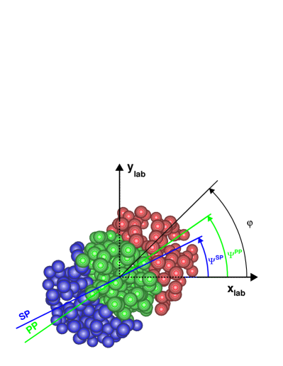
Figure 1: (Color online) Schematic view of a two-nucleus collision in the transverse plane. The left nucleus is emerging from and the right one going into the page. Particles are produced in the overlap region (green-colored are the participant nucleons). The azimuthal angles of the spectator plane ($\Psi^{\rm SP}$), the participant plane ($\Psi^{\rm PP}$) and one of the produced particles ($\varphi$) are depicted here.

In reality, the reaction plane is unknown, and more importantly, the initial-state fluctuations drive the anisotropic flow along the planes that differ from the reaction plane, the so-called flow symmetry planes or participant planes ($\Psi_{n}^{\rm PP}$). Then the particle azimuthal distributions can be rewritten as

$$\frac{dN}{d\varphi}\propto 1+\sum_{n=1}^{\infty}2v_{n}\cos[n(\varphi-\Psi_{n}^{\rm PP})].$$ (3)

The meaning of the flow coefficients $v_{n}$ changes from those in Eq. 2, but for simplicity of notations, the same symbols will be used, since in later discussions we will not determine the flow coefficients with the reaction plane. Anisotropic flow measurements relative to the participant plane are straightforward, as the flow itself can be used to estimate the corresponding flow plane. However, using the participant/flow plane also has its drawback – these planes become dependent on the kinematic region (rapidity and transverse momentum) of particles involved. This dependence is relatively weak, which still justifies the flow formalism of Eq. 3, but it needs to be taken into account to interpret high-precision flow measurements in modern experiments, especially the flow-plane decorrelation analyses to be discussed.

For clarity, we collect the definitions of different planes used in this paper below:

• Reaction plane (RP) is the plane spanned by the beam direction and the impact parameter vector. This plane is unique for every collision.

• Participant plane (PP) is defined by the initial density distribution. Subtle differences may exist, depending on, e.g., whether entropy or energy density is used as a weight, but these potentially small differences are not discussed in this paper. We assume that the properly constructed PPs define the development of anisotropic flow.

• Flow symmetry plane or flow plane (FP) determines the orientation of the corresponding harmonic anisotropic flow. It is assumed that FP coincides with the PP of the same harmonic (linear flow mode) or a proper combination of the lower harmonic PPs (nonlinear flow mode). With the nonlinear flow modes neglected, FP and PP are often used interchangeably.

• Event plane (EP) estimates the FP by analyzing the particle azimuthal distribution in a particular kinematic region. Owing to the finite number of particles involved in such an estimate, EP is subject to statistical fluctuations. The measurements obtained with EP have to be corrected for the event plane resolution [2], characterized by $\langle\cos[n(\Psi_{n}^{\rm EP}-\Psi_{n}^{\rm FP})]\rangle$. $\Psi^{\rm EP}$ is the azimuthal angle of the reconstructed $n^{\rm th}$-harmonic flow vector, ${\bf Q}_{n}=(\sum_{i}^{N}w_{i}\cos(n\varphi_{i}),\sum_{i}^{N}w_{i}\sin(n\varphi_{i}))$, where $w_{i}$ is the weight for each particle. For simplicity, we use unity weights in the event plane calculation.

• Spectator planes (SP) is determined by a sideward deflection of spectator nucleons, and is regarded as a better proxy for RP than FPs (determined by participants).

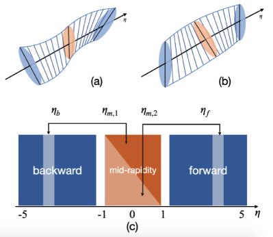
Figure 2: (Color online) Schematic view of (a) the “torque” or S-shaped , and (b) the bow or C-shaped decorrelation patterns in the longitudinal distribution of the flow plane angle. The ellipses indicate the transverse momentum distributions of the final-state particles. Panel (c) delimits the kinematic regions for the particles at mid-, forward, and backward pseudorapidities.

The objective of this paper is the flow-plane decorrelation in the (pseudo)rapidity ($\eta$) direction. Decorrelation here means the deviation of a local flow plane from the value at the center-of-mass rapidity ($y_{\rm CM}$), $\Delta\Psi(\eta)=\Psi(\eta)-\Psi(y_{\rm CM})$. For simplicity, $y_{\rm CM}$ is set to zero for the symmetric collisions under study. In practice, we measure the relative tilt angles between the flow planes at backward, mid-, and forward rapidities. For concreteness we focus on the $2^{\rm nd}$-harmonic flow. From event to event, two possible patterns arise from flow fluctuations: (a) when the flow plane angles at forward and backward pseudorapidities ($\Psi_{\rm f}$ and $\Psi_{\rm b}$) fall on the opposite sides of the flow plane at midrapidities ($\Psi_{\rm m}$) – the “torque” scenario, or S-shaped decorrelations, and (b) when $\Psi_{\rm f}$ and $\Psi_{\rm b}$ fall on the same side relative to $\Psi_{\rm m}$ – the “bow” scenario, or C-shaped decorrelations. These two cases are exemplified in panels (a) and (b) of Fig. 2, respectively.

The magnitude and pattern of the flow-plane decorrelation is extremely important, not only for the flow measurements (to be discussed in Sec. II), but also for understanding of the initial condition in the longitudinal direction. Flow-plane decorrelations can be caused by the torque effect [4], and more generally eccentricity decorrelations [5]. The mechanisms leading to the decorrelations also include hydrodynamic fluctuations in the QGP fluid [6] and glasma dynamics [7]. There also exists a phenomenological dynamical model of the initial states [8] that predicts the torque. We cannot exclude the possibility that the mechanisms causing the S-shaped decorrelations coexist with those originating the C-shaped ones in heavy-ion collisions. Therefore, experimental observables are only expected to measure the average effect and reveal the dominant decorrelation pattern.

A widely used measure of the longitudinal flow-plane decorrelation was introduced by the CMS Collaboration [9]:

$$r_{n}(\eta) = \frac{\langle\cos[n(\varphi_{-\eta}-\Psi_{\rm f})]\rangle}{\langle\cos[n(\varphi_{\eta}-\Psi_{\rm f})]\rangle}$$ (4)

$$= \frac{\langle v_{n}(-\eta)\cos[n(\Psi_{-\eta}-\Psi_{\rm f})]\rangle}{\langle v_{n}(\eta)\cos[n(\Psi_{\eta}-\Psi_{\rm f})]\rangle},$$ (5)

with $\eta>0$. $\Psi_{\rm f}$ can be replaced with $\Psi_{\rm b}$, if $\eta$ and $-\eta$ are simultaneously swapped in the definition. In a symmetric collision without any decorrelation, one would expect that $v(\eta)=v(-\eta)$ and the ratio to be unity. But if a torque pattern is present, with $\Psi_{\rm f}$ serving as a reference point, the decorrelation effect would be stronger for the negative-rapidity region, and the ratio would go below unity. Experimental data show that the factorization ratio $r_{2}$ indeed decreases with increasing $\eta$, and the deviation from unity is typically a few percent per unit pseudorapidity at both the LHC [9, 10, 11] and the RHIC [12]. Since both the flow-plane decorrelation and the flow-magnitude decorrelation can cause such a dependence of $r_{2}$ on $\eta$, efforts have been made to separate the two contributions [10, 13, 14]. However, before relating the observed $r_{2}(\eta)$ dependence to the flow-plane decorrelation, one has to examine an important physics background, the nonflow.

The nonflow effects are the correlations unrelated to the flow plane orientation or the initial geometry. Some nonflow effects are short-range in pseudorapidity, such as Coulomb and Bose-Einstein correlations (a few tenths of the unit of rapidity), resonance decays, and intra-jet correlations (about 1 unit rapidity), whereas back-to-back jets could contribute to the long-range correlations spanning over several units of rapidity. Therefore, even with a sizable $\eta$ gap between an event plane and the particles of interest, one can not completely eliminate nonflow contributions to $v_{2}$ or $r_{2}$ measurements. Nonetheless, the numerator of $r_{2}$ does involve a larger $\eta$ gap and hence a smaller nonflow contribution than its denominator, leading to a ratio smaller than unity, similar to that caused by the S-shaped flow-plane decorrelation. On the other hand, the C-shaped decorrelation may also be faked in experimental observables by nonflow effects such as back-to-back jet correlations.

In general, the decorrelation observables also depend on the $\eta$-window of the reference flow plane. In the following sections, we examine this dependence for various observables in the presence of nonflow and different types of flow-plane decorrelations. In Sec II, we use simple Monte Carlo simulations to demonstrate the impact of flow-plane decorrelations and nonflow on the $v_{2}$ measurements. Section III discusses the $r_{2}$ (and the closely related $F_{2}$ observable) analyses, and illustrates the possibilities of the $\eta$-differential measurements for a better interpretation of the results. We show that nonflow effects tend to cause overestimation of $F_{2}$, and to distort the $|\eta_{\rm f(b)}|$-dependence originally created by the flow-plane decorrelations. In Sec IV, we introduce a new four-plane observable, $T_{2}$, which is essentially free from the nonflow contribution and has very distinct expectations for different decorrelation patterns. In Sec V, the developed techniques are applied to the Au+Au events generated by a multiphase transport (AMPT) model [15]. Finally in Sec VI, we summarize the findings and discuss the application of the new method to experimental data.

II $v_{2}$ Monte-Carlo simulations

In elliptic flow measurements, it is a common practice to introduce a sizeable $\eta$ gap between the event plane ($\Psi_{\rm f(b)}$) and the particles of interest ($\varphi_{\rm m}$) to suppress nonflow:

$$v_{2}\{\Psi_{\rm f(b)}\}=\frac{\langle\cos[2(\varphi_{\rm m}-\Psi_{\rm f(b)})]\rangle}{\sqrt{\langle\cos[2(\Psi_{\rm f}-\Psi_{\rm b})]\rangle}},$$ (6)

where the denominator is the event plane resolution for $\Psi_{\rm f(b)}$. Although both the numerator and the denominator are contaminated by nonflow, the latter is less affected because of a larger $\eta$ gap between $\Psi_{\rm f}$ and $\Psi_{\rm b}$. Therefore the effect of nonlow on $v_{2}\{\Psi_{\rm f(b)}\}$ decreases with increasing the $\eta$ gap or $|\eta_{\rm f(b)}|$.

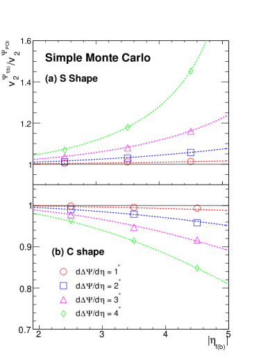
Figure 3: (Color online) Simple Monte Carlo calculations of the ratio, $v_{2}\{\Psi_{\rm f(b)}\}/v_{2}\{\Psi_{\rm POI}\}$, without nonflow for the S-shaped (a) and the C-shaped (b) flow-plane decorrelations as a function of $|\eta_{\rm f(b)}|$ and $\frac{d\Delta\Psi}{d\eta}$. The curves follow Eqs. (9) and (10).

When the S-shaped flow-plane decorrelation is present, both the numerator and the denominator in Eq. 6 are reduced by the finite tilt angles due to the $\eta$ gaps, and the denominator is more influenced because it involves an $\eta$ gap larger than that of the numerator. Therefore, the S-shaped decorrelation tends to drive $v_{2}\{\Psi_{\rm f(b)}\}$ above $v_{2}\{\Psi_{\rm POI}\}$, where $\Psi_{\rm POI}$ is the event plane determined in the same $\eta$ region as the particles of interest (POI).

To test these speculations, we perform a simple Monte Carlo simulation, where the tilt angle, $\Delta\Psi(\eta)$, is a linear function of $\eta$, with a slope of $\frac{d\Delta\Psi}{d\eta}=1^{\circ}$, $2^{\circ}$, $3^{\circ}$ or $4^{\circ}$:

$$\Delta\Psi(\eta)\equiv\Psi(\eta)-\Psi(0)=\frac{d\Delta\Psi}{d\eta}\eta.$$ (7)

In our simulation (see Appendix A for details), each event has 1000 particles, distributed uniformly in the $\eta$ range of (-5, 5). The particle density $\frac{dN}{d\eta}|_{\eta=0}=100$ corresponds roughly to the 30–50% centrality range in Au+Au collisions at $\sqrt{s_{\rm NN}}=200$ GeV, or 50–70% Pb+Pb at $\sqrt{s_{\rm NN}}=2.76$ TeV. The azimuthal angle of each particle has been assigned randomly according to the distribution of Eq. 3, and $\Psi^{\rm PP}$ is replaced with $\Psi(\eta)$. The POIs are selected within $|\eta|<1$, and the $|\eta_{\rm f(b)}|$ ranges used for calculations of $\Psi_{\rm f}$ and $\Psi_{\rm b}$ are taken from three bins: (2, 3), (3, 4) and (4, 5). For simplicity, the input $v_{2}$ is independent of $\eta$ or transverse momentum ($p_{T}$), and the simulation does not include nonflow at this step. We implement a $15\%$ flow fluctuation in all the following simple simulations, and observe no difference from results with zero fluctuation. Figure 3(a) shows that the $v_{2}\{\Psi_{\rm f(b)}\}/v_{2}\{\Psi_{\rm POI}\}$ ratio is above unity, and increases with both $|\eta_{\rm f(b)}|$ and $\frac{d\Delta\Psi}{d\eta}$, as expected for the S-shaped decorrelations. In the case of the C-shaped decorrelations, similar to Eq. 7, we assume

$$\Delta\Psi(\eta)=\frac{d\Delta\Psi}{d\eta}|\eta|,$$ (8)

and still vary $\frac{d\Delta\Psi}{d\eta}$ from $1^{\circ}$ to $4^{\circ}$. Now that the tilt angle is symmetric around $\eta=0$, the denominator in Eq. 6 is unchanged, and $v_{2}\{\Psi_{\rm f(b)}\}$ tends to under-estimate $v_{2}\{\Psi_{\rm POI}\}$. Indeed, Fig. 3(b) shows that the $v_{2}\{\Psi_{\rm f(b)}\}/v_{2}\{\Psi_{\rm POI}\}$ ratio goes below unity, and decreases with increasing $|\eta_{\rm f(b)}|$ and $\frac{d\Delta\Psi}{d\eta}$ for the C-shaped case. The ratios for the S-shaped and C-shaped scenarios can be well described, respectively, by

$$\frac{v_{2}\{\Psi_{\rm f(b)}\}}{v_{2}\{\Psi_{\rm POI}\}} = \frac{\cos(2\frac{d\Delta\Psi}{d\eta}|\eta_{\rm f(b)}|)}{\sqrt{\cos(4\frac{d\Delta\Psi}{d\eta}|\eta_{\rm f(b)}|)}}{\rm~{}(S~{}shape)},$$ (9)

$$\frac{v_{2}\{\Psi_{\rm f(b)}\}}{v_{2}\{\Psi_{\rm POI}\}} = \cos[2\frac{d\Delta\Psi}{d\eta}(|\eta_{\rm f(b)}|-0.5)]{\rm~{}(C~{}shape)}.$$ (10)

Therefore, to manifest a clear decorrelation signal, the $v_{2}$ ratio should go above unity with a rising trend vs $|\eta_{\rm f(b)}|$ for a torque (S-shaped) case, or below unity with a falling trend for a bow (C-shaped) case.

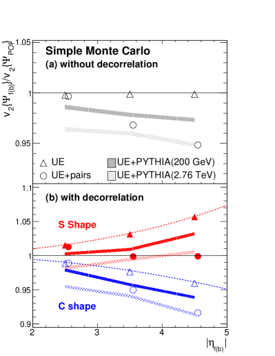
Figure 4: (Color online) Simple Monte Carlo calculations of the $v_{2}\{\Psi_{\rm f(b)}\}/v_{2}\{\Psi_{\rm POI}\}$ ratio as a function of $|\eta_{\rm f(b)}|$ for the underlying event (UE) without nonflow as well as for different scenarios of nonflow. $\frac{d\Delta\Psi}{d\eta}$ is set to $2^{\circ}$ for the S-shaped and the C-shaped flow-plane decorrelations. The curves follow Eqs. 9 and 10 without nonflow. The shaded bands represent the two cases of PYTHIA embedding.

We further implement nonflow correlations in the simulation, by adding to the “underlying” event (UE) pairs of particles with the same azimuthal angle. This nonflow simulation is similar to that used in Sec. IV(D) of Ref [16]. Note that since we deal with the $2^{\rm nd}$-harmonic flow, the near-side pairs with $\Delta\varphi\sim 0$ are equivalent to the away-side pairs with $\Delta\varphi\sim\pi$. One of the paired particles follows the uniform $\eta$ distribution within (-5, 5), and the other particle is separated with an $\eta$ gap that obeys a Gaussian distribution with a width of 2 units of pseudorapidity. Four hundred paired particles (200 pairs) have been added to each underlying event. The simulated $v_{2}\{\Psi_{\rm f(b)}\}/v_{2}\{\Psi_{\rm POI}\}$ ratio is shown in Fig. 4 as a function of $|\eta_{\rm f(b)}|$ with different amounts of nonflow. Panel (a) displays the scenario without any decorrelation, where nonflow fakes a falling trend. Panel (b) gives an example with $\frac{d\Delta\Psi}{d\eta}=2^{\circ}$ for the S-shaped and the C-shaped flow-plane decorrelations. In both scenarios, nonflow pulls down the original trends, and in the case of the S-shaped decorrelation, the initially rising trend could even be reversed into a falling one. Therefore, the $v_{2}\{\Psi_{\rm f(b)}\}/v_{2}\{\Psi_{\rm POI}\}$ ratio alone lacks discernment of different decorrelation scenarios.

Besides the simplified implementation of nonflow, which could exaggerate the effect, we also take a more realistic approach by embedding a few PYTHIA [17] events from p+p collisions at $\sqrt{s}=200$ GeV or $2.76$ TeV, such that PYTHIA particles replace the 400 paired particles (200 pairs). PYTHIA is an event generator that comprises a coherent set of physics mechanisms for the evolution from a few-body hard scattering process to a complex multihadronic final state. The corresponding results are shown with shaded bands in Fig. 4. The $v_{2}$ ratios thus obtained qualitatively show pull-down effects similar to the simplified nonflow case, with a stronger magnitude at the higher collision energy. In this study the embedding of PYTHIA particles into underlying events is done mostly to illustrate the effects of nonflow, but with parameters tuned to a specific centrality interval, it can also provide a quantitative estimate of nonflow contributions in the data analyses. More discussions on the simple Monte Carlo simulations and the nonflow effects can be found in Appendix A.

III $r_{2}$ and $F_{2}$

We define $r_{2}(\eta)$ based on Eq. 4 by setting $n=2$. As suggested by Eq. 5, the deviation of $r_{2}$ from unity may originate from the decorrelations both in the flow-plane angles and in the $v_{2}$ magnitudes. Thus, we also examine the modified observable, $r_{2}^{\Psi}$ [13], which is supposedly sensitive only to the flow-plane angles:

$$r_{2}^{\Psi}(\eta)=\frac{\langle\cos[2(\Psi_{-\eta}-\Psi_{\rm f})]\rangle}{\langle\cos[2(\Psi_{\eta}-\Psi_{\rm f})]\rangle}.$$ (11)

Experimentally as well as in model studies below, the dependence of $r_{2}^{(\Psi)}$ on $\eta$ is almost linear, and the $F_{2}^{(\Psi)}$ slope is used to quantify the effect [9]:

$$r_{2}^{(\Psi)}=1-2F_{2}^{(\Psi)}\eta.$$ (12)

We perform the linear-$\Delta\Psi(\eta)$ Monte Carlo simulation without nonflow to inspect the qualitative expectation of $F_{2}$ in the presence of the S-shaped flow-plane decorrelation. Note that in the C-shaped case, $F_{2}$ is zero by construction. In our simple simulations, $F_{2}$ and $F_{2}^{\Psi}$ are always identical, so only the $F_{2}$ results are presented. Figure 5 depicts $F_{2}$ as a function of $|\eta_{\rm f(b)}|$ and $\frac{d\Delta\Psi}{d\eta}$. $F_{2}$ increases with $\frac{d\Delta\Psi}{d\eta}$, since a larger tilt angle means a stronger torque. At first glance, it seems to be counter-intuitive that $F_{2}$ depends on the $\eta$ location of the reference event plane, but the simulation actually reveals a simple mathematical relation:

$$1-2F_{2}\eta=\frac{\cos[2(\eta+|\eta_{\rm f(b)}|)\frac{d\Delta\Psi}{d\eta}]}{\cos[2(\eta-|\eta_{\rm f(b)}|)\frac{d\Delta\Psi}{d\eta}]},$$ (13)

which yields $F_{2}\approx 4(d\Delta\Psi/d\eta)^{2}|\eta_{\rm f(b)}|$. Although in real collisions, the dependence of $\Delta\Psi$ on $\eta$ may not be linear, we have verified with various monotonic function forms that the larger the $\eta$ gap between POIs and the reference event plane is, the larger $F_{2}$ is. Thus an experimental observation of positive $F_{2}$ values with an increasing $F_{2}(|\eta_{\rm f(b)}|)$ trend may reveal a distinct domination of the S-shaped flow-plane decorrelations.

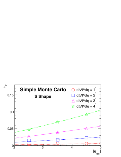
Figure 5: (Color online) $F_{2}$ as a function of $|\eta_{\rm f(b)}|$ and $\frac{d\Delta\Psi}{d\eta}$, from a simple Monte Carlo simulation for the S-shaped flow-plane decorrelation without nonflow. The curves reflect the analytical relation in Eq. 13.

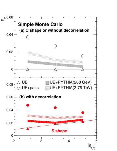
Figure 6: (Color online) Simple Monte Carlo calculations of $F_{2}(|\eta_{\rm f(b)}|)$ for the underlying event (UE) without nonflow as well as for different scenarios of nonflow. $\frac{d\Delta\Psi}{d\eta}$ is set to $2^{\circ}$ for the S-shaped and the C-shaped flow-plane decorrelations. The curve follows the ideal relation in Eq. 13 without nonflow. The shaded bands represent the two cases of PYTHIA embedding.

In Fig. 6, nonflow contributions have been studied under the same framework as that used for the $v_{2}\{\Psi_{\rm f(b)}\}/v_{2}\{\Psi_{\rm POI}\}$ ratio. Since the simple simulation results on $F_{2}$ are the same for the scenarios with no decorrelation and with the C-shaped decorrelation, we use one set of data points to present both of them in panel (a). In these two scenarios, nonflow can fake a finite $F_{2}$ value, which decreases with increasing $|\eta_{\rm f(b)}|$. Furthermore, panel (b) shows that nonflow not only quantitatively increases the magnitude of $F_{2}$ for the S-shaped decorrelation, but could also qualitatively change its rising trend into a falling one vs $|\eta_{\rm f(b)}|$. The embedding of 400 PYTHIA particles resembles the simplified nonflow implementation with weaker effects, but finite $F_{2}$ values are still faked when the truth is no decorrelation or the C-shaped decorrelation. For the S-shaped decorrelation, the rising trend vs $|\eta_{\rm f(b)}|$ is still distorted, especially at intermediate $|\eta_{\rm f(b)}|$. Therefore, $F_{2}$ cannot unambiguously distinguish and quantify different decorrelation scenarios. Figure 2(a) of Ref. [11] gives a concrete example of such nonflow effects on the $|\eta_{\rm f(b)}|$ dependence of $F_{2}$ in Xe+Xe collisions at $\sqrt{s_{\rm NN}}=5.44$ TeV.

IV $T_{2}$ analyses

In view of possible significant nonflow contributions in $v_{2}\{\Psi_{\rm f(b)}\}$ and $F_{2}$ analyses, we advocate a new observable to probe the longitudinal flow-plane decorrelation:

$$T_{2}=\frac{\langle\langle\sin 2(\Psi_{\rm f}-\Psi_{{\rm m},1})\sin 2(\Psi_{\rm b}-\Psi_{{\rm m},2})\rangle\rangle}{Res(\Psi_{\rm f})Res(\Psi_{{\rm m},1})Res(\Psi_{\rm b})Res(\Psi_{{\rm m},2})},$$ (14)

where particles at midrapidities ($|\eta|<1$) are divided into two sub-events to form $\Psi_{{\rm m},1}$ and $\Psi_{{\rm m},2}$, as demonstrated in Fig. 2(c). The double brackets denote “cumulant”, and operate as follows:

$$\langle\langle\sin(a-b)\sin(c-d)\rangle\rangle$$ (15)

$$\equiv \langle\sin(a-b)\sin(c-d)\rangle-\frac{1}{2}\langle\cos(a-c)\rangle\langle\cos(b-d)\rangle$$

$$+\frac{1}{2}\langle\cos(a-d)\rangle\langle\cos(b-c)\rangle,$$

the derivation of which is elaborated in Appendix B. Taking into account the flow fluctuation contributions in the event plane resolution, we have

$$T_{2} = \frac{\langle\sin 2(\Psi_{\rm f}-\Psi_{{\rm m},1})\sin 2(\Psi_{\rm b}-\Psi_{{\rm m},2})\rangle}{\langle\cos 2(\Psi_{\rm f}-\Psi_{{\rm m},1})\cos 2(\Psi_{\rm b}-\Psi_{{\rm m},2})\rangle}$$ (16)

$$- \frac{\langle\cos 2(\Psi_{\rm f}-\Psi_{\rm b})\rangle\langle\cos 2(\Psi_{{\rm m},1}-\Psi_{{\rm m},2})\rangle}{2\langle\cos 2(\Psi_{\rm f}-\Psi_{{\rm m},1})\rangle\langle\cos 2(\Psi_{\rm b}-\Psi_{{\rm m},2})\rangle}+\frac{1}{2}.$$

The generalization of the $T_{2}$ definition to four independent pseudorapidity ranges is straightforward and is discussed in Appendix C.

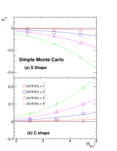
Figure 7: (Color online) Simple Monte Carlo simulations of $T_{2}$ as a function of $|\eta_{\rm f(b)}|$ and $\frac{d\Delta\Psi}{d\eta}$ for the S-shaped (a) and the C-shaped (b) flow-plane decorrelations without nonflow. The curves express Eqs. 17 and 18.

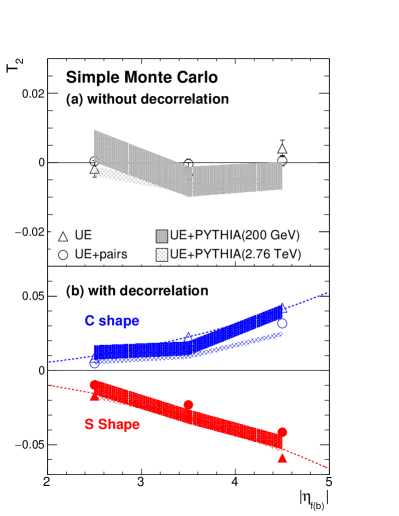
Figure 8: (Color online) Simple Monte Carlo calculations of $T_{2}$ as a function of $|\eta_{\rm f(b)}|$ for the underlying event (UE) without nonflow as well as for different scenarios of nonflow. $\frac{d\Delta\Psi}{d\eta}$ is set to $2^{\circ}$ for the S-shaped and the C-shaped flow-plane decorrelations. The curves manifest Eqs. 17 and 18 without nonflow. The shaded bands represent the two cases of PYTHIA embedding.

Defined as a four-particle cumulant, $T_{2}$ is essentially free from non-flow contribution (see Ref. [16] and references therein). $T_{2}$, as expressed in Eq. 14, provides an intuitive way to tell whether $\Psi_{\rm f}$ and $\Psi_{\rm b}$ fall on the same side or the opposite sides of $\Psi_{\rm m}$: a positive $T_{2}$ means a bow or a C-shaped decorrelation, and a negative $T_{2}$ signifies a torque or an S-shaped decorrelation. As done in the past, we shall exploit the linear-$\Delta\Psi(\eta)$ simulation without nonflow to learn the qualitative dependence of $T_{2}$ on $|\eta_{\rm f(b)}|$ and $\frac{d\Delta\Psi}{d\eta}$ in different decorrelation patterns. With a specific $\frac{d\Delta\Psi}{d\eta}$, Fig. 7 shows a rapid decreasing trend of $T_{2}$ vs $|\eta_{\rm f(b)}|$ for the S-shaped case in panel (a), and an increasing trend for the C-shaped case in panel (b). The simulated points obey the following mathematical relations:

$$T_{2} = -\frac{\sin^{2}(2\frac{d\Delta\Psi}{d\eta}|\eta_{\rm f(b)}|)+\frac{1}{2}\cos(4\frac{d\Delta\Psi}{d\eta}|\eta_{\rm f(b)}|)}{\cos^{2}(2\frac{d\Delta\Psi}{d\eta}|\eta_{\rm f(b)}|)}+\frac{1}{2}$$ (17)

$$= -\frac{1}{2}\tan^{2}(2\frac{d\Delta\Psi}{d\eta}|\eta_{\rm f(b)}|){\rm~{}(S~{}shape)},$$

$$T_{2} = \frac{\sin^{2}[2\frac{d\Delta\Psi}{d\eta}(|\eta_{\rm f(b)}|-0.5)]-\frac{1}{2}}{\cos^{2}[2\frac{d\Delta\Psi}{d\eta}(|\eta_{\rm f(b)}|-0.5)]}+\frac{1}{2}$$ (18)

$$= \frac{1}{2}\tan^{2}[2\frac{d\Delta\Psi}{d\eta}(|\eta_{\rm f(b)}|-0.5)]{\rm~{}(C~{}shape)}.$$

Again, in reality, the tilt angle may not increase linearly with the $\eta$ gap, but we have confirmed with various monotonic function forms that the falling and rising trends of $T_{2}$ vs $|\eta_{\rm f(b)}|$ should be solid expectations for the S-shaped and the C-shaped decorrelations, respectively.

In $v_{2}\{\Psi_{\rm f(b)}\}$ and $F_{2}$ analyses, the core element is a cosine function that yields large values close to 1 in strong-nonflow scenarios. Conversely, $T_{2}$ uses the cumulant of a sine function that gives close-to-zero nonflow contributions. Nonflow studies on $T_{2}$ are presented in Fig. 8 with the same procedure as before. Panel (a) shows that for the scenario without any decorrelation, the $T_{2}$ results are mostly consistent with zero, with a potential of slightly negative values with the embedding of PYTHIA events at 2.76 TeV. Panel (b) shows that for the scenarios with the C-shaped and the S-shaped decorrelations, the $T_{2}$ magnitude could be slightly reduced by nonflow, but the original trends are not changed vs $|\eta_{\rm f(b)}|$.

V AMPT studies

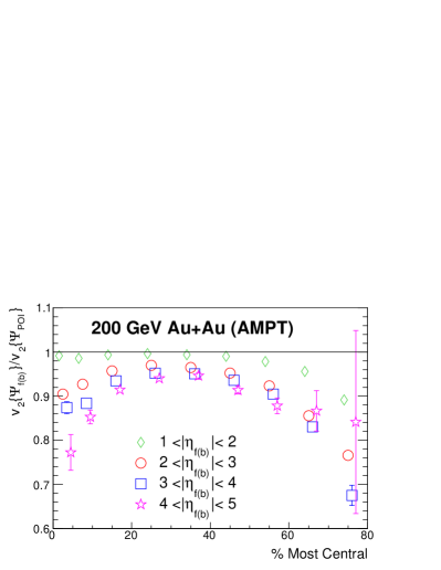
Figure 9: (Color online) AMPT calculations of the $|\eta_{\rm f(b)}|$ dependence of the $v_{2}\{\Psi_{\rm f(b)}\}/v_{2}\{\Psi_{\rm POI}\}$ ratio in different centrality intervals of Au+Au collisions at $\sqrt{s_{\rm NN}}=200$ GeV. Results using $\Psi_{\rm f}$ and $\Psi_{\rm b}$ are combined. Some points are staggered horizontally to improve visibility.

We test the aforementioned methodology with more realistic events, simulated by the AMPT model [15]. AMPT is a hybrid transport event generator, and describes four major stages of a high-energy heavy-ion collision: the initial conditions, the partonic evolution, the hadronization, and the hadronic interactions. For the initial conditions, AMPT uses the spatial and momentum distributions of minijet partons and excited soft strings, as adopted in the Heavy Ion Jet Interaction Generator (HIJING) [18]. Then Zhang’s parton cascade [19] is deployed to manage the partonic evolution, determined by the two-body parton-parton elastic scattering. At the end of the partonic evolution, the hadronization is implemented via the spatial quark coalescence. Finally, the hadronic interactions are modeled by a relativistic transport calculation [20]. The string-melting (SM) version of AMPT reasonably well reproduces particle spectra and elliptic flow in Au+Au collisions at $\sqrt{s_{\rm NN}}=200$ GeV and Pb+Pb collisions at 2.76 TeV [21]. In this study, Au+Au collisions at 200 GeV are simulated by the SM version v2.25t4cu of AMPT.

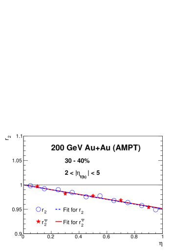
Figure 10: (Color online) $r_{2}(\eta)$ and $r_{2}^{\Psi}(\eta)$ in 30-40% Au+Au collisions at $\sqrt{s_{\rm NN}}=200$ GeV, simulated by AMPT. Results using $\Psi_{\rm f}$ and $\Psi_{\rm b}$ are combined. The straight-line fits to the $r_{2}$ and $r_{2}^{\Psi}$ points extract the corresponding $F_{2}$ of $(2.47\pm 0.11)\times 10^{-2}$ and $F_{2}^{\Psi}$ of ($2.43\pm 0.11)\times 10^{-2}$.

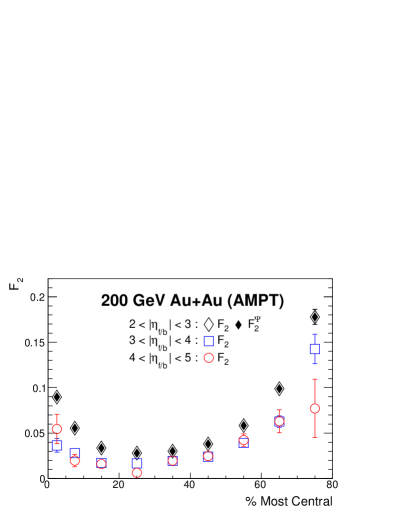
Figure 11: (Color online) $F_{2}$ and $F_{2}^{\Psi}$ for different $\eta_{\rm f/b}$ ranges as functions of centrality in Au+Au collisions at $\sqrt{s_{\rm NN}}=200$ GeV from AMPT.

In the following analyses of the AMPT events, we only select $\pi^{\pm}$, $K^{\pm}$, $p$ and $\bar{p}$ with $0.15<p_{T}<2$ GeV/$c$. $\varphi_{\rm m}$ and $\Psi_{\rm m}$ are delimited with $|\eta|<1$, and $\Psi_{\rm f}$ and $\Psi_{\rm b}$ are reconstructed with particles within $2<\eta<5$ and $-5<\eta<-2$, respectively. With the expectations from nonflow and the scenarios of flow-plane decorrelations in mind (see Figs. 3 and 4), we examine the $|\eta_{\rm f(b)}|$ dependence of the $v_{2}\{\Psi_{\rm f(b)}\}/v_{2}\{\Psi_{\rm POI}\}$ ratio in AMPT. Figure 9 shows the AMPT calculations of this ratio for four $|\eta_{\rm f(b)}|$ bins in different centrality intervals of Au+Au collisions at $\sqrt{s_{\rm NN}}=200$ GeV. Within each centrality bin, $v_{2}\{\Psi_{\rm f(b)}\}/v_{2}\{\Psi_{\rm POI}\}$ displays a decreasing trend with the increasing $\eta$ gap, excluding the S-shaped decorrelation from the dominant underlying mechanisms. Both nonflow and the C-shaped decorrelation could induce such a decreasing trend in the $v_{2}$ ratio, and we cannot yet discern the two scenarios using this observable.

Next, the AMPT results of $r_{2}(\eta)$ and $r_{2}^{\Psi}(\eta)$ are compared in Fig. 10 for 30-40% Au+Au collisions at 200 GeV. As mentioned earlier, $\Psi_{\rm f}$ can be replaced with $\Psi_{\rm b}$ in the $r_{2}$ definition, with $\eta$ and $-\eta$ simultaneously exchanged. The two sets of results have been combined to gain better statistics. Both $r_{2}$ and $r_{2}^{\Psi}$ show a linear trend decreasing as $\eta$ increases, seemingly indicating a torque in the flow-plane decorrelation at midrapidities. The linear fits render the very close values of $F_{2}=(2.47\pm 0.11)\times 10^{-2}$ and $F_{2}^{\Psi}=(2.43\pm 0.11)\times 10^{-2}$, which implies a marginal contribution of $v_{2}$-magnitude decorrelations at midrapidities in AMPT events.

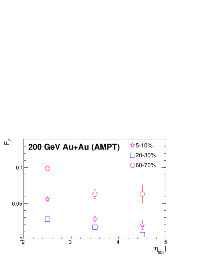
Figure 12: (Color online) AMPT calculations of $F_{2}$ versus $|\eta_{\rm f(b)}|$ for three selected centrality ranges in Au+Au collisions at $\sqrt{s_{\rm NN}}=200$ GeV.

Figure 11 presents the AMPT calculations of $F_{2}$ and $F_{2}^{\Psi}$ for different $\eta_{\rm f/b}$ ranges as a function of centrality. The two quantities are very close to each other in most centrality bins, and to avoid clutter, we only show $F_{2}^{\Psi}$ for the case of $2<|\eta_{\rm f/b}|<3$ as a demonstration. Thereafter, we focus on $F_{2}$. For the three $|\eta_{\rm f/b}|$ ranges, the magnitude of $F_{2}$ is about 2.5% in the 10–50% centrality range, and becomes larger in more central and more peripheral events. Before attributing the finite $F_{2}$ values to the flow-plane decorrelation, one should note that such a centrality dependence could be a reflection of nonflow effects. Nonflow contributions are positive in $F_{2}$, and become more pronounced in peripheral collisions where multiplicity is low and in central collisions where $v_{2}$ is small. This caveat also applies to experimental data [12, 9] that show $F_{2}$ features similar to these AMPT simulations. Moreover, the $F_{2}$ dependence on $|\eta_{\rm f/b}|$ and centrality qualitatively resembles Fig.2(a) of Ref. [11], corroborating the nonflow contribution.

The qualitative expectation from the simple Monte Carlo simulation (see Figs. 5 and 6) motivates the differential measurements of $F_{2}$ with respect to $|\eta_{\rm f(b)}|$. Figure 12 delineates AMPT calculations of $F_{2}$ as a function of $|\eta_{\rm f(b)}|$ for three selected centrality bins in Au+Au collisions at 200 GeV. The $F_{2}$ values are positive for all the cases under study, consistent with the S-shaped decorrelation. However, the $|\eta_{\rm f(b)}|$ dependence shows a falling trend in each centrality interval, in contrast to the rising trend expected for the torque alone. Therefore, the contribution of the S-shaped flow-plane decorrelation in these $F_{2}$ values, if any, must have been dominated by nonflow effects, which are also positive, and decrease with increasing $|\eta_{\rm f(b)}|$.

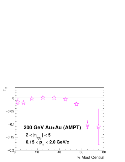
Figure 13: (Color online) Centrality dependence of $T_{2}$ in AMPT events of Au+Au collisions at $\sqrt{s_{\rm NN}}=200$ GeV. The $|\eta_{\rm f(b)}|$ range is (2, 5) for $\Psi_{\rm f}$ and $\Psi_{\rm b}$.

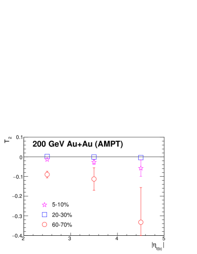
Figure 14: (Color online) $T_{2}$ dependence on $|\eta_{\rm f(b)}|$ for three selected centrality ranges in AMPT events of Au+Au at $\sqrt{s_{\rm NN}}=200$ GeV.

Finally, Fig. 13 depicts the $T_{2}$ values as a function of centrality in the AMPT events of Au+Au collisions at 200 GeV. For the 10–50% centrality range, $T_{2}$ is consistent with zero, indicating no apparent flow-plane decorrelation. In more central or more peripheral events, $T_{2}$ falls negative, supporting the picture of a torque or the S-shaped decorrelation. Note that when the tilt angle between $\Psi_{\rm m}$ and $\Psi_{\rm f(b)}$ becomes large, the denominator of $T_{2}$ significantly under-estimates the product of the event-plane resolutions, which in turn will blow up the magnitudes of both $T_{2}$ and its statistical uncertainty. This effect partially attributes to the large $T_{2}$ magnitudes and the large error bars in peripheral collisions. The bright side is that this effect does not change the sign of $T_{2}$, because the denominator is always positive by symmetry.

The AMPT results of $T_{2}$ as a function of $|\eta_{\rm f(b)}|$ are plotted in Fig. 14 for three selected centrality bins in Au+Au collisions at 200 GeV. For the 20–30% centrality range, $T_{2}$ is always consistent with zero, whereas for 5–10% and 60–70% collisions, there seem to be decreasing trends due to a torque, although the statistical uncertainties become large at increased $|\eta_{\rm f(b)}|$. Therefore, both the sign and the $|\eta_{\rm f(b)}|$-dependence of $T_{2}$ confirm the S-shaped longitudinal decorrelation in central and peripheral AMPT events.

A comparison between $F_{2}$ and $T_{2}$ is possible, if we neglect nonflow effects for the moment, and use Eqs. 13, 17 and 18 to extract the tilt angles from these two observables. Table I lists the values of $F_{2}$ and $T_{2}$ as a function of centrality for $2<|\eta_{\rm f(b)}|<5$ from Figs. 11 and 13, as well as the extracted tilt angles. The average $|\eta_{\rm f(b)}|$ is around 3.2 with a weak centrality dependence. In general, the tilt angles obtained from $F_{2}$ have magnitudes larger than those from $T_{2}$, and the difference could be attributed to contributions other than nonflow. The smaller tilt-angle values obtained from $T_{2}$ might also indicate a stochastic nature of the flow-plane decorrelations as a function of $\Delta\eta$. For example, one can model the flow-plane angle along the longitudinal direction with a Markov chain: the $\eta$ range is divided into many small steps, and the flow plane at each step is randomly tilted by a small amount with respect to that at the previous step. In that case $\langle(\Delta\Psi)^{2}\rangle\propto\Delta\eta$. Such a random-walk-like process will lead to a positive $F_{2}$ independent of $|\eta_{\rm f(b)}|$, but have zero contribution to $T_{2}$.

Table 1: AMPT results of $T_{2}$ and $F_{2}$ for $2<|\eta_{\rm f(b)}|<5$ from Figs. 11 and 13 as well as the corresponding tilt angles ($\frac{d\Delta\Psi}{d\eta}$) versus centrality in Au+Au collisions at 200 GeV. $\frac{d\Delta\Psi}{d\eta}$ is extracted using Eqs. 13, 17 and 18 without nonflow. For the tilt angles from $T_{2}$, a minus sign is added, if the decorrelation is C-shaped.

% central	$F_{2}$ (%)	$T_{2}$ (%)	$\frac{d\Delta\Psi}{d\eta}\{F_{2}\}$ (∘)	$\frac{d\Delta\Psi}{d\eta}\{T_{2}\}$ (∘)
0-5	7.0 (0.4)	-1.5 (1.1)	4.26 (0.13)	1.3 (0.9)
5-10	4.3 (0.2)	-1.8 (0.5)	3.37 (0.09)	1.7 (0.2)
10-20	2.6 (0.1)	-0.2 (0.2)	2.61 (0.06)	0.5 (0.4)
20-30	2.1 (0.1)	0.1 (0.2)	2.35 (0.06)	-0.4 (0.5)
30-40	2.6 (0.1)	0.1 (0.2)	2.57 (0.06)	-0.2 (0.6)
40-50	3.1 (0.1)	-0.5 (0.3)	2.84 (0.06)	0.8 (0.3)
50-60	4.9 (0.2)	-2.4 (0.6)	3.57 (0.08)	1.9 (0.2)
60-70	8.1 (0.4)	-10.2 (1.5)	4.58 (0.10)	3.8 (0.3)
70-80	16.0 (0.9)	-11.0 (6.8)	6.42 (0.17)	3.6 (1.7)

VI Conclusions

The flow-plane azimuthal decorrelations provide important input to the initial condition and the system evolution of heavy-ion collisions in the longitudinal dimension. We have explored three analyses that may be sensitive to such decorrelations: $v_{2}\{\Psi_{\rm f(b)}\}/v_{2}\{\Psi_{\rm POI}\}$, $F_{2}^{(\Psi)}$ and $T_{2}$. Using simple Monte Carlo simulations with a constant $\frac{d\Delta\Psi}{d\eta}$ slope, we have learned the impacts of decorrelation and nonflow on these observables as functions of $|\eta_{\rm f(b)}|$.

• In the absence of nonflow, the $v_{2}\{\Psi_{\rm f(b)}\}/v_{2}\{\Psi_{\rm POI}\}$ ratio will increase(decrease) with increasing $|\eta_{\rm f(b)}|$, if the decorrelation is S-shaped(C-shaped). However, nonflow tends to pull down the trend, and could cause a falling trend even with the S-shaped decorrelation.

• Without nonflow, $F_{2}$ is zero in the case of the C-shaped decorrelation or no decorrelations, and is positive, increasing with $|\eta_{\rm f(b)}|$ in the S-shaped case. Again, nonflow could force a decreasing trend regardless of whether the decorrelation is a torque or a bow.

• $T_{2}(|\eta_{\rm f(b)}|)$ is expected to distinguish the C-shaped and the S-shaped decorrelaton patterns with opposite trends. Nonflow could slightly reduce the magnitude of $T_{2}$, but is unlikely to change the pertinent trend.

We have further applied the aforementioned methods to the AMPT events of Au+Au collisions at $\sqrt{s_{\rm NN}}=200$ GeV. The findings are summarized in the following.

• For each centrality interval under study, the $v_{2}\{\Psi_{\rm f(b)}\}/v_{2}\{\Psi_{\rm POI}\}$ ratio decreases with increasing $|\eta_{\rm f(b)}|$, which means that the S-shaped decorrelation cannot be the dominant underlying mechanism for this observable. This approach is unable to separate nonflow from the C-shaped decorrelation.

• $F_{2}$ and $F_{2}^{\Psi}$ are very close to each other in most cases, indicating a negligible $v_{2}$-magnitude decorrelation in AMPT. It is of interest to see if that is also true in experimental data.

• Although the positive sign of $F_{2}^{(\Psi)}$ seems to evidence the torque in AMPT, nonflow contributions cast a shadow over this interpretation, with the decreasing trend of $F_{2}(|\eta_{\rm f(b)}|)$.

• The novel observable, $T_{2}$, suppresses nonflow with the sine function and the cumulant treatment. $T_{2}$ is consistent with no decorrelation for 10–50% AMPT events of Au+Au at 200 GeV, and supports the S-shaped decorrelation picture in 0–10% and 50–80% collisions, with both the right sign and the expected $|\eta_{\rm f(b)}|$-dependence.

We have demonstrated the importance of the $|\eta_{\rm f(b)}|$ dependence of the experimental observables for the interpretation in terms of flow-plane decorrelations. The proposed $T_{2}$ observable exhibits advantages over the $v_{2}$ ratio and $F_{2}$ with regard to nonflow effects, and is sensitive to details of the decorrelation patterns tracing back to the initial participant matter. Although we concentrate on the $2^{\rm nd}$-harmonic flow, the methodology presented in this paper can be readily extended to higher harmonics. We look forward to the corresponding applications to the real-data analyses.

Appendix A Two-particle correlations in the simple simulation

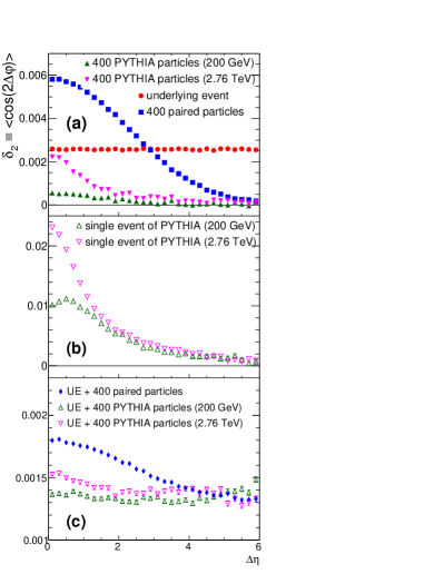
Figure 15: (Color online) $\delta_{2}$ as a function of $\Delta\eta$ for different classes of particles in the simple Monte-Carlo simulations. Panel (a) includes the underlying event without nonflow, the simple nonflow implementation with 400 paired particles, and two cases of 400 PYTHIA particles from p+p collisions at $\sqrt{s}=200$ GeV and 2.76 TeV, respectively. The results from single PYTHIA events are presented in panel (b).

The nonflow effects can be easily visualized in the correlation function between two particles, $\delta_{2}\equiv\langle\cos[2(\varphi_{1}-\varphi_{2})]\rangle$, as a function of their $\eta$ gap ($\Delta\eta$). Without nonflow or decorrelation, $\delta_{2}$ simply reflects $\langle v_{2}^{2}\rangle$. Figure 15(a) presents $\delta_{2}(\Delta\eta)$ for four distinct classes of particles without decorrelation in the simple Monte Carlo simulation. The 1000 particles in each underlying event uniformly cover the $\eta$ range of $(-5,5)$, and carry an average $v_{2}$ of 5%. From event to event, $v_{2}$ follows a uniform distribution from 3.5% to 6.5%. Since the underlying events are free of nonflow, the corresponding $\delta_{2}$ remains constant at $\langle v_{2}\rangle^{2}+\sigma^{2}$, where $\sigma\sim 0.75\%$ is due to the event-by-event fluctuation. The second class consists of 400 paired particles without elliptic flow. Within each of the 200 pairs, the two particles have the same azimuthal angle, and their $\Delta\eta$ follows a Gaussian distribution with zero mean and a width of 2 units of $\eta$. Although the mean values of $\delta_{2}$ are almost identical for the 1000 underlying-event particles and the 400 paired particles, the $\Delta\eta$ dependence is very different between these two cases. The former is constant, whereas the latter is enhanced at small $\Delta\eta$, and approaches zero at large $\eta$ gaps. The result from the simple nonflow implementation qualitatively resembles the correlation between the 400 PYTHIA particles (triangular markers), with stronger effects. On average, the combination of 21(12) single PYTHIA events of p+p collisions at 200 GeV(2.76 TeV) provides the 400 PYTHIA particles. Although a single PYTHIA event has very strong nonflow effects as shown in panel (b), the correlation strength is diluted roughly by a factor of 21 or 12, when such a number of PYTHIA events are merged together. Interestingly, the single PYTHIA events of different collision energies illustrate similar long-range correlations at $\Delta\eta>1$. Finally, panel (c) shows the correlation results after the “nonflow” particles are embedded into the underlying events. In general, the embedded events display lower $\delta_{2}$ values than the underlying events, since the 400 particles with no flow dilute the 1000 flowing particles. Meanwhile, nonflow correlations cause the nonuniform $\Delta\eta$ dependence. In practice, the simple Monte Carlo simulation can be tuned to compare with real data, and help us understand the nonflow contributions.

Appendix B Cumulant of four-angle correlations

The two-variable cumulant of an observable, $f=xy$, is defined as

$$\langle\langle xy\rangle\rangle\equiv\langle xy\rangle-\langle x\rangle\langle y\rangle.$$ (19)

The first term computes the average of the product, accounting for correlations between $x$ and $y$, while the second gives the product of the averages, keeping $x$ and $y$ independent of each other. A zero cumulant means that $x$ and $y$ are independent with no correlation. The $T_{2}$ observable involves four azimuthal angles, and therefore we derive the four-variable cumulant, which subtracts all lower-order correlations:

$$\langle\langle xyzt\rangle\rangle \equiv \langle xyzt\rangle-\langle\langle xyz\rangle\rangle\langle t\rangle-\langle\langle xyt\rangle\rangle\langle z\rangle$$ (20)

$$-\langle\langle xzt\rangle\rangle\langle y\rangle-\langle\langle yzt\rangle\rangle\langle x\rangle-\langle\langle xy\rangle\rangle\langle\langle zt\rangle\rangle$$

$$-\langle\langle xz\rangle\rangle\langle\langle yt\rangle\rangle-\langle\langle xt\rangle\rangle\langle\langle yz\rangle\rangle$$

$$-\langle x\rangle\langle y\rangle\langle z\rangle\langle t\rangle.$$

In principle, we should obtain the three-variable cumulants before calculating the four-variable cumulant. However, in the case of $T_{2}$, all the variables can be expressed as a sine or cosine function of an azimuthal angle, and we can force $\langle x\rangle=\langle y\rangle=\langle z\rangle=\langle t\rangle=0$ in the data analyses, e.g., via the shifting method [22]. Thus, Eq. 20 is simplified to

$$\langle\langle xyzt\rangle\rangle=\langle xyzt\rangle-\langle xy\rangle\langle zt\rangle-\langle xz\rangle\langle yt\rangle-\langle xt\rangle\langle yz\rangle.$$ (21)

The numerator of $T_{2}$ can be expanded into four terms:

$$\sin(a-b)\sin(c-d)$$ (22)

$$= \sin(a)\cos(b)\sin(c)\cos(d)$$

$$-\sin(a)\cos(b)\sin(d)\cos(c)$$

$$-\sin(b)\cos(a)\sin(c)\cos(d)$$

$$+\sin(b)\cos(a)\sin(d)\cos(c).$$

We put the first term into Eq. 21 as an example,

$$\langle\langle\sin(a)\cos(b)\sin(c)\cos(d)\rangle\rangle$$ (23)

$$= \langle\sin(a)\cos(b)\sin(c)\cos(d)\rangle$$

$$-\langle\sin(a)\sin(c)\rangle\langle\cos(b)\cos(d)\rangle,$$

where terms such as $\langle\sin(a)\cos(b)\rangle$ vanish in symmetric heavy-ion collisions. Using the product-to-sum formulas, we have

$$\langle\sin(a)\sin(c)\rangle\langle\cos(b)\cos(d)\rangle$$ (24)

$$= \frac{1}{4}[\langle\cos(a-c)\rangle\langle\cos(b-d)\rangle$$

$$+\langle\cos(a-c)\rangle\langle\cos(b+d)\rangle$$

$$-\langle\cos(a+c)\rangle\langle\cos(b-d)\rangle$$

$$\langle\cos(a+c)\rangle\langle\cos(b+d)\rangle].$$

Only the cosines with arguments of the angle difference are independent of the coordinate system, and may render finite averages. Hence Eq. 23 becomes

$$\langle\langle\sin(a)\cos(b)\sin(c)\cos(d)\rangle\rangle$$ (25)

$$= \langle\sin(a)\cos(b)\sin(c)\cos(d)\rangle$$

$$-\frac{1}{4}\langle\cos(a-c)\rangle\langle\cos(b-d)\rangle.$$

We follow the same procedure for the other three terms in Eq. 22 and obtain

$$\langle\langle\sin(a-b)\sin(c-d)\rangle\rangle$$ (26)

$$\equiv \langle\sin(a-b)\sin(c-d)\rangle-\frac{1}{2}\langle\cos(a-c)\rangle\langle\cos(b-d)\rangle$$

$$+\frac{1}{2}\langle\cos(a-d)\rangle\langle\cos(b-c)\rangle.$$

Appendix C Generalization of $T_{2}$

In the $T_{2}$ analyses in Sec. IV, we randomly split particles within $|\eta|<1$ into two sub-events, and reconstruct $\Psi_{\rm m,1}$ and $\Psi_{\rm m,2}$ based on them. By this means, $\Psi_{\rm m,1}$ and $\Psi_{\rm m,2}$ are indistinguishable, sharing the same kinematic region, bearing the same event plane resolution, and tilting in the same way. In general, $\Psi_{\rm m,1}$ and $\Psi_{\rm m,2}$ could come from different $\eta$ ranges, e.g., with $-1<\eta_{\rm m,1}<0$ and $0<\eta_{\rm m,2}<1$. Accordingly, the definition of $T_{2}$ is not unique any more, with a few possible combinations. For example, we can define

$$T_{2(I)}=\frac{\langle\langle\sin 2(\Psi_{\rm f}-\Psi_{{\rm m},2})\sin 2(\Psi_{\rm b}-\Psi_{{\rm m},1})\rangle\rangle}{\langle\cos 2(\Psi_{\rm f}-\Psi_{{\rm m},2})\rangle\langle\cos 2(\Psi_{\rm b}-\Psi_{{\rm m},1})\rangle},$$ (27)

and within the frame work of the simple Monte Carlo simulation, where the tilt angle linearly increases with the $\eta$ gap, we have

$$T_{2(I)} = -\frac{1}{2}\tan^{2}[2\frac{d\Delta\Psi}{d\eta}(|\eta_{\rm f(b)}|-0.5)]{\rm~{}(S~{}shape)},$$ (28)

$$T_{2(I)} = \frac{1}{2}\tan^{2}[2\frac{d\Delta\Psi}{d\eta}(|\eta_{\rm f(b)}|-0.5)]{\rm~{}(C~{}shape)}.$$ (29)

We can switch $\Psi_{\rm m,1}$ and $\Psi_{\rm m,2}$ in $T_{2(I)}$ to define a new observable

$$T_{2(II)}=\frac{\langle\langle\sin 2(\Psi_{\rm f}-\Psi_{{\rm m},1})\sin 2(\Psi_{\rm b}-\Psi_{{\rm m},2})\rangle\rangle}{\langle\cos 2(\Psi_{\rm f}-\Psi_{{\rm m},1})\rangle\langle\cos 2(\Psi_{\rm b}-\Psi_{{\rm m},2})\rangle},$$ (30)

and with the constant $\frac{d\Delta\Psi}{d\eta}$, we have

$$T_{2(II)} = -\frac{1}{2}\tan^{2}[2\frac{d\Delta\Psi}{d\eta}(|\eta_{\rm f(b)}|+0.5)]{\rm~{}(S~{}shape)},$$ (31)

$$T_{2(II)} = \frac{1}{2}\tan^{2}[2\frac{d\Delta\Psi}{d\eta}(|\eta_{\rm f(b)}|-0.5)]{\rm~{}(C~{}shape)}.$$ (32)

A third type of $T_{2}$ observable can be defined as

$$T_{2(III)}=\frac{\langle\langle\sin 2(\Psi_{\rm f}-\Psi_{\rm b})\sin 2(\Psi_{\rm m,1}-\Psi_{{\rm m},2})\rangle\rangle}{\langle\cos 2(\Psi_{\rm f}-\Psi_{\rm b})\rangle\langle\cos 2(\Psi_{\rm m,1}-\Psi_{{\rm m},2})\rangle},$$ (33)

which is zero for the C-shaped decorrelation. With the constant $\frac{d\Delta\Psi}{d\eta}$, the expectation from the S-shaped case is

$$T_{2(III)}=-\frac{1}{2}\tan(2\frac{d\Delta\Psi}{d\eta})\tan(4\frac{d\Delta\Psi}{d\eta}|\eta_{\rm f(b)}|).$$ (34)

References

- [1] S. Voloshin and Y. Zhang, Z. Phys. C 70, 665 (1996).
- [2] A. M. Poskanzer and S. A. Voloshin, Phys. Rev. C 58, 1671 (1998).
- [3] U. Heinz and R. Snellings, Ann. Rev. Nucl. Part. Sci. 63, 123 (2013).
- [4] P. Bozek, W. Broniowski, and J. Moreira, Phys. Rev. C 83, 034911 (2011).
- [5] A. Behera, M. Nie, and J. Jia, (2020), Phys. Rev. Res. 2, 023362 (2020).
- [6] L.-G. Pang, G.-Y. Qin, V. Roy, X.-N. Wang, and G.-L. Ma, Phys. Rev. C 91, 044904 (2015).
- [7] B. Schenke and S. Schlichting, Phys. Rev. C 94, 044907 (2016).
- [8] Shen, Chun and Schenke, Bjorn, Phys. Rev. C 97, 024907 (2018).
- [9] V. Khachatryan et al. [CMS Collaboration], Phys. Rev. C 92, 034911 (2015).
- [10] M. Aaboud et al. [ATLAS Collaboration], Eur. Phys. J. C 78, 142 (2018).
- [11] G. Aad et al. [ATLAS Collaboration], Phys. Rev. Lett. 126, 122301 (2021).
- [12] M. Nie [STAR Collaboration], Nucl. Phys. A 1005, 121783 (2021).
- [13] P. Bozek and W. Broniowski, Phys. Rev. C 97, 034913 (2018).
- [14] A. Sakai, K. Murase, T. Hirano, Phys. Rev. C 102, 064903 (2020).
- [15] Z.-W. Lin, C.M. Ko, B.-A. Li, B. Zhang, S. Pal, Phys. Rev. C 72, 064901 (2005).
- [16] C. Adler et al. [STAR Collaboration], Phys. Rev. C 66, 034904 (2002).
- [17] T. Sjostrand, S. Mrenna, and P. Z. Skands, JHEP 05, 026 (2006).
- [18] X.-N. Wang and M. Gyulassy, Phys. Rev. D 44, 3501 (1991).
- [19] B. Zhang, Comput. Phys. Commun. 109, 193 (1998).
- [20] B. A. Li and C. M. Ko, Phys. Rev. C 52, 2037 (1995).
- [21] Zi-Wei Lin, Phys. Rev. C 90, 014904 (2014).
- [22] J. Barrette et al. [E877 Collaboration], Phys. Rev. C 56, 3254 (1997).