Clustered Sparse Channel Estimation for Massive MIMO Systems by Expectation Maximization-Propagation (EM-EP)

Abstract

We study the problem of downlink channel estimation in multi-user massive multiple input multiple output (MIMO) systems. To this end, we consider a Bayesian compressive sensing approach in which the clustered sparse structure of the channel in the angular domain is employed to reduce the pilot overhead. To capture the clustered structure, we employ a conditionally independent identically distributed Bernoulli-Gaussian prior on the sparse vector representing the channel, and a Markov prior on its support vector. An expectation propagation (EP) algorithm is developed to approximate the intractable joint distribution on the sparse vector and its support with a distribution from an exponential family. The approximated distribution is then used for direct estimation of the channel. The EP algorithm assumes that the model parameters are known a priori. Since these parameters are unknown, we estimate these parameters using the expectation maximization (EM) algorithm. The combination of EM and EP referred to as EM-EP algorithm is reminiscent of the variational EM approach. Simulation results show that the proposed EM-EP algorithm outperforms several recently-proposed algorithms in the literature.

I Introduction

In FDD-based massive MIMO systems, downlink (DL) channel estimation is quite challenging [1]. In the conventional pilot-based method, the length of the pilot sequence scales with the number of transmitting antennas. This implies a long pilot sequence which results in reduced spectral efficiency. Moreover, the time required for pilot and data transmission may exceed the coherence time of the channel. Recently, compressive sensing (CS) [2, 3] has been explored to reduce the pilot-overhead. Due to the limited local scattering in the propagation environment, massive MIMO channel has a sparse representation in the discrete Fourier transform (DFT) basis [4, 1, 5, 6]. Using this sparsity structure, many CS-based estimation algorithms have been devised. The classical orthogonal matching pursuit (OMP) [7] and compressive sampling matching pursuit (CoSaMP) [8] are investigated in [9, 10]. In [11] the authors assumed a common spatial sparsity among the subcarriers in a frequency-selective DL channel and proposed the distributed sparsity adaptive matching pursuit (DSAMP). Using a similar common spatial sparsity assumption, a generalized approximate message passing (GAMP) based algorithm is proposed in [12] and the sparse Bayesian learning (SBL) algorithm is derived in [13, 14]. These and other algorithms which use a DFT basis to obtain the sparse representation, employ a fixed uniformly-spaced discrete grid in the angular domain which may not be sufficiently dense. As a result, some of the physical angles of departures (AoDs) of the massive MIMO channel may not lie on the assumed grid points. This direction mismatch error, also known as channel modeling error, causes leakage of energy from such physical AoDs into the nearby angular bins resulting in a straddle performance loss. In [15, 16] this modeling error is minimized by learning a better over-complete dictionary for the sparse representation. However, the proposed algorithm requires extensive channel measurements from several locations in the cell to be used as training samples. These measurements are cell-specific and difficult to collect in practice. In [17], an Off-grid SBL algorithm is proposed in which the sampled grid points are modeled as continuous-valued parameters and are learned iteratively to reduce the modeling error. Simulation results in [17] show improved performance of off-grid SBL compared to the over-complete dictionary learning algorithm in [15].

SBL and off-grid SBL aim to recover the sparse vector coefficients individually by modeling them with an independent and identically distributed (iid) Gaussian prior distribution. However, according to the geometry-based stochastic channel model (GSCM) [18], there are a few dominant scatterers in the propagation environment, and the sub-paths from each scatterer concentrate in small angular spreads which appear as non-zero clusters in the sparse representation. This model is used in [19], although with the stringent assumption of uniformly-sized clusters in the sparse vector. For non-uniform burst sparsity, a pattern-coupled SBL (PC-SBL) algorithm is proposed in [21] in which the precision of each coefficient in the sparse vector is tuned according to the precision of its immediate neighbors. However, PC-SBL updates the precisions with a sub-optimal solution. To avoid this sub-optimality, a generic version of PC-SBL is derived in [20], referred to as PC-VB here, where the authors assigned a latent support vector to every coefficient in the sparse vector and assumed a multinoulli prior on the support vector. The resulting joint posterior distribution on the sparse vector and its support is approximated with a variational Bayes-based algorithm [22]. Grid refining procedure from [17] is also used to mitigate the direction mismatch errors. In the same vein, Turbo compressive sensing (TCS) algorithm and expectation maximization based GAMP algorithm were proposed in [23] and [24], respectively, in which the sparse vector coefficients are modeled with an iid Bernoulli-Gaussian (BG) prior. In [10] the authors extended [23] for the clustered sparse structure of the massive MIMO channel and proposed a structured turbo compressive sensing (S-TCS) algorithm. With a conditional iid BG prior on the sparse vector, a Markov prior is assumed on its support to integrate the clustering information of the massive MIMO channel. In [25], a super-resolution clustered sparse Bayesian learning (SuRe-CSBL) algorithm is proposed for a Markov prior distribution on the support vector. SuRe-CSBL approximates the true joint posterior distribution on the sparse vector and its support with a structured GAMP algorithm. The approximated distribution is then used for the estimation of massive MIMO channel. The grid refining method from [17] is also integrated into SuRe-CSBL.

In this paper, we propose an expectation propagation (EP) algorithm to estimate the clustered sparse vector representing the massive MIMO channel. Once the sparse vector is estimated from the received signal, the physical massive MIMO channel can be easily estimated by a transform operation on the sparse vector as in [20, 10, 25]. The contributions made in this paper are summarized as follow:

• Expectation propagation (EP) algorithm [26, 27] has been recently applied to SIMO and MIMO channel estimation [28, 29, 30, 31]. It has also been applied to solve the inference problem in the CS literature [32]. In [33], the authors used an EP algorithm to approximate the true joint posterior distribution on the sparse vector and its support with a distribution from an exponential family. However, an iid Bernoulli prior is assumed on the support vector which does not capture the clustered structure of the sparse vector. In [34] the authors assumed that the partitioning of the cluster in the sparse vector is known a priori and modeled each cluster with a different Bernoulli prior distribution. In contrast, we assume here that the cluster partitioning in the sparse vector is unknown. Therefore to capture the structure of the sparse vector we model its support vector with a first-order Markov process. An EP algorithm is developed to iteratively approximate the intractable true joint posterior distribution on the sparse vector and its support with a distribution from an exponential family. This distribution is then used for the direct estimation of the DL massive MIMO channel.

• The framework of EP algorithm in [34, 33] assumes that the model parameters including the noise precision in the signal model, the hyperparameters in the prior distribution on the sparse vector, and the hyperparameters in the prior distribution on the support vector are known a priori. For practical massive MIMO channel, these parameters are unknown and need to be estimated. One way to estimate the model parameters is by maximizing the marginal likelihood function$-$the procedure which is known as type-II maximum likelihood method or evidence procedure [14]. However, directly maximizing the marginal likelihood function does not result in closed-form update equations for the model parameters [13, 14]. Thus we derive an expectation maximization (EM) algorithm which results in closed-form update equations and iteratively computes the maximum likelihood solution of the model parameters [35, 36].

• In order to integrate the EP algorithm with the EM algorithm, we use a variational EM approach [37, 38] in which the approximated joint posterior distribution by the EP algorithm is used to compute the expectation step in the EM algorithm. The convergence of the resulting EM-EP algorithm is guaranteed through the convergence properties of the variational EM algorithm [37]. As iterations of the proposed method proceed, the EM algorithm converges to a local maxima of the marginal likelihood function [35] and the EP algorithm closely approximates the true joint posterior distribution with a distribution from an exponential family [39]. Grid refining procedure from [20, 17] is also integrated in the proposed EM-EP algorithm to reduce the channel modeling error.

• Extensive simulations are carried out to demonstrate the efficacy of the proposed EM-EP algorithm. The results are also compared with those in the literature showing the advantages of the proposed method.

This paper is organized as follow. Section II describes the system model for the FDD-based downlink channel estimation in multi-user massive MIMO system. Expectation propagation algorithm for this system is proposed in Section III. An expectation maximization algorithm to estimate the model parameters and to refine the grid is derived in Section IV. Simulation results are discussed in Section V, and Section VI concludes the paper.

Notations: Throughout this paper, small letters $(x)$ are used for scalars, bold small letters $(\mathbf{x})$ for vectors, and bold capital letters $(\mathbf{X})$ for matrices. $\mathbb{R}$ and $\mathbb{C}$ represent the set of real and complex numbers, respectively. The superscripts $(.)^{T}$, $(.)^{H}$, $(.)^{*}$, and $(.)^{-1}$ represent transpose, Hermitian transpose, complex conjugate, and inverse operations, respectively. $\mathcal{CN}(\mathbf{x};\bm{\mu},\bm{\Sigma})$ denotes complex Gaussian distribution on $\mathbf{x}$ with mean $\bm{\mu}$ and covariance matrix $\bm{\Sigma}$. $\text{Bern}(x;p)$ denotes a Bernoulli distribution on $x$ with mean $p$. For a complex variable $x$, $\lvert x\rvert$, $\Re\{x\}$ and $\Im\{x\}$ represent its modulus, real part and imaginary part, respectively. For a probability density function (pdf) $p(.)$, $\mathbb{E}_{p}$ denotes the expectation operator with respect to $p(.)$. $\delta(x)$ is the Kronecker delta function which is equal to $1$ when $x=0$ and is zero otherwise. $\mathbf{I}_{N}$ denotes the $N\times N$ identity matrix. Finally, tr$(\mathbf{X})$ and $||\mathbf{x}||$ denote the trace of a matrix $\mathbf{X}$ and the $\ell_{2}$-norm of the vector $\mathbf{x}$, respectively.

II System Model

Consider a single cell massive MIMO system where a BS equipped with $G$ antennas serves $K$ users each one having a single antenna. It is assumed that FDD is used and to enable the estimation of the DL channels, the BS broadcasts a sequence of $N$ pilot symbols denoted by $\mathbf{X}=[\mathbf{x}_{1},\mathbf{x}_{2},\ldots,\mathbf{x}_{N}]^{H}$ where $\mathbf{x}_{n}\in\mathbb{C}^{G\times 1}$ for $n=1,\ldots,N$. The signal received by the $k$-th user is given by

$$\mathbf{y}_{k}=\mathbf{X}\mathbf{h}_{k}+\mathbf{n}_{k},$$ (1)

where $\mathbf{y}_{k}\in\mathbb{C}^{N\times 1}$, $\mathbf{h}_{k}\in\mathbb{C}^{G\times 1}$ is the DL channel to the $k$-th user and the receiver noise $\mathbf{n}_{k}$ is distributed as $\mathcal{CN}(\mathbf{n}_{k};\mathbf{0},\eta^{-1}_{k}\mathbf{I}_{N})$ in which $\eta_{k}$ denotes the precision.

Assuming that the transmitted pilot sequence satisfies $\mathrm{tr}(\mathbf{X}\mathbf{X}^{H})=NG$, the signal-to-noise ratio (SNR) is given by $SNR=\eta_{k}$. Suppose that the BS is equipped with a uniform linear array (ULA) and to transmit in the direction $\theta$, it uses the beam steering vector

$$\mathbf{a}(\theta)=\left[1,e^{-j2\pi\frac{d}{\lambda_{d}}\text{sin}(\theta)},\ldots,e^{-j2\pi\frac{d}{\lambda_{d}}(G-1)\text{sin}(\theta)}\right]^{T},$$ (2)

where $d$ is the spacing between adjacent antenna elements and $\lambda_{d}$ is the wavelength of the DL signal. Let the DL signal propagating from BS on the way to the $k$-th user pass across a total of $L_{s}$ scatterers each one forwarding the signal on $L_{p}$ paths towards the user. Then the channel vector $\mathbf{h}_{k}$ to the $k$-th user can be written as

$$\mathbf{h}_{k}=\sum^{L_{s}}_{s=1}\sum^{L_{p}}_{p=1}\alpha_{k,s,p}\mathbf{a}(\theta_{k,s,p}),$$ (3)

where $\alpha_{k,s,p}$ is the complex path gain for the $s$-th scatterer and $p$-th path, and $\theta_{k,s,p}$ is the corresponding AoD [40, 5].

To reduce the pilot-overhead for estimating this downlink channel, we use the CS approach which requires a virtual channel representation of the physical channel in (3). To this end, let $\bm{\theta}=\left(\theta_{1},\theta_{2},\ldots,\theta_{M}\right)^{T}$ denote a uniform sampling of the interval $[-\pi/2,\pi/2]$ into $M$ points. Assuming $M$ is large enough such that the physical AoDs in (3) lie on the grid points, the virtual representation of $\mathbf{h}_{k}$ is given by

$$\mathbf{h}_{k}=\mathbf{A}(\bm{\theta})\mathbf{w}_{k},$$ (4)

where $\mathbf{A}(\bm{\theta})=\left[\mathbf{a}\left({\theta}_{1}\right),\mathbf{a}\left({\theta}_{2}\right),\ldots,\mathbf{a}\left({\theta}_{M}\right)\right]$ and the vector $\mathbf{w}_{k}$ contains the channel coefficients in the virtual angular domain. Note that when $M=G$ and the grid is uniformly sampled, the dictionary $\mathbf{A}(\bm{\theta})$ represents the unitary discrete Fourier transform matrix [17]. The choice of the parameter $M$ is discussed in Section V.

In this paper, we focus on the DL channel estimation for a reference user. Therefore dropping the index $k$, from (1) and (4), the received signal is written as

$$\mathbf{y}=\bm{\Phi}(\bm{\theta})\mathbf{w}+\mathbf{n},$$ (5)

in which $\bm{\Phi}(\bm{\theta})=\mathbf{X}\mathbf{A}(\bm{\theta})$. From (5) the likelihood function of $\mathbf{w}$ is given as $p(\mathbf{y}|\bm{\Phi}(\bm{\theta}),\mathbf{w},\eta)$$=\mathcal{CN}(\mathbf{y};\bm{\Phi}(\bm{\theta})\mathbf{w},\eta^{-1}\mathbf{I}_{N})$. Given $\mathbf{y}$ and $\bm{\Phi}(\bm{\theta})$ we aim to compute the posterior distribution of the sparse vector $\mathbf{w}$. Note that the posterior distribution on $\mathbf{w}$ can be used to find the minimum mean squared error (MMSE) estimate of $\mathbf{w}$ from which the physical channel estimate is obtained using (4).

According to the GSCM model [18], there are only a few dominant scatterers in the channel, i.e., $L_{s}$ is small. Moreover, the forwarding paths from each scatterer are concentrated in a small angular spread around the line of sight direction between the BS and the scatterer [15, 41]. Thus, $\mathbf{w}$ exhibits a clustered sparse structure with unknown marking of cluster boundaries. Hence the support (indices of non-zero elements) of $\mathbf{w}$ is unknown [17, 25, 20]. To model the clustered sparse structure of $\mathbf{w}$ and to determine its support, we condition the $m$-th element of $\mathbf{w}$ on a latent variable $z_{m}\in\{0,1\}$, where $w_{m}\neq 0$ when $z_{m}=1$ and $w_{m}=0$ when $z_{m}=0$. Thus given the latent vector $\mathbf{z}=[z_{1},z_{2},\ldots,z_{M}]^{T}$, as in [10, 25, 34, 33], the prior distribution on $\mathbf{w}$ is written as

$$p(\mathbf{w}|\mathbf{z},\bm{\gamma})=\prod^{M}_{m=1}p(w_{m}|z_{m},\gamma_{m})=\prod^{M}_{m=1}\left[z_{m}\mathcal{CN}(w_{m};0,\gamma^{-1}_{m})+(1-z_{m})\delta(w_{m})\right],$$ (6)

where $\bm{\gamma}=(\gamma_{1},\gamma_{2},\ldots,\gamma_{M})^{T}$ and $\gamma_{m}$ is the precision of $w_{m}$. Due to the clustered sparsity of $\mathbf{w}$, the elements of the vector $\mathbf{z}$ are correlated. To capture this correlation we model $\mathbf{z}$ as a first-order Markov process with transition probabilities $Pr(z_{m}=1|z_{m-1}=0)=\tau_{01}$ and $Pr(z_{m}=0|z_{m-1}=1)=\tau_{10}$. Note that these transition probabilities reflect the clustered sparse structure of $\mathbf{w}$ in the following way. The average length of the sequence of zeros between two consecutive non-zero clusters is large when $\tau_{01}$ is small, and the non-zero cluster size on average is large when $\tau_{10}$ is small. Denoting $\bm{\tau}\triangleq(\tau_{01},\tau_{10})$, the prior distribution on $\mathbf{z}$ is given as

$$p(\mathbf{z}|\bm{\tau})=p(z_{1})\prod^{M}_{m=2}p(z_{m}|z_{m-1},\bm{\tau})$$

$$=p(z_{1})\prod^{M}_{m=2}\left[\left((1-\tau_{10})^{z_{m-1}}(\tau_{01})^{(1-z_{m-1})}\right)^{z_{m}}\right.\left.\left((\tau_{10})^{z_{m-1}}(1-\tau_{01})^{(1-z_{m-1})}\right)^{(1-z_{m})}\right],$$ (7)

where $p(z_{1})=\text{Bern}(z_{1};\lambda)$ and we use the steady state distribution for $z_{1}$ and set $\lambda=\frac{\tau_{01}}{\tau_{01}+\tau_{10}}$.

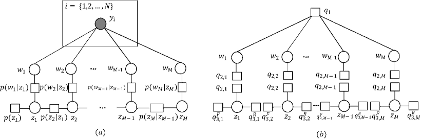
Figure 1: Factor graph illustrations of $(a)$ True posterior distribution in (9), and $(b)$ Approximated posterior distribution in (20). Variable nodes are represented by circles (filled in circles for observed variables and empty ones for the hidden variables) and factor nodes are denoted by small rectangles. Repetition of observed variables in the subgraph is represented using a plate (big rectangle) notation.

In practice the physical AoDs may not lie on the assumed angular grid $\bm{\theta}$ in (4), and thus we treat $\bm{\theta}$ as an unknown parameter and aim to estimate it for learning the dictionary. Therefore, letting $\bm{\xi}\triangleq(\bm{\tau},\gamma_{1},\gamma_{2},\ldots,\gamma_{M},\eta,\bm{\theta}^{T})^{T}$, we aim to jointly estimate $(\mathbf{w},\mathbf{z},\bm{\xi})$. We write the joint posterior distribution of $(\mathbf{w},\mathbf{z},\bm{\xi})$ as

$$p(\mathbf{w},\mathbf{z},\bm{\xi}|\mathbf{y}) \propto p(\mathbf{w},\mathbf{z}|\mathbf{y},\bm{\xi})p(\mathbf{y}|\bm{\xi})p(\bm{\xi}),$$ (8)

where the conditioning on $\bm{\xi}$ in (8) removes the multidimensional integration over $\bm{\xi}$ required otherwise in computing the normalization constant. Note that in (8), the marginal joint posterior distribution on $\mathbf{w}$ and $\mathbf{z}$ is given by

$$p(\mathbf{w},\mathbf{z}|\mathbf{y},{\bm{\xi}})\propto p(\mathbf{y}|\bm{\Phi}(\bm{\theta}),\mathbf{w},{\eta})p(\mathbf{w}|\mathbf{z},{\bm{\gamma}})p(\mathbf{z}|\bm{\tau}),$$ (9)

Computing the joint posterior distribution in (8) is still involved. We can reduce (8) to (9) by using the maximum a posteriori estimate of ${\bm{\xi}}$ in (9) obtained by maximizing $p(\mathbf{y}|\bm{\xi})p(\bm{\xi})$ with respect to $\bm{\xi}$. Assuming a uniform prior distribution on $\bm{\xi}$, we get the maximum likelihood (ML) estimate which can be computed as follows.

$$\quad\hat{\bm{\xi}} =\operatorname*{arg\,max}_{\bm{\xi}}p(\mathbf{y}|\bm{\xi}),$$ (10)

The objective function in (10) is a non-concave function and due to the involved multidimensional parameter space a brute-force search is difficult [14]. An alternative is to use the iterative expectation maximization (EM) algorithm which increases the likelihood function $p(\mathbf{y}|\bm{\xi})$ in each iteration and guarantees convergence to a local maxima [36, 35]. To this end we define the complete data as $\mathbf{d}=[\mathbf{y}^{T},\mathbf{w}^{T},\mathbf{z}^{T}]^{T}$. Then if $\bm{\xi}^{l}$ is the estimate from the $l$-th iteration, in the $(l+1)$-st iteration of EM we perform the following two steps

$$\text{E-Step}:\ {\mathcal{L}}(\bm{\xi};\bm{\xi}^{l})=\mathbb{E}_{p(\mathbf{w},\mathbf{z}|\mathbf{y},\bm{\xi}^{l})}\left[\ln p(\mathbf{y},\mathbf{w},\mathbf{z}|\bm{\xi})\right],$$ (11)

$$\text{M-Step}:\ \bm{\xi}^{(l+1)}=\operatorname*{arg\,max}_{\bm{\xi}}{\mathcal{L}}(\bm{\xi};\bm{\xi}^{l}),$$ (12)

and (11) and (12) are repeated until convergence.

Computing the E-step in (11) requires the exact joint posterior distribution $p(\mathbf{w},\mathbf{z}|\mathbf{y},\bm{\xi}^{l})$ which is computationally intractable as it requires a multidimensional integration and summation. Therefore in Section III we derive an expectation propagation (EP) algorithm to approximate this distribution with a distribution from an exponential family. We denote the approximate distribution by $Q(\mathbf{w},\mathbf{z}|\mathbf{y},\bm{\xi}^{l})$ and use it in place of $p(\mathbf{w},\mathbf{z}|\mathbf{y},\bm{\xi}^{l})$ in (11). Note that the estimate of the parameters in the $l$-th iteration of EM, namely $\bm{\xi}^{l}$ is used by the EP algorithm to obtain $Q(\mathbf{w},\mathbf{z}|\mathbf{y},\bm{\xi}^{l})$. Once the E-step is solved in this way, the solution to the M-step, derived in Section IV, is computed to obtain $\bm{\xi}^{l+1}$. Next the EP algorithm is run with $\bm{\xi}^{l+1}$ to obtain $Q(\mathbf{w},\mathbf{z}|\mathbf{y},\bm{\xi}^{l+1})$ which is used in the $(l+1)$-st iteration of E-step. The iterations between EM and EP are continued in this way until convergence is achieved. This EM-EP approach is reminiscent of the variational EM algorithm [37, 38]. We should point out that convergence of EM-EP is assured based on the convergence properties of variational EM [37]. In particular, as the iterations of the EM-EP proceed, the EM algorithm converges to a local maxima of the objective function in (10) [35] and the EP algorithm closely approximates the true joint posterior distribution $p(\mathbf{w},\mathbf{z}|\mathbf{y},\bm{\xi}^{l})$ in (9) [39]. An EM-EP algorithm has been used in [42] to solve a classification problem, whereas here we tend to use the setting for solving the estimation problem.

III Expectation Propagation algorithm

In this section, we derive an expectation propagation algorithm to approximate the joint posterior distribution $p(\mathbf{w},\mathbf{z}|\mathbf{y},\bm{\xi})$ in (9) with a distribution from an exponential family. For a review of the EP algorithm we refer the reader to [26, 27, 32, 34, 33].

Let $\mathcal{F}$ denote the family of exponential distributions. Exploiting the factorized structure of (9), we approximate the joint posterior distribution $p(\mathbf{w},\mathbf{z}|\mathbf{y},\bm{\xi})$ with

$$Q(\mathbf{w},\mathbf{z})=Q(\mathbf{w})Q(\mathbf{z}),$$ (13)

where $Q(\mathbf{w})\in\mathcal{F}$ and $Q(\mathbf{z})\in\mathcal{F}$. We choose the factors in (13) as

$$Q(\mathbf{w}) =\mathcal{CN}(\mathbf{w};\bm{\mu},\bm{\Sigma}),$$ (14)

$$Q(\mathbf{z}) =\prod^{M}_{m=1}Q_{m}(z_{m})=\prod^{M}_{m=1}\text{Bern}(z_{m};\sigma(p_{m})),$$ (15)

where the sigmoid function $\sigma(.)$ is used to define the mean of the Bernoulli distribution as $\sigma(p_{m})$. The use of sigmoid function simplifies EP updates and avoids numerical underflow errors resulting in the numerical stability of EP algorithm [34]. In (14) and (15), $\bm{\mu}$, $\bm{\Sigma}$, and $\mathbf{p}\triangleq[p_{1},p_{2},\ldots,p_{M}]^{T}$ are the unknown parameters that we next aim to estimate with the EP algorithm.

Next we approximate each factor in (9). Let $q_{1}(\mathbf{w})$, $q_{2}(\mathbf{w},\mathbf{z})$ and $q_{3}(\mathbf{z})$ approximate
$p(\mathbf{y}|\bm{\Phi}(\bm{\theta}),\mathbf{w},\eta)$, $p(\mathbf{w}|\mathbf{z},\bm{\gamma})$ and $p(\mathbf{z}|\bm{\tau})$, respectively. Since $q_{1}(.)$ and $q_{3}(.)$ are the marginal functions of $\mathbf{w}$ and $\mathbf{z}$, respectively, whereas $q_{2}(.)$ is the joint function of both $\mathbf{w}$ and $\mathbf{z}$, we choose these terms as follows

$$q_{1}(\mathbf{w}) =\mathcal{CN}(\mathbf{w};\bm{\mu}_{1},\bm{\Sigma}_{1}),$$ (16)

$$q_{2}(\mathbf{w},\mathbf{z}) =\prod^{M}_{m=1}q_{2,m}(w_{m},z_{m}),$$ (17)

where

$$q_{2,m}(w_{m},z_{m})\propto\mathcal{CN}(w_{m};\mu_{2,m},\Sigma_{2,m})\text{Bern}(z_{m};\sigma(p_{2,m})),$$ (18)

For $q_{3}(\mathbf{z})$, we approximate $p(z_{m}|z_{m-1})$ in (II) with $q^{FR}_{3,m-1,m}(z_{m-1},z_{m})$ which in factorized form we write as $q^{FR}_{3,m-1,m}(z_{m-1},z_{m})=q^{R}_{3,m-1}(z_{m-1})q^{F}_{3,m}(z_{m})$. Therefore

$$q_{3}(\mathbf{z}) =\prod^{M}_{m=1}q^{R}_{3,m}(z_{m})q^{F}_{3,m}(z_{m}),$$ (19)

where for $j\in\{F,R\}$, $q^{j}_{3,m}(z_{m})$$=\text{Bern}\big{(}z_{m};\sigma(p^{j}_{3,m})\big{)}$ and $\sigma(p^{j}_{3,m})$ denotes the mean of the Bernoulli distribution. These means actually define the forward and reverse messages sent between $z_{m-1}$ and $z_{m}$ in the factor graph of Fig. 1$(a)$ to get the approximate posterior distribution in Fig. 1$(b)$. Note that in (19) we use the convention that $q^{F}_{3,1}(z_{1})=p(z_{1})$ and $q^{R}_{3,M}(z_{M})=1$. Next to find the unknown parameters in (14) and (15), we write

$$Q(\mathbf{w},\mathbf{z})\propto q_{1}(\mathbf{w})q_{2}(\mathbf{w},\mathbf{z})q_{3}(\mathbf{z}),$$ (20)

and using (16)-(19) in (20) above, we get

$$\bm{\Sigma} =\left(\bm{\Sigma}^{-1}_{1}+\bm{\Sigma}^{-1}_{2}\right)^{-1},$$ (21)

$$\bm{\mu} =\bm{\Sigma}\left(\bm{\Sigma}^{-1}_{1}\bm{\mu}_{1}+\bm{\Sigma}^{-1}_{2}\bm{\mu}_{2}\right),$$ (22)

$$p_{m} =\left\{\begin{matrix}p_{2,m}+p^{F}_{3,m}+p^{R}_{3,m},&\text{for }m=1,2,\ldots,M-1,\\ p_{2,m}+p^{F}_{3,m},&\text{for }m=M,\end{matrix}\right.$$ (23)

where $\bm{\mu}_{2}$$=(\mu_{2,1},\mu_{2,2},\ldots,\mu_{2,M})^{T}$ and $\bm{\Sigma}_{2}$ is a diagonal matrix with $m$-th entry as $[\bm{\Sigma}_{2}]_{m,m}=\Sigma_{2,m}$. Note that $p^{j}_{3,m}$ for $j\in\{F,R\}$ and $p_{m}$, $p_{2,m}$ in (23) are the arguments to the sigmoid functions and not the success probabilities of the Bernoulli distributions. Thus, the value of $p_{m}$ in (23) can be outside the range $[0,1]$. However, the output of the sigmoid function with input $p_{m}$ will be in the range $[0,1]$ representing the success probability. Also note that since in (19) we set $q^{F}_{3,1}(z_{1})=p(z_{1})$, this implies that in (23) $p^{F}_{3,1}=\sigma^{-1}(\lambda)$. Both the true posterior distribution in (9) and the approximated one in (20) are depicted in Fig. 1 for clarity.

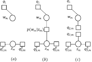
Figure 2: EP steps for updating $q_{2,m}(w_{m},z_{m})$: $(a)$ Eliminate $q_{2,m}(w_{m},z_{m})$ from the factor graph to find the cavity distribution $Q_{\backslash 2m}(w_{m},z_{m})$ as in (28), $(b)$ Use $p(w_{m}|z_{m})$ factor to define the hybrid posterior distribution $R_{2,m}(w_{m},z_{m})$ as in (32), and $(c)$ Project $R_{2,m}(w_{m},z_{m})$ onto $\mathcal{F}$ and update $q_{2,m}(w_{m},z_{m})$ as in (34), (III), and (48).

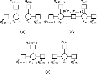
Figure 3: EP steps for updating $q^{R}_{3,m-1}(z_{m-1})$ and $q^{F}_{3,m}(z_{m})$: $(a)$ Eliminate $q^{R}_{3,m-1}(z_{m-1})$ and $q^{F}_{3,m}(z_{m})$ from the factor graph to find the cavity distributions $q^{\backslash R}_{3,m-1}(z_{m-1})$ and $q^{\backslash F}_{3,m}(z_{m})$ as in (51) and (54), $(b)$ Use $p(z_{m}|z_{m-1})$ factor to define the hybrid posterior distribution $S_{3,m-1,m}(z_{m-1},z_{m})$ as in (56), and $(c)$ Project $S_{3,m-1,m}(z_{m-1},z_{m})$ onto $\mathcal{F}$ and update $q^{R}_{3,m-1}(z_{m-1})$ and $q^{F}_{3,m}(z_{m})$ as in (62)-(65).

Now as $q_{1}(\mathbf{w})$ approximates $p(\mathbf{y}|\bm{\Phi}(\bm{\theta}),\mathbf{w},\eta)$ which is a complex Gaussian function of $\mathbf{w}$ then to simplify we set $q_{1}(\mathbf{w})\propto\mathcal{CN}(\mathbf{y};\bm{\Phi}\mathbf{w},\eta^{-1}\mathbf{I}_{N})$. Expanding this Gaussian distribution and completing the square for $\mathbf{w}$, we get

$$\bm{\Sigma}^{-1}_{1}=\eta\bm{\Phi}^{H}\bm{\Phi},\quad\bm{\Sigma}^{-1}_{1}\bm{\mu}_{1}=\eta\bm{\Phi}^{H}\mathbf{y},$$ (24)

using (24), (21) and (22) can be simplified as

$$\bm{\Sigma} =\bm{\Sigma}_{2}-\bm{\Sigma}_{2}\bm{\Phi}^{H}\left(\eta^{-1}\mathbf{I}_{N}+\bm{\Phi}\bm{\Sigma}_{2}\bm{\Phi}^{H}\right)^{-1}\bm{\Phi}\bm{\Sigma}_{2},$$ (25)

$$\bm{\mu} =\bm{\Sigma}\left(\eta\bm{\Phi}^{H}\mathbf{y}+\bm{\Sigma}^{-1}_{2}\bm{\mu}_{2}\right),$$ (26)

Thus to compute (23), (25), and (26) we just need to update the approximation factors $q_{2}(\mathbf{w},\mathbf{z})$ and $q_{3}(\mathbf{z})$. We first update $q_{2}(\mathbf{w},\mathbf{z})$ as follow. Since it is equal to the product of marginals $q_{2,m}(w_{m},z_{m})$, we can instead update each marginal distribution individually and in parallel [26]. The steps involved in upating $q_{2,m}(w_{m},z_{m})$ are depicted in Fig. 2. Let $Q_{m}(w_{m},z_{m})$ denote the marginal distribution obtained from (13). Then using (14) and (15) we can write

$$Q_{m}(w_{m},z_{m}) =Q_{m}(w_{m})Q_{m}(z_{m}),$$

$$\propto\mathcal{CN}(w_{m};\mu_{m},\Sigma_{m,m})\text{Bern}(z_{m};\sigma(p_{m})),$$ (27)

where $\mu_{m}$ is the $m$-th element of $\bm{\mu}$, and $\Sigma_{m,m}=[\bm{\Sigma}]_{m,m}$, $m=1,2,\ldots,M$. Following the EP framework we first find the cavity distribution as

$$Q_{\backslash 2,m}(w_{m},z_{m}) =\frac{Q_{m}(w_{m},z_{m})}{q_{2,m}(w_{m},z_{m})}\propto Q_{\backslash 2,m}(w_{m})Q_{\backslash 2,m}(z_{m}),$$ (28)

where $Q_{\backslash 2,m}(w_{m})=\mathcal{CN}(w_{m};\mu_{\backslash 2,m},\Sigma_{\backslash 2,m})$ and $Q_{\backslash 2,m}(z_{m})=\text{Bern}(z_{m};\sigma(p_{\backslash 2,m}))$. The parameters in these distributions are given by

$$\Sigma_{\backslash 2,m} =\left(\Sigma^{-1}_{m,m}-\Sigma^{-1}_{2,m}\right)^{-1},$$ (29)

$$\mu_{\backslash 2,m} =\Sigma_{\backslash 2,m}\left(\Sigma^{-1}_{m,m}\mu_{m}-\Sigma^{-1}_{2,m}\mu_{2,m}\right),$$ (30)

$$p_{\backslash 2,m} =p_{m}-p_{2,m},$$ (31)

Next we define the hybrid posterior distribution $R_{2,m}(w_{m},z_{m})$ as

$$R_{2,m}(w_{m},z_{m}) =\frac{1}{C_{m}}p(w_{m}|z_{m})Q_{\backslash 2,m}(w_{m},z_{m}),$$ (32)

where $p(w_{m}|z_{m})$ is defined in (6). The normalization constant $C_{m}$ in (32) is computed as follow

$$C_{m} =\sum_{z_{m}\in\{0,1\}}\int p(w_{m}|z_{m})Q_{\backslash 2,m}(w_{m},z_{m})d{w_{m}},$$

$$=\int\mathcal{CN}(w_{m};0,\gamma^{-1}_{m})\mathcal{CN}(w_{m};\mu_{\backslash 2,m},\Sigma_{\backslash 2,m})dw_{m}\sigma(p_{\backslash 2,m})$$

$$\quad+\int\delta(w_{m})\mathcal{CN}(w_{m};\mu_{\backslash 2,m},\Sigma_{\backslash 2,m})dw_{m}(1-\sigma(p_{\backslash 2,m})),$$

$$=\mathcal{CN}(0;\mu_{\backslash 2,m},\Sigma_{\backslash 2,m}+\gamma^{-1}_{m})\sigma(p_{\backslash 2,m})+\mathcal{CN}(0;\mu_{\backslash 2,m},\Sigma_{\backslash 2,m})(1-\sigma(p_{\backslash 2,m})),$$ (33)

We now update the approximation $Q_{m}(w_{m},z_{m})$ by projecting $R_{2,m}(w_{m},z_{m})$ onto the closest distribution in $\mathcal{F}$ by minimizing the following Kullback-Leibler (KL) divergence

$$Q_{m}(w_{m},z_{m})=\operatorname*{arg\,min}_{Q_{m}(w_{m},z_{m})\in\mathcal{F}}KL(R_{2,m}(w_{m},z_{m})\|Q_{m}(w_{m},z_{m})),$$ (34)

since $Q_{m}(w_{m},z_{m})=Q_{m}(w_{m})Q_{m}(z_{m})$ from (III), it can be shown that the optimization problem in (34) is equivalent to solving the following two separate problems [30]

$$Q_{m}(w_{m}) =\operatorname*{arg\,min}_{Q_{m}(w_{m})\in\mathcal{F}}KL\left(R_{2,m}(w_{m})\|Q_{m}(w_{m})\right),$$ (35)

and

$$Q_{m}(z_{m}) =\operatorname*{arg\,min}_{Q_{m}(z_{m})\in\mathcal{F}}KL\left(R_{2,m}(z_{m})\|Q_{m}(z_{m})\right),$$ (36)

where $R_{2,m}(w_{m})$ and $R_{2,m}(z_{m})$ are the marginal distributions of $R_{2,m}(z_{m})$. The KL divergence in (35) and (36) is minimized by using the moment matching property [33]. Thus for $Q_{m}(w_{m})$ and $Q_{m}(z_{m})$ defined in (III) we set

$$\mu_{m} =\mathbb{E}_{R_{2,m}}[w_{m}],$$ (37)

$$\Sigma_{m,m} =\mathbb{E}_{R_{2,m}}[\lvert w_{m}\rvert^{2}]-\lvert\mathbb{E}_{R_{2,m}}[w_{m}]\rvert^{2},$$ (38)

$$\sigma(p_{m}) =\mathbb{E}_{R_{2,m}}[z_{m}],$$ (39)

The values of $\mu_{m}$, $\Sigma_{m,m}$, and $\sigma(p_{m})$ are given in the following lemma which is proved in Appendix A.

Lemma 1.

1. The posterior mean value $\sigma(p_{m})$ is given by

   $$\sigma(p_{m})=\left(1+\frac{\sigma(-p_{\backslash 2,m})\mathcal{CN}(0;\mu_{\backslash 2,m},\Sigma_{\backslash 2,m})}{\sigma(p_{\backslash 2,m})\mathcal{CN}(0;\mu_{\backslash 2,m},\Sigma_{\backslash 2,m}+\gamma^{-1}_{m})}\right)^{-1},$$ (40)

2. The posterior mean value $\mu_{m}$ is given by

   $$\mu_{m}=\mu_{\backslash 2,m}+\Sigma_{\backslash 2,m}\frac{\partial\ln C_{m}}{\partial\mu^{*}_{\backslash 2,m}},$$ (41)

   where

   $$\frac{\partial\ln C_{m}}{\partial\mu_{\backslash 2,m}}=-\sigma(p_{m})\frac{\mu^{*}_{\backslash 2,m}}{\Sigma_{\backslash 2,m}+\gamma^{-1}_{m}}-\sigma(-p_{m})\frac{\mu^{*}_{\backslash 2,m}}{\Sigma_{\backslash 2,m}},$$ (42)

3. The posterior variance $\Sigma_{m,m}$ is given by

   $$\Sigma_{m,m}=\Sigma_{\backslash 2,m}+(\Sigma_{\backslash 2,m})^{2}\left[\frac{\partial\ln C_{m}}{\partial\Sigma_{\backslash 2,m}}-\frac{\partial\ln C_{m}}{\partial\mu^{*}_{\backslash 2,m}}\frac{\partial\ln C_{m}}{\partial\mu_{\backslash 2,m}}\right],$$ (43)

   where

   $$\frac{\partial\ln C_{m}}{\partial\Sigma_{\backslash 2,m}}=\sigma(p_{m})\frac{|\mu_{\backslash 2,m}|^{2}-\left(\Sigma_{\backslash 2,m}+\gamma^{-1}_{m}\right)}{\left(\Sigma_{\backslash 2,m}+\gamma^{-1}_{m}\right)^{2}}+\sigma(-p_{m})\frac{|\mu_{\backslash 2,m}|^{2}-\left(\Sigma_{\backslash 2,m}\right)}{\left(\Sigma_{\backslash 2,m}\right)^{2}},$$ (44)

Next we update the factor $q_{2,m}(w_{m},z_{m})$. Since $q_{2,m}(w_{m},z_{m})$$=q_{2,m}(w_{m})q_{2,m}(z_{m})$ we can update the marginals separately. To update $q_{2,m}(w_{m})$ we write

$$q_{2,m}(w_{m}) =\frac{Q_{m}(w_{m})}{Q_{\backslash 2,m}(w_{m})}=\frac{\mathcal{CN}(w_{m};\mu_{m},\Sigma_{m,m})}{\mathcal{CN}(w_{m};\mu_{\backslash 2,m},\Sigma_{\backslash 2,m})},$$

$$\propto\mathcal{CN}(w_{m};\mu_{2,m},\Sigma_{2,m}),$$ (45)

where

$$\Sigma_{2,m} =\left(\left(\Sigma_{m,m}\right)^{-1}-\left(\Sigma_{\backslash 2,m}\right)^{-1}\right)^{-1},$$ (46)

$$\mu_{2,m} =\Sigma_{2,m}\left(\left(\Sigma_{m,m}\right)^{-1}\mu_{m}-\left(\Sigma_{\backslash 2,m}\right)^{-1}\mu_{\backslash 2,m}\right),$$ (47)

and to update $q_{2,m}(z_{m})$ we write

$$q_{2,m}(z_{m}) =\frac{Q_{m}(z_{m})}{Q_{\backslash 2,m}(z_{m})}=\frac{\text{Bern}(z_{m};\sigma(p_{m}))}{\text{Bern}(z_{m};\sigma(p_{\backslash 2,m}))}\propto\text{Bern}(z_{m};\sigma(p_{2,m})),$$ (48)

where

$$\sigma(p_{2,m})=\frac{\mathcal{CN}(0;\mu_{\backslash 2,m},\Sigma_{\backslash 2,m}+\gamma^{-1}_{m})}{\mathcal{CN}(0;\mu_{\backslash 2,m},\Sigma_{\backslash 2,m}+\gamma^{-1}_{m})+\mathcal{CN}(0;\mu_{\backslash 2,m},\Sigma_{\backslash 2,m})},$$ (49)

and using the logit function $\sigma^{-1}(.)$ on (49) we get

$$p_{2,m}=\ln\mathcal{CN}(0;\mu_{\backslash 2,m},\Sigma_{\backslash 2,m}+\gamma^{-1}_{m})-\ln\mathcal{CN}(0;\mu_{\backslash 2,m},\Sigma_{\backslash 2,m})$$ (50)

Next we update the approximation factor $q_{3}(\mathbf{z})$ in (20). We start by updating $q^{R}_{3,m-1}(z_{m-1})$ and $q^{F}_{3,m}(z_{m})$. The EP steps taken to update these factors are summarized in Fig. 3. Given the marginal distribution on $z_{m}$ as $Q_{m}(z_{m})=q^{F}_{3,m}(z_{m})q_{2,m}(z_{m})q^{R}_{3,m}(z_{m})$ which is also easily observable from Fig. 1(b), we first find the cavity distribution $q^{\backslash R}_{3,m-1}(z_{m-1})$ as follow

$$q^{\backslash R}_{3,m-1}(z_{m-1}) =\frac{Q_{m-1}(z_{m-1})}{q^{R}_{3,m-1}(z_{m-1})}=q^{F}_{3,{m-1}}(z_{m-1})q_{2,{m-1}}(z_{m-1})$$

$$\propto\text{Bern}\left(z_{m-1};\sigma\left(p^{\backslash R}_{3,m-1}\right)\right),$$ (51)

where

$$\sigma\left(p^{\backslash R}_{3,m-1}\right)=\frac{\sigma\left(p^{F}_{3,m-1}\right)\sigma\left(p_{2,m-1}\right)}{\sigma\left(p^{F}_{3,m-1}\right)\sigma\left(p_{2,m-1}\right)+\sigma\left(-p^{F}_{3,m-1}\right)\sigma\left(-p_{2,m-1}\right)},$$ (52)

Solving (52) using the logit function $\sigma^{-1}(.)$ and adjusting the notation to update the $m$-th factor we get

$$p^{\backslash R}_{3,m} =p_{2,m}+p^{F}_{3,m},\quad\text{for}\ m=1,2,\ldots,M-1$$ (53)

Similarly, the cavity distribution $q^{\backslash F}_{3,m}(z_{m})$ can also be found by

$$q^{\backslash F}_{3,m}(z_{m})=\frac{Q_{m}(z_{m})}{q^{F}_{3,m}(z_{m})}=q^{R}_{3,m}(z_{m})q_{2,m}(z_{m})\propto\text{Bern}\left(z_{m};\sigma\left(p^{\backslash F}_{3,m}\right)\right).$$ (54)

Following a similar approach as in (52) and (53) we get

$$p^{\backslash F}_{3,m} =\left\{\begin{matrix}&p_{2,m}+p^{R}_{3,m},&&\text{for}\quad m=1,2,\ldots,M-1\\ &p_{2,m},&&\text{for}\quad m=M\end{matrix}\right.$$ (55)

Once the cavity distributions are computed, we define the hybrid joint posterior distribution on $z_{m-1}$ and $z_{m}$ as

$$S_{3,m-1,m}(z_{m-1},z_{m}) =q^{\backslash R}_{3,m-1}(z_{m-1})p(z_{m}|z_{m-1})q^{\backslash F}_{3,m}(z_{m}),$$ (56)

in which $p(z_{m}|z_{m-1})$ is given in (II). Since (56) involves a product of Bernoulli distributions, $S_{3,m-1,m}(z_{m-1},z_{m})$ is a bivariate Bernoulli distribution where the marginal distributions on $z_{m-1}$ and $z_{m}$ can be written as

$$S_{3,m-1}(z_{m-1}) =\sum_{z_{m}\in\{0,1\}}S_{3,m-1,m}(z_{m-1},z_{m}),$$ (57)

$$S_{3,m}(z_{m}) =\sum_{z_{m-1}\in\{0,1\}}S_{3,m-1,m}(z_{m-1},z_{m}),$$ (58)

and using their derived forms in Appendix B the means of these marginal Bernoulli distributions are found as

$$\mathbb{E}_{S_{3,m-1}}[z_{m-1}]=\frac{1}{D_{m}}\sigma(p^{\backslash R}_{3,m-1})\left[\sigma(p^{\backslash F}_{3,m})(1-\tau_{10})+\sigma(-p^{\backslash F}_{3,m})\tau_{10}\right],$$ (59)

$$\mathbb{E}_{S_{3,m}}[z_{m}]=\frac{1}{D_{m}}\sigma(p^{\backslash F}_{3,m})\left[\sigma(p^{\backslash R}_{3,m-1})(1-\tau_{10})+\sigma(-p^{\backslash R}_{3,m-1})\tau_{01}\right],$$ (60)

where the normalization constant $D_{m}$ is given by

$$D_{m} =\sigma(-p^{\backslash R}_{3,m-1})\sigma(-p^{\backslash F}_{3,m})(1-\tau_{01})+\sigma(p^{\backslash R}_{3,m-1})\sigma(-p^{\backslash F}_{3,m})\tau_{10}$$

$$+\sigma(-p^{\backslash R}_{3,m-1})\sigma(p^{\backslash F}_{3,m})\tau_{01}+\sigma(p^{\backslash R}_{3,m-1})\sigma(p^{\backslash F}_{3,m})(1-\tau_{10}),$$ (61)

Now we update the approximation factors $Q_{m-1}(z_{m-1})$ and $Q_{m}(z_{m})$ by projecting
$S_{3,m-1,m}(z_{m-1},z_{m})$ in (56) onto the closest distribution in $\mathcal{F}$. This is done by minimizing the KL divergence between $S_{3,m-1,m}(z_{m-1},z_{m})$ and $Q_{m-1}(z_{m-1})Q_{m}(z_{m})$. As in (34), this can be achieved by solving two separate optimization problems

$$Q_{m-1}(z_{m-1})=\operatorname*{arg\,min}_{Q_{m-1}(z_{m-1})\in\mathcal{F}}KL\left(S_{3,m-1}(z_{m-1})\|Q_{m-1}(z_{m-1})\right),$$ (62)

and

$$Q_{m}(z_{m}) =\operatorname*{arg\,min}_{Q_{m}(z_{m})\in\mathcal{F}}KL\left(S_{3,m}(z_{m})\|Q_{m}(z_{m})\right),$$ (63)

where the marginals $S_{3,m-1}(z_{m-1})$ and $S_{3,m}(z_{m})$ are computed from (57) and (58). The KL divergence in (62) and (63) is minimized as before by using the moment matching property. Thus we set $\sigma(p_{m-1})=\mathbb{E}_{S_{3,m-1}}[z_{m-1}]$ given in (59) and $\sigma(p_{m})=\mathbb{E}_{S_{3,m}}[z_{m}]$ given in (60).

Finally we update the approximation factors $q^{R}_{3,m-1}(z_{m-1})$ and $q^{F}_{3,m}(z_{m})$ as follow. To update $q^{R}_{3,m-1}(z_{m-1})$ we write

$$q^{R}_{3,m-1}(z_{m-1})=\frac{Q_{m-1}(z_{m-1})}{q^{\backslash R}_{3,m-1}(z_{m-1})}\propto\text{Bern}(z_{m-1};\sigma(p^{R}_{3,m-1})),$$ (64)

where $\sigma(p^{R}_{3,m-1})$ is computed from (66) in which the notation is adjusted to compute the $m$-th factor. Similarly to update $q^{F}_{3,m}(z_{m})$ we write

$$q^{F}_{3,m}(z_{m})=\frac{Q_{m}(z_{m})}{q^{\backslash F}_{3,m}(z_{m})}\propto\text{Bern}(z_{m};\sigma(p^{F}_{3,m})),$$ (65)

where $\sigma(p^{F}_{3,m})$ is computed from (67). This completes all the posterior updates required for an EP’s iteration. The complete EP algorithm is summarized in Algorithm 1.

Input: $\mathbf{y}$

Parameters: $\bm{\xi}$,$\bm{\theta}$.

/* EP run */

for each $n=\{1,2,\ldots,n_{EP}\}$ 

1.  

   Compute $Q(\mathbf{w},\mathbf{z})$ parameters $\mathbf{p}$, $\bm{\Sigma}$, and $\bm{\mu}$ using (23), (25),

       and (26), respectively. /* Updating factor $q_{2}(\mathbf{w},\mathbf{z})$: */

       for each $m=\{1,2,\ldots,M\}$ 

1.        

   Find $Q_{\backslash 2,m}(w_{m},z_{m})$ parameters $\Sigma_{\backslash 2,m}$, $\mu_{\backslash 2,m}$, and

$p_{\backslash 2,m}$ from (29), (30), and (31), respectively.

       

Update $Q_{m}(w_{m},z_{m})$ by computing $p_{m}$ from (40),

$\mu_{m}$ from (41), and $\Sigma_{m,m}$ using (43).

       

Update the factor $q_{2,m}(w_{m},z_{m})$ by computing $\Sigma_{2,m}$

             from (46), $\mu_{2,m}$ from (47), and $p_{2,m}$ using (50).

       end

      /* Updating factor $q_{3}(\mathbf{z})$: */

       /* Forward pass: */

       for each $m=\{1,2,\ldots,M\}$ 

1.        

   To update $q^{\backslash R}_{3,m}(z_{m})$ factor, compute $p^{\backslash R}_{3,m}$ from (53),

if $m<M$.

       

Update $q^{F}_{3,m}(z_{m})$ by computing $p^{F}_{3,m}$ using (67),

             if $m>1$.

       end

      /* Reverse pass: */

       for each $m=\{M,M-1,\ldots,1\}$ 

1. To update $q^{\backslash F}_{3,m}(z_{m})$ factor, compute $p^{\backslash F}_{3,m}$ from (55).

2.        

   Update the factor $q^{R}_{3,m}(z_{m})$ by computing $p^{R}_{3,m}$ from

             (66), if $m<M$.

       end

      /* Check for convergence: Keep track of $\bm{\mu}$ for each $n^{th}$ iteration */

       if $\frac{||\bm{\mu}^{n}-\bm{\mu}^{n-1}||}{||\bm{\mu}^{n-1}||}<\epsilon_{EP}$ then

            break;

       end if

      

end

Output: $\bm{\mu}$, $\bm{\Sigma}$, $\mathbf{p}$

Algorithm 1 EP Algorithm

$$\sigma(p^{R}_{3,m}) =\frac{\sigma\left(p^{\backslash F}_{3,m+1}\right)(1-\tau_{10})+\sigma\left(-p^{\backslash F}_{3,m+1}\right)\tau_{10}}{\sigma\left(p^{\backslash F}_{3,m+1}\right)(1-\tau_{10})+\sigma\left(-p^{\backslash F}_{3,m+1}\right)\tau_{10}+\sigma\left(p^{\backslash F}_{3,m+1}\right)\tau_{01}+\sigma\left(-p^{\backslash F}_{3,m+1}\right)(1-\tau_{01})},$$

$$~{}~{}~{}~{}\text{for }~{}m=1,2,\ldots,M-1,$$ (66)

$$\sigma(p^{F}_{3,m}) =\sigma\left(p^{\backslash R}_{3,m-1}\right)(1-\tau_{10})+\sigma\left(-p^{\backslash R}_{3,m-1}\right)\tau_{01},\qquad\text{for }m=2,\ldots,M,$$ (67)

Remark 1.

In order to improve the convergence of our proposed EP algorithm, when $\big{(}\left(\Sigma_{m,m}\right)^{-1}\\ -\left(\Sigma_{\backslash 2,m}\right)^{-1}\big{)}^{-1}\geq 0$, we follow the approach suggested in [33, 26] for an EP algorithm, and damp the updates of the factors $\{q_{2,m}(w_{m},z_{m})\}^{M}_{m=1}$, $\{q^{F}_{3,m}(z_{m})\}^{M}_{m=2}$, and $\{q^{R}_{3,m}(z_{m})\}^{M-1}_{m=1}$ in every EP iteration. Using a smoothing mechanism the parameters $\Sigma_{2,m},~{}\mu_{2,m},~{}p_{2,m}$ and $p^{j}_{3,m}$, $j\in\{F,R\}$, are damped according to the equation

$$\psi^{damp}=\beta\psi+(1-\beta)\psi^{old}$$ (68)

where $\beta\in(0,1)$ is the smoothing factor, $\psi^{old}$ represents the parameter in the previous EP iteration and $\psi$ is the value calculated according to the dervations in Section III. The superscript $damp$ denotes the value of the parameter after applying the smoothing mechanism. The above damped updates replace the respective undamped ones in the next iteration of EP. Further, to improve the convergence of EP we use the annealed damping scheme as suggested in [33] where we start the EP algorithm with $\beta=0.5$ and progressively anneal its value by multiplying it with a constant $\kappa<1$ after every iteration of EP until convergence. Based on empirical evidence we select $\kappa=0.945$ for the considered channel estimation problem in this paper. Note that as indicated in [33] we can also have $\left(\left(\Sigma_{m,m}\right)^{-1}-\left(\Sigma_{\backslash 2,m}\right)^{-1}\right)^{-1}<0$ and when this happen we just set $\Sigma_{2,m}=10^{2}$ and use the above smoothing mechanism.

IV Expectation Maximization algorithm: E-step and M-step derivations

In this section we evaluate the E-Step and M-step of the EM algorithm as discussed in (11) and (12). Using EM we aim to iteratively find the ML estimate of the unknown parameters $\bm{\xi}=(\bm{\tau},\gamma_{1},\gamma_{2},\ldots,\gamma_{M},\eta,\bm{\theta})^{T}$. For the complete data defined in section II as $\mathbf{d}=[\mathbf{y}^{T},\mathbf{w}^{T},\mathbf{z}^{T}]^{T}$ and using the EP’s approximation to the posterior distribution from (13), the E-step in (11) can be written as

$${\mathcal{L}}(\bm{\xi};\bm{\xi}^{l})\approx\mathbb{E}_{Q(\mathbf{w},\mathbf{z}|\mathbf{y},\bm{\xi}^{l})}\left[\ln p(\mathbf{y},\mathbf{w},\mathbf{z}|\bm{\xi})\right],$$

$$=\mathbb{E}_{Q(\mathbf{w},\mathbf{z}|\mathbf{y},\bm{\xi}^{l})}\left[\ln p(\mathbf{y}|\bm{\Phi}(\bm{\theta}),\mathbf{w},{\eta})p(\mathbf{w}|\mathbf{z},{\bm{\gamma}})p(\mathbf{z}|{p}_{10},{p}_{01})\right],$$ (69)

Since jointly maximizing (IV) over $\bm{\xi}$ is difficult, here we instead update $\bm{\xi}$ one element at a time while keeping the other elements fixed to their current estimates in the $l$-th iteration [43]. To estimate $\tau_{10}$ and $\tau_{01}$, since only $p(\mathbf{z}|\bm{\tau})$ involves these parameters, (IV) simplifies to

$${\mathcal{L}}_{1}(\bm{\tau};\bm{\tau}^{l})=\mathbb{E}_{Q(\mathbf{w},\mathbf{z}|\mathbf{y},\bm{\xi}^{l})}\left[\ln p(\mathbf{z}|{p}_{10},{p}_{01})\right]$$

$$=\sum^{M}_{m=2}\left[\ln(1-\tau_{01})+\sigma\left(p^{(l+1)}_{m}\right)\sigma\left(p^{(l+1)}_{m-1}\right)\times\right.\left.\ln\frac{(1-\tau_{10})(1-\tau_{01})}{\tau_{01}\tau_{10}}+\sigma\left(p^{(l+1)}_{m}\right)\ln\frac{\tau_{01}}{(1-\tau_{01})}\right.$$

$$\left.+\sigma\left(p^{(l+1)}_{m-1}\right)\ln\frac{\tau_{10}}{(1-\tau_{01})}\right]+\text{const},$$ (70)

where we use the fact that $\mathbb{E}_{Q}[z_{m}]=\sigma(p_{m})$. Maximizing ${\mathcal{L}}_{1}(.)$ with respect to (w.r.t) $\bm{\tau}$, we get the update equations as

$$\tau^{(l+1)}_{01} =\frac{\sum^{M}_{m=2}\left[\sigma\left(p^{(l+1)}_{m-1}\right)\left(1-\sigma\left(p^{(l+1)}_{m}\right)\right)\right]}{\sum^{M}_{m=2}\sigma\left(p^{(l+1)}_{m-1}\right)},$$ (71)

$$\tau^{(l+1)}_{10} =\frac{\sum^{M}_{m=2}\left[\sigma\left(p^{(l+1)}_{m}\right)\left(1-\sigma\left(p^{(l+1)}_{m-1}\right)\right)\right]}{\sum^{M}_{m=2}\left(1-\sigma\left(p^{(l+1)}_{m-1}\right)\right)},$$ (72)

Similarly, maximizing ${\mathcal{L}}(.)$ w.r.t $\gamma_{m}$ and $\eta$ we get

$$\gamma^{(l+1)}_{m}=\left(\Sigma^{(l+1)}_{m,m}+|\mu^{(l+1)}_{m}|^{2}\right)^{-1},$$ (73)

and,

$$\eta^{(l+1)}=\frac{N}{\|\mathbf{y}-\bm{\Phi}(\bm{\theta}^{l})\bm{\mu}^{(l+1)}\|^{2}+\text{tr}\left\{\bm{\Phi}(\bm{\theta}^{l})\bm{\Sigma}^{(l+1)}\bm{\Phi}^{H}(\bm{\theta}^{l})\right\}},$$ (74)

where to get (73) we use the fact that $\mathbb{E}_{Q}[|w_{m}|^{2}]=\Sigma_{m,m}+|\mu_{m}|^{2}$ in which $\mu_{m}$ and $\Sigma_{m,m}$ are defined in (III), and in (74) we use the fact that $\mathbb{E}_{Q}[\mathbf{w}]=\bm{\mu}$ and $\mathbb{E}_{Q}[\mathbf{w}\mathbf{w}^{H}]=\bm{\Sigma}+\bm{\mu}\bm{\mu}^{H}$. Both $\bm{\Sigma}$ and $\bm{\mu}$ are given in (25) and (26).

Finally to update $\bm{\theta}$ for dictionary learning and minimizing the modeling error, the objective function in (IV) can be simplified to

$${\mathcal{L}}_{2}(\bm{\theta})=\|\mathbf{y}-\bm{\Phi}(\bm{\theta})\bm{\mu}^{(l+1)}\|^{2}+\text{tr}\left\{\bm{\Phi}(\bm{\theta})\bm{\Sigma}^{(l+1)}\bm{\Phi}(\bm{\theta})^{H}\right\},$$ (75)

As seen from (75), a closed-form update equation for $\bm{\theta}$ can not be obtained, but we can use numerical methods, for instance, gradient descent (GD) to update $\bm{\theta}$ in the $l$-th iteration. However, GD employs backtracking line search [44] to adaptively select the step-size which requires constant evaluation of the objective function in (75). Thus, to reduce the computational complexity we adopt the following single-step update for $\bm{\theta}$ with a constant step-size as suggested in [17, 20], i.e.,

$$\bm{\theta}^{(l+1)}=\bm{\theta}^{l}-\frac{r_{\theta}}{100}\text{sign}\left\{\nabla_{\bm{\theta}^{l}}{\mathcal{L}}_{2}\left(\bm{\theta}^{l}\right)\right\},$$ (76)

where $r_{\theta}$ is the grid interval, and sign{.} represent the signum function which has negligible computational complexity. The step size $r_{\theta}/100$ divides the grid interval into $100$ equal parts, thus in the worst case the true values may be obtained in less than $100$ iterations. Further, this step size ensures that the final direction mismatch error is less than $1\%$ of $r_{\theta}$ which for sufficiently small $r_{\theta}$ is negligible to have significant impact on the channel estimation error.

The $m^{th}$ term of the gradient $\nabla_{\bm{\theta}}{\mathcal{L}}_{2}(\bm{\theta})$ is given by

$$\left[\nabla_{\bm{\theta}^{l}}{\mathcal{L}}_{2}\left(\bm{\theta}^{l}\right)\right]_{m}=\frac{\partial}{\partial\theta^{l}_{m}}{\mathcal{L}}_{2}\left(\bm{\theta}^{l}\right)$$

$$=2\alpha^{(l+1)}_{1}\Re\{\dot{\mathbf{a}}^{H}(\theta^{l}_{m})\mathbf{X}^{H}\mathbf{X}{\mathbf{a}}(\theta^{l}_{m})\}+2\Re\{\dot{\mathbf{a}}^{H}(\theta^{l}_{m})\mathbf{X}^{H}\bm{\alpha}^{(l+1)}_{2}\},$$ (77)

in which, $\alpha^{(l+1)}_{1}=|\mu^{(l+1)}_{m}|^{2}+\Sigma^{(l+1)}_{m,m}$, $\bm{\alpha}^{(l+1)}_{2}=\mathbf{X}\sum_{n\neq m}\Sigma^{(l+1)}_{n,m}\mathbf{a}(\theta^{l}_{n})-\mathbf{y}^{(l+1)}_{\backslash m}\left(\mu^{(l+1)}_{m}\right)^{*}$, and $\mathbf{y}^{(l+1)}_{\backslash m}=\mathbf{y}-\mathbf{X}\sum_{n\neq m}(\mu^{(l+1)}_{n}\mathbf{a}(\theta^{l}_{n}))$. The scalar $\Sigma^{(l+1)}_{n,m}=\left[\bm{\Sigma}^{(l+1)}\right]_{n,m}$ and the vector $\dot{\mathbf{a}}(\theta^{l}_{m})=\frac{\partial}{\partial\theta^{l}_{m}}\mathbf{a}(\theta^{l})$ is computed from (2) for $m=1,2,\ldots,M$.

This completes all the sequential updates required to estimate $\bm{\xi}$ in the $(l+1)$-st iteration. The parameters in $\bm{\xi}$ are repeatedly updated in the EM iterations until convergence. The overall EM-EP algorithm is summarized in Algorithm 2.

Input: $\mathbf{y}$

Parameters: $\bm{\xi}^{(0)}$,$\bm{\theta}^{(0)}$, $\mu_{2,m}=0$, $\Sigma_{2,m}=10^{2}$, $p_{2,m}=0$, $p^{F}_{3,m}=0$ for $m=2,\ldots,M$, $p^{R}_{3,m}=0$ for $m=1,2,\ldots,M-1$.

/* EM-EP run */

for each $l=\{0,1,2,\ldots,n_{EM}-1\}$ 

1.  

   Given $\bm{\xi}^{l}$ and $\bm{\theta}^{l}$ run the EP algorithm described in

Algorithm 1 to generate $\bm{\mu}^{(l+1)}$, $\bm{\Sigma}^{(l+1)}$, and $\mathbf{p}^{(l+1)}$.

 

Check for convergence:

       if $\frac{||\bm{\mu}^{(l+1)}-\bm{\mu}^{l}||}{||\bm{\mu}^{l}||}<\epsilon_{EM}$ then

             break;

       end if

 

Use $\bm{\mu}^{(l+1)}$, $\bm{\Sigma}^{(l+1)}$, and $\mathbf{p}^{(l+1)}$ to update $\tau_{10}$, $\tau_{01}$,

       $\bm{\gamma}$, $\eta$, and $\bm{\theta}$ using (71), (72), (73), (74), and (76), respectively.

end

Output: $\hat{\mathbf{h}}=\mathbf{A}(\bm{\theta}^{(l+1)})\bm{\mu}^{(l+1)}$

Algorithm 2 Overall EM-EP Algorithm

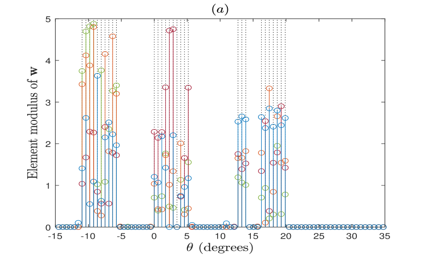
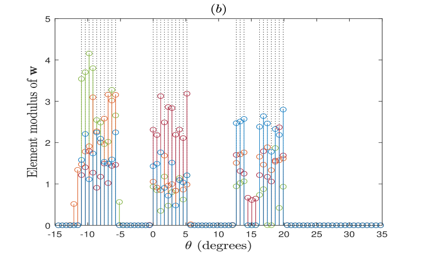
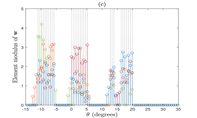
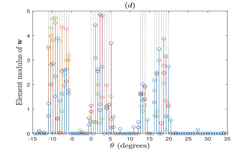
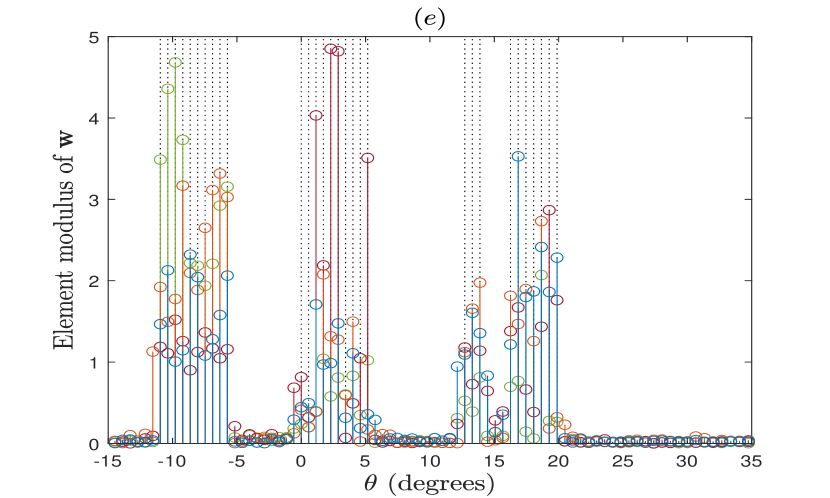
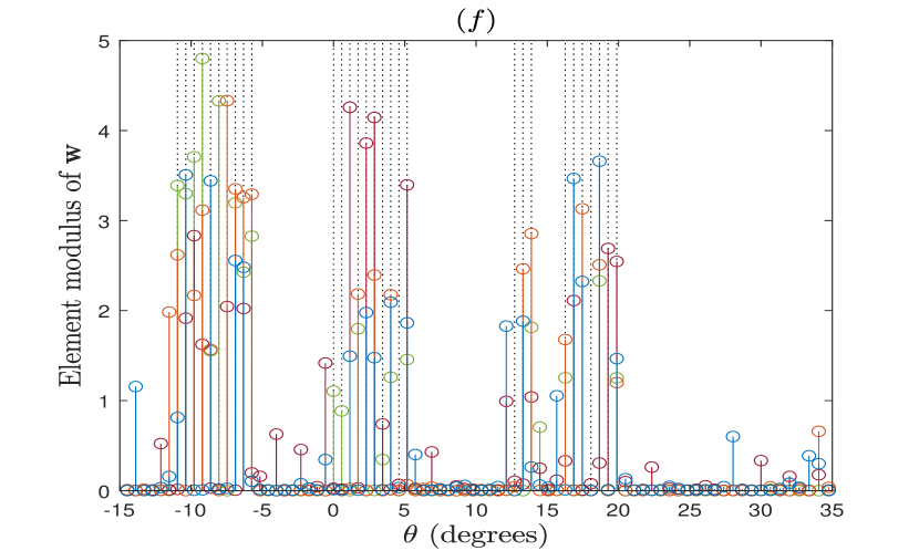
Figure 4: Magnitude of the elements in $\mathbf{w}$ for four independent trials with $G=128$, $M=200$, $N=48$, $L_{s}=3$, $L_{p}=10$, and $SNR=10$ dB, and for $(a)$ EM-EP, $(b)$ SuRe-CSBL, $(c)$ S-TCS, $(d)$ EM-EP-B, $(e)$ PC-VB, $(f)$ EM-BG-GAMP. The dotted lines indicate locations of the true AoDs.

IV-A Computational Complexity of EM-EP algorithm

The computational complexity of the proposed EP algorithm per iteration is dominated by (25) and (26) which can be solved in $O(NM^{2})$ computations. This complexity is the same as that of the EP algorithm proposed in [33]. For the EM part of the algorithm, the dominant terms include the update of $\eta$ by (74) which takes $O(NM^{2})$ computations, and the update of $\bm{\theta}$ by (76) which takes $O(GNM)$ computations. Since $M$ is usually greater than $G$, the complexity of the proposed EM-EP algorithm is $O(NM^{2})$ per iteration which is the same as that of the off-grid SBL algorithm proposed in [17].

V Simulation Results

In this section, we investigate the performance of the proposed EM-EP algorithm for massive MIMO channel estimation. We consider a single-cell where a BS equipped with a ULA has $G$ antennas and transmits $N$ pilot symbols to a reference user. The elements in the pilot matrix $\mathbf{X}$ are selected from a circularly symmetric complex Gaussian distribution with unit variance, and the DL channel $\mathbf{h}$ between the BS and the user is generated using the $3$GPP spatial channel model [45] with urban-micro cell environment. We assume that each channel realization is composed of $L_{s}$ scatterers with AoDs randomly located in the interval $[-90^{\text{o}},90^{\text{o}}]$, and each scatterer has $L_{p}$ paths with the AoDs randomly generated and concentrated in an angular spread denoted by $A$. Unless stated otherwise, the AoDs of all the paths in a channel realization are continuous-valued variables and thus may not lie on the assumed angular grid. The DL channel frequency is selected as $2.17$ GHz and the spacing between adjacent antennas in the ULA is set as $d=\frac{c}{2f_{0}}$ where $c$ is the speed of light and $f_{0}=2$ GHz.

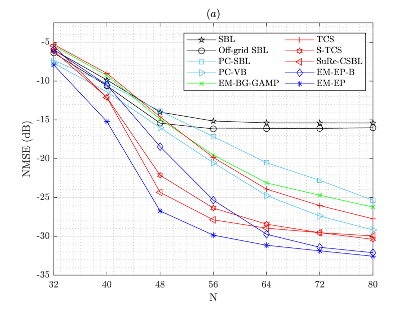
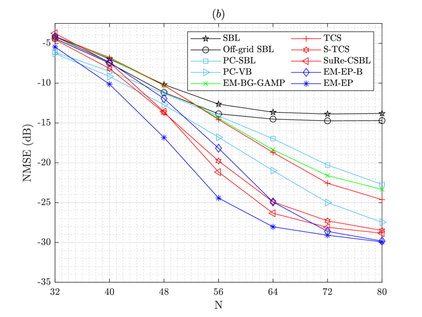
Figure 5: Channel estimation error vs. number of pilot symbols $N$ with parameters $G=128$, $M=200$, SNR=$10$ dB, and for $(a)$ $L_{s}=3$, $L_{p}=10$, and $A=10^{\text{o}}$, $(b)$ $L_{s}=4$, $L_{p}=10$, and $A=10^{\text{o}}$.

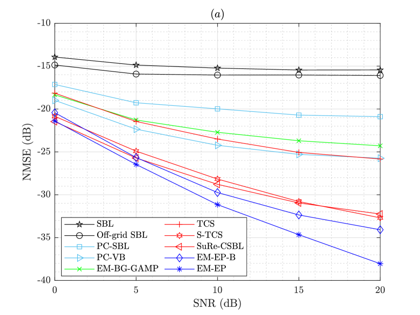
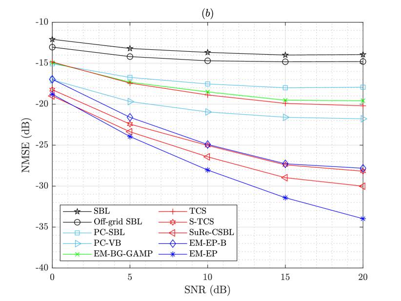
Figure 6: Channel estimation error vs. SNR (dB) with parameters $G=128$, $M=200$, $N=64$, and for $(a)$ $L_{s}=3$, $L_{p}=10$, and $A=10^{\text{o}}$, $(b)$ $L_{s}=4$, $L_{p}=10$, and $A=10^{\text{o}}$.

In order to compare our algorithm with the EP algorithm proposed in [33], we need to extend this algorithm. In [33] the authors modeled the elements of the support (latent) vector $\mathbf{z}$ with an iid Bernoulli prior distribution having a parameter $p_{0}$ which, along with the other model parameters, is assumed to be known. To apply their approach to the problem under consideration here, we need to estimate these parameters. Therefore we extend the method in [33] with the EM algorithm as discussed in section II and refer to the resulting algorithm as EM-EP-B. More specifically, in the (l+1)-st iteration of EM-EP-B algorithm, $p_{0}$ is updated according to $p^{(l+1)}_{0}=\frac{1}{M}\sum^{M}_{m=1}\sigma(p^{(l+1)}_{m})$. Moreover, the other model parameters, i.e., $\eta$, $\gamma_{m}$, and (to integrate grid refining) $\bm{\theta}$ are updated using our results in (73), (74), and (76) from section IV.

We also show the performances of SBL [46], Off-grid SBL [17], PC-SBL [21], PC-VB [20], EM-BG-GAMP [24], TCS [23], S-TCS [10], and SuRe-CSBL [25]. For Off-grid SBL, PC-SBL, PC-VB, SuRe-CSBL, EM-EP-B, and EM-EP algorithms, the dictionary $\mathbf{A}(\bm{\theta})$ is initialized to be a (partial) DFT matrix. For the other algorithms, however, $\mathbf{A}(\bm{\theta})$ is the fixed DFT matrix as required for the derivation of the algorithms and state evolution analysis. In all the experiments, we initialized the EM-EP algorithm with $\lambda^{(0)}=0.3$, $\tau_{01}^{(0)}=0.1$, $\tau_{10}^{(0)}=\frac{\lambda^{(0)}}{1-\lambda^{(0)}}\tau^{(0)}_{01}$, $\eta^{(0)}=\gamma^{(0)}_{m}=\left(\frac{||\mathbf{y}||^{2}}{(SNR^{(0)}+1)N}\right)^{-1}$ with $SNR^{(0)}=100$, and $\theta^{(0)}_{m}=\text{sin}^{-1}\left(-1+\frac{2m}{M}\right)$ for $m=1,2,\ldots,M$ as in [24, 25]. The maximum iterations of EM and EP algorithms are set as $n_{EP}=n_{EM}=100$ and the tolerance coefficients are selected to be $\epsilon_{EP}=\epsilon_{EM}=10^{-4}$. The channel estimation error is computed by using the following normalized mean-squared-error (NMSE),

$$\text{NMSE (dB)}=10\log_{10}\frac{\mathbb{E}[||\hat{\mathbf{h}}-\mathbf{h}||^{2}]}{\mathbb{E}[||\mathbf{h}||^{2}]},$$ (78)

in which $\hat{\mathbf{h}}$ is the channel estimate.

In Fig. 4 we investigate the performance of the selected channel estimation algorithms for recovering the sparse vector $\mathbf{w}$ with non-uniform burst sparsityfoot_1. We consider a BS with $G=128$ antennas transmitting $N=48$ pilot symbols to the user with $SNR=10$ dB. The physical channel between the BS and the user has $L_{s}=3$ scatterers with $L_{p}=10$ paths per scatterer. The channel estimators assume a fixed uniformly-spaced angular grid with $\theta_{m}=\text{sin}^{-1}\left(-1+\frac{2m}{M}\right)$ for $m=1,2,\ldots,M$ with $M=200$, and the physical AoDs corresponding to the three non-zeros clusters are assumed to be located on the grid points at $m=81,82,\ldots,90$,$100,101,\ldots,109$, $122,123,124,128,129,\ldots,134$. We get the following observations from Fig. 4. Firstly, when the non-zero clusters are closely located as shown by the dotted lines in Fig. 4, the algorithms such as PC-VB which tune each coefficient based on the nearest neighbor, exhibit a performance loss due to the leakage of energy into the bins between the adjacent clusters. For instance, observe the energy leakage around $-3^{\text{o}}$, $8^{\text{o}}$, and $15^{\text{o}}$ in Fig. 4 (e). Secondly, the algorithms such as EM-EP-B and EM-BG-GAMP which aim to recover the coefficients individually result in outliers at random positions far away from the true AoDs. This effect, when pronounced as in the case of EM-BG-GAMP, causes significant performance loss. Thirdly, SuRe-CSBL and S-TCS which employ a Markov prior on the support vector $\mathbf{z}$ eliminate the outliers, but suffer from significant leakage of energy into the bins near the clusters true AoDs. Finally, our proposed EM-EP algorithm eliminates the leakage of energy as well as the occurrence of outliers, and much more accurately represents the channel.

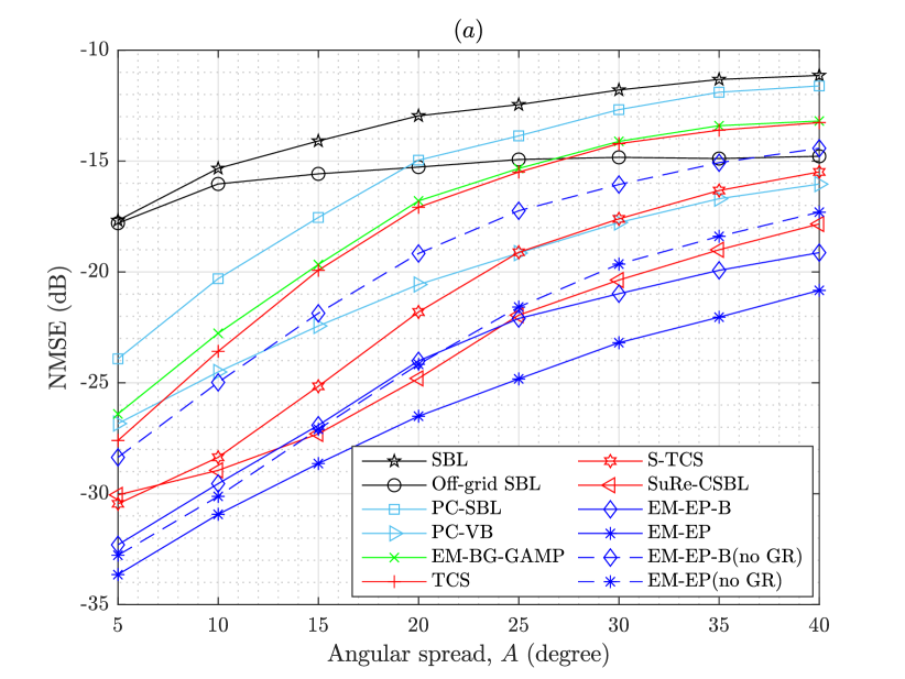
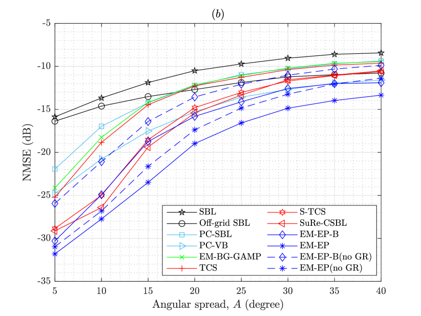
Figure 7: Channel estimation error vs. Angular spread $A$ with parameters $G=128$, $M=200$, $N=64$, and for $(a)$ $L_{s}=3$, $L_{p}=10$, and $SNR=10$ dB, $(b)$ $L_{s}=4$, $L_{p}=10$, and $SNR=10$ dB.

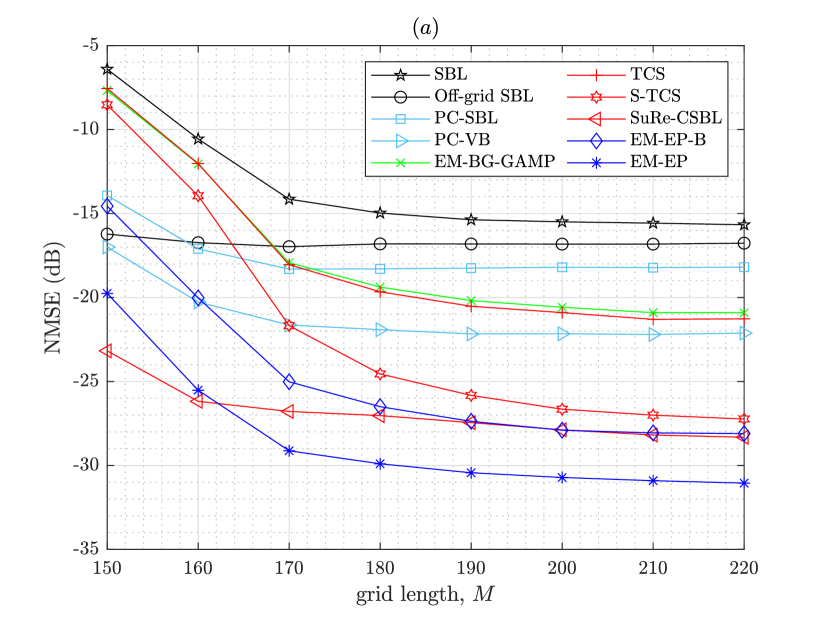
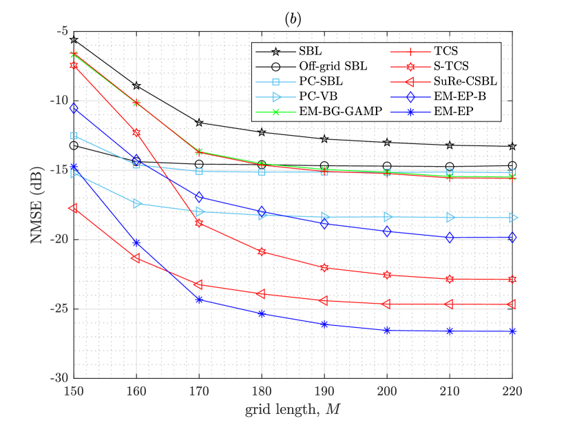
Figure 8: Channel estimation error vs. grid length $M$ with parameters $G=150$, $N=64$, $SNR=10$ dB, and for $(a)$ $L_{s}=3$, $L_{p}=10$, and $A=10^{\text{o}}$, $(b)$ $L_{s}=4$, $L_{p}=10$, and $A=10^{\text{o}}$.

Fig. 5 shows the channel estimation error versus the number of pilot symbols $N$ for the selected channel estimation schemes. We consider the massive MIMO channel with $L_{s}=3$ or $4$ scatterers and $L_{p}=10$ paths per scatterer. The AoDs for all the paths are randomly generated continuous-valued parameters with no on-grid assumption as before, and all the paths per scatterer are concentrated in an angular spread $A=10^{\text{o}}$. We observe that in both cases shown in Figs. 5(a) and 5(b), the performance of the algorithms improve with $N$ and EM-EP significantly outperforms all the algorithms. The channel has more paths in case of $L_{s}=4$ in Fig. 5(b) and thus larger values of $N$ are required to reach the same level of performance. SBL, Off-grid SBL, EM-BG-GAMP, and EM-EP-B aim to recover the coefficients individually and hence their performance is degraded due to the occurrence of outliers in the angular domain. Compared to SBL and Off-grid SBL which assume an iid complex Gaussian prior on $\mathbf{w}$, EM-BG-GAMP, TCS, and EM-EP-B assume an iid Bernoulli-Gaussian (BG) prior where the level of sparsity in $\mathbf{w}$ is directly adjusted by the weight of the Bernoulli component. This weight determines the fraction of coefficients that are a priori set to zero. Thus, EM-BG-GAMP and TCS perform better than the SBL-based algorithms. On the other hand, EM-EP-B includes the correlations in $\mathbf{w}$ by using $\bm{\Sigma}$ in its estimation of the posterior distribution and also performs grid refining to learn the dictionary. Therefore EM-EP-B outperforms both EM-BG-GAMP and TCS. PC-SBL and PC-VB aim to recover each coefficient in $\mathbf{w}$ according to its nearest neighbor. PC-SBL uses an SBL-based algorithm and tunes the precision of each coefficient according to the precisions of its immediate neighbors but using a sub-optimal solution. PC-VB avoids this sub-optimality by linking a support vector with a multinoulli prior to every coefficient and using a variational Bayes (VB) [22] based algorithm. Hence, PC-VB performs better than PC-SBL, but its performance suffers due to the leakage of energy when multiple non-zeros clusters are closely located. Performance of PC-VB is inferior to that of EM-EP-B. Due to its dependence on the VB method, PC-VB may approximate the true distribution locally around one of its several sub-optimal modes, whereas EM-EP-B employs the EP method which approximates the true distribution globally over a wider support and thus results in a better performance [36]. Finally in contrast to S-TCS and SuRe-CSBL, EM-EP takes into account the correlation in $\mathbf{w}$ thereby outperforming the former two algorithms.

Fig. 6 shows the channel estimation error versus SNR for the selected algorithms. We consider the same scenario as in Fig. 5 except that the number of pilot symbols is now fixed to $N=64$. We observe that the performance of the algorithms improves with SNR and the proposed EM-EP algorithm has the best performance of all the schemes. In case of $L_{s}=4$ scatterers the channel has more paths and therefore has more chances of having non-equal size clusters. Therefore in this case the performance of EM-EP-B which aims to recover the coefficients individually deteriorates and is worse than that of SuRe-CSBL. Fig. 6 also shows that while the performance of all the methods reaches a floor at some value of SNR (This is more evident in Fig. 6(b).), the proposed EM-EP continues to improve with SNR.

Fig. 7 shows the channel estimation error for different values of the angular spread $A$. We consider two cases of $L_{s}=3$ and $L_{s}=4$ scatterers as before and with $G=128$, $M=200$, and $N=64$. The SNR value is fixed to $10$ dB. As $A$ increases severe non-equal size burst sparsity may exist with isolated paths, and thus as observed from Fig. 7 the performance of the algorithms degrades accordingly. For a fixed $A$, such non-equal size burst sparsity becomes more intense when the channel has more paths as in case (b), and hence the channel estimation errors are relatively higher. However, in both cases the EP-based algorithms show significant gains in performance, and the proposed EM-EP algorithm outperforms all the algorithms. In Fig. 7 we also show the performance of EM-EP when no grid refining is performed, i.e., no optimization over AoDs $\bm{\theta}$, denoted in Fig. 7 as EM-EP(no-GR). It can be seen that EM-EP(no-GR) performs better than most of the other algorithms due to the use of the EP method and taking into account the correlation in $\mathbf{w}$.

In Fig. 8 we examine the effect of varying the grid length $M$ on the channel estimation performance of the algorithms. Consider the channel with $L_{s}=3$ or $4$ scatterer where the BS has $G=150$ antennas, the number of pilot symbols are fixed to $N=64$, angular spread is selected to be $A=10^{\text{o}}$, and the SNR is set to $10$ dB. It is observed that in both cases shown in Fig. 8 the performance of the algorithms improve with $M$, and our proposed EM-EP algorithm outperforms all the algorithms for large $M$. The parameter $M$ defines the resolution of the initial angular grid which is here given by $\Delta\theta^{(0)}=\text{sin}^{-1}(2/M)$. When $M$ is small, the initial grid is coarse and thus the algorithms suffer from convergence to local minima resulting in higher channel estimation error. As $M$ increases the grid resolution improves which in turn improves the channel estimation performance of the algorithms. Further, for a fixed number of paths, as $M$ increases the level of sparsity increases and thus the non-zero coefficients are more successfully recovered by the algorithms.

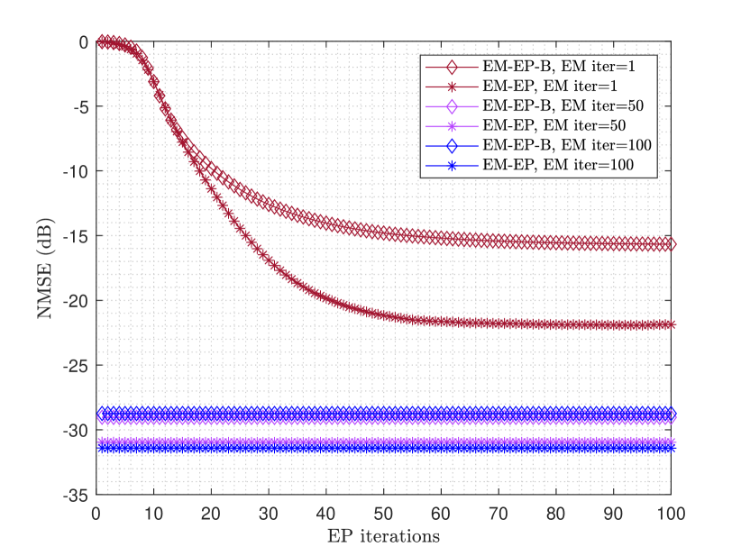
Figure 9: Channel estimation error vs. EP iterations when EM iterations are either 1, 50, or 100, and other parameters are $G=128$, $N=64$, $M=200$, $L_{s}=3$, $L_{p}=10$, and $A=10^{\text{o}}$.

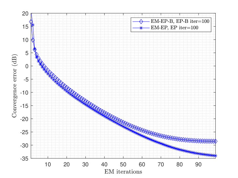
Figure 10: Convergence error of estimating the model parameters $\bm{\xi}$ vs. EM iterations when EP-B and EP iterations are 100, and other parameters are $G=128$, $N=64$, $M=200$, $L_{s}=3$, $L_{p}=10$, and $A=10^{\text{o}}$.

Fig. 10 shows the average channel estimation performance of the EM-EP-B and EM-EP algorithms over the EP iterations when the EM iterations for both algorithms are either fixed to 1, 50, or 100. The normalized mean squared error plotted in the figure is computed after the selected number of EM iterations are run, and thus the error corresponds to the EP run in the last iteration of EM. The estimation error is defined as $\text{NMSE (dB)}=10\log_{10}\frac{\mathbb{E}\left[||\mathbf{h}_{n}-\mathbf{h}||^{2}\right]}{\mathbb{E}\left[||\mathbf{h}||^{2}\right]}$ where $\mathbf{h}_{n}$ is the channel estimate obtained at the $n$-th iteration of the EP-B or EP algorithm. We see that when the EM iteration is fixed to 1, our proposed EP algorithm converges faster than the EP-B algorithm with a significant improvement in channel estimation. As the EM iterations increase both algorithms converge in just 3 iterations, but as expected EM-EP continues to maintain a small edge in channel estimation performance. This improvement in the convergence performance of the EP-based algorithms is achieved due to the following two reasons. Each full run of the EP-B and EP algorithms in an EM iteration is initialized using the approximate distribution $Q(\mathbf{w},\mathbf{z})$ obtained in the previous EM iteration. Our experiments show that such initialization of the EP algorithm results in an improved estimation and convergence performances. Another reason is that as the EM iterations continue, the EM estimates of the model parameters $\bm{\xi}$ converges to the local maximum of the likelihood function $p(\mathbf{y}|\bm{\xi})$, and the EP-based algorithms closely approximate the true joint posterior distribution on the sparse vector and its support.

Finally, in Fig. 10 we show the average convergence error performance of the EM-EP-B and EM-EP algorithms in estimating the model parameters $\bm{\xi}$ over the EM iterations. The iterations of the EP-B and EP algorithms are fixed to 100 and the results are averaged over $1000$ Monte Carlo trials. The convergence error plotted in the figure is defined as $\text{convergence error (dB)}=10\log_{10}\frac{||\bm{\xi}^{(l+1)}-\bm{\xi}^{l}||^{2}}{||\bm{\xi}^{l}||^{2}}$ where index $l$ represents the $l$-th iteration of EM, and $l=1,2,\ldots,n_{EM}$. It is observed that in the first four iterations the error of EM-EP is larger than EM-EP-B due to the fact that EM-EP is also estimating the Markov transition probabilities $\tau_{01}$ and $\tau_{10}$. However, after that EM-EP outperforms EM-EP-B. Moreover, after 70-80 iterations EM-EP-B has reached a plateau whereas EM-EP continues to improve. As observed the convergence error reduces with the EM iterations until the EM estimates converges to a local maximum of the objective function. Furthermore, comparing Figs. 10 and 10, we observe that after 50 EM iterations, any further EM iteration does not improve the channel estimation performance of EM-EP-B algorithm, whereas as expected our proposed EM-EP algorithm continues to improve.

VI Conclusions

We consider the problem of downlink channel estimation in the multi-user massive MIMO systems. To capture the clustered sparse nature of the channel, we assume a conditionally independent identically distributed Bernoulli-Gaussian prior on the sparse vector representing the channel, and a Markov prior on its support vector. We develop an expectation propagation (EP) based algorithm to approximate the intractable joint distribution on the sparse vector and its support with a distribution from an exponential family. To find the maximum likelihood estimates of the hyperparameters and the angular grid points, we integrated the EP algorithm with the expectation maximization (EM) algorithm. The resulting EM-EP algorithm directly estimates the hyperparameters and the clustered sparse downlink channel. Simulation results show that due to the inclusion of the correlations in the sparse vector in the approximated posterior and the use of EP method, our EM-EP algorithm can recover the channel with non-equal size burst sparsity. Further, the proposed EM-EP algorithm outperforms the existing algorithms in the literature including S-TCS and SuRe-CSBL algorithms which also use a Markov prior on the support vector.

Appendix A: Proof of Lemma 1

Given the hybrid posterior distribution as

$$R_{2,m}(w_{m},z_{m}) =\frac{1}{C_{m}}p(w_{m}|z_{m})\mathcal{CN}(w_{m};\mu_{\backslash 2,m},\Sigma_{\backslash 2,m})\times$$

$$\quad\text{Bern}(z_{m};\sigma(p_{\backslash 2,m})),$$ (79)

where the normalization constant $C_{m}$ is written as

$$C_{m} =\sum_{z_{m}\in\{0,1\}}\int p(w_{m}|z_{m})\mathcal{CN}(w_{m};\mu_{\backslash 2,m},\Sigma_{\backslash 2,m})\times$$

$$\quad\text{Bern}(z_{m};\sigma(p_{\backslash 2,m}))dw_{m},$$ (80)

First, we compute $\frac{\partial\ln C_{m}}{\partial\mu^{*}_{\backslash 2,m}}$ in (82) which can be written as

$$\frac{\partial\ln C_{m}}{\partial\mu^{*}_{\backslash 2,m}} =\frac{\mathbb{E}_{R_{2,m}}[w_{m}]}{\Sigma_{\backslash 2,m}}-\frac{\mu_{\backslash 2,m}}{\Sigma_{\backslash 2,m}},$$ (81)

$$\partial\ln C_{m}=\frac{1}{C_{m}}\sum_{z_{m}\in\{0,1\}}\int p(w_{m}|z_{m})\partial\left[\mathcal{CN}(w_{m};\mu_{\backslash 2,m},\Sigma_{\backslash 2,m})\right]\text{Bern}(z_{m};\sigma(p_{\backslash 2,m}))dw_{m},$$

$$=\frac{1}{C_{m}}\sum_{z_{m}\in\{0,1\}}\int p(w_{m}|z_{m})\mathcal{CN}(w_{m};\mu_{\backslash 2,m},\Sigma_{\backslash 2,m})\text{Bern}(z_{m};\sigma(p_{\backslash 2,m}))\left[\frac{w_{m}-\mu_{\backslash 2,m}}{\Sigma_{\backslash 2,m}}\right]dw_{m}\partial\mu^{*}_{\backslash 2,m},$$ (82)

$$\partial\ln C_{m}=\frac{1}{C_{m}}\sum_{z_{m}\in\{0,1\}}\int p(w_{m}|z_{m})\partial\left[\mathcal{CN}(w_{m};\mu_{\backslash 2,m},\Sigma_{\backslash 2,m})\right]\text{Bern}(z_{m};\sigma(p_{\backslash 2,m}))dw_{m}$$

$$=\frac{1}{C_{m}}\sum_{z_{m}\in\{0,1\}}\int p(w_{m}|z_{m})\mathcal{CN}(w_{m};\mu_{\backslash 2,m},\Sigma_{\backslash 2,m})\text{Bern}(z_{m};\sigma(p_{\backslash 2,m}))$$

$$~{}~{}~{}~{}~{}~{}~{}~{}~{}~{}~{}~{}~{}~{}~{}~{}~{}~{}~{}\times\Big{[}\frac{|w_{m}-\mu_{\backslash 2,m}|^{2}}{\left(\Sigma_{\backslash 2,m}\right)^{2}}-\frac{1}{\Sigma_{\backslash 2,m}}\Big{]}dw_{m}\partial\Sigma_{\backslash 2,m},$$ (83)

$$\partial\ln C_{m}=\frac{1}{C_{m}}\sum_{z_{m}\in\{0,1\}}\int p(w_{m}|z_{m})\mathcal{CN}(w_{m};\mu_{\backslash 2,m},\Sigma_{\backslash 2,m})\partial\left[\text{Bern}(z_{m};\sigma(p_{\backslash 2,m}))\right]d_{w_{m}}$$

$$=\frac{1}{C_{m}}\sum_{z_{m}\in\{0,1\}}\int p(w_{m}|z_{m})\mathcal{CN}(w_{m};\mu_{\backslash 2,m},\Sigma_{\backslash 2,m})\text{Bern}(z_{m};\sigma(p_{\backslash 2,m}))$$

$$~{}~{}~{}~{}~{}~{}~{}~{}~{}~{}~{}~{}~{}~{}~{}~{}~{}~{}~{}\times\Big{[}\frac{z_{m}}{\sigma(p_{\backslash 2,m})}-\frac{(1-z_{m})}{(1-\sigma(p_{\backslash 2,m}))}\Big{]}d{w_{m}}\partial\sigma(p_{\backslash 2,m}),$$ (84)

$$S_{3,m-1,m}(z_{m-1},z_{m})$$

$$\propto\text{exp}\Big{\{}z_{m-1}\ln\frac{\sigma\left(p^{\backslash R}_{3,m-1}\right)\tau_{10}}{\sigma\left(-p^{\backslash R}_{3,m-1}\right)(1-\tau_{01})}+z_{m}\ln\frac{\sigma\left(p^{\backslash F}_{3,m}\right)\tau_{01}}{\sigma\left(-p^{\backslash F}_{3,m}\right)(1-\tau_{01})}$$

$$~{}~{}~{}~{}~{}~{}~{}~{}~{}~{}~{}~{}~{}~{}~{}~{}~{}~{}~{}~{}~{}~{}~{}+z_{m-1}z_{m}\ln\frac{(1-\tau_{10})(1-\tau_{01})}{\tau_{10}\tau_{01}}\Big{\}},$$ (85)

Setting $\mu_{m}=\mathbb{E}_{R_{2,m}}[w_{m}]$ in (81) and rearranging it we get

$$\mu_{m}=\mu_{\backslash 2,m}+\Sigma_{\backslash 2,m}\frac{\partial\ln C_{m}}{\partial\mu^{*}_{\backslash 2,m}},$$ (86)

Next we compute $\frac{\partial\ln C_{m}}{\partial\Sigma_{\backslash 2,m}}$ in (83) and write it as

$$\frac{\partial\ln C_{m}}{\partial\Sigma_{\backslash 2,m}} =\frac{\mathbb{E}_{R_{2,m}}\left[\mid w_{m}-\mu_{\backslash 2,m}\mid^{2}\right]}{\left(\Sigma_{\backslash 2,m}\right)^{2}}-\frac{1}{\Sigma_{\backslash 2,m}},$$ (87)

Expanding the $\mathbb{E}_{R_{2,m}}[.]$ operator in (87) and using (86) in it then rearranging gives

$$\mathbb{E}_{R_{2,m}}[|w_{m}|^{2}]=\Sigma_{\backslash 2,m}+\left(\Sigma_{\backslash 2,m}\right)^{2}\frac{\partial\ln C_{m}}{\partial\Sigma_{\backslash 2,m}}+|\mu_{\backslash 2,m}|^{2}+$$

$$\Sigma_{\backslash 2,m}\mu_{\backslash 2,m}\frac{\partial\ln C_{m}}{\partial\mu_{\backslash 2,m}}+\Sigma_{\backslash 2,m}\mu^{*}_{\backslash 2,m}\frac{\partial\ln C_{m}}{\partial\mu^{*}_{\backslash 2,m}},$$ (88)

subtracting $|\mathbb{E}_{R_{2,m}}[w_{m}]|^{2}$ from both sides of (88) and using (38) and (86) we get

$$\Sigma_{m,m}=\Sigma_{\backslash 2,m}+\left(\Sigma_{\backslash 2,m}\right)^{2}\left[\frac{\partial\ln C_{m}}{\partial\Sigma_{\backslash 2,m}}-\frac{\partial\ln C_{m}}{\partial\mu^{*}_{\backslash 2,m}}\frac{\partial\ln C_{m}}{\partial\mu_{\backslash 2,m}}\right],$$ (89)

Finally we compute $\frac{\partial\ln C_{m}}{\partial\sigma(p_{\backslash 2,m})}$ in (84) which can be written as

$$\frac{\partial\ln C_{m}}{\partial\sigma(p_{\backslash 2,m})}=\frac{\mathbb{E}_{R_{2,m}}[z_{m}]}{\sigma(p_{\backslash 2,m})}-\frac{(1-\mathbb{E}_{R_{2,m}}[z_{m}])}{(1-\sigma(p_{\backslash 2,m}))},$$ (90)

rearranging (90) and using (39) we get

$$\sigma(p_{m})=\sigma(p_{\backslash 2,m})+\sigma(p_{\backslash 2,m})(1-\sigma(p_{\backslash 2,m}))\frac{\partial\ln C_{m}}{\partial\sigma(p_{\backslash 2,m})},$$ (91)

where using (33), we compute

$$\frac{\partial\ln C_{m}}{\partial\sigma(p_{\backslash 2,m})} =\frac{1}{C_{m}}\left[\mathcal{CN}(0;\mu_{\backslash 2,m},\Sigma_{\backslash 2,m}+\gamma^{-1}_{m})-\right.$$

$$\quad\left.\mathcal{CN}(0;\mu_{\backslash 2,m},\Sigma_{\backslash 2,m})\right],$$ (92)

inserting (92) in (91) and again using (33) gives (40).

Appendix B: deriving the marginals in (57) and (58)

Let the joint probability mass function (pmf) on $z_{m-1}$ and $z_{m}$ can be defined as $p(z_{m-1}=i,z_{m}=j)=\phi_{ij}$ for $i,j\in\{00,01,10,11\}$. This pmf can be written as

$$p(z_{m-1},z_{m}) =\left[\phi_{11}\right]^{z_{m-1}z_{m}}\left[\phi_{01}\right]^{(1-z_{m-1})z_{m}}\times$$

$$\left[\phi_{10}\right]^{z_{m-1}(1-z_{m})}\left[\phi_{00}\right]^{(1-z_{m-1})(1-z_{m})},$$ (93)

$$\propto\text{exp}\{z_{m-1}\ell_{1}+z_{m}\ell_{2}+z_{m-1}z_{m}\ell_{3}\},$$ (94)

where we define

$$\ell_{1}=\ln\frac{\phi_{10}}{\phi_{00}},\quad\ell_{2}=\ln\frac{\phi_{01}}{\phi_{00}},\quad\ell_{3}=\ln\frac{\phi_{00}\phi_{11}}{\phi_{01}\phi_{10}},$$ (95)

Next we use (95) and $\sum_{i,j}\phi_{ij}=1$ to get the solution to this system of equations as

$$\phi_{00}=\frac{1}{1+\text{exp}\{\ell_{1}\}+\text{exp}\{\ell_{2}\}+\text{exp}\{\ell_{1}+\ell_{2}+\ell_{3}\}},$$ (96)

$$\phi_{01}=\frac{\text{exp}\{\ell_{2}\}}{1+\text{exp}\{\ell_{1}\}+\text{exp}\{\ell_{2}\}+\text{exp}\{\ell_{1}+\ell_{2}+\ell_{3}\}},$$ (97)

$$\phi_{10}=\frac{\text{exp}\{\ell_{1}\}}{1+\text{exp}\{\ell_{1}\}+\text{exp}\{\ell_{2}\}+\text{exp}\{\ell_{1}+\ell_{2}+\ell_{3}\}},$$ (98)

$$\phi_{11}=\frac{\text{exp}\{\ell_{1}+\ell_{2}+\ell_{3}\}}{1+\text{exp}\{\ell_{1}\}+\text{exp}\{\ell_{2}\}+\text{exp}\{\ell_{1}+\ell_{2}+\ell_{3}\}},$$ (99)

Now the joint distribution on $z_{m-1}$ and $z_{m}$ in our case is given in (56) as

$$S_{3,m-1,m}(z_{m-1},z_{m}) =q^{\backslash R}_{3,m-1}(z_{m-1})p(z_{m}|z_{m-1})q^{\backslash F}_{3,m}(z_{m}),$$ (100)

using (II), (51), and (54) in (100) and simplifying we get (85). Comparing (94) and (85), we see that

$$\ell_{1} =\ln\frac{\sigma\left(p^{\backslash R}_{3,m-1}\right)\tau_{10}}{\sigma\left(-p^{\backslash R}_{3,m-1}\right)(1-\tau_{01})},$$ (101)

$$\ell_{2} =\ln\frac{\sigma\left(p^{\backslash F}_{3,m}\right)\tau_{01}}{\sigma\left(-p^{\backslash F}_{3,m}\right)(1-\tau_{01})},$$ (102)

$$\ell_{3} =\ln\frac{(1-\tau_{10})(1-\tau_{01})}{\tau_{10}\tau_{01}},$$ (103)

and using the above equations in (96)-(99) we get

$$\phi_{00} =\frac{1}{D_{m}}\sigma(-p^{\backslash R}_{3,m-1})\sigma(-p^{\backslash F}_{3,m})(1-\tau_{01}),$$ (104)

$$\phi_{01} =\frac{1}{D_{m}}\sigma(-p^{\backslash R}_{3,m-1})\sigma(p^{\backslash F}_{3,m})\tau_{01},$$ (105)

$$\phi_{10} =\frac{1}{D_{m}}\sigma(p^{\backslash R}_{3,m-1})\sigma(-p^{\backslash F}_{3,m})\tau_{10},$$ (106)

$$\phi_{11} =\frac{1}{D_{m}}\sigma(p^{\backslash R}_{3,m-1})\sigma(p^{\backslash F}_{3,m})(1-\tau_{10}),$$ (107)

where the normalization constant $D_{m}$ is given by

$$D_{m}$$

$$=\sigma(-p^{\backslash R}_{3,m-1})\sigma(-p^{\backslash F}_{3,m})(1-\tau_{01})+\sigma(p^{\backslash R}_{3,m-1})\sigma(-p^{\backslash F}_{3,m})\tau_{10}$$

$$+\sigma(-p^{\backslash R}_{3,m-1})\sigma(p^{\backslash F}_{3,m})\tau_{01}+\sigma(p^{\backslash R}_{3,m-1})\sigma(p^{\backslash F}_{3,m})(1-\tau_{10}),$$ (108)

Now once $\phi_{ij}$s’ are computed in (104)-(107), the marginal distributions on $z_{m-1}$ and $z_{m}$ can be found from

$$S_{3,m-1}(z_{m-1}) =\left[\phi_{10}+\phi_{11}\right]^{z_{m-1}}\left[\phi_{01}+\phi_{00}\right]^{(1-z_{m-1})},$$ (109)

$$S_{3,m}(z_{m}) =\left[\phi_{01}+\phi_{11}\right]^{z_{m}}\left[\phi_{10}+\phi_{00}\right]^{(1-z_{m})},$$ (110)

where (109) and (110) is derived from (93) by marginalizing over the other variable. Notice that the means of these marginal distributions are given by $\mathbb{E}_{S_{3,m-1}}[z_{m-1}]=\phi_{10}+\phi_{11}$ and $\mathbb{E}_{S_{3,m}}[z_{m}]=\phi_{01}+\phi_{11}$ which can be easily computed using (104)-(107).

References

- [1] J. Shen, J. Zhang, E. Alsusa, and K. B. Letaief, “Compressed CSI Acquisition in FDD Massive MIMO: How Much Training is Needed?” IEEE Transactions on Wireless Communications, vol. 15, no. 6, pp. 4145–4156, June 2016.
- [2] S. Ji, Y. Xue, and L. Carin, “Bayesian Compressive Sensing,” IEEE Transactions on Signal Processing, vol. 56, no. 6, pp. 2346–2356, June 2008.
- [3] E. J. Candes and M. B. Wakin, “An Introduction To Compressive Sampling,” IEEE Signal Processing Magazine, vol. 25, no. 2, pp. 21–30, March 2008.
- [4] R. Zhang, H. Zhao, and J. Zhang, “Distributed Compressed Sensing Aided Sparse Channel Estimation in FDD Massive MIMO System,” IEEE Access, vol. 6, pp. 18 383–18 397, 2018.
- [5] W. U. Bajwa, J. Haupt, A. M. Sayeed, and R. Nowak, “Compressed Channel Sensing: A New Approach to Estimating Sparse Multipath Channels,” Proceedings of the IEEE, vol. 98, no. 6, pp. 1058–1076, June 2010.
- [6] Y. Zhou, M. Herdin, and A. Sayeed, “Experimental Study of MIMO Channel Statistics and Capacity via Virtual Channel Representation,” University of Wisconsin-Madison, Madison, WI, USA, Tech. Rep., 2007.
- [7] S. K. Sahoo and A. Makur, “Signal Recovery from Random Measurements via Extended Orthogonal Matching Pursuit,” IEEE Transactions on Signal Processing, vol. 63, no. 10, pp. 2572–2581, May 2015.
- [8] M. F. Duarte and Y. C. Eldar, “Structured Compressed Sensing: From Theory to Applications,” IEEE Transactions on Signal Processing, vol. 59, no. 9, pp. 4053–4085, Sep. 2011.
- [9] X. Rao and V. K. N. Lau, “Distributed Compressive CSIT Estimation and Feedback for FDD Multi-User Massive MIMO Systems,” IEEE Transactions on Signal Processing, vol. 62, no. 12, pp. 3261–3271, June 2014.
- [10] L. Chen, A. Liu, and X. Yuan, “Structured Turbo Compressed Sensing for Massive MIMO Channel Estimation Using a Markov Prior,” IEEE Transactions on Vehicular Technology, vol. 67, no. 5, pp. 4635–4639, May 2018.
- [11] Z. Gao, L. Dai, Z. Wang, and S. Chen, “Spatially Common Sparsity Based Adaptive Channel Estimation and Feedback for FDD Massive MIMO,” IEEE Transactions on Signal Processing, vol. 63, no. 23, pp. 6169–6183, Dec 2015.
- [12] W. Wang, Y. Xiu, B. Li, and Z. Zhang, “FDD Downlink Channel Estimation Solution With Common Sparsity Learning Algorithm and Zero-Partition Enhanced GAMP Algorithm,” IEEE Access, vol. 6, pp. 11 123–11 145, 2018.
- [13] S. Srivastava, A. Mishra, A. Rajoriya, A. K. Jagannatham, and G. Ascheid, “Quasi-Static and Time-Selective Channel Estimation for Block-Sparse Millimeter Wave Hybrid MIMO Systems: Sparse Bayesian Learning (SBL) Based Approaches,” IEEE Transactions on Signal Processing, vol. 67, no. 5, pp. 1251–1266, March 2019.
- [14] M. E. Tipping, “Sparse Bayesian Learning and the Relevance Vector Machine,” J. Mach. Learn. Res., vol. 1, pp. 211–244, Sep. 2001.
- [15] Y. Ding and B. D. Rao, “Dictionary Learning-Based Sparse Channel Representation and Estimation for FDD Massive MIMO Systems,” IEEE Transactions on Wireless Communications, vol. 17, no. 8, pp. 5437–5451, Aug 2018.
- [16] Y. Ding and B. D. Rao, “Compressed Downlink Channel Estimation Based on Dictionary Learning in FDD Massive MIMO Systems,” in 2015 IEEE Global Communications Conference (GLOBECOM), Dec 2015, pp. 1–6.
- [17] J. Dai, A. Liu, and V. K. N. Lau, “FDD Massive MIMO Channel Estimation With Arbitrary 2D-Array Geometry,” IEEE Transactions on Signal Processing, vol. 66, no. 10, pp. 2584–2599, May 2018.
- [18] A. F. Molisch, A. Kuchar, J. Laurila, K. Hugl, and R. Schmalenberger, “Geometry-based directional model for mobile radio channels—principles and implementation,” European Transactions on Telecommunications, vol. 14, no. 4, pp. 351–359, 2003.
- [19] A. Liu, V. K. N. Lau, and W. Dai, “Exploiting Burst-Sparsity in Massive MIMO With Partial Channel Support Information,” IEEE Transactions on Wireless Communications, vol. 15, no. 11, pp. 7820–7830, Nov 2016.
- [20] J. Dai, A. Liu, and H. C. So, “Non-Uniform Burst-Sparsity Learning for Massive MIMO Channel Estimation,” IEEE Transactions on Signal Processing, vol. 67, no. 4, pp. 1075–1087, Feb 2019.
- [21] J. Fang, Y. Shen, H. Li, and P. Wang, “Pattern-Coupled Sparse Bayesian Learning for Recovery of Block-Sparse Signals,” IEEE Transactions on Signal Processing, vol. 63, no. 2, pp. 360–372, Jan 2015.
- [22] D. G. Tzikas, A. C. Likas, and N. P. Galatsanos, “The variational approximation for Bayesian inference,” IEEE Signal Processing Magazine, vol. 25, no. 6, pp. 131–146, November 2008.
- [23] J. Ma, X. Yuan, and L. Ping, “Turbo Compressed Sensing with Partial DFT Sensing Matrix,” IEEE Signal Processing Letters, vol. 22, no. 2, pp. 158–161, Feb 2015.
- [24] J. Vila and P. Schniter, “Expectation-maximization Bernoulli-Gaussian approximate message passing,” in 2011 Conference Record of the Forty Fifth Asilomar Conference on Signals, Systems and Computers (ASILOMAR), 2011, pp. 799–803.
- [25] Z. He, X. Yuan, and L. Chen, “Super-Resolution Channel Estimation for Massive MIMO via Clustered Sparse Bayesian Learning,” IEEE Transactions on Vehicular Technology, vol. 68, no. 6, pp. 6156–6160, June 2019.
- [26] M. Seeger, “Expectation propagation for exponential families,” University of California at Berkeley, 485 Soda Hall, Berkeley CA, USA, Tech. Rep., 2005.
- [27] Y. Qi and T. P. Minka, “Window-based expectation propagation for adaptive signal detection in flat-fading channels,” IEEE Transactions on Wireless Communications, vol. 6, no. 1, pp. 348–355, Jan 2007.
- [28] K. Ghavami and M. Naraghi-Pour, “MIMO detection with imperfect channel state information using expectation propagation,” IEEE Transactions on Vehicular Technology, vol. 66, no. 9, pp. 8129–8138, Sep. 2017.
- [29] K. Ghavami and M. Naraghi-Pour, “Noncoherent SIMO detection by expectation propagation,” in 2017 IEEE International Conference on Communications (ICC), May 2017, pp. 1–6.
- [30] ——, “Blind channel estimation and symbol detection for Multi-Cell Massive MIMO systems by expectation propagation,” IEEE Transactions on Wireless Communications, vol. 17, no. 2, pp. 943–954, Feb 2018.
- [31] M. Naraghi-Pour, M. Rashid, and C. Vargas-Rosales, “Semi-blind channel estimation and data detection for multi-cell massive mimo systems on time-varying channels,” 2020.
- [32] A. Braunstein, A. P. Muntoni, A. Pagnani, and M. Pieropan, “Compressed sensing reconstruction using Expectation Propagation,” Journal of Physics A: Mathematical and Theoretical, 2019.
- [33] J. M. Hernández-Lobato, D. Hernández-Lobato, and A. Suárez, “Expectation propagation in linear regression models with spike-and-slab priors,” Machine Learning, vol. 99, no. 3, pp. 437–487, Jun 2015.
- [34] D. Hernández-Lobato, J. M. Hernández-Lobato, and P. Dupont, “Generalized Spike-and-Slab Priors for Bayesian Group Feature Selection Using Expectation Propagation,” Journal of Machine Learning Research, vol. 14, pp. 1891–1945, 2013.
- [35] A. P. Dempster, N. M. Laird, and D. B. Rubin, “Maximum likelihood from incomplete data via the EM algorithm,” Journal of the Royal Statistical Society, Series B, vol. 39, no. 1, pp. 1–38, 1977.
- [36] C. M. Bishop, Pattern Recognition and Machine Learning (Information Science and Statistics). Berlin, Heidelberg: Springer-Verlag, 2006.
- [37] D. G. Tzikas, A. C. Likas, and N. P. Galatsanos, “The variational approximation for Bayesian inference,” IEEE Signal Processing Magazine, vol. 25, no. 6, pp. 131–146, November 2008.
- [38] K. P. Murphy, Machine Learning: A Probabilistic Perspective. The MIT Press, 2012.
- [39] T. P. Minka, “A Family of Algorithms for Approximate Bayesian Inference,” Ph.D. dissertation, Massachusetts Institute of Technology, Cambridge, MA, USA, 2001.
- [40] D. Tse and P. Viswanath, Fundamentals of Wireless Communication. New York, NY, USA: Cambridge University Press, 2005.
- [41] J. Shen, J. Zhang, E. Alsusa, and K. B. Letaief, “Compressed CSI Acquisition in FDD Massive MIMO: How Much Training is Needed?” IEEE Transactions on Wireless Communications, vol. 15, no. 6, pp. 4145–4156, June 2016.
- [42] Hyun-Chul Kim and Z. Ghahramani, “Bayesian Gaussian Process Classification with the EM-EP Algorithm,” IEEE Transactions on Pattern Analysis and Machine Intelligence, vol. 28, no. 12, pp. 1948–1959, Dec 2006.
- [43] R. M. Neal and G. E. Hinton, “A view of the EM algorithm that justifies incremental, sparse, and other variants,” in Learning in Graphical Models, M. I. Jordan, Ed. Dordrecht: Springer Netherlands, 1998.
- [44] J. Nocedal and S. J. Wright, Numerical Optimization, 2nd ed. New York, NY, USA: Springer, 2006.
- [45] 3GPP, “Universal mobile telecommunications system (UMTS); Spatial channel model for multiple input multiple output (MIMO) simulations,” 3GPP TR 25.996 version 11.0.0 Release 11, 2012.
- [46] D. P. Wipf and B. D. Rao, “Sparse Bayesian learning for basis selection,” IEEE Transactions on Signal Processing, vol. 52, no. 8, pp. 2153–2164, Aug 2004.