Discontinuous Petrov–Galerkin approximation of eigenvalue problems

Abstract.

In this paper, the discontinuous Petrov–Galerkin approximation of the Laplace eigenvalue problem is discussed. We consider in particular the primal and ultra weak formulations of the problem and prove the convergence together with a priori error estimates. Moreover, we propose two possible error estimators and perform the corresponding a posteriori error analysis. The theoretical results are confirmed numerically and it is shown that the error estimators can be used to design an optimally convergent adaptive scheme.

1. Introduction

DPG approximation of partial differential equations is a popular and effective technique which has reached a quite mature level of discussion within the scientific community. The literature about DPG is pretty rich. The method has been introduced in a series of papers [16, 18, 20, 29] during the last decade. Originally, the method has been presented as a technique to design an intrinsically stabilized scheme for advective problems. The main idea is to use a suitable discontinuous trial and test functions that are tailored for stability. The ideal DPG formulation is turned into a practical DPG formulation [23] where the test function space is easily computable and arbitrary close to the optimal one. The DPG formulation comes with a natural a posteriori error indicator that can be used for driving a robust $hp$ adaptivity. Moreover, it has been shown that for one dimensional problems the DPG method can be tuned to provide no phase errors in the case of time-harmonic wave propagation.

After these pioneer works, several studies have been performed, showing that the method can be applied to a variety of other problems. In particular: a solid analysis has been presented in the case of the Laplace equations [17]; the method has been proved locking free for linear elasticity [6]; it has been applied to Friedrichs-like systems [8], including convection-diffusion-reaction, linear continuum mechanics, time-domain acoustic, and a version of Maxwell’s equations; it has been applied to the Reissner–Mindlin plate bending model [9], to the Helmholtz equation [22], to the Stokes problem [25], to compressible flows [15], to the Navier–Stokes equations [26], and to the Maxwell equation [11].

In this paper, we are interested in the approximation of the Laplace eigenvalue problem. We study the so-called primal and ultra weak formulation of the Poisson problem: we refer the interested reader to [19, 17, 23] for the analysis and a discussion of the primal and ultra weak formulations for the Laplace problem in the case of the source problem. We will also look at a posteriori error estimators, perform an a posteriori analysis, and show numerically the optimal convergence of an adaptive scheme.

Following what was recently done for the Least-Squares finite element method [2, 3], we study how the DPG method can approximate eigenvalue problems.

After recalling the abstract setting for DPG approximations and the convergence of eigenvalues and eigenfunctions in Section 2, we apply the theoretical framework to the Laplace eigenvalue problem in Section 3, where we show the a priori estimates for the primal and ultra weak formulations. The a posteriori analysis is developed in Section 4 where we consider a natural error estimator related to what was studied in [10] and the alternative error estimator introduced in [24] which is based on a suitable characterization of the eigenfunctions in terms of Crouzeix–Raviart elements valid for the lowest order approximation. Finally, in Section 5 we present some numerical tests where the theory is confirmed and where it is shown that an adaptive scheme for the DPG approximation of the eigensolutions of the Laplace problem is optimally convergent.

2. Problem formulation and a priori analysis framework

We start by describing the general structure of a DPG source problem, since this is useful in order to introduce our notation before dealing with the corresponding eigenvalue problem.

The source problem we are studying is: find $u\in U$ such that

(1) $$b(u,v)=\ell(v)\quad\forall v\in V,$$

where $U$ is a trial Hilbert space and $V$ is a test Hilbert space. The bilinear form $b:U\times V\to\mathbb{C}$ satisfies the assumptions

(2) $$b(u,v)=0\quad\forall v\in V\Longrightarrow u=0$$

(3) $$0<C_{1}:=\inf_{u\in U\setminus\{0\}}\sup_{v\in V\setminus\{0\}}\frac{|b(w,v)|}{\|w\|_{U}\|v\|_{V}}\quad\forall v\in V$$

$\ell:V\to\mathbb{C}$ is a linear form.

The DPG formulation of (1) is obtained by introducing a discrete space $U_{h}\subset U$ and an optimal test function space given by $V_{opt}=T(U_{h})$, where $T:U\to V$ is the trial-to-test operator defined as: find $Tu\in V$ such that

(4) $$(Tu,v)_{V}=b(u,v)\quad\forall v\in V.$$

The discrete source problem is: find $u_{h}\in U_{h}$ such that

(5) $$b(u_{h},v)=\ell(v)\quad\forall v\in V_{opt}.$$

This is an ideal setting, since the actual computation of the test function space $V_{opt}$ is not feasible in most applications. In general a practical DPG method is adopted where the test space $V_{opt}$ is replaced by $V_{opt,h}$, obtained after introducing a finite dimensional subspace $V_{h}\subset V$ and defining a discrete trial-to-test operator $T_{h}$ as in (4) with $V$ replaced by $V_{h}$. Then the practical optimal test space is $V_{opt,h}=T_{h}(U_{h})$. If $V_{h}$ is a space of discontinuous piecewise polynomials, then the computation of the test functions is cheap, involving the solution of a block diagonal system.

We assume that there exists a linear operator $\Pi:V\to V_{h}$ and $C_{\Pi}$ such that for all $u_{h}\in U_{h}$ and all $v\in V$

(6) $$b(u_{h},v-\Pi v)=0$$

(7) $$\|\Pi v\|_{V}\leq C_{\Pi}\|v\|_{V}.$$

A fundamental characterization of the solution $u_{h}$ of the DPG system is given by the following mixed problem that is defined only via the discrete spaces $U_{h}$ and $V_{h}$ without the need of the trial-to-test operator $T$: find $u_{h}\in U_{h}$ and $\varepsilon_{h}\in V_{h}$ such that

(8) $$\left\{\begin{aligned} &(\varepsilon_{h},v_{h})_{V}+b(u_{h},v_{h})=\ell(v_{h})&&\forall v_{h}\in V_{h}\\ &\overline{b(z_{h},\varepsilon_{h})}=0&&\forall z_{h}\in U_{h}.\end{aligned}\right.$$

We are now ready to introduce the eigenvalue problem associated with (1) and its approximation corresponding to (8).

Usually the space $U$ consists of two components and can be presented as $U=U_{0}\times U_{1}$, where $U_{0}$ is a functional space defined on $\Omega$ (volumetric part) and $U_{1}$ is the remaining part that can be defined on $\Omega$ or on the skeleton of a given triangulation. Let $\mathcal{H}$ be a Hilbert pivot space so that we have the usual triplet $U_{0}\subset\mathcal{H}\simeq\mathcal{H}^{\prime}\subset U_{0}^{\prime}$ and consider a bilinear form $m:\mathcal{H}\times V\to\mathbb{C}$. The continuous eigenvalue problem is: find eigenvalues $\lambda\in\mathbb{C}$ and eigenfunctions $u=(u_{0},u_{1})\in U=U_{0}\times U_{1}$ with $u_{0}\neq 0$ such that

(9) $$b(u,v)=\lambda m(u_{0},v)\quad\forall v\in V.$$

In order to state the appropriate (compactness) assumptions, we introduce the solution operator $T_{F}:\mathcal{H}\to\mathcal{H}$ as follows: $T_{F}f\in\mathcal{H}$ is the component $u_{0}$ of the solution $u\in U$ to

(10) $$b(u,v)=m(f,v)\quad\forall v\in V.$$

We assume that (10) is uniquely solvable and the operator $T_{F}$ is compact.

The discrete space $U_{h}$ is analogously made of two components $U_{0,h}\subset U_{0}$ and $U_{1,h}\subset U_{1}$. The DPG discretization, corresponding to the mixed formulation (8), is given by: find $\lambda_{h}\in\mathbb{C}$ such that for some $u_{h}=(u_{0,h},u_{1,h})\in U_{h}=U_{0,h}\times U_{1,h}$ with $u_{0,h}\neq 0$ and some $\varepsilon_{h}\in V_{h}$ it holds

(11) $$\left\{\begin{aligned} &(\varepsilon_{h},v_{h})_{V}+b(u_{h},v_{h})=\lambda_{h}m(u_{0,h},v_{h})&&\forall v_{h}\in V_{h}\\ &\overline{b(z_{h},\varepsilon_{h})}=0&&\forall z_{h}\in U_{h}.\end{aligned}\right.$$

The matrix form of this formulation is given by

(12) $$\left(\begin{matrix}\mathsf{A}&\mathsf{B}^{\top}\\ \mathsf{B}&\mathsf{0}\end{matrix}\right)\left(\begin{matrix}\mathsf{x}\\ \mathsf{y}\end{matrix}\right)=\lambda\left(\begin{matrix}\mathsf{0}&\mathsf{M}\\ \mathsf{0}&\mathsf{0}\end{matrix}\right)\left(\begin{matrix}\mathsf{x}\\ \mathsf{y}\end{matrix}\right)$$

where $\mathsf{x}$ is the vector representation of $\varepsilon_{h}\in V_{h}$ and $\mathsf{y}$ of $u_{h}\in U_{h}$.

We introduce the discrete counterpart $T_{F,h}:\mathcal{H}\to\mathcal{H}$ of the solution operator $T_{F}$ as follows: $T_{F,h}f\in U_{0,h}\subset\mathcal{H}$ is the component $u_{0,h}\in U_{0,h}$ of the solution $u_{h}\in U$ of the following problem, for some $\varepsilon_{h}\in V_{h}$,

(13) $$\left\{\begin{aligned} &(\varepsilon_{h},v_{h})_{V}+b(u_{h},v_{h})=m(f,v_{h})&&\forall v_{h}\in V_{h}\\ &\overline{b(z_{h},\varepsilon_{h})}=0&&\forall z_{h}\in U_{h}.\end{aligned}\right.$$

In order show a priori estimates for the eigensolution computed with the DPG method we are going to use the classical Babǔska–Osborn theory [1, 4]. Let us denote by $\lambda_{i}$, $i=1,\dots$, the eigenvalues of the continuous problem (9) sorted such that

$$0<|\lambda_{1}|\leq|\lambda_{2}|\leq\cdots$$

and by $E_{i}=\mathrm{span}(u_{0,i})$, $i=1,\dots$, the corresponding eigenspaces. In case of multiple eigenvalues we repeat them so that each $E_{i}$ is one dimensional. Analogous notation $\lambda_{i,h}$ and $E_{i,h}$, $i=1,\dots$, is adopted for the discrete problem (11).

Theorem 1.

If the following convergence in norm holds true

(14) $$\|(T_{F}-T_{F,h})f\|_{\mathcal{H}}\leq\rho(h)\|f\|_{\mathcal{H}}\quad\forall f\in\mathcal{H}$$

with $\rho(h)$ tending to zero as $h$ goes to zero, then the discrete eigenvalues and eigenfunctions converge to the continuous ones. That is, any compact set $K$ included in the resolvent set of $T_{F}$ is included in the resolvent set of $T_{F,h}$ for $h$ small enough (absence of spurious modes); moreover, if $\lambda_{i}$ is an eigenvalue of algebraic multiplicity $m$ then there are exactly $m$ discrete eigenvalues $\lambda_{i_{j},h}$, $j=1,\dots m$, tending to $\lambda_{i}$ (convergence).

In order to estimate the rate of convergence, as usual, we shall make use of the gap between subspaces of Hilbert spaces defined as

$$\hat{\delta}(A,B)=\max\{\delta(A,B),\delta(B,A)\},$$

where

$$\delta(A,B)=\sup_{\begin{subarray}{c}a\in A\\ \|a\|=1\end{subarray}}\delta(a,B)$$

with

$$\delta(a,B)=\inf_{b\in B}\|a-b\|_{W}$$

for $A$ and $B$ closed subspaces of a Hilbert space $W$. If $W=U_{0}$ and $E$ is the $m$ dimensional eigenspace of the continuous problem corresponding to $\lambda_{i}$ (see the setting of Theorem 1), we introduce the following quantity related to $E$

$$\gamma_{h}=\|(T_{F}-T_{F,h})|_{E}\|_{\mathcal{L}(U_{0})}$$

and, if $E^{*}$ is the corresponding eigenspace of the adjoint operator $T_{F}^{*}$, we consider the following quantity

$$\gamma^{*}_{h}=\|(T_{F}^{*}-T_{F,h}^{*})|_{E^{*}}\|_{\mathcal{L}(U_{0}^{\prime})},$$

where $T_{F,h}^{*}$ is the discrete solution operator associated with the adjoint problem. Then we recall the following classical result.

Theorem 2.

Under the hypothesis of Theorem 1 it holds

$$\hat{\delta}(E_{h},E)\leq C\gamma_{h},$$

where $E_{h}$ is the direct sum of the eigenspaces of the $m$ eigenvalues approximating $\lambda_{i}$. Moreover, if $\alpha$ is the ascent multiplicity of $\lambda_{i}$, it holds

$$\max_{j=1,\dots,m}|\lambda_{i}-\lambda_{i_{j},h}|\leq C(\gamma_{h}\gamma_{h}^{*})^{1/\alpha}.$$

3. The Laplace eigenvalue problem

Let $\Omega\subset\mathbb{R}^{2}$ be a bounded polygonal domain. We are interested in the standard Dirichlet eigenvalue problem for the Poisson equation: find $\lambda$ such that for a nonzero $u$ we have

$$\left\{\begin{aligned} -\Delta u&=\lambda u&&\text{in }\Omega\\ u&=0&&\text{on }\partial\Omega.\end{aligned}\right.$$

We look at a conforming triangulation $\Omega_{h}$ and its skeleton $\partial\Omega_{h}$.

We will use two different formulations; namely, the so called primal and ultra-weak formulations (see, for instance, [19, 17, 23]).

3.1. Primal formulation

The formulation we are considering has been presented in [19] and fits within our setting with the following choices

$$U=U_{0}\times U_{1}$$

$$U_{0}=H^{1}_{0}(\Omega)$$

$$U_{1}=H^{-1/2}(\partial\Omega_{h})$$

$$\mathcal{H}=H^{1}(\Omega)$$

$$V=H^{1}(\Omega_{h})$$

$$b(u,\hat{\sigma}_{n};v)=(\operatorname{\nabla}u,\operatorname{\nabla}v)_{\Omega_{h}}-\langle\hat{\sigma}_{n},v\rangle_{\partial\Omega_{h}}$$

$$m(u,v)=(u,v)_{\Omega_{h}},$$

where as usual the symbol $\langle\cdot,\cdot\rangle_{\partial\Omega_{h}}$ denotes the action of a functional in $H^{-1/2}(\partial\Omega_{h})$ and $(\cdot,\cdot)_{\Omega_{h}}$ the broken $L^{2}$ scalar product. We recall the definition of $H^{-1/2}(\partial\Omega_{h})$ as

$$\left\{\tau\in\bigotimes_{K}H^{-1/2}(\partial K):\tau|_{\partial K}=\boldsymbol{\tau}\cdot\mathbf{n}|_{\partial K}\text{ for some }\boldsymbol{\tau}\in\mathbf{H}(\operatorname{\mathrm{div}};\Omega),\ \forall K\in\Omega_{h}\right\}.$$

We make use of the following discrete spaces for any integer $k\geq 1$

$$U_{h,0}=S^{k}_{0}(\Omega_{h})$$

$$U_{h,1}=P_{k-1}(\partial\Omega_{h})\cap U_{1}$$

$$U_{h}=U_{h,0}\times U_{h,1}$$

$$V_{h}=P_{k+1}(\Omega_{h}).$$

Here we denote

$$S^{k}_{0}(\Omega_{h}):=P_{k}(\Omega_{h})\cap C(\bar{\Omega}).$$

Remark 1.

In this section we are using the standard notation $u$ (resp. $u_{h}$) for the volumetric part of the solution and $\hat{\sigma}$ (resp. $\hat{\sigma}_{n}$) for the skeleton part. They correspond to $u_{0}$ (resp. $u_{0,h}$) and $u_{1}$ (resp. $u_{1,h}$) in the abstract presentation of the previous section. Analogous notation will be used in the next section for the ultra-weak formulation.

The uniform convergence (14) is usually proved by employing some a priori estimates of the source problem. The standard estimate for the source from [19] reads as follows

(15) $$\|u-u_{h}\|_{H^{1}(\Omega)}+\|\hat{\sigma}_{n}-\hat{\sigma}_{h,n}\|_{H^{-1/2}(\partial\Omega_{h})}$$

$$\qquad\leq C\inf_{(w_{h},\hat{r}_{h,n})\in U_{h}}(\|u-w_{h}\|_{H^{1}(\Omega)}+\|\hat{\sigma}_{n}-\hat{r}_{h,n}\|_{H^{-1/2}(\partial\Omega_{h})}).$$

Since we have chosen $\mathcal{H}=H^{1}(\Omega)$, the uniform convergence follows from (15) as it is shown in the next proposition.

Proposition 3.

Let $(u,\hat{\sigma}_{n})\in U$ be the solution of the source problem (1) with right hand side $f$ in $H^{1}(\Omega)$ and assume that $u$ belongs to $H^{1+s}(\Omega)$ for some $s\in(1/2,k+1]$, where $k$ is the order of the approximation introduced above. Then the uniform convergence (14) holds true.

Proof.

Let $(u_{h},\hat{\sigma}_{h})\in U_{h}$ be the numerical solution corresponding to our right hand side $f$ in $L^{2}(\Omega)$. Then the regularity assumptions together with the natural error estimates recalled above (see also [19, Eq. (5.1)] imply

$$\|u-u_{h}\|_{H^{1}(\Omega)}+\|\hat{\sigma}_{n}-\hat{\sigma}_{h,n}\|_{H^{-1/2}(\partial\Omega_{h})}\leq Ch^{s}\|f\|_{H^{1}(\Omega)}.$$

Due to the definitions $T_{F}(f)=u$ and $T_{F,h}(f)=u_{h}$ this implies

$$\|(T_{F}-T_{F,h})f\|_{H^{1}(\Omega)}\leq Ch^{s}\|f\|_{H^{1}(\Omega)},$$

which proves the uniform convergence (14) with $\mathcal{H}=H^{1}(\Omega)$ and $\rho(h)\leq Ch^{s}$. ∎

Corollary 4.

Proposition 3 holds also for the following discrete spaces for any odd integer $k\geq 1$

$$U_{h,0}=S^{k}_{0}(\Omega_{h})\ U_{h,1}=P_{k-1}(\partial\Omega_{h})\cap U_{1}$$

$$\tilde{V}_{h}=P_{k}(\Omega_{h}).$$

Proof.

The result follows from [5, Theorem 3.5] with the same arguments as in Proposition 3. ∎

We are now in a position to state our main conclusion of this section. For readiness, we consider the case of a simple eigenvalue. Natural modifications apply in case of higher multiplicity.

Theorem 5.

Let us consider the DPG primal approximation of the Laplace eigenvalue problem as discussed in Proposition 3. Then the conclusions of Theorems 1 and 2 hold true. In particular, let $\lambda$ be a simple eigenvalue of the continuous problem corresponding to an eigenspace $E$ belonging to $H^{1+s}(\Omega)$ and let $\lambda_{h}$ be the approximation of $\lambda$ with discrete eigenspace $E_{h}$. Then we have

(16) $$\hat{\delta}(E,E_{h})\leq Ch^{\tau}$$

$$|\lambda-\lambda_{h}|\leq Ch^{2\tau}$$

with $\tau:=\min\{s,k\}$.

Proof.

Theorem 1 follows from the convergence in norm (14) which we proved in Proposition 3.

In order to verify the rates of convergence shown in (16) we have to compute the quantities $\gamma_{h}$ and $\gamma^{*}_{h}$ related to the convergence of the DPG primal formulation and of its adjoint formulation, respectively. For the primal formulation, we can estimate $\gamma_{h}$ by using the optimal bound (15), thus obtaining

$$\gamma_{h}=O(h^{\tau})$$

which gives the first in (16).

The adjoint problem corresponding to the primal formulation has been considered extensively in [5] for the proof of a duality argument. In our notation, the continuous formulation of the adjoint problem corresponding to (8) (see [5, Eq. (20)]) is: given $g\in\mathcal{H}$, find $\varepsilon^{*}\in V$ and $\mathbf{u}^{*}=(u^{*},\hat{\sigma}_{n}^{*})\in U$ such that

(17) $$\left\{\begin{aligned} &(\varepsilon^{*},w)_{V}+(\operatorname{\nabla}u^{*},\operatorname{\nabla}w)_{\Omega_{h}}-\langle\hat{\sigma}_{n}^{*},w\rangle_{\partial\Omega_{h}}=0&&\forall w\in V\\ &(\operatorname{\nabla}\varepsilon^{*},\operatorname{\nabla}v)_{\Omega_{h}}=(g,v)_{\Omega_{h}}&&\forall v\in U_{0}\\ &\langle\hat{\tau}_{n},\varepsilon^{*}\rangle_{\partial\Omega_{h}}=0&&\forall\hat{\tau}_{n}\in U_{1}\end{aligned}\right.$$

In order to estimate $\gamma^{*}_{h}$ we need to consider the discretization of (17). It is apparent that the left hand side of the adjoint problem is the same as the one corresponding the standard primal formulation, so that, denoting by $(\varepsilon^{*}_{h},u^{*}_{h},\hat{\sigma}^{*}_{n,h})\in V_{h}\times U_{h,0}\times U_{h,1}$ the discrete solution, the following quasi-optimal a priori estimate holds true

(18) $$\|\varepsilon^{*}-\varepsilon^{*}_{h}\|_{V}+\|u^{*}-u^{*}_{h}\|_{U_{0}}+\|\hat{\sigma}_{n}^{*}-\hat{\sigma}^{*}_{n,h}\|_{U_{1}}$$

$$\qquad\leq\inf_{(\delta,v,\hat{\tau}_{n})\in V_{h}\times U_{h,0}\times U_{h,1}}(\|\varepsilon^{*}-\delta\|_{V}+\|u^{*}-v\|_{U_{0}}+\|\hat{\sigma}_{n}^{*}-\hat{\tau}_{n}\|_{U_{1}})$$

It remains to check the regularity of the solution of the dual problem (17). In [5, Eq. (21)] it is observed that the strong form of the dual problem is as follows

$$-\Delta\varepsilon^{*}=g \text{in }\Omega$$

$$\varepsilon^{*}=0 \text{on }\partial\Omega$$

$$\Delta u^{*}=\varepsilon^{*}+g \text{in }\Omega$$

$$u^{*}=0 \text{on }\partial\Omega$$

$$\hat{\sigma}_{n}^{*}=\operatorname{\nabla}(\varepsilon^{*}+u^{*})\cdot\mathbf{n} \text{on }\partial K\ \forall K\in\Omega_{h}$$

In particular, since the dual problem involves the Laplace operator, the regularity of its solution will be related to the same Sobolev exponent $1+s$ as for the original Laplace problem. This implies that from the rate of convergence predicted by (18) we can obtain

$$\gamma^{*}_{h}=O(h^{\tau})$$

Hence, the double order of convergence for the eigenvalues is proved, which concludes our proof. ∎

Theorem 5 estimates the eigenfunction error in the energy norm of $U_{0}$. It is interesting to observe that the when the error is estimated in $L^{2}(\Omega)$ then higher order can be achieved. This is stated in the following proposition.

Proposition 6.

Under the same assumptions and notation of Theorem 5, the following estimate holds true

(19) $$\hat{\delta}_{0}(E,E_{h})\leq Ch^{\upsilon+\tau}$$

with $\upsilon=\min\{s,1\}$, where $\hat{\delta}_{0}$ denotes the gap in the $L^{2}(\Omega)$ norm.

Proof.

The result is a consequence of the analogous one valid for the source problem which has been proved in [5, Thm. 3.1] in the case of a convex domain. This is a standard Aubin–Nitche duality argument. The general case follows by inspecting the proof of Theorem 3.1 dealing with Assumption 2.9 where the regularity of the dual (adjoint) problem is discussed. Reference [5] studies the case of full regularity $s=1$; when $s<1$ exactly the same arguments give the result with $C_{3}(h)=h^{s}$. ∎

We now switch back momentarily to the notation of the abstract setting, where the component $u$ of the solution was denoted by $u_{0}$ and the component $\hat{\sigma}$ by $u_{1}$. Then we observe that the convergence estimates in the first of (16) and in (19) imply that given $u_{0}\in E$ there exists $u_{0,h}\in E_{h}$ such that

(20) $$\|u_{0}-u_{0,h}\|_{U_{0}}\leq Ch^{\tau}\|u_{0}\|_{H^{1+s}(\Omega)}$$

$$\|u_{0}-u_{0,h}\|_{L^{2}(\Omega)}\leq Ch^{\tau+\upsilon}\|u_{0}\|_{H^{1+s}(\Omega)}.$$

When also the other component of the eigenfunction is considered, we have the following a priori estimate

(21) $$\|u-u_{h}\|_{U}\leq Ch^{\tau}\|u_{0}\|_{H^{1+s}(\Omega)}$$

where the components $u_{1}$ and $u_{1,h}$ of $u$ and $u_{h}$ are the ones corresponding to $u_{0}$ and $u_{0,h}$ in (9) and (11), respectively.

3.2. Ultra weak formulation

The DPG ultra weak formulation for the Laplace eigenvalue problem fits within our abstract setting with the following choices (see [17, 23] for more details):

$$U=U_{0}\times U_{1}$$

$$U_{0}=L^{2}(\Omega)$$

$$U_{1}=L^{2}(\Omega)^{2}\times H^{1/2}_{0}(\partial\Omega_{h})\times H^{-1/2}(\partial\Omega_{h})$$

$$\mathcal{H}=U_{0}$$

$$V=H^{1}(\Omega_{h})\times\mathbf{H}(\operatorname{\mathrm{div}};\Omega_{h})$$

$$b(u,\boldsymbol{\sigma},\hat{u},\hat{\sigma}_{n};v,\boldsymbol{\tau})=(\boldsymbol{\sigma},\boldsymbol{\tau})_{\Omega_{h}}-(u,\operatorname{\mathrm{div}}\boldsymbol{\tau})_{\Omega_{h}}+\langle\hat{u},\boldsymbol{\tau}\cdot\mathbf{n}\rangle_{\partial\Omega_{h}}$$

$$\hskip 85.35826pt-(\boldsymbol{\sigma},\operatorname{\nabla}v)_{\Omega_{h}}+\langle v,\hat{\sigma}_{n}\rangle_{\partial\Omega_{h}}$$

$$m(u;v,\boldsymbol{\tau})=(u,v)_{\Omega_{h}},$$

where the space $H^{1/2}_{0}(\partial\Omega_{h})$ is defined as

$$\left\{\hat{w}\in\bigotimes_{K}H^{1/2}(\partial K):\hat{w}|_{\partial K}=w|_{\partial K}\text{ for some }w\in H^{1}_{0}(\Omega),\ \forall K\in\Omega_{h}\right\}$$

and $H^{1}(\Omega_{h})$ and $\mathbf{H}(\operatorname{\mathrm{div}};\Omega_{h})$ denote broken functional spaces on the mesh $\Omega_{h}$.

We choose the following discrete spaces with $k\geq 0$

(22a) $$U_{h} :=P_{k}(\Omega_{h})\times P_{k}(\Omega_{h};\mathbb{R}^{2})\times S^{k+1}_{0}(\partial\Omega_{h})\times P_{k}(\partial\Omega_{h})$$

(22b) $$V_{h} :=P_{k+2}(\Omega_{h})\times P_{k+2}(\Omega_{h};\mathbb{R}^{2})$$

where $S^{k+1}_{0}(\partial\Omega_{h})$ is defined as follows

$$S^{k+1}_{0}(\partial\Omega_{h}):=\gamma_{0}(S^{k+1}_{0}(\Omega_{h})\cap H^{1}_{0}(\Omega)).$$

Here $\gamma_{0}$ denotes the canonical trace operator from $H^{1}(\Omega)$ to $H^{1/2}(\partial\Omega_{h})$.

Also in this case we can use the a priori estimates in order to show the uniform convergence (14).

Proposition 7.

Let $T_{F}:\mathcal{H}\to\mathcal{H}$ be the solution operator associated with the continuous problem and $T_{F,h}$ its discrete counterpart as defined in (10) and (13), respectively. Assume that the solution $u$ of the Poisson problem with $f$ in $L^{2}(\Omega)$ belongs to $H^{1+s}(\Omega)$ for some $s\in(1/2,k+1]$, where $k$ is the order of approximation used in (22). Then the convergence in norm (14) holds true.

Proof.

The a priori error analysis presented, for instance, in [21, Cor. 6] reads

$$\|u-u_{h}\|_{U_{0}}\leq Ch^{s}\|f\|_{L^{2}(\Omega)}$$

which implies the uniform convergence (14). ∎

The rate of convergence that follows naturally from the a priori error estimate for the source problem is presented in the following theorem.

Theorem 8.

Let us consider the DPG ultraweak approximation of the Laplace eigenvalue problem as discussed in Proposition 7. Then the conclusions of Theorems 1 and 2 hold true. In particular, let $\lambda$ be a simple eigenvalue of the continuous problem corresponding to an eigenspace $E$ belonging to $H^{1+s}(\Omega)$ and let $\lambda_{h}$ be the approximation of $\lambda$ with discrete eigenspace $E_{h}$. Then we have

$$\hat{\delta}(E,E_{h})\leq Ch^{\tau}$$

$$|\lambda-\lambda_{h}|\leq Ch^{2\tau}$$

with $\tau=\min\{s,k+1\}$.

Proof.

We omit the technical detail of the proof that follows the same lines as the proof of Theorem 5. In particular, the estimates are obtained by inspecting the a priori estimates of the ultraweak formulation and of its adjoint under our regularity assumptions. The a priori estimates of the ultraweak formulation have been proved in [17, Cor. 4.1] and read as follows

$$\|u-u_{h}\|_{L^{2}(\Omega)}+\|\boldsymbol{\sigma}-\boldsymbol{\sigma}_{h}\|_{L^{2}(\Omega)}+\|\hat{u}-\hat{u}_{h}\|_{H^{1/2}_{0}(\partial\Omega_{h})}+\|\hat{\sigma}_{n}-\hat{\sigma}_{n,h}\|_{H^{-1/2}(\partial\Omega_{h})}$$

$$\leq Ch^{\tau}(\|u\|_{H^{1+\tau}(\Omega)}+\|\boldsymbol{\sigma}\|_{H^{1+\tau}(\Omega)})$$

∎

It is also possible to introduce a slightly different lowest order approximation for the ultra weak formulation. The discretization reads as follows

$$\tilde{U}_{h}=P_{0}(\Omega_{h})\times P_{0}(\Omega_{h};\mathbb{R}^{2})\times S^{1}_{0}(\partial\Omega_{h})\times P_{0}(\partial\Omega_{h})$$

$$\tilde{V}_{h}=P_{1}(\Omega_{h})\times RT^{PW}_{0}(\Omega_{h}),$$

where $RT^{PW}_{0}(\Omega_{h})$ denotes the discontinuous Raviart–Thomas space of lowest degree.

Corollary 9.

With the same assumptions as in Theorem 8 it holds for the lowest order case that

$$\hat{\delta}(E,E_{h})\leq Ch^{\tau}$$

$$|\lambda-\lambda_{h}|\leq Ch^{2\tau}$$

Proof.

As in the case of Theorems 5 and 8, the result is obtained by inspecting the a priori estimates of the ultraweak formulation and of its adjoint under our regularity assumptions. The a priori estimates for this choice of discrete spaces can be found in [13, Theorem 3.3]. ∎

For reasons that will become clearer in the next section, it will be useful to have a higher-order estimate of the $U_{0}$ component of the solution in the spirit of what we obtained in (20) for the primal formulation. This property can be achieved by augmenting the approximating space $U_{0,h}$ along the lines of what was proposed in [21].

We then choose the following discrete spaces with $k\geq 0$

$$U_{h} :=P_{k+1}(\Omega_{h})\times P_{k}(\Omega_{h};\mathbb{R}^{2})\times S^{k+1}_{0}(\partial\Omega_{h})\times P_{k}(\partial\Omega_{h})$$

$$V_{h} :=P_{k+2}(\Omega_{h})\times P_{k+2}(\Omega_{h};\mathbb{R}^{2})$$

where the order of the polynomials approximating $U_{0}$ is raised from $k$ to $k+1$.

We now revert back to the notation of the abstract setting where the symbols $u$ and $u_{h}$ refer to pairs $(u_{0},u_{1})$ and $(u_{0,h},u_{1,h})$ in $U$ and $U_{h}$, respectively.

We use the improved a priori estimates obtained in [21, Thm. 10], which reads

$$\|u_{0}-u_{0,h}\|_{U_{0}}\leq Ch^{s+s^{\prime}}\|f\|_{L^{2}(\Omega)},$$

where $s^{\prime}\in(1/2,1]$ denotes the regularity shift of an auxiliary problem used for a duality argument. This implies now the following result.

Theorem 10.

With the same assumptions as in Theorem 8, the augmented formulation provides the following a priori error estimates. Given $u_{0}\in E$ and its corresponding $u=(u_{0},u_{1})\in U$, there exists $u_{0,h}\in E_{h}$ and its corresponding $u_{h}=(u_{0,h},u_{1,h})\in U_{h}$ such that

$$\|u-u_{h}\|_{U}\leq Ch^{\tau}\|u_{0}\|_{H^{1+s}(\Omega)}$$

$$\|u_{0}-u_{0,h}\|_{U_{0}}\leq Ch^{\tau+s^{\prime}}\|u_{0}\|_{H^{1+s}(\Omega)}$$

with $\tau=\min\{s,k+1\}$ and $s^{\prime}\in(1/2,1]$ is the regularity shift defined in [21, Eq. (14)].

4. A posteriori error analysis

In this section we present and discuss two error estimators that can be used in the framework of a posteriori analysis and adaptive schemes.

4.1. The natural error estimator

We start with the most natural error estimator, associated with the energy residual, that has been considered in [10] for the source problem. The residual is the component $\varepsilon_{h}$ of the solution to problem (8). In the setting of [10] we can consider two operators $B,M:U\to V^{\prime}$ defined as

$$(Bu)(v):=b(u,v) \forall u\in U,\ \forall v\in V$$

$$(Mu)(v):=m(u_{0},v) \forall u\in U,\ \forall v\in V,$$

where we are adopting the splitting $u=(u_{0},u_{1})\in U=U_{0}\times U_{1}$ as considered in Section 2. We denote the operator norm as $C_{B}$ and $C_{M}$. The natural error indicator studied theoretically in [10] is the global indicator

(23) $$\eta=\|\varepsilon_{h}\|=\|\lambda_{h}Mu_{h}-Bu_{h}\|_{V^{\prime}}$$

(see (8)), where the definition of $Mu_{h}$ makes use of the component $u_{0,h}$ of $u_{h}$; the practical implementation of an adaptive scheme based of $\eta$ employs a localized version of it.

With natural modifications of the analysis of [10] global efficiency and reliability can be proved. Both properties rely on the following (usual) higher order term $\lambda u_{0}-\lambda_{h}u_{0,h}$ (see Section 4.3).

Proposition 11 (Reliability and Efficiency).

Let us examine an eigenvalue $\lambda$ of problem (9) of multiplicity one with eigenfunction $u\in U$ and the corresponding discrete eigenpair $(\lambda_{h},u_{h})$. Assume that (2), (3) and (7) are satisfied. Then the following reliability and efficiency estimates hold true

$$C_{1}\|u-u_{h}\|_{U}\leq\sqrt{\eta^{2}+(\|\lambda(Mu)\circ(1-\Pi)\|_{V^{*}}+\eta\|\Pi\|)^{2}}+C_{M}\|\lambda u_{0}-\lambda_{h}u_{0,h}\|$$

$$\eta^{2}\leq C_{B}^{2}\|u-u_{h}\|^{2}_{U}+C_{M}^{2}\|\lambda u_{0}-\lambda_{h}u_{0,h}\|^{2}.$$

Proof.

We define the error $e:=u-u_{h}$, the error representation function $\varepsilon$ by

(24) $$\langle\varepsilon,y\rangle_{V}=\lambda_{h}m(u_{0,h},v)-b(u_{h},v)\quad\forall v\in V,$$

and its approximation $\varepsilon_{h}$ by

(25) $$\langle\varepsilon_{h},y_{h}\rangle_{V}=\lambda_{h}m(u_{0,h},v_{h})-b(u_{h},v_{h})\quad\forall v_{h}\in V_{h}.$$

From the inf-sup condition (3) it follows

$$C_{1}\|e\|_{U}\leq\|Be\|_{V^{*}}\leq\|\varepsilon\|_{V}+\|M(\lambda u-\lambda_{h}u_{h})\|_{V^{\prime}}\leq\|\varepsilon\|_{V}+C_{M}\|\lambda u_{0}-\lambda_{h}u_{0,h}\|.$$

From (24) and (25) we see that

$$\delta:=\varepsilon-\varepsilon_{h}\perp V_{h},$$

so that Pythagoras theorem gives

(26) $$\|\varepsilon\|^{2}_{V}=\|\varepsilon_{h}\|_{V}^{2}+\|\delta\|^{2}_{V}.$$

Noting that $\Pi\delta\in V_{h}\perp\delta$ and from (7) we can conclude that

$$\|\delta\|_{V}^{2} =\langle\delta,\delta-\Pi\delta\rangle_{V}=\langle\varepsilon-\varepsilon_{h},\delta-\Pi\delta\rangle_{V}$$

$$=\langle\varepsilon,\delta-\Pi\delta\rangle_{V}+\langle\varepsilon_{h},\Pi\delta\rangle_{V}.$$

The properties of $\Pi$ lead to

$$\langle\varepsilon,\delta-\Pi\delta\rangle_{V}=b(u-u_{h},\delta-\Pi\delta)=\lambda(Mu)(\delta-\Pi\delta).$$

From the previous estimate it follows

$$\|\delta\|_{V}^{2} =\lambda(Mu)(\delta-\Pi\delta)+\langle\varepsilon_{h},\Pi\delta\rangle_{V}$$

$$\leq(\|\lambda(Mu)\circ(1-\Pi)\|_{V^{\prime}}+\|\varepsilon_{h}\|_{V}\|\Pi\|)\|\delta\|_{V}.$$

Finally

$$C_{1}\|e\|_{U}\leq\sqrt{\|\varepsilon_{h}\|^{2}_{V}+(\|\lambda(Mu)\circ(1-\Pi)\|_{V^{\prime}}+\|\varepsilon_{h}\|_{V}\|\Pi\|)^{2}}+C_{M}\|\lambda u_{0}-\lambda_{h}u_{0,h}\|.$$

For the efficiency, we can use the decomposition (26) and (3), so that we obtain easily

$$\|\varepsilon_{h}\|_{V}^{2} =\|\varepsilon\|_{V}^{2}-\|\delta\|_{V}^{2}$$

$$\leq\|Be\|_{V^{\prime}}^{2}+C_{M}^{2}\|\lambda u_{0}-\lambda_{h}u_{0,h}\|^{2}$$

$$\leq C_{B}^{2}\|e\|_{U}^{2}+C_{M}^{2}\|\lambda u_{0}-\lambda_{h}u_{0,h}\|^{2}.$$

∎

Corollary 12.

Proposition 11 holds true for the primal and ultra weak formulation of the Laplace eigenvalue problem that we have discussed in the previous section.

Proof.

The hypotheses stated in Proposition 11 are classical in the setting of the DPG approximation of the Laplace problem; see, for instance [13, Section 3.2] and [10, Section 3.1]. ∎

Remark 2.

The occurrence of a nonlinear term like $\lambda u_{0}-\lambda_{h}u_{0,h}$ is typical when translating a posteriori analysis from the source to the eigenvalue problem. Although this term is not suited for the standard AFEM setting, it is generally a higher order term. We will comment more on this fact in Section 4.3.

4.2. An alternative error estimator

In the case of lowest order approximations, we now present an error estimator which depends only on the jump terms and that will turn out to be equivalent to the natural error estimator $\eta$. Therefore for this we use similar arguments as in [24] for the source problem. The proof relies on special properties of the Crouzeix–Raviart spaces, which are defined as follows:

$$CR^{1}(\Omega_{h}):=\{v\in P_{1}(\Omega_{h})|v\text{ is continuous at }\mathrm{mid}(E)\quad\forall E\in\mathcal{E}(\Omega_{h})\}$$

$$CR^{1}_{0}(\Omega_{h}):=\{v\in CR^{1}(\Omega_{h})|v(\mathrm{mid}(E))=0\quad\forall E\in\mathcal{E}(\partial\Omega_{h})\},$$

where $\mathcal{E}(\Omega_{h})$ and $\mathcal{E}(\partial\Omega_{h})$ denote the sets of interior and boundary edges of the triangulation, respectively.

This lemma from [24, Lemma 3.2] shows a general orthogonality relationship between the Crouzeix–Raviart spaces and continuous $P_{1}$ spaces and is crucial for the equivalent statements.

Lemma 13.

Any $w_{CR}\in CR^{1}_{0}(\Omega_{h})$ with the $L^{2}$ orthogonality $\operatorname{\nabla}_{h}w_{CR}\perp\operatorname{\nabla}S^{1}_{0}(\Omega_{h})$ satisfies

$${\left|\kern-1.07639pt\left|\kern-1.07639pt\left|w_{CR}\right|\kern-1.07639pt\right|\kern-1.07639pt\right|}^{2}_{pw} \approx\sum_{T\in\Omega_{h}}|T|^{1/2}\sum_{E\in\mathcal{E}(T)}\|[\operatorname{\nabla}_{h}w_{CR}]_{E}\cdot\nu_{E}\|^{2}_{L^{2}(E)}$$

$$\approx\sum_{T\in\Omega_{h}}|T|^{1/2}\sum_{E\in\mathcal{E}(T)}\|[\operatorname{\nabla}_{h}w_{CR}]_{E}\cdot\tau_{E}\|^{2}_{L^{2}(E)},$$

where $\operatorname{\nabla}_{h}$ denotes the broken gradient.

We recall the lowest order approximation of the primal formulation where we use the standard notation $u_{h}$ for $u_{0,h}$ and $\hat{\sigma}_{h}$ for $u_{1,h}$: find $\lambda_{h}\in\mathbb{C}$ such that for $(u_{h},\hat{\sigma}_{h})\in U_{h}$ and $\varepsilon_{h}\in V_{h}$ it holds

(27) $$(\varepsilon_{h},v_{h})_{V}+(\operatorname{\nabla}u_{h},\operatorname{\nabla}v_{h})_{\Omega_{h}}-\langle\hat{\sigma}_{h},v_{h}\rangle_{\partial\Omega_{h}}=\lambda_{h}(u_{h},v_{h})_{\Omega_{h}} \forall v_{h}\in V_{h}$$

$$(\operatorname{\nabla}z_{h},\operatorname{\nabla}\varepsilon_{h})_{\Omega_{h}}-\langle\hat{t}_{h},\varepsilon_{h}\rangle_{\partial\Omega_{h}}=0 \forall(z_{h},\hat{t}_{h})\in U_{h},$$

where $U_{h}$ and $V_{h}$ are defined as follows

$$U_{h,0}=S^{1}_{0}(\Omega_{h})$$

$$U_{h,1}=P_{0}(\partial\Omega_{h})\cap U_{1}$$

$$U_{h}=U_{h,0}\times U_{h,1}$$

$$V_{h}=P_{1}(\Omega_{h}).$$

The estimator we are looking at has been introduced in [24] for the source problem. We define the following alternative error estimator $\bar{\eta}$ as follows

(28) $$\bar{\eta}^{2}=\sum_{T\in\Omega_{h}}|T|^{1/2}\sum_{E\in\mathcal{E}(T)}\|[\operatorname{\nabla}_{h}\varepsilon_{h}]_{E}\|^{2}_{L^{2}(E)}.$$

The equivalence between the alternative error estimator and the one discussed in the previous section is stated in the following theorem and uses orthogonality arguments, which only hold in the lowest order case.

Theorem 14.

Let $(u_{h},\sigma_{h})\in U_{h}$ and $\varepsilon_{h}\in V_{h}$ be the solution of the discrete primal problem (27). Then the two error estimators defined in (23) and (28) are equivalent.

Proof.

We follow here the arguments of [24, Theorem 4.1].

For any $\hat{s}_{0}\in U_{h,1}$ we have $0=-b(0,\hat{s}_{0};\varepsilon_{h})=\langle\hat{s}_{0},\varepsilon_{h}\rangle_{\partial\Omega_{h}}$. It follows that $\int_{E}[\varepsilon_{h}]_{E}=0$ for all $E\in\partial\Omega_{h}$ so that $\varepsilon_{h}$ belongs to $CR^{1}_{0}(\Omega_{h})$. If we choose $(w,0)\in U_{h}$ as test function, then $(\operatorname{\nabla}w_{C},\operatorname{\nabla}\varepsilon_{h})=0$ for all $w_{C}\in S^{1}_{0}(\Omega_{h})$ and the second property follows.

So $\varepsilon_{h}$ satisfies the assumptions of Lemma 13 and we can conclude from (28)

$${\left|\kern-1.07639pt\left|\kern-1.07639pt\left|\varepsilon_{h}\right|\kern-1.07639pt\right|\kern-1.07639pt\right|}^{2}_{pw}\approx\sum_{T\in\Omega_{h}}\|T\|^{1/2}\sum_{E\in\mathcal{E}(T)}\|[\operatorname{\nabla}_{h}\varepsilon_{h}]_{E}\|^{2}_{L^{2}(E)}=\bar{\eta}^{2}.$$

Now from the discrete Friedrichs inequality for Crouzeix–Raviart spaces [7] it follows

$$\bar{\eta}^{2}\approx{\left|\kern-1.07639pt\left|\kern-1.07639pt\left|\varepsilon_{h}\right|\kern-1.07639pt\right|\kern-1.07639pt\right|}_{pw}^{2} \leq\|\varepsilon_{h}\|_{L^{2}(\Omega_{h})}^{2}+{\left|\kern-1.07639pt\left|\kern-1.07639pt\left|\varepsilon_{h}\right|\kern-1.07639pt\right|\kern-1.07639pt\right|}_{pw}^{2}=\eta^{2}$$

$$\lesssim{\left|\kern-1.07639pt\left|\kern-1.07639pt\left|\varepsilon_{h}\right|\kern-1.07639pt\right|\kern-1.07639pt\right|}_{pw}^{2}\approx\bar{\eta}^{2}.$$

∎

We observe, in particular, that the alternative error estimator $\bar{\eta}$ inherits the global efficiency and reliability from $\eta$.

To conclude this section, we remark that the alternative error estimator can be defined for the ultra weak formulation as well. The formulation we are considering is: find $\lambda_{h}\in\mathbb{C}$ and $(u_{h},\boldsymbol{\sigma}_{h},\hat{\sigma}_{n,h},\hat{u}_{h})\in U_{h}$ with $u_{h}\neq 0$ such that for $\varepsilon_{h}=(v_{h},\boldsymbol{\tau}_{h})\in V_{h}$ it holds

(29) $$\left\{\begin{aligned} &(\varepsilon_{h},(v,\boldsymbol{\tau}))_{V}+b(u_{h},\boldsymbol{\sigma}_{h},\hat{\sigma}_{n,h},\hat{u}_{h};v,\boldsymbol{\tau})=\lambda_{h}m(u_{h},v)&&\forall(v,\boldsymbol{\tau})\in V_{h}\\ &b(w,r,s,t;\varepsilon_{h})=0&&\forall(w,r,s,t)\in U_{h},\end{aligned}\right.$$

where the discrete spaces are given by

$$U_{h}=P_{0}(\Omega_{h})\times P_{0}(\Omega_{h};\mathbb{R}^{2})\times S^{1}_{0}(\partial\Omega_{h})\times P_{0}(\partial\Omega_{h})$$

and

$$V_{h}=P_{1}(\Omega_{h})\times RT_{0}(\Omega_{h}).$$

We can now define the alternative error estimator for the ultra weak formulation analogously as we have done for the primal formulation as follows

(30) $$\tilde{\eta}^{2}:={} \sum_{T\in\Omega_{h}}|T|^{1/2}\sum_{E\in\mathcal{E}(T)}\|[\operatorname{\nabla}_{h}v_{h}]_{E}\|^{2}_{L^{2}(E)}$$

$$={} \sum_{T\in\Omega_{h}}|T|^{1/2}\sum_{E\in\mathcal{E}(T)}\|[\boldsymbol{\tau}_{h}]_{E}\|^{2}_{L^{2}(E)}.$$

Also in this case the alternative error estimator is equivalent to the natural one with similar arguments as in [24, Theorem 4.4].

Theorem 15.

Let $\varepsilon_{h}=(v_{h},\boldsymbol{\tau}_{h})\in V_{h}$ and $(u_{h},\boldsymbol{\sigma}_{h},\hat{\sigma}_{n,h},\hat{u}_{h})\in U_{h}$ be the solution of the discrete ultra weak problem (29). Then the two error estimators for the ultra weak formulation defined in (23) and (30) are equivalent.

Proof.

Similarly to the primal case, we first check that the assumptions of Lemma 13 are fulfilled.

We can choose as test functions $(\tilde{w},\tilde{r},0,\tilde{s})\in U_{h}$. It follows from (29) that $v_{h}$ belongs to $CR^{1}_{0}(\Omega_{h})$, that $\operatorname{\mathrm{div}}\boldsymbol{\tau}_{h}=0$, and that $\boldsymbol{\tau}_{h}+\operatorname{\nabla}_{h}v=0$. Now we choose as test function $(0,0,\tilde{s},0)$ with $\tilde{s}\in S^{1}_{0}(\Omega_{h})$. After integration by parts it follows

$$\langle\boldsymbol{\tau}\cdot n,\tilde{s}\rangle_{\partial\Omega_{h}} =(\operatorname{\mathrm{div}}_{h}\boldsymbol{\tau},\tilde{s})_{L^{2}(\Omega)}+(\boldsymbol{\tau},\operatorname{\nabla}_{h}\tilde{s})_{L^{2}(\Omega)}$$

$$=-(\operatorname{\nabla}_{h}v,\operatorname{\nabla}_{h}\tilde{s})_{L^{2}(\Omega)}=0,$$

where $\operatorname{\mathrm{div}}_{h}$ denotes the broken divergence operator.

From the identity $\boldsymbol{\tau}_{h}=-\nabla_{h}v_{h}$ just shown it follows

$$\|v_{h}\|_{H^{1}(\Omega_{h})}^{2} \leq\|\boldsymbol{\tau}_{h}\|_{H(\operatorname{\mathrm{div}},\Omega_{h})}^{2}+\|v_{h}\|_{H^{1}(\Omega_{h})}^{2}=\|(\boldsymbol{\tau}_{h},v_{h})\|_{V}^{2}$$

$$=\|\boldsymbol{\tau}_{h}\|_{L^{2}(\Omega)}^{2}+\|\operatorname{\mathrm{div}}\boldsymbol{\tau}_{h}\|^{2}_{L^{2}(\Omega)}+\|v_{h}\|_{H^{1}(\Omega_{h})}^{2}$$

$$=\|\operatorname{\nabla}v_{h}\|_{L^{2}(\Omega)}^{2}+\|v_{h}\|_{H^{1}(\Omega_{h})}^{2}\leq 2\|v_{h}\|_{H^{1}(\Omega_{h})}^{2}.$$

Now we can use Lemma 13 together with the discrete Friedrichs inequality to get the result

$$\tilde{\eta}^{2}\approx{\left|\kern-1.07639pt\left|\kern-1.07639pt\left|v_{h}\right|\kern-1.07639pt\right|\kern-1.07639pt\right|}^{2}\leq\|v_{h}\|_{H^{1}(\Omega_{h})}^{2}\leq\|(\boldsymbol{\tau}_{h},v_{h})\|_{V}^{2}=\eta^{2}\leq 2\|v_{h}\|_{H^{1}(\Omega_{h})}^{2}\lesssim{\left|\kern-1.07639pt\left|\kern-1.07639pt\left|v_{h}\right|\kern-1.07639pt\right|\kern-1.07639pt\right|}^{2}\approx\tilde{\eta}^{2}.$$

∎

Hence, also in this case, $\tilde{\eta}$ inherits the global efficiency and reliability from $\eta$.

4.3. The nonlinear term $\|\lambda u_{0}-\lambda_{h}u_{0,h}\|$

We show in this section how to compare the nonlinear term $\|\lambda u_{0}-\lambda_{h}u_{0,h}\|$ to the error $\|u-u_{h}\|_{U}$. We are going to use the following identity

(31) $$\lambda u_{0}-\lambda_{h}u_{0,h}=\lambda(u_{0}-u_{0,h})+u_{0,h}(\lambda-\lambda_{h}).$$

A standard way to show that this is a higher order term is to observe that $\|u_{0}-u_{0,h}\|$ is converging in the $L^{2}(\Omega)$ norm faster than the error in the energy norm and that $|\lambda-\lambda_{h}|$ is converging with double order.

In the DPG approximations that we are discussing, we can see that this property is valid for $|\lambda-\lambda_{h}|$, while particular attention has to be paid for the term $\|u_{0}-u_{0,h}\|$. Indeed, the a priori estimates for the primal formulation recalled in (21) and (20) guarantee that $\|u_{0}-u_{0,h}\|_{L^{2}(\Omega)}$ is of higher order with respect to $\|u-u_{h}\|_{U}$, while this is not always the case for the ultra weak formulation. When the augmented formulation is used, Theorem 10 guarantees that we have the desired property. We summarize the obtained results in the following statement.

Proposition 16.

In the case of the primal DPG formulation presented in Section 3.1 and of the augmented ultra weak DPG formulation presented in Section 3.2, the nonlinear term $\|\lambda u_{0}-\lambda_{h}u_{0,h}\|_{L^{2}(\Omega)}$ is of order $O(h^{\tau+\upsilon})$ when $h$ goes to zero, with respect to the energy norm error $\|u-u_{h}\|_{U}$ which is of order $O(h^{\tau})$, where $\tau$ and $\upsilon$ are defined in Theorems 5 and 8,in Proposition 6, and in Theorem 10.

Proof.

The result follows from the identity (31) and the a priori estimates presented in (21), (20) and in Theorem 10. ∎

5. Numerical results

This section presents selected numerical experiments in two dimensions for the primal and ultra weak formulations. We implemented the lowest order method based on [14] and [24]. For the adaptive mesh refinement we used the classical AFEM algorithm [12] with Dörfler marking and bulk parameter $\theta=0.5$. For the higher order formulations we used NETGEN/NGSOLVE [27, 28]. In case of the ultraweak formulation we used the discretization from (22). In Figure 1 we show some of our mesh obtained after four refinements. As expected, the meshes are strongly refined where singular solutions are expected.

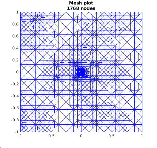
(a) Slit domain adaptive mesh for primal DPG

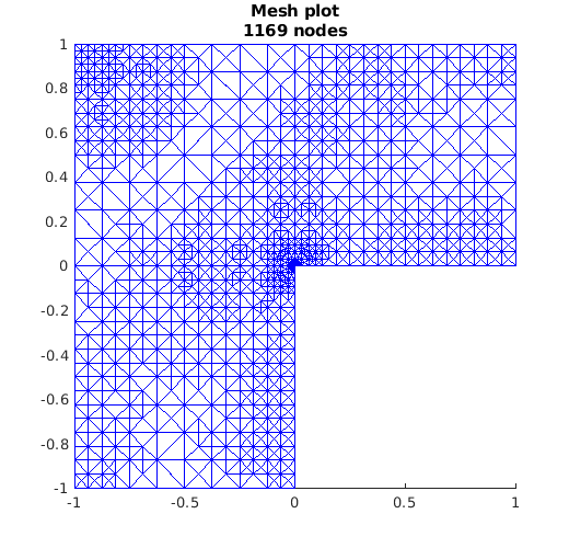
(b) L-shaped domain adaptive mesh for primal DPG

Figure 1. Adaptive meshes after 4 Iterations

5.1. Numerical results on the square domain

Our first domain is the convex square domain, which is defined as $\Omega=[0,1]^{2}$. For this domain the exact solution is well known. Here we compare our solution with the first eigenvalue $\lambda_{1}=2\pi^{2}$. In Figure 2 we can clearly see that the methods show the expected convergence rates.

Figure 2. Convergence rates on the square domain, uniform refinement (p = primal, u = ultra weak)

5.2. Numerical results on the L-shaped domain

On the non-convex L-shaped domain $\Omega=(-1,1)^{2}\setminus\big{(}[0,1)\times(-1,0]\big{)}$ we used the reference values

$$\lambda_{1}=9.639723844871536\ \text{and}\ \lambda_{5}=31.91263.$$

These two eigenvalues correspond to singular eigenspaces that belong to $H^{1+s}(\Omega)$ with $s<1/2$. For this reason we expect a convergence rate of $2/3$ in terms of the number of degrees of freedom when using a uniform mesh refinement. This rate of convergence is clearly detected for $\lambda_{1}$ in Figure 3, while in the case of $\lambda_{5}$ a pre-asymptotic convergence is detected: the rate of convergence is approximately $0.78$ in the last iteration of Figure 4, but it can be seen that the rate is degenerating as the mesh is refined. For bulk parameter $\theta=0.5$ all adaptive methods show optimal convergence rates.

For the higher order methods figure 5 shows a similar behaviour as in the lowest order case. Moreover, the convergence rate can be restored in the adaptive case (Figure 6).

Figure 3. Convergence rates for the L-shaped domain, first eigenvalue

Figure 4. Convergence rates for the L-shaped domain, fifth eigenvalue

Figure 5. Convergence rates for higher order on L-shaped domain (p = primal, u = ultraweak)

Figure 6. Adaptive convergence rates for the L-shaped domain for higher order(p = primal, u = ultraweak)

5.3. Numerical results on the slit domain

On the non-convex slit domain $\Omega=(-1,1)^{2}\setminus\big{(}[0,1)\times\{0\}\big{)}$ we used $\lambda_{1}=8.371329711$ as reference solution. For the first eigenvalue we expect a convergence rate of $1/2$ when the mesh is refined uniformly. Like for the L-shape domain, the adaptive methods can recover the optimal convergence rate.

Figure 7. Convergence rates for the slit domain

5.4. Higher order term

In our next numerical simulation, we check in the lowest order case the statement of Proposition 16 about the higher order term appearing in our a posteriori estimates. In order to calculate the higher order term, we computed a reference solution on a fine mesh with about a million of degrees of freedom. In Figure 8 we can appreciate that the term $\|\lambda u_{0}-\lambda_{h}u_{0,h}\|$ is actually of higher order and converges twice as fast as the eigenfunction in both cases that we have considered. The rate is actually stabilizing about the value of $1$, even if on the slit domain the convergence is faster in the pre-asymptotic regime.

Figure 8. Convergence higher order term

5.5. Efficiency-ratio

Our last numerical test concerns the efficiency-ratio, defined as $\frac{\eta}{\|\tilde{u}-u\|_{U}}$. We used the same reference solution that we computed for the higher order term calculation. In table 5.5 we can see that for the L-shaped domain we have an efficiency-ratio between 9 and 10. For the slit domain we have a ratio between 14 to 19.

[tabular=—l—l——l—l—, table head= DoF Efficiency-ratio (L-shaped) DoF Efficiency-ratio (Slit)
, late after line=
] data/primal_Lshaperatio.csvdof_lshape=, ratio_lshape=, dof_slit=,ratio_slit= $\ratiolshape$ $\ratioslit$

Table 1. Efficiency ratio for primal error estimator $\eta$

References

- [1] I. Babuška and J. Osborn, Eigenvalue problems, Handbook of numerical analysis, Vol. II, Handb. Numer. Anal., II, North-Holland, Amsterdam, 1991, pp. 641–787.
- [2] F. Bertrand and D. Boffi, First order least-squares formulations for eigenvalue problems, (2020), Submitted. arXiv:2002.08145 [math.NA].
- [3] by same author, Least-squares for linear elasticity eigenvalue problem, (2020), Submitted. arXiv:2003.00449 [math.NA].
- [4] D. Boffi, Finite element approximation of eigenvalue problems, Acta Numer. 19 (2010), 1–120. MR 2652780
- [5] T. Bouma, J. Gopalakrishnan, and A. Harb, Convergence rates of the DPG method with reduced test space degree, Comput. Math. Appl. 68 (2014), no. 11, 1550–1561. MR 3279492
- [6] J. Bramwell, L. Demkowicz, J. Gopalakrishnan, and W. Qiu, A locking-free DPG method for linear elasticity with symmetric stresses, Numer. Math. 122 (2012), no. 4, 671–707. MR 2995177
- [7] S. C. Brenner and L. R. Scott, The mathematical theory of finite element methods, Springer New York, 2008.
- [8] T. Bui-Thanh, L. Demkowicz, and O. Ghattas, A unified discontinuous Petrov-Galerkin method and its analysis for Friedrichs’ systems, SIAM J. Numer. Anal. 51 (2013), no. 4, 1933–1958. MR 3072762
- [9] V. M. Calo, N. O. Collier, and A. H. Niemi, Analysis of the discontinuous Petrov-Galerkin method with optimal test functions for the Reissner-Mindlin plate bending model, Comput. Math. Appl. 66 (2014), no. 12, 2570–2586. MR 3128580
- [10] C. Carstensen, L. Demkowicz, and J. Gopalakrishnan, A posteriori error control for DPG methods, SIAM J. Numer. Anal. 52 (2014), no. 3, 1335–1353. MR 3215064
- [11] by same author, Breaking spaces and forms for the DPG method and applications including Maxwell equations, Comput. Math. Appl. 72 (2016), no. 3, 494–522. MR 3521055
- [12] C. Carstensen, M. Feischl, M. Page, and D. Praetorius, Axioms of adaptivity, Comput. Math. Appl. 67 (2014), no. 6, 1195–1253. MR 3170325
- [13] C. Carstensen, D. Gallistl, F. Hellwig, and L. Weggler, Low-order dPG-FEM for an elliptic PDE, Comput. Math. Appl. 68 (2014), no. 11, 1503–1512. MR 3279489
- [14] C. Carstensen and Numerical Analysis Group, AFEM software package and documentation.
- [15] J. Chan, L. Demkowicz, and R. Moser, A DPG method for steady viscous compressible flow, Comput. & Fluids 98 (2014), 69–90. MR 3209958
- [16] L. Demkowicz and J. Gopalakrishnan, A class of discontinuous Petrov-Galerkin methods. Part I: the transport equation, Comput. Methods Appl. Mech. Engrg. 199 (2010), no. 23-24, 1558–1572. MR 2630162
- [17] by same author, Analysis of the DPG method for the Poisson equation, SIAM J. Numer. Anal. 49 (2011), no. 5, 1788–1809. MR 2837484
- [18] by same author, A class of discontinuous Petrov-Galerkin methods. II. Optimal test functions, Numer. Methods Partial Differential Equations 27 (2011), no. 1, 70–105. MR 2743600
- [19] by same author, A primal DPG method without a first-order reformulation, Comput. Math. Appl. 66 (2013), no. 6, 1058–1064. MR 3093480
- [20] L. Demkowicz, J. Gopalakrishnan, and A. H. Niemi, A class of discontinuous Petrov-Galerkin methods. Part III: Adaptivity, Appl. Numer. Math. 62 (2012), no. 4, 396–427. MR 2899253
- [21] T. Führer, Superconvergence in a DPG method for an ultra-weak formulation, Comput. Math. Appl. 75 (2018), no. 5, 1705–1718. MR 3766545
- [22] J. Gopalakrishnan, I. Muga, and N. Olivares, Dispersive and dissipative errors in the DPG method with scaled norms for Helmholtz equation, SIAM J. Sci. Comput. 36 (2014), no. 1, A20–A39. MR 3148088
- [23] J. Gopalakrishnan and W. Qiu, An analysis of the practical DPG method, Math. Comp. 83 (2014), no. 286, 537–552. MR 3143683
- [24] F. Hellwig, Adaptive discontinuous Petrov–Galerkin finite-element-methods, Ph.D. thesis, Humboldt-Universität zu Berlin, Mathematisch-Naturwissenschaftliche Fakultät, 2019.
- [25] N. V. Roberts, T. Bui-Thanh, and L. Demkowicz, The DPG method for the Stokes problem, Comput. Math. Appl. 67 (2014), no. 4, 966–995. MR 3163889
- [26] N. V. Roberts, L. Demkowicz, and R. Moser, A discontinuous Petrov-Galerkin methodology for adaptive solutions to the incompressible Navier-Stokes equations, J. Comput. Phys. 301 (2015), 456–483. MR 3402741
- [27] J Schöberl, NETGEN an advancing front 2d/3d-mesh generator based on abstract rules, Computing and Visualization in Science 1 (1997), no. 1, 41–52.
- [28] by same author, C++ 11 implementation of finite elements in ngsolve, Institute for Analysisand Scientific Computing, Vienna University of Technology (2014).
- [29] J. Zitelli, I. Muga, L. Demkowicz, J. Gopalakrishnan, D. Pardo, and V. M. Calo, A class of discontinuous Petrov-Galerkin methods. Part IV: the optimal test norm and time-harmonic wave propagation in 1D, J. Comput. Phys. 230 (2011), no. 7, 2406–2432. MR 2772923