Extrapolating from neural network models: a cautionary tale

Abstract

We present three different methods to estimate error bars on the predictions made using a neural network. All of them represent lower bounds for the extrapolation errors. For example, we did not include an analysis on robustness against small perturbations of the input data.

At first, we illustrate the methods through a simple toy model, then, we apply them to some realistic cases related to nuclear masses. By using theoretical data simulated either with a liquid-drop model or a Skyrme energy density functional, we benchmark the extrapolation performance of the neural network in regions of the Segrè chart far away from the ones used for the training and validation. Finally, we discuss how error bars can help identifying when the extrapolation becomes too uncertain and thus unreliable.

I Introduction

Neural networks Friedman et al. (2001) (NN) are powerful tools that are widely used in several domains of science. Within the nuclear physics community, several groups have started investigating the NN as a tool to improve current models in predicting specific observables such as nuclear masses Utama et al. (2016); Utama and Piekarewicz (2017); Neufcourt et al. (2018); Pastore et al. (2020) and radii Akkoyun et al. (2013), or as intermediate tool to avoid time-consuming calculations Lasseri et al. (2020). The domain of application is so vast since NN are universal approximators Cybenko (1989): any continuous function can be approximated by a single-layer neural network with a sufficiently large number of neurons. Each neuron forming the NN contains some adjustable (hyper-)parameters (weights and biases) that are determined in order to minimise a given objective or loss function, typically the mean squared error.

Once the architecture of the network is fixed, i.e. the number of layers, nodes and the connection patterns, the critical aspect is to find the optimal set of data to optimise the values of the weights and biases. To some extent, this is the same procedure commonly used in nuclear physics to adjust model parameters Kortelainen et al. (2010, 2014). As a consequence, it is important to equip the NN with a reasonable estimate of the error bars to help assessing the quality of the results.

As discussed in Ref.Dobaczewski et al. (2014), estimating theoretical errors is not an easy task since many factors could contribute to them. In particular, one can model the prediction error in terms of two main components: a statistical and a systematic one. The first arises from the optimisation procedure and it can be evaluated using specific statistical tools, while the second is usually unknown.

The standard strategy used to estimate error bars is based on the covariance matrix and the first derivative of the model in parameter space. See Refs.Dobaczewski et al. (2014); Roca-Maza et al. (2015) for more details. Such an operation can not be applied to a typical NN for a very simple reason: the number of parameters is very large, typically in the range of thousands. Since the NN is non-linear in parameter space Barlow (1989), it follows that the covariance matrix need to be evaluated by performing numerical derivatives in the parameter space. Due to the possible numerical issues discussed in Ref. Roca-Maza et al. (2015), we prefer not to explore this method.

In the present article, we study three different methods to estimate error bars that do not require major modification to the existing Python functions. To this purpose, we train a series of NNs using nuclear mass data derived from existing nuclear models: the liquid-drop (LD)Weizsäcker (1935) and the Skyrme nuclear energy density function (NEDF) Bender et al. (2003). The idea is very simple: guided by the current knowledge of nuclear masses Wang et al. (2017), we separate our theoretical masses in two sets: one corresponding to the measured ones ($\approx 2400$ nuclei) and the other corresponding to the extrapolated region. This mimic the current situation when in the scientific literature several authors try to extrapolate models in regions where no data are available. The choice of using data generated through models and not experimental values is dictated by the desire of working on systems for which the values of the mass is available, to assess the validity of the error bars. We are aware that the trained NN will not produce meaningful estimations for nuclei. The best that can be achieved is to approximate the explicit formula of the model (say, Liquid Drop) through the NN.

Our goal it to show that even this simple approximation is challenging, and that extrapolation can be at best attempted close to the region of the known nuclear masses.

The article has been structured to be used as a guide to navigate the associated Jupiter notebooks made available as Supplementary material. The article is organised as follow: in SecII we briefly introduce the NN and its error estimate and we apply it to a simple toy-model; in Sec.III we present the nuclear models we use to obtain the data-set; in Sec.IV we discuss the various methods to estimate error bars applied to realistic cases. Finally, we present our conclusions in Sec.V.

II What is a Neural Network?

A Neural Network Friedman et al. (2001) is an ensemble of elementary units called neurons arranged in layers and connected to each other. The individual neuron is represented mathematically as an activation function $f$ (representing a neuron action potential), that takes some weighted inputs and sums them up to produce an output. In a formula, the output $y$ of a neuron is

$$y=f(\mathbf{x}\cdot\mathbf{w}+b)\;,$$ (1)

where $\mathbf{x}$ is the input vector, $\mathbf{w}$ is the vector of weights and $b$ the bias. The values of $\mathbf{w}$ and $b$ are not known and they need to be determined by training the network. The goal of the training process is to minimise the mean squared error (MSE)

$$MSE=\frac{1}{N}\sum_{i=1}^{N}\left(Y_{i}-\hat{Y}_{i}\right)^{2},$$ (2)

where $N$ is the number of observations used to train the network, $\hat{Y}_{i}$ is the prediction of the network for observation $i$ while $Y_{i}$ is the actual value for observation $i$. Notice that $Y$ can be the result of an experiment or of a theoretical calculation.

A feed-forward single-layer neural networks with a non-polynomial activating function can approximate any function Leshno et al. (1993): the quality of the approximation will depend on the number of neurons, but also to some extent on the adopted training procedure Ruder (2016) or even the initialisation for weights and biases Mishkin and Matas (2015). The theorem given in Ref.Leshno et al. (1993) is independent on the details of the training procedure. However, the time required to train a large neural network can be prohibitive and the scarcity of data can limit the applications of NN. It is thus important to train the NN using the best features in order to maximise the quantity of information one can extract from the data. See discussion in Ref. Carnini and Pastore (2020) for more details.

To better illustrate such a concept, we present a simple toy-model. The calculations were performed using a Jupiter notebook that is provided as a Supplementary Material. The application of NN to the nuclear case starts at Sec.III.

II.1 Fitting a parabola

We generate 100 points in the interval $x\in[0,1]$ and evaluate the function $Y(x)=x^{2}$ . We split the data set into a training and validation as 80% and 20% of the data. For the purpose of this example, we build a single layer NN using 8 neurons. We selected the rectified linear (ReLu) $f(x)=max(0,x)$ Karlik and Olgac (2011); Lu et al. (2017) as activation function. This is a quite popular choice since it allows to train networks with several layers without incurring in gradient vanishing problems. The weights are initialised using a glorot uniform Glorot and Bengio (2010), i.e. they are drawn from a truncated uniform distribution. This is the default option for the Dense function in Keras Chollet (2017). Different initialiser could be used with more stringent assumptions on the structure of the weights, here we use a simple Bayesian approach: since we have no prior knowledge of the weights, we use a simple uniform distribution.

After training the NN over 2000 epochs, we obtain the result given in the left panel of Fig.1. We observe that the network is capable to grasp the structure of the data. The mean square error, Eq.2, on the training set is $\approx 5\cdot 10^{-5}$. For this particular case, the MSE on the validation is also very similar showing that the NN provides a very good approximation of the data.

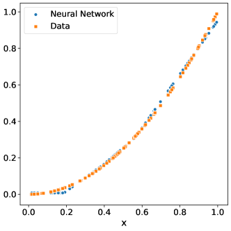
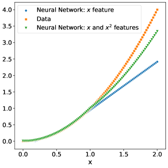
Figure 1: Left: comparison between Neural Network interpolation (circles) and the original data points of the model (squares). Right: comparison between Neural Network extrapolations with (lower triangles) and without additional features (circles) and data points extracted from the original function $Y(x)=x^{2}$ (squares). See text for details.

However, it is worth investigating what happens when we extrapolate using the NN in a region of space where there are no training data. In the right panel of Fig.1, we illustrate the extrapolation of the NN in the interval $x\in[1,2]$ and we compare it with the true model $Y(x)=x^{2}$. We see that the extrapolation quickly deteriorates and eventually the difference between true model and NN quickly increases. In particular, we notice that the NN is not able to capture the quadratic behavior of the data and we see a clear linear dependence in the region of the extrapolation, a side effect of choosing ReLU as an activation function.

NN can learn any type of structure in the data Leshno et al. (1993), but we can help the network by providing extra information, exactly in the same way as we did in Ref. Carnini and Pastore (2020). In data science lexicon, this is called feature engineering. The role of feature engineering is to improve the predictions obtained with the NN without increasing the number of data or changing its architecture.

For this example, we train a new NN using exactly the same layout, but now including as input data both $x$ and $x^{2}$. In this case, we know the exact structure of the toy model, but in a realistic case one should explore various possibilities.

We stress that we are not changing the data, but we are simply making a transformation to highlight possible patterns in the training set. In other terms, we are only adapting the data representation given to the algorithm (NN) that we chose. For example, including $x^{2}$ would not alter significantly the performance of a Decision Tree  Carnini and Pastore (2020).

In the right panel of Fig.1, we compare the trained network with the additional feature $x^{2}$ (triangles) to the simpler NN (full circles). In the region $x\in[0,1]$ both NN do very well, but the one using additional features clearly behaves way better in the interval $x\in(1,2]$.

Finding the most relevant feature to improve the quality of the network during the training process is not an easy task. It is thus important to assess the quality of the NN, by defining error bars that may guide us in evaluating the quality of an extrapolation in a realistic case, where we do not know the structure of the exact model. Finally, it is worth mentioning that adding features that are not relevant for the model could actually lead to a deterioration of the results. See the discussion in Ref.Brownlee (2020).

II.2 Error bars

Within scientific literature there is no consensus on how to estimate error bars for NN. The standard approach based on the covariance matrix Dobaczewski et al. (2014) can not be applied due to the typical large number of parameters and the clear difficulties in performing numerical derivatives in parameter space Roca-Maza et al. (2015); Shelley et al. (2019). In the following, we investigate three possible methods using the example illustrated in Sec.II.1. For simplicity we consider $x$ as the only feature to train the network.

II.2.1 Epoch averaging

During the training of a NN, it is possible to store its coefficients at fixed values of epochs during the training Brownlee (2018). The approach was introduced independently by Polyak Polyak (1990); Polyak and Juditsky (1992) and Ruppert Ruppert (1988), and in also known as Polyak or Polyak-Ruppert averaging. In the case of this toy model, there is no variability, since the coefficients converge to their final result after few epochs and the gradient vanishes (see the Supplemental material). In a realistic case, as shown in Fig.3, one observes that the MSE as a function of epochs decreases till reaching a plateau where it starts fluctuating since the gradient does not reach a stable minimum. This means that the coefficients of the network are still slightly varying as a function of the epochs. By storing them, for example, every 1000 epochs, we effectively create different networks with similar MSE. Having access to the different networks, we define the error bar in a statistical way as the interval where 68% of predictions lie.

The main advantage of this method is that we do not need to train additional networks and thus it is a remarkable gain in CPU/GPU time. The downside is that all these networks are not independent from one another, but they typically manifest a strong degree of correlation and thus leading to an underestimation of the error bars. The additional downside is that if the gradient vanishes during the training, the NN gets to a stable configuration and as such averaging over successive epochs does not introduce any variability. This would also lead to an underestimation of the error bars.

II.2.2 Bootstrap

A very simple alternative to the epoch averaging is based on bootstrap Efron and Tibshirani (1986); Pastore (2019). Since the training of a network is essentially a non-linear fit, we can explore the landscape of parameter space by using slightly different training sets. To this purpose, given the data, we create 100 sets of validation/training sets, by random sampling the original one. For each of them, we train a NN with the same architecture. We see that each individual network will be trained only on a fraction of the total data (here 80%), but the full ensemble will be trained over all the data. As a consequence, using bootstrap, we maximise the information contained in the data. Having access to 100 networks, we average them out and define an error bar as the region where 68% of the curves lie, while the expected prediction is obtained by simply averaging out the outcomes of all NNs.

In the left plot of Fig.2, we show the resulting prediction obtained using the bootstrap method: we see that the error bars are very small in the region $[0,1]$ while they grow when $x$ approaches the limits of the data set. Beyond $x=1$, the error bars grow remarkably fast, as expected due to the lack of information in this region of space.

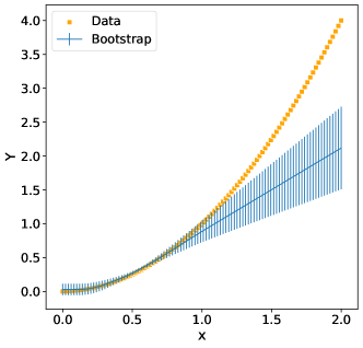
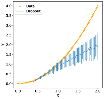
Figure 2: Left: comparison between Neural Network using bootstrap (solid line) and the original data (squares). Right: comparison between Neural Network using dropout (solid line) and the original data (squares). See text for details.

The error bars obtained with bootstrap strongly depend on the variability of the predictions. By investigating in more detail the left plot of Fig.2, we observe that the true model falls within the error bars only up to $x\approx 1.25$. To go beyond this point one should use larger error bars by taking, for example, two standard deviations, but one clearly notices that this makes the prediction less and less relevant given the size of the error bars.

II.2.3 Dropout

Finally, we consider the dropout method to estimate the error bars. This is a technique that has been introduced to avoid over-fitting and to improve predictions. The idea is very simple Srivastava et al. (2014): we train the network over the training set and we randomly switch off some neurons. In this simple toy model we turn off 1 neuron each time.

We call the trained NN 100 times allowing to switch off one neuron randomly each time. In this way we produce 100 predictions and we define the error bar, as in the bootstrap case, as the region where 68% of the predictions lie. The result is illustrated in the right plot of Fig.2.

By comparing the results for bootstrap and dropout in Fig.2, we see that the dropout gives very similar results to the bootstrap case. The error bars estimated in this way contain the true model up to $x\approx 1.25$. Beyond this point although the error bars continue growing, the difference between the model and the prediction is clearly under-estimated by our error bars.

We now move to some realistic nuclear data to continue testing the three methods presented here to evaluate error bars.

III Nuclear masses

Currently Wang et al. (2017), more than 2400 nuclear masses have been experimentally measured with very high degree of accuracy. The exact knowledge of nuclear binding energies play a crucial role in several physical scenarios as for example r-process nucleosynthesis Cowan et al. (1991) or in the determination of the chemical composition of the crust of a neutron star Chamel and Haensel (2008). Since NN have been recently applied to perform extrapolations of nuclear masses Utama et al. (2016); Utama and Piekarewicz (2017); Neufcourt et al. (2018); Pastore et al. (2020) in regions where no experimental data are still available, we find very important to provide a reliable estimate of the error bars to help evaluating the quality of such results.

As done in the previous section, we validate the quality of the extrapolation against a closed-form model. To this purpose, instead of using experimental masses, we use binding energies extracted from a nuclear model. The synthetic data are generated using a liquid-drop model Pastore (2019) and the NEDF via the Skyrme SLy4 parametrisation Chabanat et al. (1998); Stoitsov et al. (2006). Both LD and SLy4 give a reasonable reproduction of nuclear binding energies, with an RMS of few MeV. Other mass-models with improved accuracy are available within the literature Goriely et al. (2009); Duflo and Zuker (1995); Moeller and Nix (1994); Sobiczewski and Litvinov (2014), but – for the present calculation – we are only interested in considering two categories of models: one linear and the other non-linear, just to check if the performances of the NN are impacted by such a choice.

Both LD and SLy4 predict the existence of way more nuclei than the one experimentally observed Wang et al. (2017) and they allow us to perform benchmark against NN predictions along several complete isotopic chains.

To be as realistic as possible, we define for the training set of the NN all the measured isotopes given in Ref Wang et al. (2012), but using the values of binding energies calculated by the models. We stress that at this stage, we are not interested in reproducing as accurately as possible experimental data, but to validate the approach for extrapolations based on NN.

We build a NN formed by 3 layers having 16-8-16 neurons respectively densely connected and using a ReLu activation function. No particular effort was dedicated to fine tune and optimise the architecture, except for fixing reasonable defaults (see for example Lu et al. (2017)). Following Ref. Anil et al. (2020), the NN is directly trained on total binding energies per particle to avoid any additional bias introduced by the model itself.

III.1 Liquid Drop data

The LD model express the nuclear binding energy,$B$, as a sum of five different terms depending uniquely on proton ($Z$) and neutron ($N$) number as

$$\frac{B^{LD}(N,Z)}{A}=a_{v}-a_{s}A^{-1/3}-a_{c}\frac{Z(Z-1)}{A^{4/3}}-a_{a}\frac{(N-Z)^{2}}{A^{2}}-\delta\frac{mod(Z,2)+mod(N,2)-1}{A^{3/2}}$$ (3)

where $A=N+Z$ and the coefficients $a_{v},a_{s},\dots$ have been adjusted in Ref. Pastore (2019). The features of the model are quite simple and one could use them to directly train the network Carnini and Pastore (2020). However, here we consider no a priori knowledge of the model and we use only $N$ and $Z$ as features.

In Fig.3, we show the evolution of the RMS (expressed in MeV) as a function of the epochs, for both training and validation sets. We used as a label the energy per particle $B/A$ given by Eq.3. The motivation for our simple choice of the network can be seen here: after few thousands of epochs, the network has reached a plateau, where the gradient is small. The fast convergence is a necessary ingredient for our successive analysis on error bars.

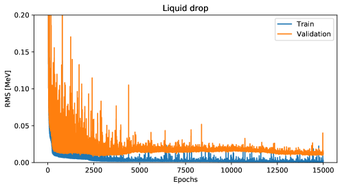
Figure 3: Evolution of the root mean square, Eq.2, as a function of the epochs used for training the NN and based on LD data. See text for details.

The final RMS on the training set is $\sigma_{tr}\approx 50$ keV, while on the validation is $\sigma_{val}\approx 100$ keV. The accuracy is roughly of the same order of magnitude of the LD respect to experimental nuclear data. By training a second NN on the residuals it would be probably possible to further reduce the RMS Anil et al. (2020), but this is not the goal of the present discussion. We want to stress here that the NN trained here is probably not the best one we can build out of the data, but a reasonable tool that we can use for our analysis on error bars.

Having trained the NN, we define the residuals as the difference between the $B^{LD}/A$ and the binding energy per particle as calculated via the NN $B^{NN}/A$. In Fig.4, we compare the evolution of the residuals as a function of the mass number $A$ for two isotopic chains: Calcium and Lead. The choice of the isotopic chains is somehow arbitrary: we picked those to illustrate that there is no difference when selecting a light or an heavy element.

To guide the eye, we have added an horizontal line to indicate the position of zero. The vertical dashed line indicates the position of the heaviest isotope used to train the network. The first estimate of the error of the NN is represented by its RMS. Assuming that the errors are normal, we set the error bar Barlow (1989) to 1$\sigma$, equal to the global RMS of the model on the validation set, as done in Ref. Pastore et al. (2020).

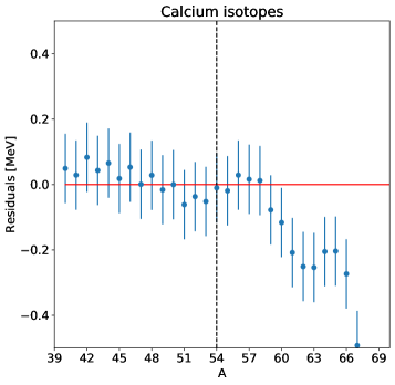
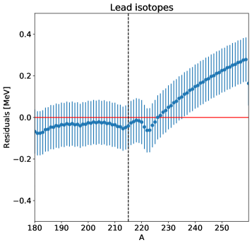
Figure 4: Evolution of the difference between the energy per particle calculated using the LD model and the NN. The vertical dashed line indicates the position of the last isotope used to train the NN. The horizontal line indicates the zero and it helps guiding the eye. See text for details.

The simple error bar used here can be considered probably as a very good approximation to compare with data within the range of the training, i.e. in this case for Calcium isotopes with $A\leq 54$ and $A\leq 215$ for lead isotopes, while it clearly underestimates the real statistical error in the extrapolation region. The result shown in Fig.4, especially in the extrapolated region, is very much dependent on several quantities as the initialisation of the weights or a different splitting of the data in training/validation. As such, the naïve extrapolation done here can not be considered as reliable even if accidentally some of the nuclei in the extrapolated region are still well reproduced.

A more refined error bar, based on the methodologies of Sec.II.1 is presented in Sec.IV.

III.2 Skyrme data

Within the NEDF theory, the total binding energy of a nucleus is written as the space integral of an energy density functional obtained using a microscopic Skyrme interaction Perlińska et al. (2004); Becker et al. (2017). Differently from LD, the Skyrme model is non linear in parameter space, since all the densities appearing in the various terms of the functional Tondeur (1983) are obtained as a self-consistent solution of the Hartree-Fock-Bogoliubov equations using an iterative procedure Ring and Schuck (2004). In the present article, we consider the data calculated in Ref. Stoitsov et al. (2006) using the SLy4 functional Chabanat et al. (1998).

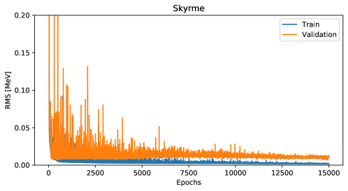
Figure 5: Same as Fig.3, but using SLy4 data.

From the statistical point of view, the interest in using a microscopic calculation is related to the fact that the features are not so evident as in the case of the LD model shown in Eq.3, although the overall quality is reproducing nuclear masses is similar.

Following the same procedure used for LD, we now train a NN over Skyrme data with the same layout. In Fig.5, we illustrate the evolution of the RMS as a function of the number of epochs used for the training. As discussed previously, the goal of the current paper is not to find the optimal NN, but to discuss the optimal methodology to estimate error bars.

After 15000 epochs, we obtain an RMS of $\sigma_{tr}=\approx 50$ keV on the energy per particle for the training and $\sigma_{val}=\approx 100$ keV for the validation set. These performances are comparable to the one of the NN trained on the LD data.

In Fig.6, we show the evolution of the NN predictions along the isotopic chain of Calcium and Lead, in the same way as we did in Fig.4. Although the drip-lines obtained using LD and SLy4 are not equal, we observe that our NN behaves quite nicely for the first isotopes beyond the last known nucleus and then it diverges.

The simple error estimate based on the RMS clearly under-estimate the true error, although by chance the Lead isotopes are very well reproduced by our NN in the extrapolated region.

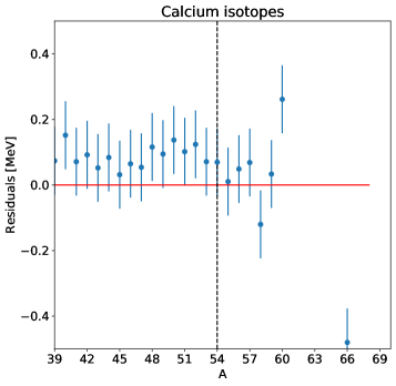
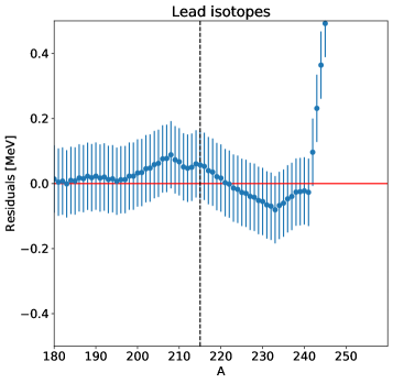
Figure 6: Same as Fig.4, but for SLy4 data

IV Error estimate

In this section, we apply the three different methods discussed in Sec.II.1 to the realistic data obtained from LD and Skyrme-SLy4 models.

IV.1 Epoch-averaging

By looking at Fig.3 and Fig.5, we observe that both loss functions reach a plateau region around 10000 epochs. The gradient is not zero and we still observe small fluctuations. This means that the weights and the biases of the NN are still fluctuating as a function of the epochs, although we expect these fluctuations to be small.

We take advantage of the epoch-averaging idea presented in Sec.7,by continue the training and store the weights every 1000 epochs for 100 times. We create 100 models with all slightly different parameters, but using exactly the same data set for training and validation.

We define an average model, by calculating the mean value of the models and the 1-$\sigma$ error as the region containing 68% of the predictions. The result is presented in Fig.7 for Ca and Pb isotopic chains using the synthetic data calculated using LD and Skyrme. The vertical lines indicate the position of the last experimentally known nucleus in the chain.

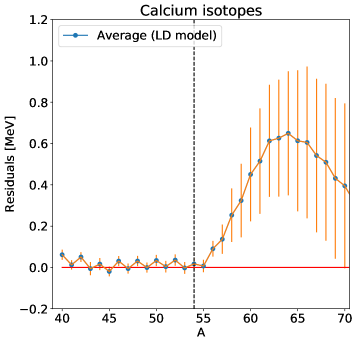
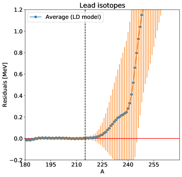
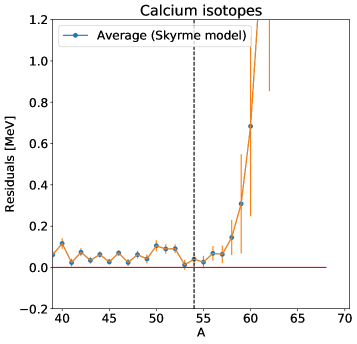
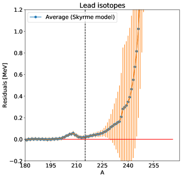
Figure 7: Same as Fig.4, but using epoch-averaging to estimate error bars. On the left panels calcium isotopes and on the right panels the lead isotopes. The top row has been obtained using LD data, while the bottom row using Skyrme data. See text for details.

We observe that the error bar is very small in the region where data are present (the training set). This value is even smaller than the naïve RMS shown in Figs.4-6. In the region of extrapolation, i.e $A\geq 54$ for calcium isotopes and $A\geq 215$ for lead, the error bars start to grow quite fast becoming soon way larger than the simple RMS. The predictions done with the NN are reasonable for isotopes with few neutrons beyond the vertical line, but the prediction quickly deteriorates and the uncertainties becomes soon very large, and in clear disagreement with the true model.

Although such a procedure is quite simple and not too expensive in terms of CPU/GPU, it is worth recalling that the different networks are not independent from one another, but they are highly correlated. This can be checked by evaluating the correlation matrix between them. The consequence is that changing the training set will lead to a different prediction and different error bars. Although the main outcome will remain the same.

IV.2 Bootstrap

A different approach to avoid the strong dependence on the training set is based on the bootstrap method Efron and Tibshirani (1986); Pastore (2019). In this case, we randomly split the available data into training and validation, reshuffling them at each bootstrap iteration. By using 100 bootstrap iterations, we have thus obtained 100 neural networks, all trained for the same amount of epochs (15000). By visually inspecting the evolution of the RMS, we have checked that all networks have reached convergence with a final RMS on the training and validation set of the same quality of the original one. As done before, we calculate the average and the variance of the various neural networks to define an error bar. In this case, by examining the correlation matrix, one observes still a correlation, but much weaker than in the previous case of epoch averaging. The different NN are still partially correlated since they have been trained to strongly overlapping data-sets.

In Fig.8, we illustrate the evolution of the difference between the energy per particle as calculated with the LD and Skyrme models using the NN, together with the associated error bar trained using the bootstrap method.

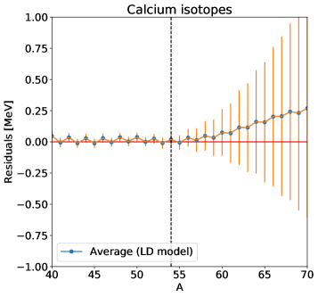
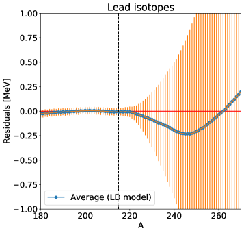
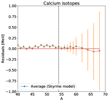
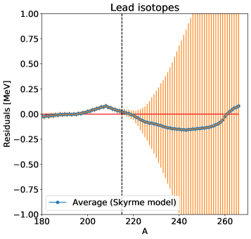
Figure 8: Same as Fig.4, but using bootstrap to estimate error bars. See text for details.

The error bars obtained with bootstrap are robust, i.e. they do not depend on the particular choice of the initial data-set, but they seem to overestimate the real precision of the NN. By moving few isotopes beyond $A=215$ for Pb and $A=54$ for Ca, the error grows fast and they soon reach several hundreds of keV. From the statistical point of view this error bar can be seen as a very conservative estimate of the predictive power of the model since the true model is always included within these error bars. This was not the case of epoch-averaging as shown in Fig.7.

IV.3 Dropout

We now consider the third method to estimate error bars and based on dropout Srivastava et al. (2014). As explained in detail in the simple toy-model example, during the training of the NN, we randomly turn off a given percentage of neurons for the predictions. This procedure is used in the literature to check the robustness of the network and to avoid over-fitting of the weights. As discussed in Ref. Srivastava et al. (2014), dropout can be used as an approximation to a more involved Bayesian Neural Network (BNN). The main advantage of dropout compared to BNN is that the typical training time required to determine the weights is shorter. To mimic BNN, we apply the same dropout also to the prediction. This means that every time we call the NN to obtain a value, we randomly turn off a set of neurons. This will give us the required variability to estimate an error. For simplicity (namely, writing the least amount of code), we used the option from Keras Chollet (2017); Chollet et al. (2015) to use dropout at both training and prediction phases.

The layout of the NN is the same of previous cases, but we had to increase the number of epochs to 30000 to let the gradient get to a stable plateau. The drop-out rate is arbitrary, for the present calculation we have used a rate of 5%. Other rates could be explored, but given the architecture of the NN and the relatively small number of neurons, higher dropout would lead to very poor performances. In the present case, using 5% dropout, the resulting root mean square is of $\approx 150$ keV for both the training and the validation set. This value is roughly 3 times worst than what we obtained using the same layout without dropout.

During the training phase, some neurons are silenced, forcing the other neurons to learn to compensate the missing ones. By spreading the information learned by one neuron to another, the dropout effectively improves the performance by assembling the predictions of different models trained in parallel. By default, the dropout is not used during the predictions, and the output of all neurons is considered. In this way, the prediction process is deterministic and reproducible.

If, however, the dropout is used at prediction time, every time a prediction is launched a different result is possible. This leads to a distribution function for each and every prediction. If we assume a normal distribution, by averaging and taking the standard deviation an estimation with a bar error can be obtained. Of course, the normal distribution is not strictly required, but in order to assess the root mean square $\sigma$, the second momentum should be finite.

With a finite amount of neurons, the possible outcomes are limited: for a neural network with 10 neurons and a drop out rate of 10%, every time a prediction is made one of the neurons is silenced. This lead to only ten possible distinct values for the prediction.

The result is reported in Fig.9 for the two data-sets used and for two isotopic chains. The quality of the predictions in the region used for the training is slightly worst, but in the extrapolated region we observe that the behavior of the resulting error bar is somehow intermediate between the epoch-averaging and the bootstrap.

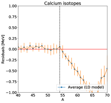
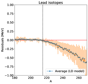
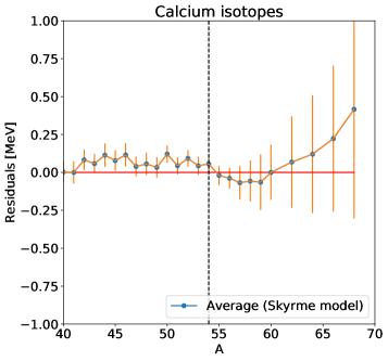
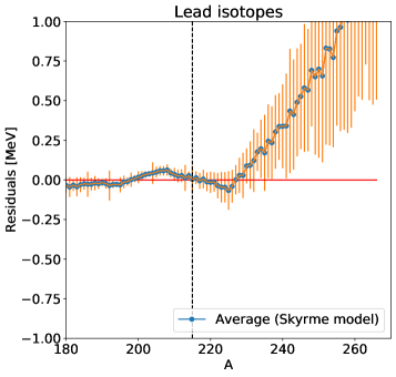
Figure 9: Same as Fig.4, but using dropout to estimate error bars. See text for details.

Similarly to the bootstrap case, the use of dropout reduces the dependence of the outcome on the specific choice of training/validation set, but using much less CPU time. The error bars contain the true model only for few isotopes beyond the last known nucleus in the LD model, while for the Skyrme model the error bars do a better job. This may be accidental and not easy to predict without knowing the true model.

V Conclusions

We have presented three different methodologies to estimate the error bars of the prediction obtained with a neural network. Through a simple toy-example, we have illustrated in detail the calculations of error bars using epoch-averaging, bootstrapping and dropout. We have applied these three methods to the more realistic case of nuclear binding energies. To benchmark the accuracy of the error bars and predictions, we have used synthetic data obtained from two well known models: the liquid drop and the Skyrme SLy4. By observing the quality of the predictions and the structure of the error bars on two representative isotopic chains, we conclude that bootstrap and dropout are robust methods since they do not depend too much on the particular choice of the initial training set as in the case of epoch-averaging. The bootstrap tends to provide the largest error bars that contains the true value of a large set of nuclei, unfortunately these error bars are so large that the prediction itself lacks any relevance. The dropout seems more promising in providing a more reasonable error bar. Moreover, it has an actual regularisation effect during the training phase thus reducing the difference between the performance on the training and the validation set. The effect during the prediction phase is to lead to a distribution for the predictions. This allows an a posteriori analysis of the results, and thus an error estimation. This mimic the behavior of a more complex Bayesian Neural Network with a reduced computational cost. The optimal dropout rate for training and prediction has not been explored in detail and a relevant study, with some additional programming effort, on the dependence of error bars and, more generally, on the extrapolation performances is required.

Other parameters may also increase the variability of our predictions, as for example the initialisation of the weights. Different choices of weights may lead to slightly different results and they should also be taken into account for a more detailed analysis.

We consider that these results are a first step towards a Machine Learning model for predicting the nuclear masses based on the available, experimental masses. The key ingredients for these models are robust error estimations and validation schemes as discussed in this paper.

Another ingredient that is required for good performance and to generalise beyond the known masses is a solid Feature Engineering approach. We illustrated with the toy model how the usage of the right feature can dramatically improve the predictions. While the example may seem artificial, it serves the purpose to express the need to carefully designed features. This means that neural network can not replace modelling, but only complement it.

VI Acknowledgement

The authors thank R. Lasseri for useful discussions in the initial phase of this work. We also thank M. Shelley and D. Regnier for useful comments. This work has been supported by STFC Grant No. ST/P003885/1.

References

- Friedman et al. (2001) J. Friedman, T. Hastie, and R. Tibshirani, The elements of statistical learning (Springer series in statistics New York, 2001), ISBN 978-0387848570.
- Utama et al. (2016) R. Utama, J. Piekarewicz, and H. Prosper, Physical Review C 93, 014311 (2016).
- Utama and Piekarewicz (2017) R. Utama and J. Piekarewicz, Physical Review C 96, 044308 (2017).
- Neufcourt et al. (2018) L. Neufcourt, Y. Cao, W. Nazarewicz, F. Viens, et al., Physical Review C 98, 034318 (2018).
- Pastore et al. (2020) A. Pastore, D. Neill, H. Powell, K. Medler, and C. Barton, Physical Review C 101, 035804 (2020).
- Akkoyun et al. (2013) S. Akkoyun, T. Bayram, S. O. Kara, and A. Sinan, Journal of Physics G: Nuclear and Particle Physics 40, 055106 (2013).
- Lasseri et al. (2020) R.-D. Lasseri, D. Regnier, J.-P. Ebran, and A. Penon, Physical Review Letters 124, 162502 (2020).
- Cybenko (1989) G. Cybenko, Mathematics of control, signals and systems 2, 303 (1989).
- Kortelainen et al. (2010) M. Kortelainen, T. Lesinski, J. Moré, W. Nazarewicz, J. Sarich, N. Schunck, M. Stoitsov, and S. Wild, Physical Review C 82, 024313 (2010).
- Kortelainen et al. (2014) M. Kortelainen, J. McDonnell, W. Nazarewicz, E. Olsen, P.-G. Reinhard, J. Sarich, N. Schunck, S. Wild, D. Davesne, J. Erler, et al., Physical Review C 89, 054314 (2014).
- Dobaczewski et al. (2014) J. Dobaczewski, W. Nazarewicz, and P. Reinhard, Journal of Physics G: Nuclear and Particle Physics 41, 074001 (2014).
- Roca-Maza et al. (2015) X. Roca-Maza, N. Paar, and G. Colo, Journal of Physics G: Nuclear and Particle Physics 42, 034033 (2015).
- Barlow (1989) R. Barlow, The Manchester Physics Series, New York: Wiley, 1989 (1989).
- Weizsäcker (1935) C. v. Weizsäcker, Zeitschrift für Physik 96, 431 (1935).
- Bender et al. (2003) M. Bender, P.-H. Heenen, and P.-G. Reinhard, Reviews of Modern Physics 75, 121 (2003).
- Wang et al. (2017) M. Wang, G. Audi, F. Kondev, W. Huang, S. Naimi, and X. Xu, Chinese Physics C 41, 030003 (2017).
- Leshno et al. (1993) M. Leshno, V. Y. Lin, A. Pinkus, and S. Schocken, Neural Networks 6, 861 (1993), ISSN 0893-6080, URL http://www.sciencedirect.com/science/article/pii/S0893608005801315.
- Ruder (2016) S. Ruder, ArXiv abs/1609.04747, 1 (2016), retrieved on 10/03/2020, URL https://tinyurl.com/y7b8jxe4.
- Mishkin and Matas (2015) D. Mishkin and J. Matas, ArXiv abs/1511.06422, 1 (2015), retrieved on 24/04/2020, URL https://tinyurl.com/ybjon4eg.
- Carnini and Pastore (2020) M. Carnini and A. Pastore, Journal of Physics G: Nuclear and Particle Physics (2020).
- Karlik and Olgac (2011) B. Karlik and A. V. Olgac, International Journal of Artificial Intelligence and Expert Systems 1, 111 (2011).
- Lu et al. (2017) Z. Lu, H. Pu, F. Wang, Z. Hu, and L. Wang, arXiv 1709.02540, 1 (2017).
- Glorot and Bengio (2010) X. Glorot and Y. Bengio, in Proceedings of the thirteenth international conference on artificial intelligence and statistics (2010), pp. 249–256.
- Chollet (2017) F. Chollet, Deep Learning with Python (Manning Publications, 2017), 1st ed., ISBN 978-1617294433.
- Brownlee (2020) J. Brownlee, Machine learning mastery with Python, https://machinelearningmastery.com/machine-learning-with-python/ (2020).
- Shelley et al. (2019) M. G. E. Shelley, P. Becker, A. Gration, and A. Pastore, Acta Physica Polonica B (2019).
- Brownlee (2018) J. Brownlee, Better Deep Learning, https://machinelearningmastery.com/better-deep-learning/ (2018).
- Polyak (1990) B. Polyak, Avtomatica i Telemekhanika 7, 98 (1990).
- Polyak and Juditsky (1992) B. Polyak and A. B. Juditsky, SIAM Journal of control and optimization 30, 838 (1992).
- Ruppert (1988) D. Ruppert, Tech. Rep., Cornell University (1988).
- Efron and Tibshirani (1986) B. Efron and R. Tibshirani, Statistical science pp. 54–75 (1986).
- Pastore (2019) A. Pastore, Journal of Physics G: Nuclear and Particle Physics 46, 052001 (2019).
- Srivastava et al. (2014) N. Srivastava, G. Hinton, A. Krizhevsky, I. Sutskever, and R. Salakhutdinov, The journal of machine learning research 15, 1929 (2014).
- Cowan et al. (1991) J. J. Cowan, F.-K. Thielemann, and J. W. Truran, Physics Reports 208, 267 (1991).
- Chamel and Haensel (2008) N. Chamel and P. Haensel, Living Reviews in relativity 11, 10 (2008).
- Chabanat et al. (1998) E. Chabanat, P. Bonche, P. Haensel, J. Meyer, and R. Schaeffer, Nuclear Physics A 635, 231 (1998).
- Stoitsov et al. (2006) M. Stoitsov, J. Dobaczewski, W. Nazarewicz, and P. Borycki, International Journal of Mass Spectrometry 251, 243 (2006).
- Goriely et al. (2009) S. Goriely, S. Hilaire, M. Girod, and S. Péru, Physical review letters 102, 242501 (2009).
- Duflo and Zuker (1995) J. Duflo and A. Zuker, Physical Review C 52, R23 (1995).
- Moeller and Nix (1994) P. Moeller and R. Nix, Tech. Rep., Los Alamos National Lab. (1994).
- Sobiczewski and Litvinov (2014) A. Sobiczewski and Y. A. Litvinov, Physical Review C 90, 017302 (2014).
- Wang et al. (2012) M. Wang, G. Audi, A. Wapstra, F. Kondev, M. MacCormick, X. Xu, and B. Pfeiffer, Chinese Physics C 36, 1603 (2012).
- Anil et al. (2020) M. U. Anil, T. Malik, and K. Banerjee, arXiv preprint arXiv:2004.14196 (2020).
- Perlińska et al. (2004) E. Perlińska, S. Rohoziński, J. Dobaczewski, and W. Nazarewicz, Physical Review C 69, 014316 (2004).
- Becker et al. (2017) P. Becker, D. Davesne, J. Meyer, J. Navarro, and A. Pastore, Physical Review C 96, 044330 (2017).
- Tondeur (1983) F. Tondeur, Physics Letters B 123, 139 (1983).
- Ring and Schuck (2004) P. Ring and P. Schuck, The nuclear many-body problem (Springer Science & Business Media, 2004), ISBN 978-3540212065.
- Chollet et al. (2015) F. Chollet et al., Keras, https://github.com/fchollet/keras (2015).