[a]Janusz Gluza

DESY 20-184
KW 20-002
Electroweak precision pseudo-observables at the $e^{+}e^{-}$ Z-resonance peak

Abstract

Phenomenologically relevant electroweak precision pseudo-observables related to Z-boson physics are discussed in the context of the strong experimental demands of future $e^{+}e^{-}$ colliders. The recent completion of two-loop Z-boson results is summarized and a prospect for the 3-loop Standard Model calculation of the Z-boson decay pseudo-observable is given.

One of the exciting activities in searching for non-standard effects in particle physics is the precision study of the $Z-$-boson decay in $e^{+}e^{-}$ collisions. Electron-positron collisions form the $Z$ resonance at center-of-mass energies around $91$ GeV. This process was instrumental in the LEP era, leading to the detailed knowledge of crucial parts of the Standard Model (SM) [2, 4]. Up to $5\times 10^{12}$ $Z$-boson decays are planned to be observed at the $Z$-boson resonance with the FCC-ee collider [6, 8], while it would be about one order of magnitude less at the CEPC [10]. These statistics are about six orders of magnitude larger than at LEP and may lead to very accurate experimental measurements of the so-called Electro-Weak Pseudo-Observables (EWPOs), if the systematic experimental errors can be hold appropriately small. In turn, this means that theoretical predictions must also be very exact, of the order of 3- to 4-loop QCD and EW effects [12]. This level of accuracy and potential distortions from the SM predictions will put stringent limits on theory scenarios beyond the SM with New Physics virtual particles and interactions. A substantial step in this direction of accuracy within the SM was a recent calculation of the most difficult massive bosonic two-loop contributions to the $Z$-boson decay [14, 16, 18]. In this way, the Standard Model electroweak two-loop corrections are completed. The focus can be directed now on the next, NNNLO order of loop calculations. Their contributions will be necessary in order to meet the anticipated experimental accuracies.

$\Gamma_{i}$ [MeV]	$\Gamma_{e}\;\;$	$\Gamma_{\nu}\;\;$	$\Gamma_{d}\;\;$	$\Gamma_{u}\;\;$	$\Gamma_{b}\;\;$	$\Gamma_{\mathrm{Z}}\;\;$
Born	81.142	160.096	371.141	292.445	369.562	2420.19
${\mathcal{O}}(\alpha)$	2.273	6.174	9.717	5.799	3.857	60.22
${\mathcal{O}}(\alpha\alpha_{\mathrm{s}})$	0.288	0.458	1.276	1.156	2.006	9.11
${\mathcal{O}}(\alpha_{\mathrm{t}}\alpha_{\mathrm{s}}^{2},\,\alpha_{\mathrm{t}}\alpha_{\mathrm{s}}^{3},\,\alpha^{2}_{\mathrm{t}}\alpha_{\mathrm{s}},\,\alpha_{\mathrm{t}}^{3})$	0.038	0.059	0.191	0.170	0.190	1.20
${\mathcal{O}}(N_{f}^{2}\alpha^{2})$	0.244	0.416	0.698	0.528	0.694	5.13
${\mathcal{O}}(N_{f}\alpha^{2})$	0.120	0.185	0.493	0.494	0.144	3.04
${\mathcal{O}}(\alpha^{2}_{\rm bos})$	0.017	0.019	0.059	0.058	0.167	0.51

Table 1: Contributions of different perturbative orders to the partial and total $Z$ widths. A fixed value of $M_{\mathrm{W}}$ has been used as input, instead of $G_{\mu}$. The $N_{f}$ and $N_{f}^{2}$ refer to corrections with one and two closed fermion loops, respectively, whereas $\alpha^{2}_{\rm bos}$ denotes contributions without closed fermion loops. Furthermore, $\alpha_{\mathrm{t}}$ and $\alpha_{\mathrm{s}}$ are scale-dependent strong couplings. Table from [16].

Tab. 1 shows the results of higher order contributions to the Z-boson decay partial widths. Tab. 2 summarizes the estimation of the errors connected with unknown higher order corrections. For other EWPOs like $\sin^{2}\theta_{\rm eff}^{\ell}$, $\sin^{2}\theta_{\rm eff}^{b}$, branching ratios, and the hadronic cross section at the Z-resonance, see [20, 16, 18]. The total error for $\Gamma_{\mathrm{Z}}$ in Tab. 2 amounts to 0.4 MeV, which is at the level of the CEPC accuracy ($~{}0.5$ MeV), while for the FCC-ee the experimental errors are estimated at the level of 0.1 MeV. That is why further progress in theoretical calculations is needed. In what follows we discuss recent developments in the numerical calculation of massive multi-loop Feynman integrals, in order to finally meet the future experimental demands.

Observable	$\alpha\alpha_{\mathrm{s}}^{2}$	$\alpha\alpha_{\mathrm{s}}^{3}$	$\alpha^{2}\alpha_{\mathrm{s}}$	$\alpha^{3}$	Total
$\Gamma_{e,\mu,\tau}$ [MeV]	0.008	0.001	0.010	0.013	0.018
$\Gamma_{\nu}$ [MeV]	0.008	0.001	0.008	0.011	0.016
$\Gamma_{u,c}$ [MeV]	0.025	0.004	0.08	0.07	0.11
$\Gamma_{d,s}$ [MeV]	0.016	0.003	0.06	0.05	0.08
$\Gamma_{b}$ [MeV]	0.11	0.02	0.13	0.06	0.18
$\Gamma_{\mathrm{Z}}$ [MeV]	0.23	0.035	0.21	0.20	0.4

Table 2: Leading unknown higher-order corrections and their estimated order of magnitude for various pseudo-observables. The different orders always correspond to missing higher orders beyond the known approximations in the limit of a large top Yukawa coupling. The last column gives the total theory error obtained by adding the individual orders in quadrature. Table taken from [16].

There are still no established general procedures for massive complete perturbation theory calculations of Feynman integrals beyond one loop. For this reason, numerical integration methods are presently the most promising, if not the only, avenues for addressing those challenges. Analytical techniques are expected to be important in many respects, but numerical integration methods have advantages when increasing the number of masses and momentum scales. Fortunately, there has been impressive progress in recent years in this direction [12]. In 2014 the only advanced automatic numerical two-loop method was sector decomposition (SD). However, the corresponding software was not sufficiently developed to evaluate the complete set of Feynman integrals for the massive electroweak bosonic two-loop corrections to the Z-boson decay with the desired high precision (aiming at eight digits per integral). The task could be completed successfully with a substantial development of a competing numerical approach, based on Mellin-Barnes (MB) representations of Feynman integrals [20]. These calculations are challenging due to the numerical role of particle masses $M_{Z}$, $M_{W}$, $m_{t}$, $M_{H}$, leading to (i) an enormous number of contributions, ranging from tens to hundreds of thousands of diagrams (at 3-loops), and (ii) the occurrence of up to four dimensionless parameters in Minkowskian kinematics (at $s=M_{Z}^{2}$) with intricate threshold and on-shell effects where contour deformation fails. In tackling more loops or legs, merging both the MB- and SD-methods in numerical calculations, was the key for solving the complete massive SM two-loop case. We illustrate recent advances for multi-loop calculations applied to the Z-boson precision calculations using both methods.

The non-trivial diagrams which we will discuss are gathered in Fig. 1. The MB representation for the non-planar diagram on the left hand side is four dimensional.

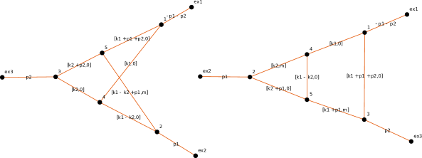
Figure 1: Left: Non-planar vertex with one massive crossed line. Right: Planar vertex with a finite part in the $\epsilon$ expansion represented by the single 3-dimensional MB integral of Eqn. (3). Figures generated by PlanarityTest [22, 24]. Both vertices are special cases for which analytical solutions are available.

In this case, results obtained for the constant parts of the $\epsilon$-expansion with different methods and programs in the Euclidean region are, for $(p_{1}+p_{2})^{2}=-m^{2}=-1$:

$$\begin{array}[]{ll}{\text{ Analytical\; \cite[cite]{[\@@bibref{Number}{Fleischer:1998nb}{}{}]}:}}&-{\color[rgb]{1,0,0}{0.4966198306057021}}\\ {\text{ MB (Vegas)\; \cite[cite]{[\@@bibref{Number}{Czakon:2005rk}{}{}]}:}}&-{\color[rgb]{1,0,0}{0.496}}9417442183914\\ {\text{ MB (Cuhre)\; \cite[cite]{[\@@bibref{Number}{Czakon:2005rk}{}{}]}:}}&-{\color[rgb]{1,0,0}{0.49661983}}13219404\\ {\text{ FIESTA\; \cite[cite]{[\@@bibref{Number}{Smirnov:2015mct}{}{}]}:}}&-{\color[rgb]{1,0,0}{0.496618}}4488196595\\ {\text{ SecDec\; \cite[cite]{[\@@bibref{Number}{Borowka:2017idc}{}{}]}:}}&-{\color[rgb]{1,0,0}{0.49661983}}13167105\end{array}$$ (1)

In the Minkowskian region, with $(p_{1}+p_{2})^{2}=m^{2}=1$:

$$\begin{array}[]{lc}{\text{ Analytical \; \cite[cite]{[\@@bibref{Number}{Fleischer:1998nb}{}{}]}:}}&-{\color[rgb]{1,0,0}{0.778599608979684}}-{\color[rgb]{1,0,0}{4.123512593396311}}\cdot i\\ {\text{ MBnumerics\;\cite[cite]{[\@@bibref{Number}{Dubovyk:2016aqv,Usovitsch:2018shx}{}{}]} }}:&-{\color[rgb]{1,0,0}{0.778599608}}324769-{\color[rgb]{1,0,0}{4.123512}}600516016\cdot i\\ {\rm MB(Cuhre)}:&-{\color[rgb]{1,0,0}{0.7785}}24251263640-{\color[rgb]{1,0,0}{4.123}}498264231095\cdot i\\ {\rm SecDec}:&{\rm big\;error\;{\bf[2016]},{\color[rgb]{1,0,0}{-0.77}}-i\cdot{\color[rgb]{1,0,0}{4.1}}\;{\bf[2017]},-{\color[rgb]{1,0,0}{0.778}}-i\cdot{\color[rgb]{1,0,0}{4.123}}\;{\bf[2019]}}\\ {\rm pySecDec+rescaling}:&-{\color[rgb]{1,0,0}{0.77859}}8-i\cdot{\color[rgb]{1,0,0}{4.123512}}\;{\bf[2020]}\\ \end{array}$$ (2)

The SecDec group discussed this integral in [32]. Using the splitting method the reported result is $-0.77-i\cdot 4.1$. For pySecDec with quasi-Monte Carlo integration (QMC) [36] and using rescaling for $10^{7}$ generated points, the accuracy is much better. Such integral is relatively easy for the MB method, because it includes only one massive propagator. The result for ${\rm MB(Cuhre)}$ has been obtained with the MB.m options: MaxPoints $10^{7}$, AccuracyGoal 8, PrecisionGoal 8. It took about 5 minutes on a moderate laptop.

Another interesting case is the planar scalar integral in Fig. 1, right.

The MB representation for the constant term of this diagram is three-dimensional:

$$I=\frac{1}{(2\pi i)^{3}}\frac{1}{s^{2}}\int\limits_{-i\infty-\frac{47}{37}}^{i\infty-\frac{47}{37}}dz_{1}\int\limits_{-i\infty-\frac{44}{211}}^{i\infty-\frac{44}{211}}dz_{2}\int\limits_{-i\infty-\frac{176}{235}}^{i\infty-\frac{176}{235}}dz_{3}\left(\frac{m^{2}}{-s}\right)^{z_{1}}\Gamma(-1-z_{1})\Gamma(2+z_{1})\Gamma(-1-z_{12})\Gamma(-z_{2})$$

$$\Gamma^{2}(1+z_{12}-z_{3})\Gamma(1+z_{3})\Gamma(-z_{3})\Gamma^{2}(-z_{1}+z_{3})\Gamma(-z_{12}+z_{3})/\Gamma(-z_{1})\Gamma(1-z_{2})\Gamma(1-z_{1}+z_{3}).$$ (3)

The diagram has also an analytical solution [38] which makes it ideal for a non-trivial comparison of different numerical techniques. Numerical results for Eq. 3 are presented in Tab. 3 for $s=m^{2}=1$.

AS	$-1.{\bf 199526183135}$	$+5.{\bf 567365907880}i$
MB	$-1.{\bf 1995261831}68$	$+5.{\bf 567365907}904i$	Cuhre, $10^{7}$, $10^{-8}$
MB	$-1.{\bf 20}4597845834$	$+5.{\bf 567}518701898i$	Vegas, $10^{7}$, $10^{-3}$
MB	$-1.{\bf 1995}16455248$	$+5.{\bf 5673}76681167i$	QMC, $10^{6}$, $10^{-5}$
MB	$-1.{\bf 19952}7580305$	$+5.{\bf 56736}7345229i$	QMC, $10^{7}$, $10^{-6}$

Table 3: Numerical results for Eq. 3 with $s=m^{2}=1$. AS - analytical solution. For details on different MB integration routines and transformations of the infinite integration region used, see [40]. Table taken from there, shortened.

Numerical results obtained for this integral have been discussed recently in [40] with various transformations of variables and various deterministic and Monte Carlo integrators like the CUHRE routine, VEGAS routine [42, 44], QMC. The QMC quasi-MC or VEGAS Monte Carlo methods surpass CUHRE for higher dimensional integrals. The QMC library seems to be especially suitable for the numerical integration of MB integrals in the Minkowskian region. It will be tested in more detail at the 3-loop level. The new Vegas+ package [46] will be also studied.

In summary, there is substantial progress in the numerical treatment of multi-loop Feynman integral calculations with MB and SecDec, approaching now the massive 3-loop diagrams. The techniques presented here can be extended for the computation of massive three-loop electroweak Feynman integrals needed for Z-peak physics. It is also worth mentioning that the differential equations method [48, 50] and the quoted IBP reductions are rapidly developing [52, 54]. They are expected to be very helpful, if not decisive for solving complete sets of integrals, as the third numerical method in the forthcoming three-loop studies. Based on initial work in this direction we see no showstoppers for this specific technical task, and even though much additional work will be needed to assemble them into phenomenological results, this goal also appears within reach in the foreseeable future.

Acknowledgments.

The work of A.F.  is supported in part by the National Science Foundation under grant PHY-1820760. J.U. received funding from the European Research Council (ERC) under the European Union’s Horizon 2020 research and innovation programme under grant agreement no. 647356 (CutLoops). The work is also supported in part by the Polish National Science Centre under grant no. 2017/25/B/ST2/01987 and COST Action CA16201 PARTICLEFACE.