H₂ mass–velocity relationship from 3D numerical
simulations of jet-driven molecular outflows

Abstract

Context. Previous numerical studies have shown that in protostellar outflows, the outflowing gas mass per unit velocity, or mass–velocity distribution $m(v)$, can be well described by a broken power law $\propto v^{-\gamma}$. On the other hand, recent observations of a sample of outflows at various stages of evolution show that the CO intensity–velocity distribution, closely related to $m(v)$, follows an exponential law $\propto\exp(-v/v_{0})$.

Aims. In the present work, we revisit the physical origin of the mass–velocity relationship $m(v)$ in jet-driven protostellar outflows. We investigate the respective contributions of the different regions of the outflow, from the swept-up ambient gas to the jet.

Methods. We performed 3D numerical simulations of a protostellar jet propagating into a molecular cloud using the hydrodynamical code Yguazú-a. The code takes into account the most abundant atomic and ionic species and was modified to include the H₂ gas heating and cooling.

Results. We find that by excluding the jet contribution, $m(v)$ is satisfyingly fitted with a single exponential law, with $v_{0}$ well in the range of observational values. The jet contribution results in additional components in the mass–velocity relationship. This empirical mass–velocity relationship is found to be valid locally in the outflow. The exponent $v_{0}$ is almost constant in time and for a given level of mixing between the ambient medium and the jet material. In general, $v_{0}$ displays only a weak spatial dependence. A simple modeling of the L1157 outflow successfully reproduces the various components of the observed CO intensity–velocity relationship. Our simulations indicate that these components trace the outflow cavity of swept-up gas and the material entrained along the jet, respectively.

Conclusions. The CO intensity–velocity exponential law is naturally explained by the jet-driven outflow model. The entrained material plays an important role in shaping the mass–velocity profile.

1 Introduction

Outflows from young stellar objects (YSOs) can exhibit a great variety of morphological and physical characteristics. In the youngest ($10^{4}\hbox{\kern 1.99997ptyr}$) and deeply embedded Class 0 protostars (André, Ward-Thompson & Barsony, 2000), outflows are easily traced using the CO molecule and their presence is ubiquitous in star forming regions, indicating that they are a common manifestation of both low- and high-mass star formation processes (Wu et al., 2004; Lee, 2020). On the other hand, protostellar jets were first associated with more evolved Class II objects, that is, optically revealed pre-main sequence objects that are still accreting (or classical T-Tauri stars). These jets are observed mainly through forbidden atomic emission lines, like [S II] and [N II], as well in H$\alpha$ (Reipurth & Bally, 2001). In between these two limiting cases, Class I protostars, with a typical age of $10^{5},$ may show evidence for both molecular outflows and protostellar jets at the same time (e.g., L1448 IRS 2 and IRS 3, see Bally, Devine & Alten, 1997). Sometimes a fast and collimated molecular jet is also observed, as in Cep E-mm (Lefloch et al., 2015) or HH 212, which are associated with a Class 0 source (Zinnecker, McCaughrean & Rayner, 1998; Lee et al., 2017).

Nevertheless, the origin of the molecular outflows associated with YSOs is still debated (see Lee, 2020, for a recent review). They are believed to be the by-product of an interaction between a more collimated jet and/or wind, produced in or by the star–disk interaction, and its surrounding medium (Bally, 2016). As the wind and/or jet bow shock propagate into the ambient medium, the gas of the excavated cavity walls advances and excites a profusion of molecular emission lines. For low mass YSOs in particular, this can take place via one of three main mechanisms (see Arce et al., 2007, for a comprehensive review): (i) In wind-driven shell models, a wide-angle wind is supposed to accelerate the ambient medium gas. In this class of models, both the wind and the surrounding medium are assumed to be stratified in density. (ii) In turbulent jet models, a jet subject to dynamical Kelvin-Helmholtz instability can entrain gas through a growing turbulent layer, giving rise to an outflow. This mechanism can also operate at the leading working surface. (iii) In Jet bow-shock models, a collimated jet produces a leading bow shock that accelerates the ambient medium gas. Also, an intermittent jet may develop a set of internal working surfaces that can help in the process (Raga & Cabrit, 1993).

As emphasized in Arce et al. (2007), it is possible that more than one mechanism is operating to produce a given molecular outflow, or alternatively a given mechanism can dominate at different epochs in the evolution of a given source. In any case, a parameter that has been historically used to identify useful models is the slope of a power law that relates the mass of the outflowing molecular gas with its velocity, or $m(v)\propto v^{-\gamma}$. Rigorously speaking, the mass–velocity relationship, sometimes called the mass spectrum, is obtained by considering the mass in a given radial velocity bin, meaning that the observed relationship is actually $\delta m(v)/\delta v\propto v^{-\gamma}$ (see Arce & Goodman, 2001, for a discussion). However, for the sake of simplicity, some authors refer to the mass–velocity relationship as $m(v)\propto v^{-\gamma}$ (Downes & Ray, 1999; Downes & Cabrit, 2003). The mass–velocity relationship gives us the mass of the outflow at a given radial velocity. We note that what is actually observed is the intensity of a given emission line, typically the ¹²CO (1-0) line profile, and that such an intensity correlates with the velocity as described above (Downes & Ray, 1999; Arce & Goodman, 2001). The intensity is then converted to mass (corrected or not by the opacity) to finally obtain the mass–velocity relationship. Molecular outflows seem to display a mass–velocity relationship that can be described by a broken power law (Bachiller & Tafalla 1999; Ridge & Moore 2001; Arce & Goodman 2001), with shallower slopes ($\gamma<2$) at low velocities ($v<10\hbox{\kern 1.99997ptkm\kern 1.99997pts${}^{-1}$}$) and steeper slopes ($\gamma>3$) at intermediate-to-high velocities ($v>10\hbox{\kern 1.99997ptkm\kern 1.99997pts${}^{-1}$}$). In this way, no matter the mechanism used to model a molecular outflow, the model should account for the observed slopes.

In the present paper, we focus on the molecular mass–velocity relationship for molecular outflows produced by a collimated and supersonic jet using three-dimensional numerical simulations. As the jet interacts with the ambient medium, jet-entrained gas and ambient gas swept up by the jet-driven bow-shock can in principle be disentangled. The appeal of such a scenario is two-fold: (i) there is increasing evidence that both phenomena may coexist in Class 0 and Class I sources, as mentioned in the previous paragraph, and (ii) molecular outflows produced by either jet entrainment or a jet-driven bow-shock can effectively end up in a power-law mass–velocity relationship (Chernin & Mason 1993; Zhang & Zheng 1997; Stahler & Palla 2004). In the following section, we briefly compile some previously important results obtained through numerical simulations of jet-driven molecular outflows, and discuss some recent observational findings that ultimately motivated the present work.

2 Previous numerical results and observed intensity–velocity relationships

Numerical simulations of molecular jets have been used extensively in the literature as an efficient tool to investigate the kinematical properties of jet-driven molecular outflows (see Downes & Ray, 1999; Downes & Cabrit, 2003; Rosen & Smith, 2003, 2004a; Smith & Rosen, 2005, 2007). The mass–velocity and intensity–velocity relationships $I_{\rm CO}(v)$ observed in low-J ($\leq 8$) CO lines in molecular outflows have been studied by various authors as a possible test for discriminating between entrainment mechanisms (see Downes & Cabrit, 2003, hereafter, DC03).

Previous works have described the CO intensity–velocity distribution $I_{\rm CO}(v)$ in outflows as a broken power law, $I_{\rm CO}(v)\propto v^{-\gamma}$ with $\gamma\simeq 1.8$ up to line-of-sight velocities $v_{\rm break}\approx$10 – 30 kms^-1 and a steeper slope $\gamma=3$ – 7 at higher velocities (see Frank et al., 2014, for a review). The CO intensity–velocity distribution behavior was successfully reproduced by HD simulation of jet-driven flows, and was found to be the result of CO dissociation above shock speeds of $\sim 20\hbox{\kern 1.99997ptkm\kern 1.99997pts${}^{-1}$}$ and of the temperature dependence of the line emissivity (see DC03).

Downes & Ray (1999) introduced the H₂ molecule in their calculations and found that the H₂ mass–velocity distribution $m(v)\propto v^{-\gamma}$ follows a similar relationship to the intensity–velocity relationship observed in the millimeter rotational lines of CO. Downes & Cabrit (2003) showed that the swept-up molecular gas follows a mass–velocity relationship ($m_{{\rm H}_{2}}(v)$) similar to the intensity–velocity relationship $I_{{\rm H}_{2}}(v)$ in the low velocity range ($v\lesssim 30$ kms^-1). In contrast, in the high velocity range these latter authors found that $I_{{\rm H}_{2}}(v)$ is shallower than $m_{{\rm H}_{2}}(v)$, while $I_{{\rm CO}}(v)$ is steeper than $I_{{\rm H}_{2}}(v)$ but comparable to $m_{{\rm H}_{2}}(v)$.

Rosen & Smith (2003) focused on time-dependent jets, that is, jets whose density varies as a function of time with respect to the ambient medium. These latter authors found that the mass–velocity distribution is systematically shallower than the CO intensity–velocity distribution. They also found that the indices of the distributions are essentially unchanged when considering atomic or molecular jet material.

Keegan & Downes (2005) studied the temporal evolution of the power index $\gamma,$ and their results are consistent with those of Downes & Cabrit (2003). Interestingly, Keegan and Downes found that $\gamma$ should increase slowly in time, attaining a limiting value after $t\approx 1500$ years.

We note that simulations and observational work have focused on the global properties (mass, etc.) and not on local properties inside the outflows. Also, the underlying bow-shock model predicts a power law at low velocities on long computational timescales much longer than the dynamical timescales derived from observations, which are usually a few thousand years (see also Rosen & Smith, 2003, 2004a; Smith & Rosen, 2005, 2007).

The discovery that the CO line profiles observed towards the protostellar outflow L1157 could be very well fitted by an exponential law $I_{\rm CO}(v)\propto\exp(-v/v_{0})$, with $v_{0}\sim 2-12\hbox{\kern 1.99997ptkm\kern 1.99997pts${}^{-1}$}$, came as a surprise (Lefloch et al., 2012). Further observational studies confirmed that these spectral signatures, with similar values of $v_{0}$, were detected in a plethora of molecular gas tracers, like CS (Gómez-Ruiz et al., 2015), HNCO and NH₂CHO (Mendoza et al., 2014), HC₃N (Mendoza et al., 2018), and HCO⁺ (Podio et al., 2014).

The same analysis applied to the outflow sample of Bachiller & Tafalla (1999) observed in the CO $J$=2–1 line (L1448, Orion A, NGC2071, L1551 and Mon R2) yielded a similar conclusion. The sample contains sources at various stages of evolution from early Class 0 (e.g. L1448) to late Class I (e.g. L1551). Lefloch et al. (2012) showed that all the sources could be fitted by a single exponential $I_{\rm CO}(v)\propto\exp(-v/v_{0})$, with values of $v_{0}$ between 2 and $12\hbox{\kern 1.99997ptkm\kern 1.99997pts${}^{-1}$}$, well in the range of those determined in L1157-B1. Also, Lefloch et al. observed the trend that the more evolved, Class I outflows of the sample (Mon R2, L1551) display a shallower intensity–velocity distribution. Therefore, an exponential relation $I_{\rm CO}(v)\propto\exp(-v/v_{0})$ is found to be a good approximation of the observed intensity relation not only in L1157-B1 but in several molecular outflows in general, with a reduced number of free parameters compared to a broken power law. Mapping of the CO $J=$ 3–2 emission over the L1157 outflow by Lefloch et al. (2012) showed that the exponential spectral signature is detected along the outflow cavity walls in the southern outflow lobe, implying that it is not only a global, but also a local signature of the outflowing gas.

In summary, molecular outflowing gas shows an intensity–velocity relationship well described by an exponential power law, both on a global and local scale. The question arises as to how this general property of molecular outflows is related with the outflow mechanism itself. In order to address this question, we carried out three-dimensional (3D) hydrodynamics (HD) simulations of the evolution of ouflowing gas in a dense medium representing the parental molecular cloud/surrounding protostar envelope. Specifically, we present a new methodology based on distinguishing the mixing level between the ambient medium and the jet gas, which helped us to disentangle the distinct components that arise in the H₂ mass–velocity relationship. The article is organized as follows. In §3.1 and §3.2 we provide details of the numerical setup and initial parameters for the simulations. In §3.4 we briefly compare our results with some previous numerical studies of molecular jets. In §4 and 5 we present the results of our numerical simulations and we discuss their implications for observations of molecular outflows using L1157 as a reference. In §6 we present our conclusions.

3 Numerical simulations

3.1 Numerical setup

The simulations presented here were performed using the Yguazú-a code (Raga, Navarro-González & Villagrán-Muniz, 2000; Raga et al., 2002; Cerqueira et al., 2006). In its original version, the code was designed to solve hydrodynamic problems with a chemical network for the following atomic and ionic species: HI, HII, HeI, HeII, HeIII, CII, CIII, CIV, NI, NII, NIII, OI, OII, OIII, OIV, SII and SIII. For the present work, we introduced the H₂ molecule as a new species and added three dissociation reactions for molecular hydrogen:

$$\rm H+H_{2}\rightarrow 3H\,{\rm,}$$ (1)

$$\rm H_{2}+H_{2}\rightarrow 2H+H_{2}\,{\rm,}$$ (2)

$$\rm e+H_{2}\rightarrow e+2H\,{\rm.}$$ (3)

We used the collisional dissociation rates of molecular hydrogen provided in Shapiro & Kang (1987) for these three reactions. We also calculated the cooling function considering both the radiative and the dissociative processes. For the radiative cooling rate, we used the fit proposed by Lepp & Shull (1983), which considers both the rotational and vibrational cooling from the two reactions, H-H₂ and H₂-H₂ , in both high- and low-density regimes ($n<n_{cr}\approx 10^{4}$ cm^-3). The dissociative cooling function was taken from Shapiro & Kang (1987). In Fig.  1 we show the different cooling functions: atomic (blue line) and molecular dissociative (green line) and radiative cooling (red line) .

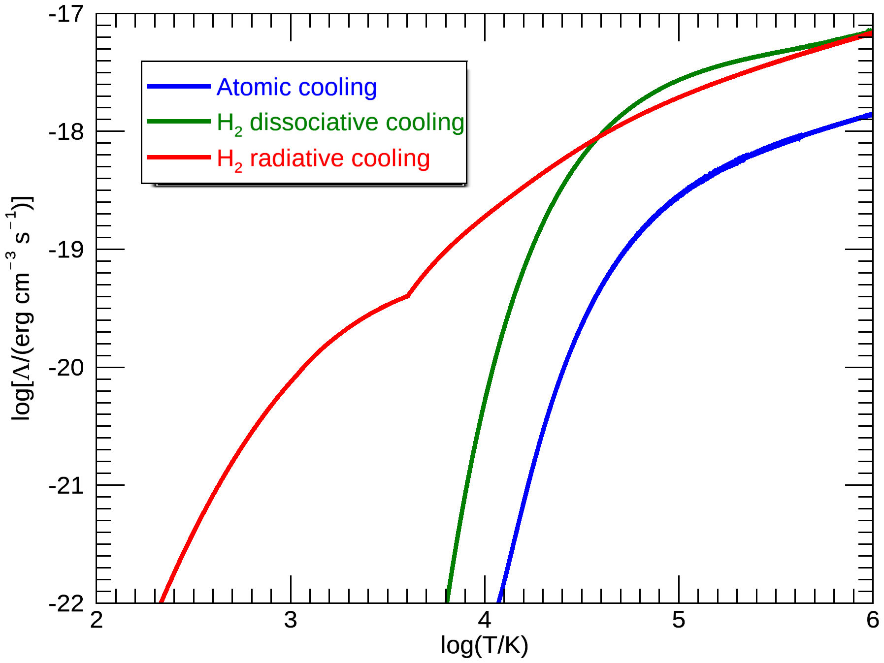
Figure 1: Different contributions for the cooling: atomic emission lines (blue line), H₂ dissociative cooling (green line), and H₂ radiative cooling (red line). The cooling functions were calculated using the starting values (i.e., at $t=0$) for the numerical densities, or $n_{{\rm HI}}$ = 8.31 cm^-3, $n_{{\rm HII}}=0.08$ cm^-3, $n_{{\rm He}}=15.94$ cm^-3 and $n_{{\rm H}_{2}}=75.51$ cm^-3.

Table 1: Jet models

Model	$v_{j,0}$	A	$n_{a}$	$n_{j}$	$\eta$	$T_{a}$	$T_{j}$	$\tau_{P}$	$\theta$	$N_{tot}$	$\tau_{e}$
	(km s-1)		(cm-3)	(cm-3)		(K)	(K)	(years)	(∘)		(years)
DR_SS	212	0	100	100	1	100	1000	-	-	-	-
DR	212	0.15	100	100	1	100	1000	-	-	4	5, 10, 20 and 50
DR_P	212	0.15	100	100	1	100	1000	200	6	4	5, 10, 20 and 50

Together with H₂, CO and H₂O have long been known to play an important role in shocked gas cooling (Hollenbach & McKee, 1979; Kaufman & Neufeld, 1996; Flower & Pineau des Forêts, 2010). Detailed observational studies have confirmed that line cooling from CO and H₂O can be as important as that from H₂ in protostellar outflows (see e.g. Nisini et al., 2010a; Busquet et al., 2014). Modeling of the structure of outflow shocks may be significantly modified by the inclusion of additional terms such as CO, H₂O, or even charged grains (see e.g. Flower & Pineau des Forêts, 2010), all of which are not taken into account here. In the present work, we have not included either the H₂O or the CO chemical networks or their related cooling terms. This would represent an effort which is well beyond the state of the art of 2D and 3D chemo-hydrodynamical codes such as WALKIMYA-2D (Castellanos-Ramírez et al., 2018, Rivera-Ortiz et al., in prep.). However, we note that Rosen & Smith (2004a) included equilibrium C and O chemistry in their numerical scheme in order to calculate the CO, OH, and H₂O abundances, as well as to estimate the cooling expected from these molecules. They concluded that the mass–velocity relationship is always shallower than the intensity–velocity relationship, confirming previous results based only on H₂ (Downes & Cabrit, 2003) . For that reason, the present work focuses on the entrained gas properties and we aim to revisit the H₂ mass–velocity relationships, whose properties can be accessed following the present prescription.

Our computational domain is a Cartesian 3D rectangular box with the following dimensions:

$$(x,y,z)=(2,\leavevmode\nobreak\ 2,\leavevmode\nobreak\ 8)\times 10^{4}\leavevmode\nobreak\ {\rm au}\,,$$ (4)

and the jet propagates along the $z-$ direction.

The Yguazú-a is a multi-level binary adaptive grid code. Here we use a five-level grid which has ($x$, $y$, $z$) = (256, 256, 1024) cells in its high-resolution mode. This gives a maximum resolution of $\Delta x=\Delta y=\Delta z=78.13$ au. The jet radius is initially always given by $R_{j}=391$ au or $\sim 5\Delta x$. The jet radius is therefore compatible with those adopted in previous numerical simulations (Downes & Ray, 1999; Downes & Cabrit, 2003) as well as with estimates for the HH jet radius (Reipurth et al., 2000, 2002; Podio et al., 2006).

3.2 Physical conditions

Three cases were considered, which are summarized in Table 2:

• model DR: an intermittent jet model for comparison with previously published simulations in the literature (DC03, Downes & Ray 1999);

• model DR_SS: a steady state jet;

• model DR_P: an intermittent, precessing jet model.

With model DR_P, we aim to investigate the properties of the L1157 outflow, kinematical studies of which have revealed convincing evidence of precession (Gueth, Guilloteau & Bachiller, 1996; Podio et al., 2016). In this simulation (and for model DR) we assume that the jet velocity varies periodically with time, according to:

$$v_{j}=v_{j,0}\cdot\bigg{[}1+A\sum_{i=1}^{N_{tot}}{\rm sin}\bigg{(}\frac{2\pi}{\tau_{e,i}}\cdot t\bigg{)}\bigg{]}\,,$$ (5)

where $v_{j,0}$ is the jet velocity, $A=\Delta v/v_{j,0}$ is the adopted amplitude variation for the jet velocity variation, and $\tau_{e}$ is the variability period ($t$ is the time). In our time-varying models, $N_{tot}=1$ or 4, and $5\lesssim\tau_{e,i}\lesssim 50$ years (see Table 2). We note that although Eq. 5 has been used here in an attempt to reproduce the model presented in DC03, the idea that Herbig-Haro objects can be generically explained by successive internal knots promoted by a sinusoidal jet velocity variability is well established (e.g., Reipurth & Bally, 2001). However, a detailed source modeling can require a superposition of different sinusoidal terms, which have been discussed by Castellanos-Ramírez, Raga & Rodríguez-González (2018; see also Bally 2016), indicating that a multimode jet velocity variability may be important to explain the observed morphology and kinematics in some sources. For the precessing case DR_P, we adopted a precessing angle of $\theta=6^{\circ}$ and a precessing period of $\tau_{P}=200$ years. The DR model has the same parameters as the model presented in DC03.

In all models, we assume solar elemental abundances for both ambient and jet material. The ratio $n_{{\rm H}_{2}}/n_{\rm H}=9$ (here and after, $n_{\rm H}=n_{\rm HI}+n_{\rm HII}$) is initially imposed for both the jet and the ambient medium (Downes & Ray, 1999; Nisini et al., 2010b). The helium fraction per hydrogen nuclei is assumed to be $n_{\rm He}/[n_{\rm H}+2n_{{\rm H}_{2}}]=0.1$ With these choices, the equation of state is calculated for a gas with a mean molecular weight of $\mu=2.23$ and $C_{V}=2.25$. The ionization fraction of hydrogen in the jet is initially taken as $f_{H}=0.01$ for $T_{j}=10^{3}$ K in agreement with the values inferred from atomic line observations of HH jets in the optical (Podio et al., 2006).

The ambient medium and jet parameters such as numerical density $n$, temperature $T$, and jet velocity are all given in Table 2, along with the jet precessional and intermittence periods of the simulated models.

Observationally, the jet temperature and density determinations span a wide range of values depending on the tracer used. Optical atomic line observations yield $T_{j}\sim 5\times 10^{3}-2\times 10^{4}$ K (Podio et al., 2006) while molecular line observations indicate lower values of about $10^{3}-3\times 10^{3}$ K from near-infrared H₂ rovibrational transitions (e.g., Caratti o Garatti et al., 2006), and $T_{j}\sim$ 100-500 K from (submillimeter) CO and SiO rotational lines (Nisini et al., 2007; Lefloch et al., 2015). In the optical, inferred jet densities have values of $n_{j}\sim 10^{3}-10^{4}\hbox{\kern 1.99997ptcm${}^{-3}$}$ , while (sub)millimeter line observations yield high values, $n_{j}\gtrsim 10^{5}$ cm^-3. This wide range of physical conditions reflects the intrinsic complexity of the jet, which is often associated with internal shocks that drive the formation of strong temperature and density gradients. Adopting single initial values for temperature and density is most likely an oversimplified description of the jet physical structure. We note however that the initial jet temperature value adopted in the simulations are consistent with those obtained from jet molecular line observations (H₂, SiO, CO). The initial jet density in our simulations is $100\hbox{\kern 1.99997ptcm${}^{-3}$}$ (same as in DC03), which is lower than the values determined observationally. However, it is the jet-to-ambient density ratio which carries the most weight in modeling the dynamical evolution of the outflow. This point was investigated in detail by Rosen & Smith (2004b). Based on their results, we do not expect significant differences in the simulations when adopting a higher density for the jet, provided that the jet-to-ambient density ratio is kept constant.

3.3 Mass–velocity profiles

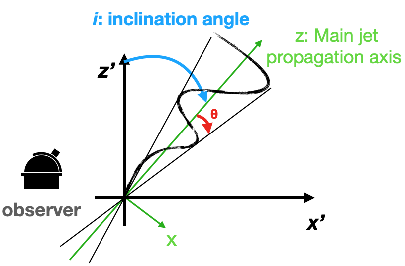
Figure 2: Sketch of the geometry of the flow with respect to the observer. The jet propagates along the $z$-axis, which is inclined by an angle $i$ with respect to the plane of the sky ($y^{\prime}-z^{\prime}$). In case of precession, the jet draws a cone with a half angle of $\theta$ with respect to the $z$-axis.

Our primary diagnostics are the mass–velocity relationship for both the total mass $m(v)$ and the molecular mass, $m_{{\rm H}_{2}}(v)$, which are computed for the whole computational domain or for a given spatial region. In order to obtain the mass–velocity profiles, we first compute the column density $N$ as the sum of particle density along the line of sight per velocity interval:

$$N(y^{\prime},z^{\prime})\bigg{|}_{v=v_{\rm CM}}=\sum n^{\prime}\Delta x^{\prime}\leavevmode\nobreak\ \,,$$ (6)

where

$$v=v_{x}{\rm cos}i-v_{z}{\rm sin}i\leavevmode\nobreak\ .$$ (7)

In Equation (6), $\Delta x^{\prime}$ is the projection of the $x-$coordinate along the line of sight and $n^{\prime}$ is the numerical particle density (total or molecular) in the radial velocity range $(v-\Delta v/2)<v<(v+\Delta v/2)$, where we set $\Delta v=1\hbox{\kern 1.99997ptkm\kern 1.99997pts${}^{-1}$}$. In Equation (7), $i$ is the inclination angle with respect to the plane of the sky (see Fig. 2), meaning that $v$ corresponds to the (observed) radial velocity.

As the jet propagates, interaction with the ambient gas leads to the formation of a mixed gas layer from jet and ambient material. In order to estimate the relative contribution of the different regions of the outflow, namely the swept-up ambient medium and the mixed (jet plus ambient medium) material, we tagged the jet material with a passive scalar or tracer $j$. This passive scalar is set to $j=0$ in the ambient medium and to $j=1$ in the jet, and is advected by the flow. As the jet interacts with the ambient medium and mixing occurs, the local value of the scalar represents the relative fraction of initially jet material within a given cell. With this we introduce a parameter $j_{mix}$ to indicate the level of mixing considered, such that $j\leq j_{mix}$. Thus, material with $j_{mix}=0$ would correspond to ambient unmixed medium, that with $j_{mix}=0.5$ would include material that has a jet fraction up to $0.5$, and that with $j_{mix}=1$ will include all jet and ambient material.

3.4 Comparison with previous work

We tested our numerical scheme against previous numerical simulations published in the literature by running model DR (Table 2). The parameters of model DR were chosen to mimic model G in Downes & Ray (1999), as well as the “pulsed” model discussed in Downes & Cabrit (2003).

Briefly, the DR model has jet ($n_{j}$) and ambient medium ($n_{a}$) numerical particle density $n_{j}=n_{a}=100$ cm^-3, jet temperature $T_{j}=1000$ K, ambient medium temperature $T_{a}=100$ K, molecular hydrogen to hydrogen numerical density ratio $n_{{\rm H}_{2}}/n_{{\rm H}}=9,$ and a helium to hydrogen numerical density ratio of $n_{{\rm He}}/n_{\rm H}=0.1$. The only H₂ dissociation process considered in this model is collisions with H atoms, and the rate coefficient used here is given by:

$$k_{D,H-H_{2}}=2\times 10^{-10}{\rm exp}(-55\,000/T)\leavevmode\nobreak\ \leavevmode\nobreak\ {\rm cm}^{3}{\rm s}^{-1}\leavevmode\nobreak\ \,,$$ (8)

following Taylor & Raga (1995).

Figure 3 shows the results of model DR at $t$= $400\hbox{\kern 1.99997ptyr}$. Depicted in this figure are the midplane ($x=0$) distribution of the tracer (panel $a$), the temperature (panel $b$), the velocity components along the $z-$axis (panel $c$) and the $y-$axis (panel $d$), the total particle density $n$ (panel $e$), and the molecular particle density $n_{{\rm H}_{2}}$ (panel $f$). We plot a white contour line that separates the original (quiescent and/or disturbed) ambient medium where the tracer $j_{mix}$ is zero (the region outside the contour line) from the inner jet where $j_{mix}=1$ (see Fig. 3).

Figures 3($e)$ and 3$(f)$ show the internal working surfaces at $z$= 2500, 5000, and 7500 au, where both the total density and the molecular density increase. The leading bow shock is more pronounced in the density maps (panels $e$ and $f$). Although density enhancement is observed in the internal shocks (see Fig. 3) as expected, neither the total density nor the molecular density attain their maximum values at the internal working surfaces. The region where the total density is maximum is located at the head of the jet and inside the contour line, indicating that the jet and the ambient medium have already been mixed. It is important to note that while the molecular density is higher at the $external$ edges of the laterally expanding trails of the leading bow shock, the total density peaks are near to the jet axis and the apex of the leading bow shock. This occurs because strong shocks at the jet head dissociate the molecular hydrogen, while the shocks are weaker at the bow shock trails and the molecular hydrogen piles up without being dissociated. We already anticipate that the mass–velocity profiles extracted from our simulations should present a high-velocity component ($v\sim 100\hbox{\kern 1.99997ptkm\kern 1.99997pts${}^{-1}$}$) if some mixing between the jet and the ambient medium material is allowed.

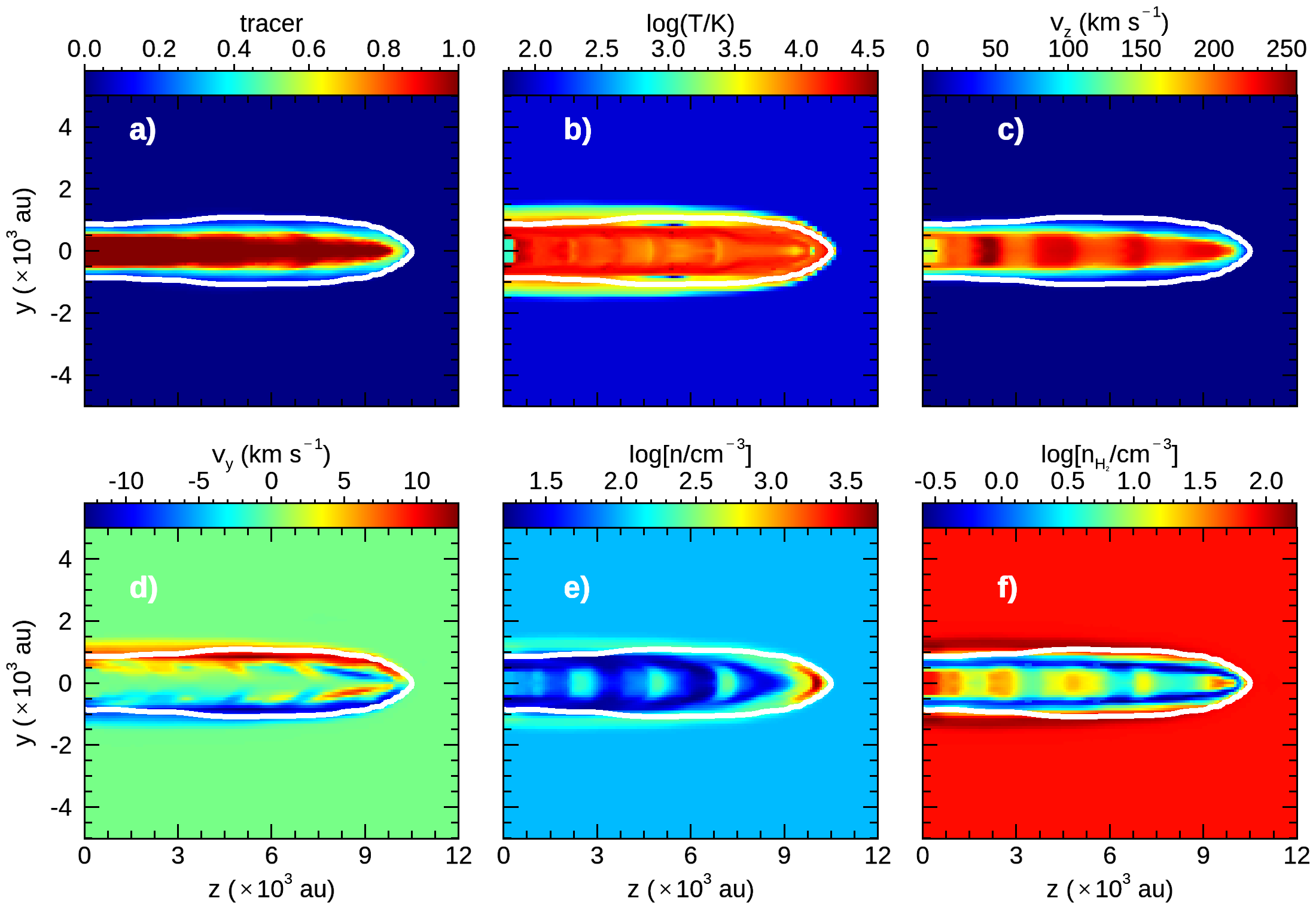
Figure 3: Model DR at $t$= $400\hbox{\kern 1.99997ptyr}$. Distributions in the plane $x$=0 of $(a)$ $j_{mix}$ (tracer), $(b)$ temperature, $(c)$ $v_{z}$, $(d)$ $v_{y}$, $(e)$ total density $n,$ and ($f)$ molecular gas density $n_{{\rm H}_{2}}$. The white line in each panel separates the region in the computational system filled by the ambient medium —where the tracer is equal to zero— from the mixing region and the jet itself.

3.4.1 Comparison with Downes and Ray (1999)

In this section, we compare the results of model DR (see Table 2) with the results of Downes & Ray (1999). More precisely, we compare the results of the mass–velocity distribution at $t$= $300\hbox{\kern 1.99997ptyr}$ and for an inclination angle of $i=60^{\circ}$ with respect to the observer for a direct comparison with Fig. 3 in Downes & Ray (1999). In Fig. 4 we report the molecular mass–velocity profile obtained when integrating over a region defined by a minimum level of mixing between the jet and ambient medium material from $j_{mix}$= 0 (ambient only; top panel) to $j_{mix}=1.0$ (from ambient plus jet; bottom panel). We have superposed the best fit obtained using a power-law $m(v)\propto v^{-\gamma}$ in red. For the sake of clarity, we have made adjustments for two distinct radial-velocity intervals: $0<v<10$ km s^-1 and $10<v<100$ km s^-1. Hereafter, $v$ is used to refer to the radial velocity.

The mass–velocity relations in Fig. 4 are well described by a broken power law. At $v\sim 10\hbox{\kern 1.99997ptkm\kern 1.99997pts${}^{-1}$}$, the slope changes in all cases from $j_{mix}=0$ up to $j_{mix}=1.0$. As expected, the slope in the low-velocity range is always shallower than in the high-velocity range. However, there is an important and systematic effect in the slopes caused by the jet material removal from the integration process that results in an overall steepening in the mass–velocity relation.

We can see in Fig. 4 that considering different levels of jet content in the computation of the mass–velocity relation induces a similar effect: in the high-velocity range ($v>10$ km s^-1), the slopes are steeper for lower values of $j_{mix}$. By contrast, in the low-velocity range ($v\leq 10\leavevmode\nobreak\ \hbox{\kern 1.99997ptkm\kern 1.99997pts${}^{-1}$}$) the slopes barely vary with $j_{mix}$. We interpret these facts as a consequence of effect of mass addition in a given velocity channel, when we go deeper into the mixing layer. In the low-velocity range the profile is dominated by the material of ambient origin, which can be either swept-up gas by the jet-driven bow-shock or entrained gas that barely interacted with the jet. The contribution of the jet and/or ambient interacting material becomes increasingly apparent when considering increasing $j_{mix}$ values in the high-velocity range.

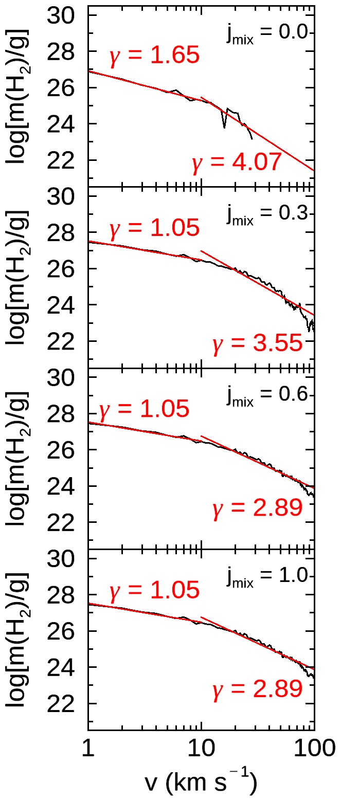
Figure 4: Model DR at $t=300\hbox{\kern 1.99997ptyr}$ and an inclination angle of $i=60^{\circ}$. Molecular mass–velocity relationship $m_{{\rm H}_{2}}(v)$ (black) for the $0\hbox{\kern 1.99997ptkm\kern 1.99997pts${}^{-1}$}<v<100\hbox{\kern 1.99997ptkm\kern 1.99997pts${}^{-1}$}$ radial velocity range and the best-fitting power law $m(v)\propto v^{-\gamma}$ (red). The best-fitting index value $\gamma$ is shown inside each panel for two intervals: $0\hbox{\kern 1.99997ptkm\kern 1.99997pts${}^{-1}$}<v<10\hbox{\kern 1.99997ptkm\kern 1.99997pts${}^{-1}$}$ (left) and $10\hbox{\kern 1.99997ptkm\kern 1.99997pts${}^{-1}$}<v<100\hbox{\kern 1.99997ptkm\kern 1.99997pts${}^{-1}$}$ (right). The $j_{mix}$ parameter is also indicated (from top to bottom, $j_{mix}=$ 0, 0.3, 0.6 and 1.0). The vertical axis displays the logarithm of the molecular mass (in g).

In their simulation run, Downes & Ray (1999) obtained a mass–velocity distribution which was best fitted with a power law of index $\gamma=2.98$ in the range $10<v<100$ km s^-1 (see their Fig. 3). In our simulation run with the same set of parameters with Yguazú-a, we obtain a similar mass–velocity relationship, which can be fitted by a power law (Fig. 4). However, we find that the power-law index depends on the degree of mixing between the jet and the entrained ambient material, i.e., with the value of $j_{mix}$. For the swept-up (unmixed) molecular material ($j_{mix}=0$), the mass–velocity relationship is best fitted by a power law of index $\gamma=4.07$, which is steeper than the value found by Downes & Ray (1999). However, if we take into account the contribution of mixed ambient and jet material (e.g., $j_{mix}=0.6$) to the mass–velocity relationship, we obtain a best fit with a power law with a shallower index of $\gamma$= 2.89, which is very close to that found by Downes & Ray (1999). This results also holds when we take into account all the material along the line of sight while assuming full mixing between the jet and the ambient material ($j_{mix}=1.0$).

We conclude that our simulations are in very good agreement with those of Downes & Ray (1999). We can retrieve their results with excellent accuracy in the limit of large mixing degree ($j_{mix}\geq 0.6$). Our results suggest that the jet contribution must also be taken into account when studying the mass–velocity distribution.

3.4.2 Comparison with Downes and Cabrit (2003)

Using a numerical code very similar to that of Downes & Ray (1999) and with similar initial conditions, DC03 further investigated the mass–velocity and intensity–velocity relations in the CO J=2–1 and H₂ S(1) v=1–0 lines for jet-driven molecular outflows.

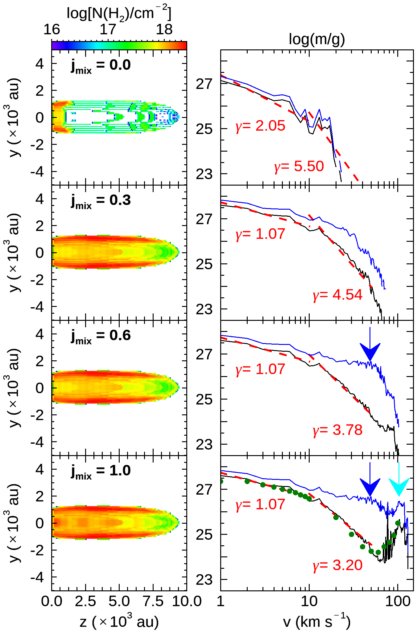
Figure 5: Model DR at $t=400$ yr and an inclination angle $i$= $30^{\circ}$. The results are presented for four different values of the jet and ambient gas mixing degree $j_{mix}$ (from top to bottom): 0.0, 0.3, 0.6, 1.0. (left) Maps of H₂ column density obtained by integration over the velocity range, between $+1$ and $+150\hbox{\kern 1.99997ptkm\kern 1.99997pts${}^{-1}$}$. (right) Mass–velocity relationship obtained for the molecular gas (black) and the total gas (blue). In the bottom panel ($j_{mix}=1.0$), the green dots correspond to the H₂ swept-up mass–velocity relationship obtained by DC03 (see their Fig. 2). We show the best-fitting power laws $m(v)\propto v^{-\gamma}$ to the velocity intervals $v\leq 10\hbox{\kern 1.99997ptkm\kern 1.99997pts${}^{-1}$}$ and $10<v\lesssim 20\hbox{\kern 1.99997ptkm\kern 1.99997pts${}^{-1}$}$ superposed in red dashed lines. The power-law index $\gamma$ is given in each panel. The vertical arrows indicate the position of bumps in the total mass–velocity profile (see text).

In Fig. 5 we show maps of H₂ molecular column density (left panels) and the mass–velocity relationships (right panels): the molecular $m_{{\rm H}_{2}}(v)$ (black lines) and the total mass–velocity relations $m(v)$ (blue lines). For the sake of direct comparison with the results presented by DC03 (see their Fig. 2), the molecular mass $m_{{\rm H}_{2}}(v)$ and mass $m(v)$ velocity relationships have been extracted from the DR model at $t=400$ yr, considering an inclination angle of $i=30^{\circ}$ and different values of the jet and ambient gas mixing ratio $j_{mix}$= 0, 0.3, 0.6, 1.0. In order to obtain the molecular mass distribution of the outflow–jet system, we integrated over the full range of velocity, between $+0$ and $+150\hbox{\kern 1.99997ptkm\kern 1.99997pts${}^{-1}$}$, and excluding the emission of the quiescent gas at rest velocity ($v$=0). By doing so, the contrast of the image is enhanced, easily revealing the geometry of the cavity and the presence of the internal working surfaces produced by the jet.

Comparison of the mass–velocity relationships obtained for different values of $j_{mix}$ in Fig. 5 with respect to the swept-up gas (top panel) shows the presence of gas accelerated at $v>10\hbox{\kern 1.99997ptkm\kern 1.99997pts${}^{-1}$}$ already for $j_{mix}=0.3$ and $j_{mix}=0.6$, which results in a shallower mass–velocity distribution. This change of slope is mainly caused by the contribution of the massive gas clump that develops near the apex of the bow shock inside the mixing layer. This effect can be seen in Fig. 3(e).

The total and molecular mass–velocity relationships are very close to each other in the swept-up gas (top panel in Fig. 5), which implies that the molecular gas dissociation can be neglected in the local gas acceleration (entrainment) process. When taking into account the jet–ambient gas mixing, the slope of the total mass–velocity relationship (blue in Fig. 5) starts to depart from the molecular mass–velocity slope (black) for $j_{mix}=0.3$ case. The difference increases with increasing velocity and increasing $j_{mix}$ (jet-ambient mixing ratio) values. The change of slope between $j_{mix}$=0.3 and $j_{mix}$= 0.6 occurs near $v\sim 50\hbox{\kern 1.99997ptkm\kern 1.99997pts${}^{-1}$}$. We note that this velocity coincides with the projected velocity of the high-density gas concentrated at the jet head. This region can be seen in Fig. 3 (e) near $z=9.5\times 10^{3}$ au. The velocity component of this dense component along the jet axis is $v_{z}\approx 100\hbox{\kern 1.99997ptkm\kern 1.99997pts${}^{-1}$}$, which corresponds to a projected (radial) velocity of $50\hbox{\kern 1.99997ptkm\kern 1.99997pts${}^{-1}$}$. The increase of the mass at high velocities (in blue in Fig. 5) with increasing $j_{mix}$ values is essentially unnoticed in the molecular mass–velocity distribution (in black in Fig. 5). This is consistent with efficient H₂ dissociation in the shocks at the jet head.

In the case of full jet–ambient gas mixing ($j_{mix}=1$), a second bump is detected in the mass–velocity distribution at $v\approx 100\hbox{\kern 1.99997ptkm\kern 1.99997pts${}^{-1}$}$ (Fig. 5), which is the signature of the internal knots formed as a result of jet variability. This second bump is present in both the molecular (black lines) and the total mass (blue line) velocity distributions. Again, this is illustrated in Fig. 3, where both total and molecular densities appear to be enhanced behind internal shocks at a velocity consistent with the projected velocities of the second bump. We emphasize that this second bump can only be seen if we consider the total jet material in the calculation ($j_{mix}=1.0$), while the first bump starts to appear at moderate values of $j_{mix}$.

In the bottom right panel of Fig. 5 we have superimposed the results of the Downes & Cabrit (2003) simulation with green bullets. As we can see, the match between the swept-up H₂ –velocity distribution of these latter authors and the results of our simulations is very close. However, it should be noted that DC03 claimed to have obtained the molecular mass–velocity relation for the swept-up H₂, hence excluding the jet material from the computation (see their Fig. 2) . While DC03 claim that the jet has not been considered in their computation of the mass, we were only able to reproduce their profile when taking into account the jet contribution in the computation. The presence of a high-velocity bump in the H₂ mass–velocity distribution is evidence that the jet has been considered in the integration procedure, as discussed above.

To summarize, we carried out a detailed comparison of the Yguazu-a code results with numerical simulations presented by Downes and Ray (1999) and DC03. We obtained excellent quantitative agreement in both cases. This bolsters our confidence in the use of this approach and in the results for the mass–velocity distributions produced by our code.

4 Results

4.1 Steady state

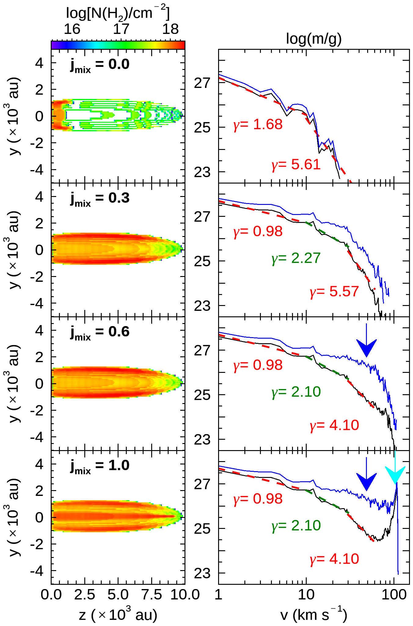
Figure 6: Model DR_SS at $t=400$ yr and an inclination angle $i$= $30^{\circ}$. The results are presented for four different values of the jet–ambient gas mixing degree $j_{mix}$ (from top to bottom): 0.0, 0.3, 0.6, 1.0. (left) Maps of H₂ column density obtained by integration over the velocity range between 1 and $+150\hbox{\kern 1.99997ptkm\kern 1.99997pts${}^{-1}$}$. (right) Mass–velocity relationship obtained for the molecular gas (black) and the total gas (blue). The best-fitting power laws for the three velocity intervals: $v\leq 10\hbox{\kern 1.99997ptkm\kern 1.99997pts${}^{-1}$}$ (left; dashed red), 10 km s^-1 $<v<$ 30 km s^-1 (middle; dashed green) and 30 km s^-1 $<v<$ 60 km s^-1 (right; dashed red) are drawn. The index $\gamma$ for each one of these intervals are shown inside each panel. The vertical arrows indicate the position of bumps in the total mass–velocity profile (see text).

We first present the results of model DR_SS, which simulates the propagation of a nonprecessing jet under steady-state (SS) conditions. The parameters of the simulation are summarized in Table 2. Figure 6 shows the H₂ column density spatial distribution, and the total and molecular mass–velocity distributions obtained for different values of the jet-ambient gas mixing ratio $j_{mix}$= 0, 0.3, 0.6, and 1.0 at $t=400$ yr and for an inclination angle of $i=30^{\circ}$.

The main difference between model DR_SS and the simulation discussed above in Sect. 3 lies in the SS assumption, that is, the absence of intermittency in the mass-ejection process. Many similarities are therefore observed when comparing the mass–velocity relationships obtained in both simulations at a common age of 400 yr, which are presented in Figs. 5-6. The main similarities can be summarized as follows:

• The total mass and the molecular mass–velocity relations associated with the swept-up gas ($j_{mix}=0$) are very similar, and are separated by only a small and constant vertical offset over the whole velocity range ($\lesssim 20\hbox{\kern 1.99997ptkm\kern 1.99997pts${}^{-1}$}$).

• The gap between the total mass and the molecular mass becomes more evident with increasing values of $j_{mix}$ and increasing velocity. For the case $j_{mix}=0.3$, the curves end up at $v\simeq 90\hbox{\kern 1.99997ptkm\kern 1.99997pts${}^{-1}$}$ showing a difference in mass (total versus molecular) of about two orders of magnitude.

• In the $j_{mix}=0.6$ case, a bump is detected in the total mass–velocity relationship at $v\simeq 50\hbox{\kern 1.99997ptkm\kern 1.99997pts${}^{-1}$}$. The lack of detection in the molecular mass–velocity distribution suggests it is mostly of atomic origin and that it traces the signature of material locally accumulated behind the jet head as a result of shock compression.

• A second bump of mainly atomic jet material is detected at high velocity, namely $v\sim 100\hbox{\kern 1.99997ptkm\kern 1.99997pts${}^{-1}$}$ (see panel $j_{mix}=1.0$ in Figs. 5-6).

We therefore conclude that the internal knots that form as a result of the intermittency of the mass-ejection process do not fundamentally alter the mass–velocity relationship obtained in a continuous SS ejection process. However, some differences are seen between the two simulations when comparing the relative contributions of the molecular and atomic material.

The high-velocity bump detected at about $100\hbox{\kern 1.99997ptkm\kern 1.99997pts${}^{-1}$}$ is related to the internal knots in the case of DR, whereas it traces the jet material in the SS model. Though mainly atomic, the bump contains a significant fraction of molecular material. The gap between the total (atomic+molecular) and the molecular mass is wider in the case of intermittent ejection (model DR; Fig. 5) than in the SS regime (Fig. 6). Indeed, H₂ dissociation is expected to occur in the multiple internal shock knots produced in the pulsating model; by comparison, in the SS model, only the leading bow shock is expected to dissociate H₂. This is also well illustrated by panels (e) and (f) in Fig. 3.

The second bump detected at $v\sim 100\hbox{\kern 1.99997ptkm\kern 1.99997pts${}^{-1}$}$ in the DR model (see Fig. 5) is fully developed. This indicates that the jet material reaches a higher velocity in the SS regime, $\geq 100\hbox{\kern 1.99997ptkm\kern 1.99997pts${}^{-1}$}$. As can be seen in Fig 6, in the SS regime, the jet reaches a velocity close to the maximum expected value, $v=212\cdot{\rm sin}30^{\circ}=106\hbox{\kern 1.99997ptkm\kern 1.99997pts${}^{-1}$}$. On the contrary, in a pulsating jet, the formation of internal shocks results in a deceleration of the jet material all along its axis.

We determined the best-fitting power law to the molecular mass–velocity relationship for model DR_SS in the three velocity intervals: $v<10$ km s^-1, 10 $\hbox{\kern 1.99997ptkm\kern 1.99997pts${}^{-1}$}<v<30\hbox{\kern 1.99997ptkm\kern 1.99997pts${}^{-1}$}$ and 30 km s^-1 $<v<$ 60 km s^-1. The results are reported in Fig. 6, where we show the results of model DR_SS at $t=400\hbox{\kern 1.99997ptyr}$ under an inclination $i=30^{\circ}$ with respect to the plane of the sky (see Fig. 2). The slopes of the molecular mass–velocity relationship decrease as $j_{mix}$ increases. In the low-velocity range, the behavior of the relationship is very similar to that obtained for a pulsating jet (model DR; Fig. 5). However, for the $v>10\hbox{\kern 1.99997ptkm\kern 1.99997pts${}^{-1}$}$ and $j_{mix}\geq 0.3$, there is a region at intermediate radial velocities (10 kms^-1 $<v<$ 30 kms^-1) with a moderate slope ($\gamma\sim 2$), followed by a region of a steeper slope ($\gamma\sim 4-5$) at high velocities ($v>30\hbox{\kern 1.99997ptkm\kern 1.99997pts${}^{-1}$}$). Although a direct comparison with the slopes of the DR model (Figure 5) at intermediate-to-high velocity is impossible because in that case the whole profile (from 10 $\hbox{\kern 1.99997ptkm\kern 1.99997pts${}^{-1}$}<v<60\hbox{\kern 1.99997ptkm\kern 1.99997pts${}^{-1}$}$) seems to be well described by a single power law, we can roughly estimate a mean $\gamma$ value for DR_SS model using the two $\gamma$ values obtained for $v>10\hbox{\kern 1.99997ptkm\kern 1.99997pts${}^{-1}$}$, and we obtain $\gamma=3.92$, 3.1, and 3.1 for $j_{mix}=0.3$, 0.6, and 1.0, respectively. This suggests that the molecular mass–velocity profiles at intermediate-to-high radial velocities for the SS model tend to be shallower in comparison with those obtained for the pulsating model, indicating a high molecular mass content, a result that is consistent with the scenario described in the previous paragraphs.

4.2 Precession

As many jets display hints of precession (e.g., Gueth, Guilloteau & Bachiller, 1996, 1998; Podio et al., 2016; Santangelo et al., 2015), we investigated the possible impact of this phenomenon on the mass–velocity relationship by running model DR_P (see Table 2). We modeled precession with an angle $\theta=6^{\circ}$ around the jet axis and a period of $\tau=200$ years. The column density maps and the total and molecular mass–velocity distributions at $t=400$ yr and $i=30^{\circ}$, and different values of the jet–ambient gas mixing ratio $j_{mix}$ are presented in Fig. 7.

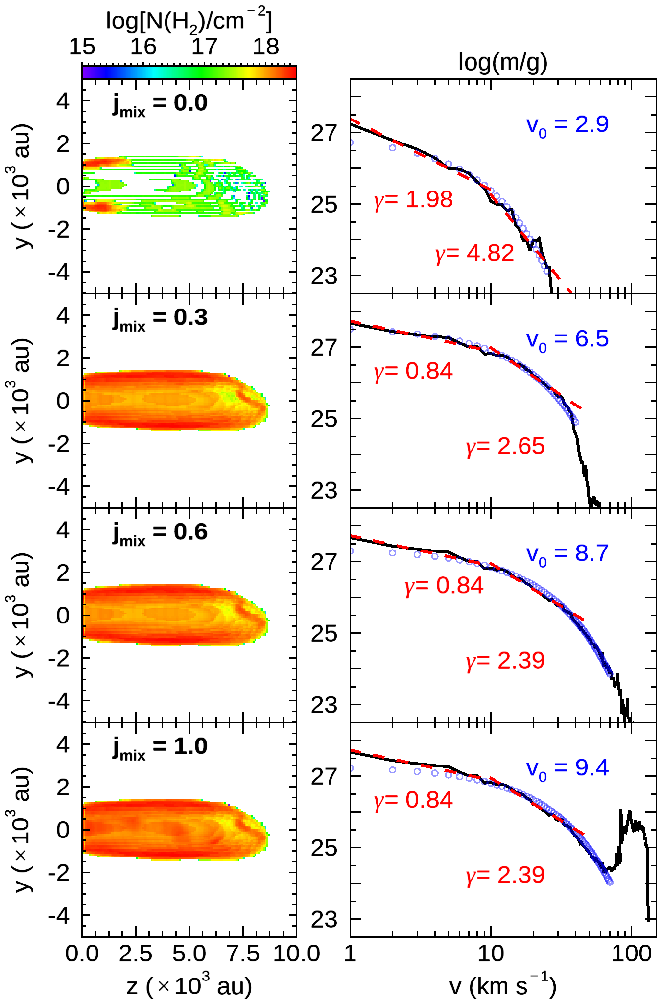
Figure 7: Model DR_P at $t=400$ yr and an inclination angle $i$= $30^{\circ}$. Results are presented for four different values of the jet–ambient gas mixing degree $j_{mix}$ (from top to bottom): 0.0, 0.3, 0.6, 1.0. (left) Maps of H₂ column density obtained by integration over the velocity range between 1 and $+150\hbox{\kern 1.99997ptkm\kern 1.99997pts${}^{-1}$}$. (right) Molecular mass–velocity relationship (black). The best-fitting power laws for the two velocity intervals: $v\leq 10\hbox{\kern 1.99997ptkm\kern 1.99997pts${}^{-1}$}$ (left) and $10<v\lesssim 20\hbox{\kern 1.99997ptkm\kern 1.99997pts${}^{-1}$}$ are drawn in dashed red. The index $\gamma$ is shown inside the panel. The exponential best fit is drawn in blue and the exponent $v_{0}$ is given for each $j_{mix}$ value.

The cavity created by the precessing jet appears broader close to the apex when compared with unprecesssing models, either intermittent (model DR; Fig. 5) or SS (model DR_SS; Fig. 6). Interestingly, both the molecular and total mass–velocity distributions are very similar to those obtained in the case of a pulsating, nonprecessing jet (Fig. 5) and a SS jet ( Fig. 6). The same two bumps at $v\sim 50\hbox{\kern 1.99997ptkm\kern 1.99997pts${}^{-1}$}$ and $v\sim 100\hbox{\kern 1.99997ptkm\kern 1.99997pts${}^{-1}$}$ are also detected in the total mass–velocity distribution (not shown in Fig. 7). In summary, the mass–velocity relationship is not significantly altered by jet precession and is very similar to that of nonprecessing, eventually pulsating jets.

4.3 Exponential fitting approach

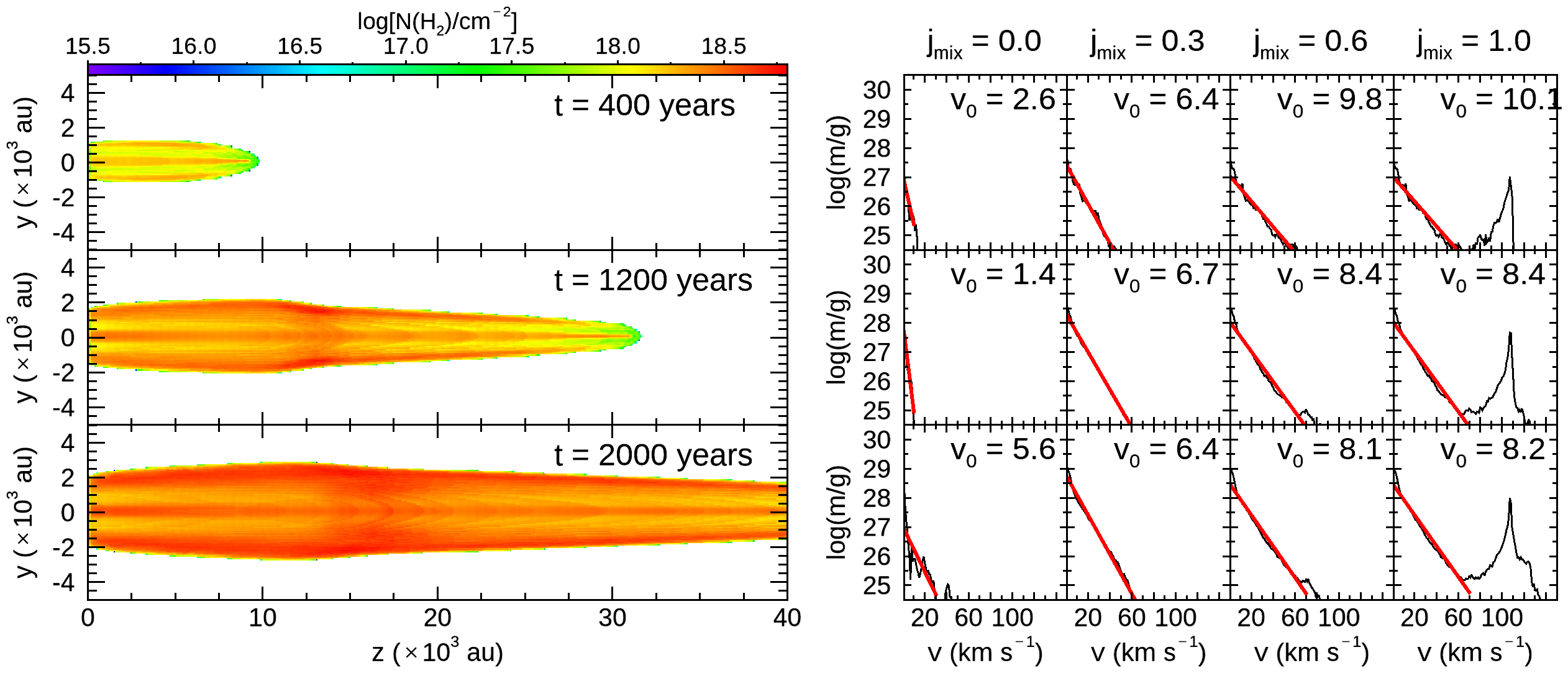
Figure 8: Model DR_SS at $t$ = 400, 1200 and 2000 years (from top to bottom) and for an inclination angle $i=30^{\circ}$. (Left) Distribution of molecular gas column density. (Right) The mass–velocity relationship is depicted in black for each value of the $j_{mix}$ parameter, from $j_{mix}=0.0$ (first column) to $j_{mix}=1.0$ (fourth column). The profiles were calculated considering the whole computational domain. The exponential best fit is drawn in red and the exponent $v_{0}$ is given for each $j_{mix}$ value.

Above, we compare and analyze the results of our simulations by modeling the mass–velocity distribution with a power law, $m(v)\propto v^{-\gamma}$. However, observational work on several molecular outflows by Lefloch et al. (2012) suggests that it could be possible to adopt another fitting, namely an exponential law $m(v)\propto\exp(-v/v_{0})$. Based on our numerical simulations, we assessed the validity of this approach.

We show the results of the fitting procedure for model DR_SS (Fig. 8) and model DR_P (Fig. 9) at the different times $t$ = 400, 1200, and $2000\hbox{\kern 1.99997ptyr},$ and, as in the preceding analyses, for four values of the jet–ambient gas mixing ratio $j_{mix}$= 0.0, 0,3, 0.6, 1.0. We adopted an inclination angle of $i=30^{\circ}$. We first consider the H₂ column density distribution and the molecular mass–velocity relationships resulting from the propagation of a steady-state jet (model DR_SS) . The value of the coefficient $v_{0}$ is indicated in each panel.

Our first result is that it is indeed possible to obtain a very good fit between the mass–velocity relationship and an exponential function $m(v)\propto{\rm exp}(-v/v_{0})$ from early ($400\hbox{\kern 1.99997ptyr}$) to late ($2000\hbox{\kern 1.99997ptyr}$) computational times (see Figs. 8–9), although the shallower $\gamma$ index in a power-law fitting translates into a higher $v_{0}$ value. The value of $v_{0}$ therefore increases with the jet–ambient gas mixing ratio. Our simulations for DR_SS (Fig 8) and DR_P (Fig. 9) show that higher values of $v_{0}$ are found at earlier times ($400\hbox{\kern 1.99997ptyr}$). Also, the best-fitting values of $v_{0}$ for both models DR_SS (Fig. 8) and DR_P (Fig. 9) under the same inclination angle are similar at the different times in the simulations, at 400, 1200, and $2000\hbox{\kern 1.99997ptyr}$. In other words, regardless of the age of the system, once a minimum level of mixing occurs between the jet and the ambient medium gas ($j_{mix}\geq 0.3$), the mass–velocity relationship and the value $v_{0}$ are almost unchanged. However, one can observe a small decrease of $v_{0}$ as time increases.

Close inspection of the mass–velocity relationships reveals that the exponential fitting (red curves) provides excellent solutions over the whole velocity range for $j_{mix}$ values of 0.3. For higher values of $j_{mix}$, the high-velocity range of the distribution $v\geq 10\hbox{\kern 1.99997ptkm\kern 1.99997pts${}^{-1}$}$ is still accurately fitted, with a higher value of $v_{0}$, as can be seen in Fig. 9 (e.g., panels $j_{mix}$=0.6). This expresses the fact that the jet contribution tends to make the mass–velocity distribution shallower, as discussed above. On the other hand, the slopes in the intermediate velocity range depend on the mixing level, and we identify two mechanisms that may explain this: the lack of material for $v\gtrsim 10$ km s^-1 in the case of swept-up H₂ profiles (case $j_{mix}=0.0$) and the presence of the jet as a bump at $v\simeq 40$ km s^-1 for $j_{mix}=1.0$. Between these two extremes we find great variability. We note that some residual emission is found in the low-velocity ($1<v<20\hbox{\kern 1.99997ptkm\kern 1.99997pts${}^{-1}$}$) range of the distribution, which can be fitted by two exponential functions. This point is addressed in more detail in the following paragraph.

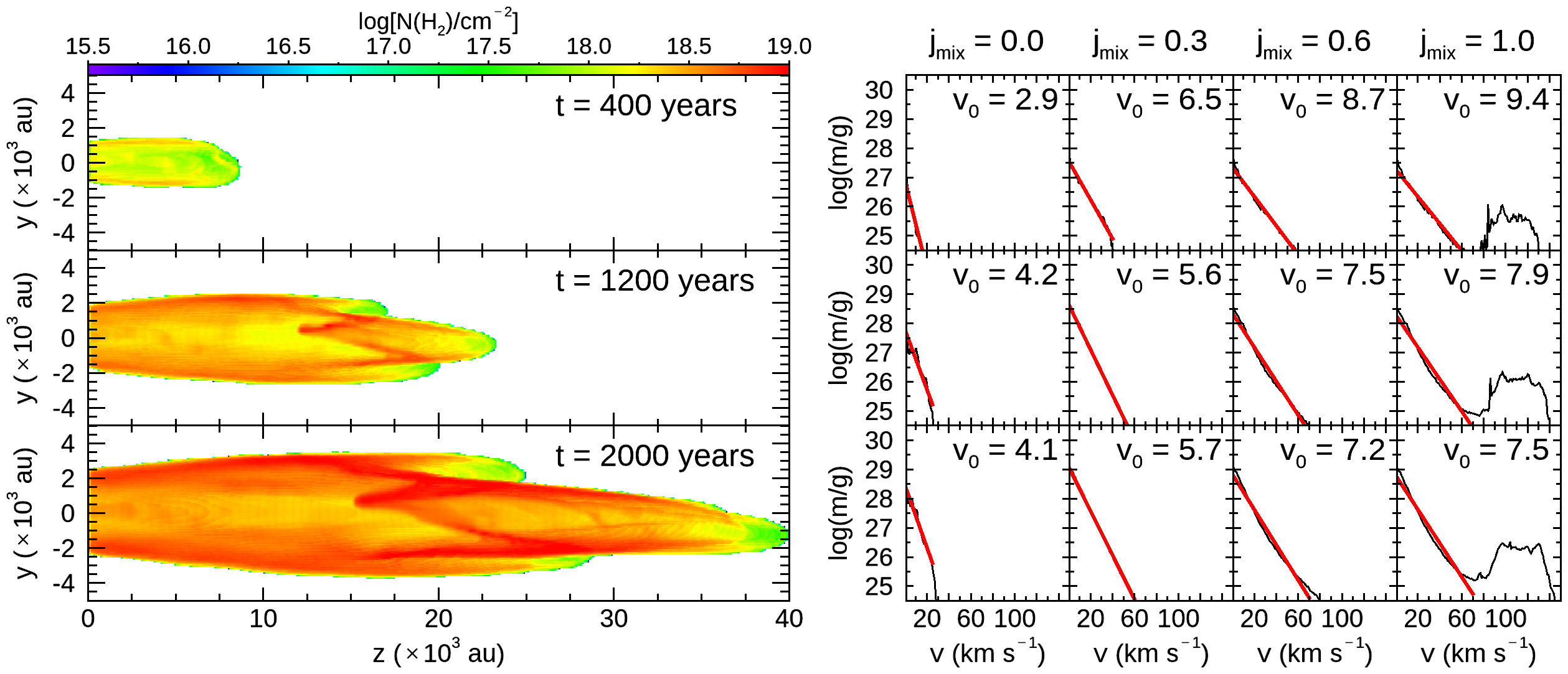
Figure 9: Model DR_P at $t$ = 400, 1200, and 2000 yr and for an inclination angle of $i=30^{\circ}$. The results are presented for four different values of the jet–ambient gas mixing degree $j_{mix}$ (from top to bottom): 0.0, 0.3, 0.6, 1.0. (left) Maps of H₂ column density obtained by integration over the velocity range between 1 and $+150\hbox{\kern 1.99997ptkm\kern 1.99997pts${}^{-1}$}$. (right) Mass–velocity relationship obtained for the molecular gas (black) and the fitted curve (red). The exponent $v_{0}$ is given for each $j_{mix}$ value.

4.4 From large- to small-scale

The results that we have discussed so far refer to the global mass–velocity relationship computed over the whole computational domain. However, the possibility of a local exponential fitting was reported by Lefloch et al. (2012) thanks to CO multi-line observations of the shock position B1 in the southern lobe of the L1157 outflow. These latter authors noticed that similar spectral signatures in the CO $J$=3–2 line were also detected at various other positions along the cavity walls of the L1157 outflow. This leads us to speculate that these spectral signatures could be a local property of the outfowing gas, and not only a global property, as has been considered until now. The goal of this section is to explore this point further.

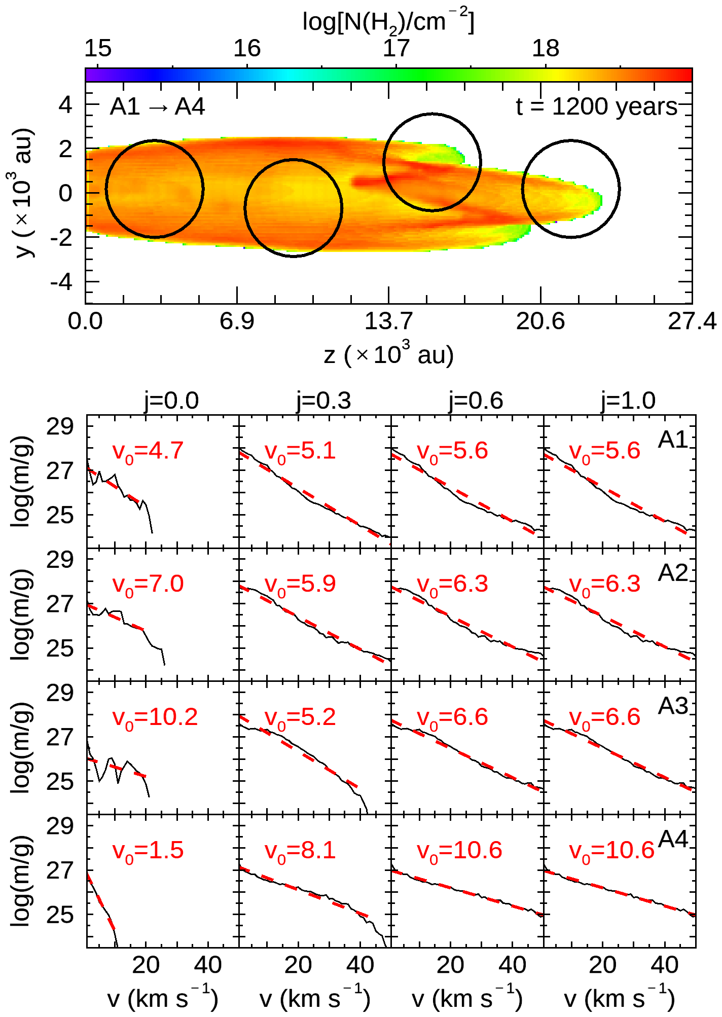
Figure 10: Model DR_P at $t$=$1200\hbox{\kern 1.99997ptyr}$ under an inclination of $30^{\circ}$. (top) Map of H₂ column density for $j_{mix}=1.0$. The location of the apertures A1-A4 used to extract the mass–velocity relationships are drawn with black circles. (bottom) Mass–velocity relationship averaged over the circular apertures A1 to A4. The best exponential fits are drawn in dashed red. The value of $v_{0}$ is given for each value of jet–ambient material mixing ratio $j_{mix}$= 0, 0.3, 0.6, 1.0.

In order to investigate the local behavior of the mass–velocity relationship, we considered the simulation of the outflowing gas in model DR_P at $t=1200\hbox{\kern 1.99997ptyr}$, with an inclination angle of $i=30^{\circ}$ and $j_{mix}=1.0$. We selected four positions in the outflow, labeled A1 to A4 and marked with black circles in the map of molecular gas column density in Fig. 10. While positions A1 and A2 are located inside the outflow cavity with A1 close to the jet main axis, positions A3 and A4 are located at shocked positions at the interface between the outflow and the ambient gas. We computed the molecular mass–velocity relationships over circular areas of $\sim$ 5000 au diameter at the four positions. The relationships and the best fits are displayed in the bottom panel of Fig. 10.

We verified that similar trends and results are found if we consider an aperture larger than 5000 au. However, profiles of the mass–velocity distribution become irregular (”noisy”) when the aperture size can no longer be considered large enough in comparison with the numerical resolution of the simulation.

Our first finding is that, at all four positions, the mass–velocity distribution can be well approximated by an exponential fit $m(v)\propto\exp(-v/v_{0})$. Hence, our simulations show that the exponential shape of the mass–velocity distribution in the outflow is a rather general result. We note that distributions are somewhat irregular when considering only the ambient material ($j_{mix}$=0). As soon as some degree of mixing is allowed between the jet and the ambient gas, an exponential fitting provides a very satisfying solution to the mass–velocity distribution at all positions. At first sight, similar distributions are obtained for positions A1 to A3, with values of $v_{0}\sim$ 5.1-6.6 km s^-1. These values are also similar to those of the global outflow mass–velocity distribution, as displayed in Fig. 9.

A higher value of $v_{0}$ of the order of 10 km s^-1 is found at position A4, close to the apex of the outflow cavity. Hence, it appears that if we leave aside the head of the outflow, the mass–velocity distributions display only modest variations across the outflow cavity, and do not bear signatures of the ejection process (intermittency, precession).

A closer look at the distributions shows that the mass–velocity distributions are better described by two components towards positions A1 to A3, with a change of slope (index) near $v=25\hbox{\kern 1.99997ptkm\kern 1.99997pts${}^{-1}$}$. In the high-velocity range, a shallower distribution is observed, which is related to the jet-entrained material. In order to explore the sensitivity of the fitting parameters to the geometry and the age of the outflow, we extracted the mass–velocity relationships at positions A1-A4 at three different times in the simulation of model DR_P, namely 400, 1200, and $2000\hbox{\kern 1.99997ptyr}$, and for three values of the inclination angle with respect to the plane of the sky: $i=$ 10, 30, and 60^∘. The fitting results of the mass–velocity relationships are summarized in Table 2.

Table 2: Model DR_P. Best exponential fitting parameters to the molecular mass–velocity distributions obtained towards positions A1–A4 in an aperture of 5000 au at $t$= 400, 1200, and $2000\hbox{\kern 1.79997ptyr}$, for three values of inclination angle: $i$=10^∘, 30^∘, and 60^∘.

$j_{mix}$	Age	Aperture	$v_{0}$ (kms-1)
	(years)		$i=10^{\circ}$	$i=30^{\circ}$	$i=60^{\circ}$
0.0	400	A1	1.3	2.7	4.4
		A2	1.3	2.6	4.4
		A3	1.4	2.6	2.0
		A4	1.1	1.3	1.9
	1200	A1	3.8	4.7	5.2
		A2	9.4	7.0	4.8
		A3	10.0	10.2	3.9
		A4	1.0	1.5	2.1
	2000	A1	2.8	3.1	4.9
		A2	2.7	4.2	4.9
		A3	2.8	4.8	4.9
		A4	3.2	5.9	1.8
$v_{i}\pm\sigma_{v_{i}}$ (kms-1):			3.4 $\pm$ 3.1	4.2 $\pm$ 2.6	3.8 $\pm$ 1.4
0.3	400	A1	3.3	4.9	9.2
		A2	3.2	4.8	10.6
		A3	3.2	5.9	11.5
		A4	4.3	6.0	13.8
	1200	A1	2.2	5.1	7.2
		A2	2.3	5.9	8.1
		A3	2.6	5.2	11.6
		A4	3.7	8.1	13.2
	2000	A1	2.6	5.3	7.8
		A2	2.4	5.9	7.9
		A3	2.7	4.4	8.4
		A4	2.5	5.5	15.0
$v_{i}\pm\sigma_{v_{i}}$ (kms-1):			2.9 $\pm$ 0.6	5.6 $\pm$ 1.0	10.4 $\pm$ 2.6
0.6	400	A1	3.2	6.5	9.6
		A2	3.2	6.5	11.3
		A3	3.1	7.3	13.0
		A4	4.0	9.0	15.5
	1200	A1	2.8	5.6	7.2
		A2	2.9	6.3	8.2
		A3	2.9	6.6	11.1
		A4	3.6	10.6	14.2
	2000	A1	2.8	5.5	7.8
		A2	3.0	6.1	8.0
		A3	2.9	5.6	8.6
		A4	2.7	6.6	15.2
$v_{i}\pm\sigma_{v_{i}}$ (kms-1):			3.1 $\pm$ 0.4	6.9 $\pm$ 1.5	10.8 $\pm$ 3.0
1.0	400	A1	5.9	6.6	9.6
		A2	6.2	6.5	11.3
		A3	7.0	7.3	13.0
		A4	6.5	9.0	15.5
	1200	A1	4.8	5.6	7.2
		A2	4.1	6.3	8.2
		A3	4.5	6.6	11.1
		A4	4.4	10.6	14.2
	2000	A1	4.5	5.5	7.8
		A2	4.7	6.1	8.0
		A3	3.9	5.6	8.6
		A4	3.4	6.7	15.2
$v_{i}\pm\sigma_{v_{i}}$ (kms-1):			5.0 $\pm$ 1.1	6.9 $\pm$ 1.5	10.8 $\pm$ 3.0

5 Discussion

5.1 Molecular outflows

Lefloch et al. (2012) modeled the observed intensity–velocity distribution $I_{\rm CO}$ of the five outflow sources previously observed by Bachiller & Tafalla (1999): Mon R2, L1551, NGC2071, Orion A, and L1448. These latter authors showed that the observed $I_{\rm CO}$ could be well fitted by an exponential function with values of $v_{0}$ between 1.6 (Mon R2) and 12.5 (L1448) kms^-1.

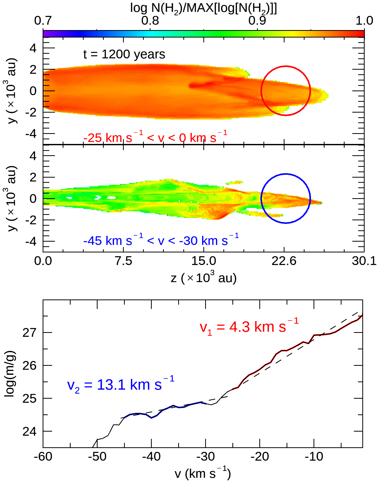
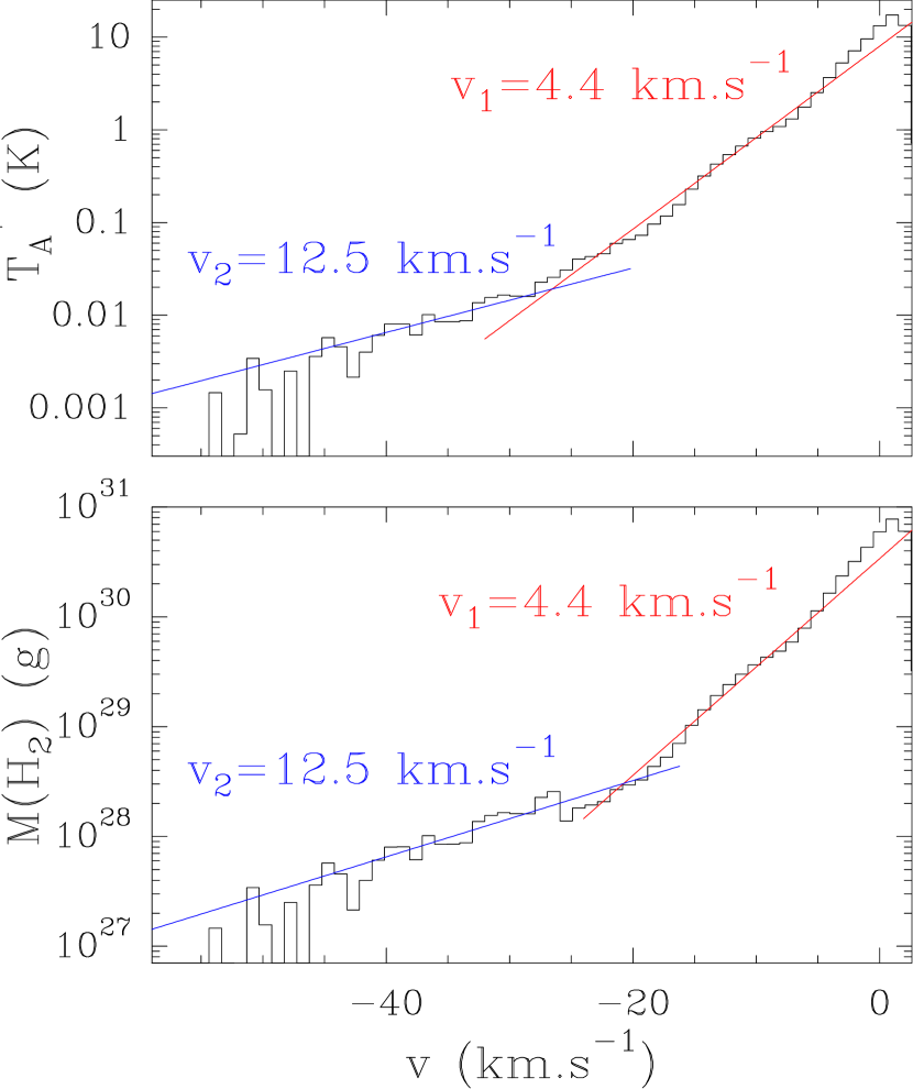
Figure 11: (Left) Model DR_P at $t$=$1200\hbox{\kern 1.99997ptyr}$ under an inclination of $10^{\circ}$ (towards the observer). (top) Map of H₂ column density for $j_{mix}=0.9$, in the velocity intervals $-[1-25\hbox{\kern 1.99997ptkm\kern 1.99997pts${}^{-1}$}]$ (top) and $-[30-45\hbox{\kern 1.99997ptkm\kern 1.99997pts${}^{-1}$}]$ (bottom). The 5000 au aperture used to extract the mass–velocity distribution is drawn by a circle. (bottom) Molecular mass–velocity distribution extracted at position A4. We have superposed the best exponential fits $m(v)\propto\exp(-v/v_{i})$ to the components associated with velocity intervals $-[1-25\hbox{\kern 1.99997ptkm\kern 1.99997pts${}^{-1}$}]$ (red) and $-[30-45\hbox{\kern 1.99997ptkm\kern 1.99997pts${}^{-1}$}]$ (blue). The exponent value $v_{i}$ is given for both velocity intervals. (Right) ASAI observations of L1157-B1. (top) Intensity–velocity distribution obtained in the CO $J$=2–1 towards shock position B1 in an aperture of about 4000 au (11″at the distance to the source). The line profile is fitted by a linear combination of two exponential functions $g_{1}\propto\exp(-v/12.5)$ (blue), $g_{2}\propto\exp(-v/4.4)$ (red) (from Lefloch et al., 2012). (bottom) Associated mass–velocity distribution, adopting a standard CO-to-H₂ abundance ratio and the excitation conditions derived by Lefloch et al. (2012) for the velocity components $g_{1}$ and $g_{2}$.

A quick inspection of the grid of models presented in Table 2 shows that these values fall well within the range of values predicted in our simulations, depending on the outflow age, the inclination angle, and the degree of jet–ambient gas mixing ratio. A value as low as 1.6 for Mon R2 is indeed easily accounted for if the outflow propagates close to the plane of the sky, as proposed by DC03. For an inclination angle of $10^{\circ}$, and a time of 1200-$2000\hbox{\kern 1.99997ptyr}$, our modeling predicts low values $v_{0}\sim 1.5-2.0$, which are easily obtained where there is a lack of entrainment in the outflowing gas ($j_{mix}$=0.0). We note that these values are not very sensitive to the actual age of the outflow (time of the simulation).

The young sources Orion A and L1448, with an estimated age of $1000\hbox{\kern 1.99997ptyr}$, are best fitted with $v_{0}$ values of $6.6$ and $12.5\hbox{\kern 1.99997ptkm\kern 1.99997pts${}^{-1}$}$ (according to Lefloch et al., 2012). These values of $v_{0}$ are easily accounted for in the simulations at early ages (400-$1000\hbox{\kern 1.99997ptyr}$) with an inclination angle of 60^∘. Solutions with a lower inclination angle and a different degree of jet–ambient gas mixing ratio are possible. Detailed modeling of the sources is necessary to disentangle the impact of the different parameters. Interestingly, the spectra for L1448 presented in Fig. 4 in Lefloch et al. (2012) present a bump at $v\sim 60\hbox{\kern 1.99997ptkm\kern 1.99997pts${}^{-1}$}$, which we interpret as the signature of the driving jet.

From comparison with the outflow sample of Bachiller & Tafalla (1999), a scenario emerges in which more-evolved sources (like Mon R2) are better described by the swept-up gas (i.e, no entrainment; $j_{mix}=0$), while younger sources unveil the ambient medium entrained by the jet, making the profiles shallower and consistent with $v_{0}\sim 10\hbox{\kern 1.99997ptkm\kern 1.99997pts${}^{-1}$}$.

5.2 Mass–velocity relationships in the L1157 outflow

In this section, we apply our numerical models to L1157 in order to better understand the origin of the CO intensity–velocity distributions reported by Lefloch et al. (2012) in the southern outflow lobe of L1157. We note that our goal is not to provide a detailed modeling of the L1157 southern outflow lobe. For this reason, we focus on the signatures associated with the B1 outflow cavity.

As mentioned in Section 3.2, the simulation parameters of model DR_P were chosen to describe the behavior of a ”typical” precessing jet. For this reason, and taking into account the simplicity of the underlying hypothesis of our model, we did not attempt to fine-tune the simulation parameters in order to obtain the ”best-fitting” model.

5.2.1 Multiple components

As mentioned in Section 2, several authors have investigated the details of the CO emission from the southern lobe of the L1157 outflow. As first shown by Gueth, Guilloteau & Bachiller (1996), the precessing protostellar jet has shaped the southern lobe into two shells (outflow cavities) whose apexes are associated with the molecular shock positions B1 and B2. Detailed modeling of the CO gas kinematics by Podio et al. (2016) showed that the jet precesses on a cone inclined by $73^{\circ}$ to the line of sight, with an opening angle of $8^{\circ}$ on a period of $1640\hbox{\kern 1.99997ptyr}$. The modeling of the authors indicates that an angle of $\approx 10^{\circ}$ exists between the jet and the line of sight at the location of B1.

The top-right panel of Fig. 11 shows the CO intensity–velocity distribution as observed in the $J$=2–1 line with IRAM-30m (Lefloch et al., 2012). From a multi-transition analysis of the CO line profiles, these latter authors found the following results:

• The CO line profiles profiles are the sum of up to three components of specific excitation and velocity range, dubbed $g_{1}$, $g_{2}$, $g_{3}$, all of which can be modeled by an exponential law with a specific exponent $v_{0}$: 12.5, 4.4, 2.5, respectively.

• The component of lowest excitation ($T_{ex}$=$23\hbox{\kern 1.99997ptK}$) and narrowest velocity range, ($-5;0\hbox{\kern 1.99997ptkm\kern 1.99997pts${}^{-1}$}$), dubbed $g_{3}$, is detected over the whole southern lobe and is the only component detected towards the southernmost, older cavity associated with the B2 shock.

• The component of highest excitation ($T_{ex}$=$210\hbox{\kern 1.99997ptK}$) and highest velocity range, $[-40;-20]\hbox{\kern 1.99997ptkm\kern 1.99997pts${}^{-1}$}$, dubbed $g_{1}$, is detected close to the apex of the younger cavity associated with the B1 shock.

• The component of intermediate excitation ($T_{ex}$=$64\hbox{\kern 1.99997ptK}$) and velocity range, $-20<v<-5\hbox{\kern 1.99997ptkm\kern 1.99997pts${}^{-1}$}$, dubbed $g_{2}$ is detected over the whole outflow cavity associated with B1.

5.2.2 Observational derivation of m(v)

The excitation conditions of the CO gas in L1157 make it especially easy to obtain the mass–velocity distribution from the CO intensity–velocity distribution. This is because the CO $J$=2–1 excitation conditions of each component $g_{1}$, $g_{2}$, $g_{3}$ are independent of the velocity and the line emission is optically thin, but at velocities very close (a few kms^-1) to ambient. Hence, the simple relation that exists at local thermodynamic equilibrium between N(CO) and the CO line flux (see e.g., Bachiller et al., 1990) can be applied to the whole velocity range of emission of each component. In practice, each component dominates over a specific velocity interval of the intensity–velocity distribution (see top right panel of Fig. 11). The mass–velocity distribution is therefore immediately obtained when considering the excitation conditions and the size of the main emitting gas component as a function of velocity. The total mass–velocity relationship is rigorously obtained by multiplying the relationship N(CO)(v) —which is derived from $T_{b}$(CO)(v)— by the CO emission area at each velocity interval. Despite the uncertainties in the overlap region between components (e.g., near $v=-25\hbox{\kern 1.99997ptkm\kern 1.99997pts${}^{-1}$}$), the spectral slope of each component is found to be preserved in the derivation procedure from the CO intensity to the mass–velocity distribution. This is illustrated in the bottom-right panel of Fig. 11 in which we report the mass–velocity distribution towards L1157-B1. We note that we assume a standard abundance ratio CO/[H₂]= $10^{-4}$.

5.2.3 Spatial distribution

Figure 11 presents the distributions of the molecular material in the velocity intervals $[-25;-1]\hbox{\kern 1.99997ptkm\kern 1.99997pts${}^{-1}$}$ (top) and $[-45;-30]\hbox{\kern 1.99997ptkm\kern 1.99997pts${}^{-1}$}$, respectively. We also computed the molecular mass–velocity distribution measured in an aperture of 5000 au close to the apex of the cavity (position A4). This is comparable to the beamwidth (HPBW) of the IRAM 30m telescope main beam at the frequency of the CO $J$=2–1 line.

Our simulations (see Fig. 10) show that after a few hundred years the intensity–velocity distribution is approximately uniform over the outflow cavity, except at the apex where the jet contribution is strongest. This is consistent with the detection of rather uniform signatures $g_{2}$ and $g_{3}$ over the B1 and B2 lobes, respectively. Our model DR_P is consistent with the interpretation that $g_{2}$ and $g_{3}$ are associated with different ejection events responsible for the formation of B1 and B2 cavities, respectively. The lower excitation conditions of $g_{3}$ are consistent with an older event. The difference of spectral slope ($v_{0}$) between the B1 and B2 cavities could be explained a priori by a higher jet inclination to the line of sight in the direction of B2. However, this contradicts the kinematic modeling of the jet precession by Podio et al. (2016), which predicts an inclination angle to the line of sight of about $25^{\circ}$ at shock position B2, lower than towards B1, and therefore favors a higher jet radial velocity than that measured towards B1. The sensitivity of the millimeter CO line spectra available in the literature (see e.g., Lefloch et al., 2012) is not high enough to allow conclusions to be made about the presence of the jet towards B2. On the other hand, our numerical simulations show that the low-velocity ($v<5\hbox{\kern 1.99997ptkm\kern 1.99997pts${}^{-1}$}$) emission actually arises from entrained ambient material in the outflow cavity walls, and has very little dependence on the driving jet. The jet that once created the B2 shock about $2500\hbox{\kern 1.99997ptyr}$ ago (Podio et al., 2016) is now impacting the B1 cavity at the B1 and B0 positions as a result of its precession. Hence, the emission from B2 arises mainly from previously entrained, ambient material, which is now being slowed down. Inspection of Table 2 shows that low values of $v_{0}$ are also obtained in the swept-up ambient molecular gas ($j_{mix}=0.0$).

5.2.4 Jet signature

As can be seen in Fig. 11, the mass–velocity distribution extracted towards position A4, close to the apex of the cavity in the simulation, shows the presence of two distinct components associated with the velocity intervals [$-1;-25\hbox{\kern 1.99997ptkm\kern 1.99997pts${}^{-1}$}$] and [$-30;-45\hbox{\kern 1.99997ptkm\kern 1.99997pts${}^{-1}$}$], respectively. This situation is reminiscent of the CO (and the mass) intensity–velocity distribution observed towards B1. Both components can be fitted by an exponential function of exponent $v_{0}\simeq 4.3$ and $v_{0}\simeq 13$, respectively. These values are in good agreement with those determined for components $g_{2}$ and $g_{1}$ towards the B1 position. We note that according to our modeling (see Table 2), these values are mainly sensitive to the jet inclination angle to the line of sight. We note that they weakly depend on the actual value of the jet–ambient material mixing ratio, but the best agreement was obtained for $j_{mix}$= 0.9.

In our simulation, the distribution of the high-velocity material between -45 and $-30\hbox{\kern 1.99997ptkm\kern 1.99997pts${}^{-1}$}$, as displayed in Fig. 11, is not restricted to a few spots of shocked gas, such as for example the jet impact shock region at the apex of the outflow cavity. Instead, it turns out that the high-velocity material ($|v|>30\hbox{\kern 1.99997ptkm\kern 1.99997pts${}^{-1}$}$) is tracing an elongated, collimated structure surrounding the jet throughout the whole outflow cavity. This elongated structure is surrounded by the lower velocity material ($0<|v|<25\hbox{\kern 1.99997ptkm\kern 1.99997pts${}^{-1}$}$) of the outflow. In other words, the high-velocity material does not trace only the jet shock impact region (the Mach disk). In our simulation, the amount of molecular material at the jet head strongly decreases as a result of molecular dissociation. Instead, the high-velocity component arises from material entrained along the jet.

5.2.5 Observational predictions for the high-velocity gas

Observational evidence of the high-velocity component has been reported in the millimeter rotational transitions of a few molecular species, such as for example CO (Lefloch et al., 2012), HCO⁺ (Podio et al., 2014), and SiO (Tafalla et al., 2010; Spezzano et al., 2020). Unfortunately, the interferometric observations of L1157 available in the literature focus mainly on the gas propagating at velocities close to ambient, which is associated with the bow and the outflow cavity walls. Therefore, the evidence for the high-velocity jet is still very scarce and unambiguous detection of the molecular material entrained along the jet is still missing. It is worth noting that Plateau de Bure observations of the SiO $J$=2–1 line by Gueth, Guilloteau & Bachiller (1998) revealed an elongated , ”jet and filamentary-like” feature for gas emitting at $v<-10\hbox{\kern 1.99997ptkm\kern 1.99997pts${}^{-1}$}$. Single-dish observations of the SiO $J$=2–1 line indicate that this feature displays the expected intensity–velocity distribution, as shown by Lefloch et al. (2012). We speculate that this feature might well be the signature of the molecular jet and not the jet impact shock region itself.

This conclusion could be easily verified (or disproved) by high-angular resolution observations of the CO or SiO millimeter line emission with the IRAM interferometer NOEMA. According to our modeling, the high-velocity emission should reveal a collimated, filamentary-like structure. In the opposite case, that is, if the gas is accelerated in the jet impact shock region, the high-velocity emission should trace the compact region associated with the Mach disk.

6 Conclusions

Using the hydrodynamical code Yguazú-a, we performed 3D numerical simulations to revisit in a detailed manner the mass–velocity relationship in jet-driven molecular outflows. Great attention was paid to benchmark Yguazu-a against the hydrodynamical codes used by previous authors in the field (Downes & Ray, 1999; Downes & Cabrit, 2003). To do so, we modeled the propagation of an intermittent jet adopting the same parameters as those of Downes & Ray (1999) and Downes & Cabrit (2003). We find excellent quantitative agreement between our simulations and those of these latter authors.

Detailed comparison between our simulations and those of Downes & Cabrit (2003) leads us to conclude that these latter authors took into account the jet material contribution in the obtention of the mass–velocity distribution presented in their work. We find that the presence of a bump in the high-velocity range ($v\sim 100\hbox{\kern 1.99997ptkm\kern 1.99997pts${}^{-1}$}$) is remarkable evidence of the presence of the jet and that all the previous works considered, to a greater or lesser extent, the presence of the jet in their mass–velocity profile computations.

Overall, our simulations show that the mass–velocity distribution of the outflowing material can be successfully fitted by one exponential law $m(v)\propto\exp(-v/v_{0})$. We systematically investigated the signature of the mass–velocity distribution as a function of time, depending on the jet inclination to the line of sight and the degree of mixing between the jet and the ambient material. We find that it may be necessary to introduce a second component to fit the mass–velocity distribution in the high-velocity range. The spectral signature in the low-velocity range is dominated by the contribution of material in the outflow cavity walls and is rather insensitive to the actual value of the jet–ambient gas mixing ratio. The synthetic mass–velocity distributions from our simulations are good agreement with distributions derived from observations and we are able to reproduce the observational data when taking age and source geometry into account.

We verified that the profile of the mass–velocity distribution computed over a local area inside the outflow can still be well fitted by an exponential function. The profiles and the $v_{0}$ values are very similar over the outflow, but the distribution appears much shallower at the apex of the outflow cavity as a result of the leading jet contribution.

We performed a simple modeling of the L1157 southern outflow cavity by simulating of a precessing jet with parameters similar to those reported by Podio et al. (2016). We were able to reproduce the main features of the CO intensity–velocity distributions observed in the southern outflow lobe of L1157 to a satisfactory degree. Our simulations suggest that the three components identified by Lefloch et al. (2012) are all related to the entrained gas and not the jet impact shock region, that is, the Mach disk itself. High-angular-resolution observations with the NOEMA interferometer could easily test this conclusion.