String Tightening as a Self-Organizing Phenomenon:
Computation of Shortest Homotopic Path, Smooth Path, and Convex Hull

Abstract

The phenomenon of self-organization has been of special interest to the neural network community for decades. In this paper, we study a variant of the Self-Organizing Map (SOM) that models the phenomenon of self-organization of the particles forming a string when the string is tightened from one or both ends. The proposed variant, called the String Tightening Self-Organizing Neural Network (STON), can be used to solve certain practical problems, such as computation of shortest homotopic paths, smoothing paths to avoid sharp turns, and computation of convex hull. These problems are of considerable interest in computational geometry, robotics path planning, AI (diagrammatic reasoning), VLSI routing, and geographical information systems. Given a set of obstacles and a string with two fixed terminal points in a two dimensional space, the STON model continuously tightens the given string until the unique shortest configuration in terms of the Euclidean metric is reached. The STON minimizes the total length of a string on convergence by dynamically creating and selecting feature vectors in a competitive manner. Proof of correctness of this anytime algorithm and experimental results obtained by its deployment are presented in the paper.

Index terms— Path planning, homotopy, shortest path, convex hull, smooth path, self organization, neural network.

1 Introduction

Self-organization, as a phenomenon, has received considerable attention from the neural network community in the last couple of decades. Several attempts have been made to use neural networks to model different self-organization phenomena. One of the most well known of such attempts is that of Kohonen’s who proposed the Self-Organizing Map (SOM) [2] inspired by the way in which various human sensory impressions are topographically mapped into the neurons of the brain. SOM possesses the capability to extract features from a multidimensional data set by creating a vector quantizer by adjusting weights from common input nodes to M output nodes arranged in a two dimensional grid. At convergence, the weights specify the clusters or vector centers of the set of input vectors such that the point density function of the vector centers tend to approximate the probability density function of the input vectors. Several authors in different contexts reported different dynamic versions of SOM [2, 3, 4, 5, 6, 7, 8, 9, 10, 11].

In this paper, assuming a string is composed of a sequence of particles, we claim that the phenomenon undergone by the particles of the string, when the string is pulled from one or both ends to tighten it, is that of self-organization, by modeling the phenomenon using a variant of SOM, called the String Tightening Self-Organizing Neural Network (STON). We further use the proposed variant to solve a few well-known practical problems - computation of shortest path in a given homotopy class, smoothing paths to avoid sharp turns, and computation of convex hull. Other than theoretical considerations in computational geometry [12], computation of shortest homotopic paths is of considerable interest in robotics path-planning [13], AI (diagrammatic reasoning) [14, 15, 16, 17, 18, 19, 20, 21, 22, 23, 24], VLSI routing [25], and geographical information systems. Smooth paths are required for navigation of large robots incapable of taking sharp turns, and also for handling unexpected obstacles. To generate a path that is smooth, shorter, collision-free, and is homotopic to the original path requires generation of the configuration space of a robot which is computationally expensive and difficult to represent [26]. Computation of convex hull finds numerous applications in computational geometry algorithms, pattern recognition, image processing, and so on. The aim of this paper is to study the properties of STON and how it might be applied to solve some practical problems as described above.

The remainder of this paper is organized as follows. In the next section, the STON algorithm is described assuming the given string is sampled at a frequency of at least $d/2$ where $d$ is the minimum distance between the obstacles. Thereafter, an analysis of the algorithm is presented along with proof of its important properties and correctness. Section 4 discusses how STON might be extended when the above constraint on sampling is not met. The extension is used for computation of shortest path in a given homotopy class. Proof of correctness and complexity analysis of the extension are also included. Finally, simulation results are presented from computing shortest homotopic path, smooth path and convex hull using both the original and extended algorithms. The paper concludes with a general discussion.

2 The STON Algorithm

2.1 Homotopy

A string $\pi$ in two dimensional space $(\Re^{2})$ might be defined as a continuous mapping $\pi:[0,1]\rightarrow\Re^{2}$, where $\pi(0)$ and $\pi(1)$ are the two terminal points of the string. A string is simple if it does not intersect itself, otherwise it is non-simple. Let $\pi_{1}$ and $\pi_{2}$ be two strings in $\Re^{2}$ sharing the same terminal points i.e. $\pi_{1}(0)=\pi_{2}(0)$ and $\pi_{1}(1)=\pi_{2}(1)$, and avoiding a set of obstacles $P\subset\Re^{2}$. The strings $\pi_{1}$, $\pi_{2}$ are considered to be homotopic to each other or to belong to the same homotopy class, with respect to the set of obstacles $P$, if there exists a continuous function $\Psi:[0,1]\times[0,1]\rightarrow\Re^{2}$ such that
1. $\Psi(0,t)=\pi_{1}(t)$ and $\Psi(1,t)=\pi_{2}(t)$, for $0\leq t\leq 1$
2. $\Psi(\lambda,0)=\pi_{1}(0)=\pi_{2}(0)$ and $\Psi(\lambda,1)=\pi_{1}(1)=\pi_{2}(1)$, for $0\leq\lambda\leq 1$
3. $\Psi(\lambda,t)\notin P$, for $0\leq\lambda\leq 1$ and $0\leq t\leq 1$.
Informally, two strings are considered to be homotopic with respect to a set of obstacles, if they share the same terminal points and one can be continuously deformed into the other without crossing any obstacle. Thus homotopy is an equivalence relation.

Given a string $\pi_{i}$, specified in terms of sampled points, and a set of obstacles $P$, STON computes a string $\pi_{s}$ such that $\pi_{i}$ and $\pi_{s}$ belong to the same homotopy class, and the Euclidean distance covered by $\pi_{s}$ is the shortest among all strings homotopic to $\pi_{i}$. It is noteworthy that $\pi_{s}$ is unique and has some canonical form [27].

2.2 The Objective

Assume a string wound around obstacles in $\Re^{2}$ with two fixed terminal points. A shorter configuration of the string can be obtained by pulling its terminals. The unique shortest configuration can be obtained by pulling its terminals until they cannot be pulled any more. The proposed algorithm models this phenomenon as a self-organized mapping of the points forming a given configuration of a string into points forming the desired shorter configuration of the string. Let us consider a set of $n$ data points or obstacles, $P=\{p_{1},p_{2},...p_{n}\}$, representing the input signals, and a sequence of variable (say, $k$) processors $\langle q_{1},q_{2},...q_{k}\rangle$ each of which (say $q_{i}$) is associated with a weight vector $w_{i}(t)$ at any time $t$. A weight vector represents the position of its processor in $\Re^{2}$. If the $k$ processors are placed on a string in $\Re^{2}$, the STON is an anytime algorithm for tuning the corresponding weights to different domains of the input signals such that, on convergence, the processors will be located in such a way that they minimize a distance function, $\phi(w)$, given by

$$\phi(w)=\displaystyle\sum_{i=1}^{k-1}\|w_{i+1}(t)-w_{i}(t)\|^{2}$$ (1)

where $q_{i}$, $q_{i+1}$ are two consecutive processors on the string with corresponding weights $w_{i}(t)$, $w_{i+1}(t)$ at any time $t$. The algorithm further guarantees that the final configuration of the string formed by the sequence of processors at convergence lies in the same homotopy class as the string formed by the initial sequence of processors with respect to $P$. Thus, assuming fixed $q_{1}$ and $q_{k}$, the STON defines the shortest configuration of the $k$ processors in an unsupervised manner. The phenomenon undergone by the particles forming the string is modeled by the processors in the neural network.

2.3 Initialization of the Network

The STON is initialized with a given number of connected processors, the weight corresponding to each of which is initialized at a unique point on the given configuration of a string. A feature vector, presented to the STON, is an attractor point in $\Re^{2}$ and is either created dynamically or chosen selectively from the given set of input obstacles $P$. The weight vectors are updated iteratively on the basis of the created and chosen feature space $S(t)$; $S(t)=\{x_{1}(t),x_{2}(t),...x_{k}(t)\}$ being the set of feature vectors at any time $t$. It is noteworthy that $x_{i}(t)$ is not necessarily unique. Unlike SOM and many of its variants, randomized updating of weights does not yield better results in the STON model; updating weights sequentially or randomly both yield the same result in terms of output quality as well as computation time. On convergence, the location of the processors representing the unique shortest configuration homotopic to the given configuration of the string is obtained.

2.4 Creating/Choosing Feature Vectors

A feature vector $x_{i}(t)$ is created if the triangular area spanned by three consecutive processors $q_{m-1}$, $q_{m}$, $q_{m+1}$ does not contain any obstacle $p_{j}\in P$. In that case,

$$x_{i}(t)=\frac{w_{m-1}(t^{\prime})+w_{m+1}(t^{\prime\prime})}{2}$$ (2)

where $t^{\prime}$, $t^{\prime\prime}$ assumes the value $t$ if the weight has not yet been updated in the current iteration or sweep and the value $t+1$ if the weight has been updated in the current sweep, and $1<m<k$. If an obstacle, say $p_{j}\in P$, lies within the triangular area spanned by the three consecutive processors $q_{m-1}$, $q_{m}$, $q_{m+1}$, the feature vector $x_{i}(t)$ is chosen to be

$$x_{i}(t)=p_{j}$$ (3)

For this algorithm, we assume the given string is sampled such that there cannot exist multiple non-identical obstacles within the triangular area spanned by any three consecutive processors (see Appendix A.1 for how to achieve such sampling).

2.5 Updating Weights

The STON evolves by means of a certain processor evolution mechanism, given by [28]

$$w_{m}(t+1)=w_{m}(t)+\alpha(t)[x_{j}(t)-w_{m}(t)]$$ (4)

where $\alpha(t)$ is the gain term or learning rate which might vary with time and $0\leq\alpha(t)\leq 1$. $\alpha(t)$ might be unity only when feature vectors are created according to eq. 2. All the weight vectors are updated exactly once in a single sweep, indexed by $t$.

If modification of weights is continued in this process, the processors tend to produce shorter configurations at the end of each sweep. The weight vectors converge when

$$\|w_{i+1}(t)-w_{i}(t)\|<\epsilon,\forall i$$ (5)

where $\epsilon$ is a predetermined sufficiently small positive scalar quantity.

3 Analysis of STON

STON is a variant of SOM. As in SOM, each feature vector in STON pulls the selected processors in a neighborhood towards itself as a result of updating in a topologically constrained manner, ultimately leading to an ordering of processors that minimizes some residual error. Neighborhood, in SOM, is something like a smoothing kernel over a two dimensional grid often taken as the Gaussian which shrinks over time. In STON, all those processors are included within the neighborhood of a feature vector that form triangles with their adjacent processors such that the feature vector lies within their triangles. Such a neighborhood is conceptually similar to that proposed in [29] where the neighborhood is not dependent on time but on the nature of the input signals. STON incorporates competitive learning as the weights adapt themselves to specific chosen features of the input signal defined in terms of the obstacles. The residual error is defined in SOM in terms of variance while in STON, in terms of Euclidean distance. From the inputs the net adapts itself dynamically in an unsupervised manner to acquire a stable structure at convergence, thereby manifesting self-organization [30]. The STON possesses certain key properties which are discussed in this section that eventually leads to the proof of correctness of the algorithm.

Theorem 1.

The configuration of a string formed by the sequence of processors at initialization and the same at convergence are homotopic.

Proof.

We start by noting that, given a fixed set of obstacles and fixed terminal points, the homotopy class of a string can be altered only by crossing any obstacle. The configuration of a string formed by the sequence of processors at any time $t$ is obtained by updating the weights with respect to the selected feature vectors at time $t$-1, the feature vectors being selected according to eq. 2 or 3. In the first case, creation of a feature vector and updating the weight does not change the homotopy class of the string as there was no obstacle in the triangular area, hence updating the weight did not result in crossing any obstacle.

In the second case, a feature vector is selected by eq. 3 from the set of obstacles. A processor is pulled towards the feature vector by updating its weight. It requires to be proven that by such selection of feature vectors and updating of weights, a string cannot cross any obstacle. Let $q_{i-1}$, $q_{i}$, $q_{i+1}$ be three consecutive processors on a string with corresponding weights being $w_{i-1}(t^{\prime})$, $w_{i}(t)$, $w_{i+1}(t^{\prime\prime})$; $t^{\prime},t^{\prime\prime}\in\{t,t+1\}$, and $x_{i}(t)=p_{j}$ be the selected feature vector (see Fig. 1). In order to complete the proof we need to show $p_{j}$ will never be crossed if – (i) weight for processor $q_{i}$ is updated, and (ii) weight for one of the neighbors of $q_{i}$ (i.e. $q_{i-1}$ or $q_{i+1}$) is updated.

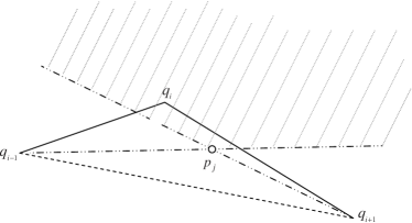
Figure 1: If $p_{j}$ lies inside the triangle formed by $q_{i-1}$, $q_{i}$, $q_{i+1}$, then $q_{i}$ has to lie in the shaded region.

First, note that in order for $p_{j}$ to be inside the triangle formed by $q_{i-1}$, $q_{i}$, $q_{i+1}$, the processor $q_{i}$ has to be in the region bounded by extensions of the lines joining $q_{i-1}$ and $q_{i+1}$ to $p_{j}$ (i.e. the shaded region in Fig. 1). Since updating the weight for processor $q_{i}$ pulls it towards the obstacle $p_{j}$ along a straight line, $q_{i}$ continues to remain within the shaded region after updating, thereby never letting the segments $\overline{q_{i-1}q_{i}}$ and $\overline{q_{i}q_{i+1}}$ cross the obstacle $p_{j}$. That proves condition (i).

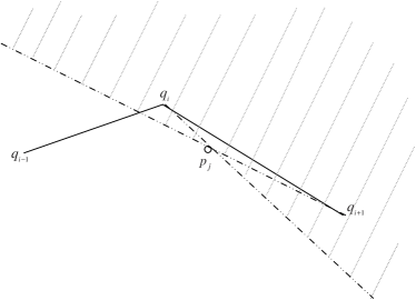
Figure 2: The feature vector for updating the weight for $q_{i+1}$, if not $p_{j}$, can lie only in the shaded region.

Now let us consider the case when the weight for a neighbor of $q_{i}$, say $q_{i+1}$ without loss of generality, is updated. Let $q_{i+2}$ be the other neighbor of $q_{i+1}$. Then either the obstacle $p_{j}$ lies inside the triangle formed by $q_{i}$, $q_{i+1}$, $q_{i+2}$, or it does not. If $p_{j}$ lies inside, it is the selected feature vector that pulls $q_{i+1}$ towards itself and it will never be crossed (due to condition (i)). If $p_{j}$ does not lie inside, then either there lies some other obstacle, say $p_{j^{\prime}}$, inside the triangle formed by $q_{i}$, $q_{i+1}$, $q_{i+2}$, or there does not exist any obstacle inside. In the former case, $p_{j^{\prime}}$ is the selected feature vector while in the later, the feature vector is created according to eq. 2. In any case, the feature vector can lie only in the partition, bounded by the extensions of the lines joining $q_{i}$ and $q_{i+1}$ to $p_{j}$, in which $q_{i+1}$ lies (shaded region in Fig. 2). Thus, updating the weight for $q_{i+1}$ will not make the string cross the obstacle $p_{j}$. In general, updating the neighbors of $q_{i}$ will not make the string cross $p_{j}$, proving condition (ii).

From this we conclude that updating a weight vector with respect to a created or selected feature vector does not change the homotopy class of a string. Hence, the configurations of a string at the end of consecutive sweeps are homotopic. But homotopy is a transitive relation. This concludes the proof that the configurations of a string at initialization and at convergence are homotopic. ∎

Theorem 2.

The Euclidean distance covered by the configuration of a string formed by the sequence of processors at time $t+1$ is less than the same at time $t$.

Proof.

Let us consider a triangle formed by three consecutive processors $q_{i-1}$, $q_{i}$, $q_{i+1}$ with corresponding weights $w_{i-1}(t^{\prime})$, $w_{i}(t)$, $w_{i+1}(t^{\prime\prime})$; $t^{\prime},t^{\prime\prime}\in\{t,t+1\}$, on a configuration of a string (see Fig. 3). Let $w_{i}(t+1)$ be the weight vector after updating $w_{i}(t)$ with respect to a feature vector either created according to eq. 2 or chosen according to eq. 3. We are required to prove that the Euclidean distance covered by a configuration of the string from $q_{i-1}[w_{i-1}(t^{\prime})]$ to $q_{i+1}[w_{i+1}(t^{\prime\prime})]$ via $q_{i}[w_{i}(t+1)]$ is less than the same via $q_{i}[w_{i}(t)]$.

In order to prove that, we extend the line segment $\overline{q_{i-1}[w_{i-1}(t^{\prime})]q_{i}[w_{i}(t+1)]}$ to intersect the line segment $\overline{q_{i}[w_{i}(t)]q_{i+1}[w_{i+1}(t^{\prime\prime})]}$ at a point, say $A$ located at $a$. Then, from Fig. 3, using the Triangle Inequality, we get

$\|w_{i-1}(t^{\prime})-w_{i}(t+1)\|+\|w_{i}(t+1)-a\|<\|w_{i-1}(t^{\prime})-w_{i}(t)\|\\ +\|w_{i}(t)-a\|$

$\|w_{i}(t+1)-w_{i+1}(t^{\prime\prime})\|<\|w_{i}(t+1)-a\|+\|a-w_{i+1}(t^{\prime\prime})\|$

From the above inequalities, we get

$\|w_{i-1}(t^{\prime})-w_{i}(t+1)\|+\|w_{i}(t+1)-w_{i+1}(t^{\prime\prime})\|<\\ \|w_{i-1}(t^{\prime})-w_{i}(t)\|+\|w_{i}(t)-a\|+\|a-w_{i+1}(t^{\prime\prime})\|$

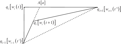
Figure 3: The Euclidean distance covered by a configuration of the string from $q_{i-1}[w_{i-1}(t^{\prime})]$ to $q_{i+1}[w_{i+1}(t^{\prime\prime})]$ via $q_{i}[w_{i}(t+1)]$ is less than the same via $q_{i}[w_{i}(t)]$.

Thus, at any time $t$, after updating a weight $w_{i}(t)$, we have

$\|w_{i-1}(t^{\prime})-w_{i}(t+1)\|+\|w_{i}(t+1)-w_{i+1}(t^{\prime\prime})\|<\\ \|w_{i-1}(t^{\prime})-w_{i}(t)\|+\|w_{i}(t)-w_{i+1}(t^{\prime\prime})\|$

i.e. updating $w_{i}(t)$ contributes to minimization of the sum of lengths of the segments $\overline{q_{i-1}[w_{i-1}(t^{\prime})]q_{i}[w_{i}(t)]}$ and $\overline{q_{i}[w_{i}(t)]q_{i+1}[w_{i+1}(t^{\prime\prime})]}$. Each weight is updated exactly once in every sweep. Thus updating a weight contributes to minimization of length of the current configuration of the string at every sweep, thereby minimizing $\phi(w)$. ∎

Theorem 1 shows the STON algorithm guarantees that the final configuration $\pi_{s}$ of the string belongs to the same homotopy class as its initial configuration $\pi_{i}$. By Theorem 2, it can be seen that if sufficient number of sweeps are computed, the shortest configuration in the given homotopy class can be reached. Thus the proposed algorithm is correct with respect to the goal of obtaining the shortest homotopic configuration of a string as defined in section 2.2. This, however, does not guarantee that the optimum solution will always be reached. It is possible for the algorithm to get stuck at suboptimal solutions, a situation that can be averted by choosing $\alpha$ much less than unity when feature vectors are selected by eq. 3. We shall discuss this issue further in section 5.

4 Computation of shortest homotopic paths

The solution to the problem of computing the shortest homotopic path can be viewed as an instance of pulling a string to tighten it, where the given path corresponds to the initial configuration of the string while the shortest homotopic path corresponds to the tightened configuration of the same string. The STON assumes a string to be sampled such that there exists at most one obstacle in the triangle formed by any three consecutive processors. In this section, given a path $\pi_{i}$, we propose an extension of STON to do away with that assumption and apply the extension for computing the shortest homotopic path $\pi_{s}$ with respect to a given set of obstacles $P$, where $\pi_{i}$ might be simple or non-simple. The set of obstacles $P$ is specified as a set of points in $\Re^{2}$ with no assumption being made about their connectivity. The input path $\pi_{i}$ is specified in terms of a pair of terminal points and either a mathematical equation or a sequence of points in $\Re^{2}$. In the former case, the path is sampled to obtain the sequence of points in $\Re^{2}$.

4.1 Extending STON for sparsely sampled paths

When a path is sampled sparsely, it can no longer be guaranteed that at the time of choosing a feature vector, there will exist only one obstacle within the triangular area spanned by any three consecutive processors. Hence, the algorithm might fail to perform correctly as Theorem 1 no longer holds true (see Fig. 4).

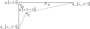
Figure 4: The STON algorithm might fail to perform correctly if the given path is sparsely sampled, as illustrated in the example above. The configuration formed by $q_{i-1}[w_{i-1}(t^{\prime})]$, $q_{i}[w_{i}(t)]$, $q_{i+1}[w_{i+1}(t^{\prime\prime})]$ and that formed by $q_{i-1}[w_{i-1}(t^{\prime})]$, $q_{i}[w_{i}(t+1)]$, $q_{i+1}[w_{i+1}(t^{\prime\prime})]$ are not homotopic to each other as the obstacle $p_{l}$ has been crossed.

Let us assume the given path is very sparsely sampled. In that case, whenever more than one obstacle point is encountered within a triangle formed by three consecutive processors $q_{i-1}$, $q_{i}$, $q_{i+1}$, the centroid, say C, of the obstacle points lying within the triangle is computed. The line segments joining the processors $q_{i-1}$ and $q_{i+1}$ to C partitions the obstacle space within the triangle into two disjoint parts. The convex hull of the obstacle points lying within the partition adjacent to the processor $q_{i}$ is computed (see Fig. 5(a)). A new processor is introduced and initialized near each vertex of the convex hull (see Fig. 5(b)). The indices of all processors and their corresponding weights are updated. The processor $q_{i}$ is considered as ”useless” and is deleted. A similar notion of useless units has been used in [11].

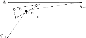
(a) The convex hull of the obstacle points lying in the partition, formed by the line segments joining the processors $q_{i-1}$ and $q_{i+1}$ to C, adjacent to $q_{i}$, is shown.

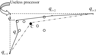
(b) Introduction of new processors $q_{i}$, $q_{i+1}$, $q_{i+2}$ near the vertices of the convex hull.

Figure 5: C is the centroid of all obstacle points lying within the triangle formed by $q_{i-1}$, $q_{i}$, $q_{i+1}$.

We claim, this extension of STON works correctly in all cases. Let us, for a contradiction, assume that there exists an obstacle in the partition not adjacent to the processor $q_{i}$ (see Fig. 5(a)) at which a processor has to be introduced in order to obtain the shortest homotopic path. That is, the shortest homotopic path will pass through an obstacle in the partition not adjacent to the processor $q_{i}$. Let $p_{j}$ be such an obstacle point (see Fig. 6). The line from $q_{i-1}$ through $p_{j}$ partitions the triangle formed by $q_{i-1}$, $q_{i}$, $q_{i+1}$ into two disjoint parts. If the shortest homotopic path passes through $p_{j}$, there cannot exist any obstacle point in the partition, formed by the line from $q_{i-1}$ through $p_{j}$, adjacent to $q_{i}$. But in that case, the centroid C cannot lie in the partition, formed by the line from $q_{i-1}$ through $p_{j}$, adjacent to $q_{i}$. Hence, a contradiction. If the shortest homotopic path passes through $p_{j}$, the centroid C will lie in the partition, formed by the line from $q_{i-1}$ through $p_{j}$, not adjacent to $q_{i}$. In that case, the obstacle point $p_{j}$ lies in the partition, formed by line segments joining processors $q_{i-1}$ and $q_{i+1}$ to C, adjacent to $q_{i}$. Hence the claim follows.

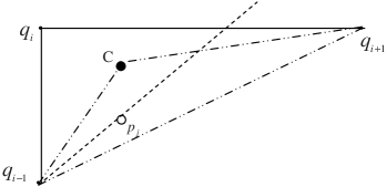
Figure 6: The shortest homotopic path cannot pass through any obstacle point lying in the partition, formed by line segments joining processors $q_{i-1}$ and $q_{i+1}$ to C, not adjacent to $q_{i}$.

4.2 The algorithm: Extension of STON

Input: Set of obstacles, Initial string configuration (i.e. initial sequence of processors)
Output: Final string configuration (i.e. final sequence of processors)
1. initialize the weights
2. $t\leftarrow 0$
3. while convergence criteria (eq. 5) not satisfied, do
4.     $t\leftarrow t+1$
5.     for each processor on path, do
6.        $z\leftarrow$number of obstacles inside triangle formed with neighboring processors
7.        if $z=0$,
8.          create feature vector (eq. 2)
9.          update weight (eq. 4)
10.      if $z=1$,
11.        select feature vector (eq. 3)
12.        update weight (eq. 4)
13.      if $z>1$,
14.        compute convex hull of the selected obstacles
15.        introduce new processors (Appendix A.2) and update their weights (eq. 4)
16. return sequence of processors

First, note that the algorithm for the original version of STON comprised of steps $1$ through $12$ of the above algorithm. Computational complexity of step $6$ is $O(logn+m)$ where $n$ is the number of obstacle points and $m$ is the number of obstacle points inside the triangle formed by a processor and its adjacent neighbors, $0\leq m\leq n$. This complexity can be achieved by a one-time construction of a $2D$ range tree of the obstacle points in $O(nlogn)$ time. Querying the tree requires $O(logn+m)$ time using fractional cascading [31]. On average, $m=\frac{n}{k}$ where $k$ is the number of processors. Thus, complexity of STON is $O(logn+n/k)$ per processor per sweep, assuming the input path has been sampled at half the minimum distance between the obstacles. The purpose of extending STON is to eliminate the constraint on sampling. As a result, steps $13-15$ had to be introduced which uses the algorithm recursively for computing convex hull. Let $T(n)$ be the complexity of extension of STON for each sweep and $k$ be the number of processors at the end of a sweep. Then, from the above algorithm, we get

$$T(n)=k(r_{c}T(m)+logn+m)$$ (6)

where $r_{c}$ is the number of sweeps required to compute convex hull. The convex hull is computed to determine the number and locations of new processors that have to be introduced so that there does not exist more than one obstacle in any triangle formed by three consecutive processors. For this purpose, it is sufficient to compute just one sweep of the convex hull instead of a tight convex hull. This strategy saves computational costs as the newly added processors will eventually not remain on the convex hull of the obstacles but will remain on the path. Therefore,

$$T(n)=k(T(\frac{n}{k})+logn+\frac{n}{k})=O(n(logk+log_{k}n))$$ (7)

Thus the complexity of extension of STON is $O(\frac{n}{k}(logk+log_{k}n))$ per processor per sweep. As the number of processors ($k$) increases, $m\rightarrow 1$, and the complexity of extension of STON becomes $O(logn)$. Thus the extension of STON starts with a complexity of $O(\frac{n}{k}(logk+log_{k}n))$ and reaches a complexity of $O(logn)$ when no more processors are required to be introduced. It is interesting to note that the complexity of STON is comparable with that of some of the recently proposed variants of SOM [10, 32].

In computational geometry, many researchers have proposed algorithms to solve this problem with the primary goal of minimizing computational complexity (refer to [12] for a detailed review). Efrat et al [33] and Bespamyatnikh [34] have independently proposed output sensitive algorithms for the problem. Their algorithms tackle the problem for simple and non-simple paths in different ways, with the one for non-simple paths having higher complexity. Bespamyatnikh’s algorithm for non-simple paths achieves $O(log^{2}n)$ time per output vertex. If the terminal points of a given path are not fixed, the resulting problem is NP-hard [35] which has not been dealt with in this paper.

5 Experimental Results

In this section, we present experimental results obtained by deploying STON to different data sets for different purposes. The extension of STON has been used to compute shortest homotopic paths, smooth paths, and convex hulls. In Fig. 7, the performance of STON is illustrated assuming $\alpha$ is assigned a large value close to unity when feature vectors are chosen according to eq. 3. In that case, the algorithm might fail to perform optimally as the final path might cling to undesired obstacles, as shown by the arrow in Fig. 7. This happens because once a processor falls on an obstacle, which might happen for some processors before convergence if $\alpha$ is large, the processor fails to let the obstacle go as the obstacle continues to remain within its triangle and the processor has no memory of which direction it proceeded from. Such performance from STON can only be averted by choosing $\alpha$ much smaller than unity when feature vectors are selected by eq. 3. This provides ample time for the processors to distribute themselves along the path before coming close to any obstacle. For our experiments, $\alpha$ was chosen as follows

$$\alpha(t)=\left\{\begin{array}[]{ll}1.0&\mbox{if feature vector is created}\\ \beta(1+\frac{t}{T})&\mbox{if feature vector is selected}\end{array}\right.$$ (8)

where $\beta$ is the learning constant, $0<\beta<0.5$, and $T$ is the total number of sweeps that STON is expected to converge within. Typically, $\beta$ and $T$ are assigned values 0.01 and 5000 respectively. Thus, initially a processor proceeds slowly towards the chosen obstacle but the rate of proceeding increases as more and more sweeps are computed. This prevents STON from converging at suboptimal solutions. Throughout our experiments, $\epsilon$ is chosen to be 0.001% of the maximum distance covered along any one dimension by the obstacles.

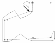
Figure 7: STON works incorrectly for large values of $\alpha$. Circles represent point obstacles, while dark and light lines represent initial and tightened configurations of a path respectively.

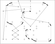
(a) At initialization.

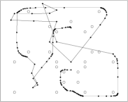
(b) After first sweep.

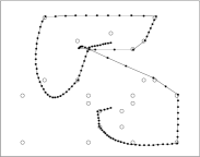
(c) After 5 sweeps.

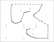
(d) After 10 sweeps.

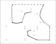
(e) After 15 sweeps.

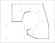
(f) After 20 sweeps.

Figure 8: STON applied to a non-simple path that turns out to be simple when tightened. Circles denote point obstacles while dots denote locations of processors on the path.

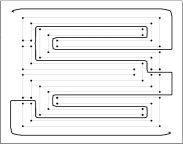
(a) At initialization.

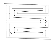
(b) After 15 sweeps.

Figure 9: Performance of STON in a structured obstacle environment. Dotted lines represent the contours of the obstacles while firm lines represent paths.

Fig. 8(a) illustrates a complicated configuration of a path that has not been sampled uniformly. STON was applied to shorten this path and the configurations reached after 1, 5, 10, 15, 20 sweeps are shown in Fig. 8. It can be seen that the processors gradually distribute themselves evenly along the path due to their weights being updated with respect to created feature vectors (eq. 2). This and the assignment of $\alpha$ according to eq. 8 help STON to avoid suboptimal convergence which could have been the case after 10 sweeps (see Fig. 8(d)). The correct shortest configuration was reached within 20 sweeps.

Fig. 9 illustrates the performance of STON in a structured environment where obstacles are not point objects but are two dimensional shapes. The algorithm converged within 15 sweeps. In a structured environment, STON considers the points forming the two dimensional shapes as point obstacles and does not use their connectivity information. The algorithm performs equally well in structured as well as unstructured environments.

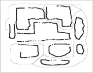
(a) At initialization.

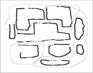
(b) After first sweep.

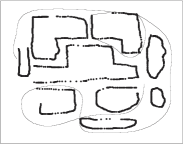
(c) After 10 sweeps.

(d) After 20 sweeps.

Figure 10: STON finds a smooth homotopic path with respect to a huge set (thousands) of obstacles. Dots represent point obstacles while firm lines represent paths.

In real world applications, such as navigational planning of mobile robots [26] or route formation for military planning [14, 15, 19, 21, 24], the absolute shortest path is not always desired; a suboptimal path that is devoid of sharp turns is often more desirable in such cases. Fig. 10 shows the capability of STON to produce such paths by appropriately adjusting the parameter $\epsilon$. In this case, $\epsilon$ was chosen to be 0.1%. The illustration in Fig. 10 further demonstrates the capability of STON to handle a huge number of obstacles, in the range of a few thousand.

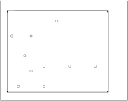
(a) At initialization.

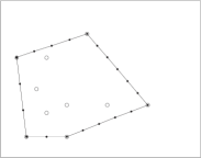
(b) After 10 sweeps.

Figure 11: STON computes the convex hull of a set of points represented by circles. Lines represent the contour of the convex hull while dots on the contour represent locations of the processors.

STON can be used to compute the convex hull of a set of points, as shown in Fig. 11. A path has a starting and an ending point which are fixed and common for all paths belonging to the same homotopy class. To exploit this information for computation of shortest homotopic paths, the first and the last processors, $q_{1}$ and $q_{k}$, on a path with $k$ processors were assumed to be fixed and their corresponding weights were never updated. Computation of convex hull however does not require any fixed processors, so weights corresponding to all processors were updated. The starting and ending points were assumed to be the same. Such a modification of STON makes it functionally similar to an elastic band or a Snake [36].

Experiments with a number of different data sets, a few of which are shown in Fig. 7 through 11, assuming the learning constant $\beta$ to be $10^{-2}$, reveal certain characteristics of STON. It is expected that the total number of sweeps required for convergence increases with the increase in number of processors. Outcomes of our experiments satisfy such expectations but they also show that average number of sweeps per processor required for convergence decreases with the increase in number of processors (see Fig. 12). This is important in determining how many processors to sample a path with as one should choose the optimum number of processors for minimizing computational costs. The errors in Fig. 12 refer to the ratio of the length of the shortened path at convergence with respect to the length of the shortest path.

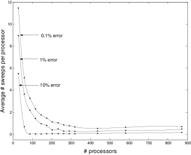
Figure 12: Experiments show that average number of sweeps per processor required for convergence using STON decreases with the increase in number of processors.

The learning rate is an important factor for ensuring faster convergence. The number of processors being fixed, total number of sweeps required for convergence increases with decrease in learning constant $\beta$ (see Fig. 13). We experimented with a number of data sets including those shown in Fig. 7 through 11, sampling the paths with 30, 59, 88, 117, 146, 175 processors at different locations and varying the learning constant $\beta$ from $10^{-4}$ to 0.2 for each data set. Choosing a very high learning constant might lead to suboptimal results as has been illustrated in Fig. 7. It is interesting to note from Fig. 13 that for low learning constants, such as $10^{-2}$ or lesser, the total number of sweeps required for convergence is more for lesser number of processors. This observation only reinforces the fact that average number of sweeps per processor decreases with the increase in number of processors for low learning constants.

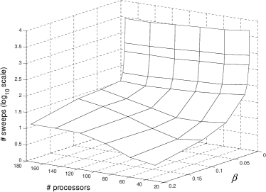
Figure 13: As the learning constant decreases, the number of sweeps required for convergence using STON increases.

6 Conclusion

A self-organizing neural network algorithm STON is proposed that models the phenomenon undergone by the particles forming a string when the string is tightened from one or both of its ends amidst obstacles. Discussions of the properties and correctness of this anytime algorithm is presented assuming the given string is sampled at a frequency of at least $d/2$ where $d$ is the minimum distance between the obstacles. It is shown how STON might be extended for tightening strings when the above constraint on sampling is not met. This extension is applied to compute the shortest homotopic path with respect to a set of obstacles. Proof of correctness and computational complexity of the extension of STON are included. Experimental results show that the proposed algorithm works correctly with both simple and non-simple paths in reasonable time as long as the constraints for correctness are met. STON is used to generate smooth and shorter homotopic paths, a problem that can be modeled as the phenomenon of tightening a string. STON is also used as an elastic band for computing convex hulls. Future research aims at improving the computational complexity of the extension of STON and using it to solve more problems that can be mapped into the problem of tightening a string or an elastic band.

Appendix A Appendices

A.1 A Finite Sampling Theorem

A string in $\Re^{2}$, wound around point obstacles, can be finitely sampled in such a way so as to guarantee only one obstacle within the triangular area spanned by any three consecutive points on the string. The following theorem states the constraint necessary to be imposed on the sampling.

Theorem 3.

Sampling a string at half the minimum distance between the obstacles guarantees at most one obstacle in any triangle formed by three consecutive points on the string.

Proof.

Let $d$ be the minimum distance between any two unique obstacles in $P$, $P$ being the set of point obstacles. Let us sample the string such that the distance between any two consecutive points on the string is at most $d/2$. Since $d$ is finite, clearly this leads to a finite sampling of the string. The theorem claims, this sampling ensures that a triangle formed by any three consecutive points on the string will never contain more than one unique obstacle.

For contradiction, let us assume, there exists two obstacle points in a triangle formed by three consecutive points $q_{i-1}$, $q_{i}$, $q_{i+1}$ (see Fig. 14). The segments $\overline{q_{i-1}q_{i}}$ and $\overline{q_{i}q_{i+1}}$ included in the string that form two sides of the triangle are each of length at most $d/2$. Thus the maximum distance between any two points lying within the triangle is less than $d$. But the distance between any two obstacle points is at least $d$. Hence, a contradiction, and the claim follows. ∎

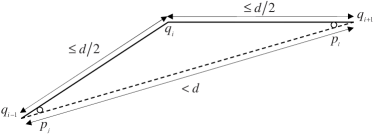
Figure 14: Sampling a path uniformly at half the minimum distance between the obstacles guarantees at most one obstacle in any triangle.

A.2 Procedure for Introducing Processors in Convex Hull

Here we describe the procedure for introducing processors near each vertex of the convex hull in the extension of STON. The newly introduced processor, say $q_{i}$, should be placed at a location such that connecting it with the neighboring processors, $q_{i-1}$ and $q_{i+1}$, does not alter the homotopy class of the path i.e. the path in which the new processors are being introduced should remain in the same homotopy class as the given path. This is not a trivial task as illustrated in Fig. 15, where all the processors are introduced near the convex hull but the new path $\pi_{new}$ is not homotopic to the old path $\pi_{old}$.

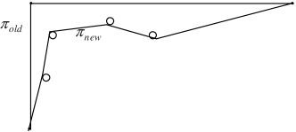
Figure 15: Introducing processors anywhere near the vertices (shown by circles) of the convex hull does not guarantee the new path will be homotopic to the old one.

In order for the new path to remain in the same homotopy class as the old one, processors cannot be introduced within the convex hull and lines joining consecutive processors cannot intersect the edges of the convex hull.

Theorem 4.

If processors are introduced outside the convex hull in the regions bounded by the extended adjacent edges of the convex hull, then the lines joining the consecutive processors will not intersect the edges of the convex hull.

Proof.

Let $V_{1}V_{2}V_{3}...V_{m}$ be a $m$-sided polygon which is the convex hull for a set of obstacles under consideration (see Fig. 16). Let $q_{i}$ be a processor in the region formed by extensions of adjacent edges $\overline{V_{i-1}V_{i}}$ and $\overline{V_{i+1}V_{i}}$, $\forall i$, $1\leq i\leq m$. The claim states that there cannot be an intersection between the line segment $\overline{q_{j}q_{j+1}}$ and any edge of the convex hull.

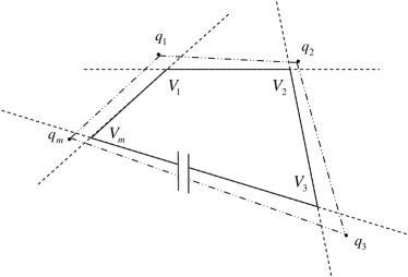
Figure 16: Introduction of processors outside the convex hull in the regions bounded by the extended adjacent edges of the convex hull guarantees that the lines joining the consecutive processors will not intersect the edges of the convex hull.

Let us assume, for a contradiction, there exists at least one intersection between the line segment $\overline{q_{j}q_{j+1}}$ and an edge, say $\overline{V_{k}V_{k+1}}$, of the convex polygon $V_{1}V_{2}V_{3}...V_{m}$. Then, $q_{j}$ and $q_{j+1}$ must lie on the opposite sides of the extended line segment $\overline{V_{j}V_{j+1}}$. But by construction, the processors $q_{j}$, $q_{j+1}$ lie on the same side of the extended line segment $\overline{V_{j}V_{j+1}}$. Hence a contradiction and the claim follows. ∎

References

- [1] B. Banerjee. String tightening as a self-organizing phenomenon. IEEE Trans. Neural Networks, 18(5):1463–1471, 2007.
- [2] T. Kohonen. Self-Organizing Maps. Springer, Berlin, 2001.
- [3] J.A. Kangas, T. Kohonen, and J. Laaksonen. Variants of self-organizing maps. IEEE Trans. Neural Networks, 1:93–99, 1990.
- [4] B. Fritzke. Growing cell structures - a self-organizing network for unsupervised and supervised learning. Neural Networks, 7(9):1441–1460, 1994.
- [5] D. Choi and S. Park. Self-creating and organizing neural networks. IEEE Trans. Neural Networks, 5(4):561–575, 1994.
- [6] L. Schweizer, G. Parladori, L. Sicuranza, and S. Marsi. A fully neural approach to image compression. In T. Kohonen, K. Makisara, O. Simula, and J. Kangas, editors, Artificial Neural Networks, pages 815–820, North-Holland, Amsterdam, 1991.
- [7] K. Obermayer, H. Ritter, and K. Schulten. Large-scale simulations of self-organizing neural networks on parallel computers: application to biological modeling. Parallel Computing, 14:381–404, 1990.
- [8] F. Favata and R. Walker. A study of the application of Kohonen-type neural networks to the traveling salesman problem. Biol. Cybernetics, 64:463–468, 1991.
- [9] H. J. Ritter and T. Kohonen. Self-organizing semantic maps. Biol. Cybernetics, 61:241–254, 1989.
- [10] H. Kusumoto and Y. Takefuji. self-organizing map algorithm without learning of neighborhood vectors. IEEE Trans. Neural Networks, 17(6):1656–1661, 2006.
- [11] B. Fritzke. A self-organizing network that can follow non-stationary distributions. In Proc. Intl. Conf. Artificial Neural Networks, pages 613–618. Springer, 1997.
- [12] J. S. B. Mitchell. Geometric shortest paths and network optimization. In J. R. Sack and J. Urrutia, editors, Handbook on Computational Geometry, pages 633–702. Elsevier Science, 2000.
- [13] H. Choset, K. Lynch, S. Hutchinson, G. Kantor, W. Burgard, L. Kavraki, and S. Thrun. Principles of Robot Motion: Theory, Algorithms, and Implementation. MIT Press, Cambridge, 2005.
- [14] B. Chandrasekaran, J. R. Josephson, B. Banerjee, U. Kurup, and R. Winkler. Diagrammatic reasoning in support of situation understanding and planning. In Proc. 23rd Army Sci. Conf., Orlando, FL, 2002.
- [15] B. Banerjee, B. Chandrasekaran, J. R. Josephson, and R. Winkler. Constructing diagrams to support situation understanding and planning: Part 1: Diagramming group motions. Technical report, Ohio State University, Columbus, 2003.
- [16] B. Chandrasekaran, U. Kurup, B. Banerjee, J. R. Josephson, and R. Winkler. An architecture for problem solving with diagrams. In A. Blackwell, K. Marriott, and A. Shimojima, editors, Lecture Notes in AI, volume 2980, pages 151–165. Springer-Verlag, 2004.
- [17] B. Chandrasekaran, U. Kurup, and B. Banerjee. A diagrammatic reasoning architecture: Design, implementation and experiments. In Proc. AAAI Spring Symp., Reasoning with Mental and External Diagrams: Computational Modeling and Spatial Assistance, pages 108–113, Stanford University, CA, 2005.
- [18] B. Banerjee. A layered abductive inference framework for diagramming group motions. Special Issue of Logic J. IGPL: Abduction, Practical Reasoning, and Creative Inferences in Sci., 14(2):363–378, 2006.
- [19] B. Banerjee and B. Chandrasekaran. A framework for planning multiple paths in free space. In Proc. 25th Army Sci. Conf., Orlando, FL, 2006.
- [20] B. Banerjee. Spatial problem solving for diagrammatic reasoning. PhD thesis, Dept. of Computer Science & Engineering, The Ohio State University, Columbus, 2007.
- [21] B. Chandrasekaran, B. Banerjee, U. Kurup, J. R. Josephson, and R. Winkler. Diagrammatic reasoning in army situation understanding and planning: Architecture for decision support and cognitive modeling. In P. McDermott and L. Allender, editors, Advanced Decision Architectures for the Warfighter: Foundations and Technology, chapter 21, pages 379–394. 2009.
- [22] B. Banerjee and B. Chandrasekaran. A spatial search framework for executing perceptions and actions in diagrammatic reasoning. In Lecture Notes in AI, volume 6170, pages 144–159. Springer, Heidelberg, 2010.
- [23] B. Banerjee and B. Chandrasekaran. A constraint satisfaction framework for executing perceptions and actions in diagrammatic reasoning. Journal of Artificial Intelligence Research, 39:373–427, 2010.
- [24] B. Banerjee and B. Chandrasekaran. A framework of voronoi diagram for planning multiple paths in free space. Journal of Experimental & Theoretical Artificial Intelligence, 25(4):457–475, 2012.
- [25] S. Gao, M. Jerrum, M. Kaufmann, K. Mehlhorn, and W. R lling. On continuous homotopic one layer routing. In Proc. Symp. Comput. Geometry, pages 392–402, 1988.
- [26] S. Quinlan and O. Khatib. Elastic bands: connecting path planning and robot control. In Proc. IEEE Intl. Conf. Robotics and Automation, volume 2, pages 802–807, Atlanta, GA, 1993.
- [27] D. Grigoriev and A. Slissenko. Polytime algorithm for the shortest path in a homotopy class amidst semi-algebraic obstacles in the plane. In Proc. Intl. Symp. Symbolic and Algebraic Computation, pages 17–24, Rostock, Germany, 1998.
- [28] F. Rosenblatt. The perceptron: a probabilistic model for information storage and organization in the brain. Psychological Review, 65(6):386–408, 1958.
- [29] E. Berglund and J. Sitte. The parameterless self-organizing map algorithm. IEEE Trans. Neural Networks, 17(2):305–316, 2006.
- [30] T. De Wolf and T. Holvoet. Emergence versus self-organisation: different concepts but promising when combined. Engineering Self Organising Systems: Methodologies and Applications, Lecture Notes in Computer Sci., 3464:1–15, 2005.
- [31] M. de Berg, M. van Kreveld, M. Overmars, and O. Schwarzkopf. Computational Geometry. Springer-Verlag, 1997.
- [32] S. Pal, A. Datta, and N. R. Pal. A multilayer self-organizing model for convex-hull computation. IEEE Trans. Neural Networks, 12(6):1341–1347, 2001.
- [33] A. Efrat, S. G. Kobourov, and A. Lubiw. Computing homotopic shortest paths efficiently. In Proc. 10th Annual European Symp. Comput. Geometry, pages 411–423, 2002.
- [34] S. Bespamyatnikh. Computing homotopic shortest paths in the plane. J. Algorithms, 49(2):284–303, 2003.
- [35] D. Richards. Complexity of single-layer routing. IEEE Trans. Computers, 33(3):286–288, 1984.
- [36] M. Kass, A. Witkin, and D. Terzopoulos. Snakes active contour models. Intl. J. Computer Vision, pages 321–331, 1988.