Spectral and polarization properties of black hole accretion disc emission: including absorption effects

Abstract

The study of radiation emitted from black hole accretion discs represents a crucial way to understand the main physical properties of these sources, and in particular the black hole spin. Beside spectral analysis, polarimetry is becoming more and more important, motivated by the development of new techniques which will soon allow to perform measurements also in the X- and $\gamma$-rays. Photons emitted from black hole accretion discs in the soft state are indeed expected to be polarized, with an energy dependence which can provide an estimate of the black hole spin. Calculations performed so far, however, considered scattering as the only process to determine the polarization state of the emitted radiation, implicitly assuming that the temperatures involved are such that material in the disc is entirely ionized. In this work we generalize the problem by calculating the ionization structure of a surface layer of the disc with the public code cloudy, and then by determining the polarization properties of the emerging radiation using the Monte Carlo code stokes. This allows us to account for absorption effects alongside scattering ones. We show that including absorption can deeply modify the polarization properties of the emerging radiation with respect to what is obtained in the pure-scattering limit. As a general rule, we find that the polarization degree is larger when absorption is more important, which occurs e.g. for low accretion rates and/or spins when the ionization of the matter in the innermost accretion disc regions is far from complete.

1 Introduction

The black hole spin in accreting stellar-mass black hole binary systems is currently estimated by using spectroscopic (either the iron $K\alpha$ line profile or the thermal disc continuum emission) or timing (kHz QPOs) techniques (see Reynolds, 2019, and references therein). A fourth technique, based on the energy dependence of the polarization degree and angle of the thermal disc emission, has been proposed in the late 70s Connors & Stark (1977); Stark & Connors (1977); Connors, Piran & Stark (1980), and then revisited more recently Dovčiak et al. (2008); Li, Narayan & McClintock (2009); Schnittman & Krolik (2009); Taverna et al. (2020). The renewed interest in the polarimetric technique is due to, on one hand, the discrepant results provided by the other techniques in a few cases (most notably GRO J1655-40, Motta et al., 2014) and, on the other hand, to the re-opening of the X-ray polarimetric observing window provided by missions like IXPE Weisskopf et al. (2013), due to be launched in 2021, and on a more distant future by eXTP Zhang et al. (2019).

This technique is based on the influence of strong gravity on the polarization degree and angle of radiation. The polarization angle, in particular, is expected to rotate along the geodesics; the rotation is larger for more energetic photons, because they are mostly emitted closer to the black hole. When convolving over the entire disc emission, an energy dependence of the polarization angle results. This effect is larger the larger the spin of the black hole (because of the lower value of the Innermost Stable Circular Orbit, ISCO), which can therefore be determined (see in particular Dovčiak et al., 2008).

Schnittman & Krolik (2009) included in their analysis the contribution of returning radiation, i.e. photons that, following null geodesics in the space-time around the BH, return to the disc before being reflected (in the hypothesis of $100\%$ albedo) towards the observer. They showed that spectra and polarization observables can be deeply modified with respect to those of direct radiation only due to the effects of reflection at the disc surface. Taverna et al. (2020) investigated the effects of considering different scattering optical depths on the intrinsic polarization and calculated how the spectra and polarization observables of both direct and returning radiation are modified when a more realistic albedo profile is used to characterize the disc surface.

In all the previous works, however, the polarization of the thermal disc is either calculated assuming a pure scattering slab of material Dovčiak et al. (2008) or the Chandrasekhar’s (1960) prescription, valid for a plane-parallel, semi-infinite scattering atmosphere. To date, a self-consistent treatment for studying spectral and polarization properties of stellar-mass BH accretion disc emission accounting for absorption effects alongside scattering ones is still lacking, although the method described in Taverna et al. (2020) to include a more realistic albedo profile for the disc surface can be considered as a first attempt in this direction.

In the present work we still adopt the scenario of a thermal disc covered by a surface atmosphere, as in previous ones. Here, however, we move a further step forward by including in the polarized radiative transfer calculations absorption effects in the partially-ionized slab material. To this aim, we first model the ionization structure of an optically-thick, surface layer of the disc using the photo-ionization code cloudy Ferland et al. (2017). Secondly, we solve the radiative transfer for photons propagating within this surface layer, exploiting the Monte Carlo code stokes (Marin, 2018, see also Goosmann & Gaskell 2007). While our physical assumption of an ionized slab above a black body emitting disc is certainly simplistic, it allows us to start addressing the issue of the effect of absorption on the polarization properties of the emerging radiation. A self-consistent, simultaneous treatment of the disc structure and of polarized radiative transfer is beyond the scope of the present paper. Spectra and polarization properties are provided at the source, without considering the general relativistic corrections that affect the photon transport to the observer; the complete description of photon spectra and polarization as they would be measured at infinity will be handled in a future publication.

The plan of the paper is as follows: in section 2 we recall the general concepts of our theoretical model, and describe in more details the numerical implementation in section 3. Results and comparisons with previous works are introduced in section 4. Finally, we summarize our findings and present our conclusions in section 5.

2 The model

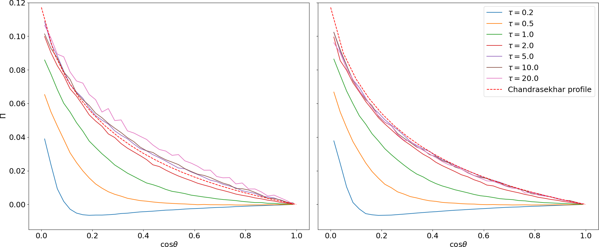
Figure 1: Polarization degree in the pure-scattering limit, plotted as a function of the cosine of the inclination angle $\theta$ for isotropic emission from the bottom of the disc surface slab. Positive values correspond to polarization parallel to the disc plane ($\chi=0^{\circ}$), while negative ones to polarization in the direction of the disc axis ($\chi=90^{\circ}$). Different values of the Thomson optical depth $\tau$ are explored: $0.2$ (cyan), $0.5$ (orange), $1$ (green), $2$ (magenta), $5$ (purple), $10$ (brown) and $20$ (pink). The polarization degree angular profile as described in Chandrasekhar (1960, see Table XXIV) is also shown for comparison (red-dashed line). Stokes parameters have been summed over the $2$–$8$ keV (left-hand panel) and the $0.5$–$20$ keV (right-hand panel) energy bands.

We recall in this section our basic assumptions. As described in previous works (see e.g. Taverna et al., 2020; Dovčiak et al., 2008), we consider the accretion disc as a standard disc (see Shakura & Sunayev, 1973), with particles rotating around the center at the Keplerian velocity. The central, stellar mass BH is characterized by the values of its mass $M$ and dimensionless angular momentum $a$, with the space-time around described by the Kerr metric Novikov & Thorne (1973). The disc stops at the radius of the ISCO $r_{\rm ms}$ (see Bardeen et al., 1972), and no-torque at the inner boundary is assumed.

Internal viscous dissipations heat up the surface layers of the disc. We handle the distribution of the emitted photons through a local blackbody, with the temperature $T$ varying with the radial distance $r$ from the center according to the Novikov-Thorne profile Novikov & Thorne (1973),

$$T(\xi,M,\dot{M},a) =741f_{\rm col}\left(\frac{M}{\rm M_{\odot}}\right)^{-1/2}\left(\frac{\dot{M}}{\rm M_{\odot}\,yr^{-1}}\right)^{1/4}$$

$$\,\,\,\,\,\,\times[f(\xi,a)]^{1/4}\,{\rm keV}\,;$$ (1)

here $\xi=(r/r_{\rm g})^{1/2}$ (with $r_{\rm g}=GM/c^{2}$ the gravitational radius), $\dot{M}$ is the BH accretion rate and $f$ is a function of $\xi$ and the BH spin $a$ (see Taverna et al., 2020, for the complete expression; see also Page & Thorne 1974; Wang 2000). In equation (2) we account for the energy shift of photons due to the scatterings they undergo with particles in the deepest layers of the disc through the hardening factor $f_{\rm col}$ Shimura & Takahara (1995); Dovčiak et al. (2008); Davis & El-Abd (2019).

The density of the disc material is modelled according to the radial profile discussed by Compère & Oliveri (2017), who provide the expressions for the total (hydrogen) density $n_{0}(\rm H)$ at the equatorial plane (see Taverna et al., 2020, for more details). For ease of reading we reported the main formulae in Appendix A. In order to obtain the corresponding values of the density at the disc surface, we assume for the sake of simplicity a Gaussian prescription for the vertical structure, so that

$$n({\rm H},z_{*}) =n_{0}({\rm H})\exp\left(-\frac{z_{*}^{2}(r)}{h^{2}}\right)\,,$$ (2)

where $h$ is the typical height of the disc at the radial distance $r$ and $z_{*}$ is the altitude above the disc equatorial plane at which the scattering optical depth calculated up to infinity is equal to 1 Taverna et al. (2020).

We solve the ionization structure of the disc only in its surface layer, in which the emitted blackbody radiation is processed. To describe the matter that composes this layer, we adopted the typical solar abundance Asplund et al. (2005), focussing in particular on the elements with $Z=1$ (hydrogen), $2$ (helium), $6$ (carbon), $7$ (nitrogen), $8$ (oxygen), $10$ (neon), $14$ (silicon), $16$ (sulfur) and $26$ (iron), neglecting the presence of dust.

3 Numerical implementation

In order to reproduce both the spectral and polarization properties of the radiation emerging from the accretion disc, we use the Monte Carlo code stokes (Marin, 2018, see also Marin et al. 2012; Goosmann & Gaskell 2007). This code was originally developed to solve the radiative transfer of near-IR to UV photons propagating inside regions of material where scattering represents the main source of opacity (like e.g. in AGN). However, with the purpose of adapting the code to our case, we resorted to the upgraded version 2.33 of stokes, optimized for modeling the X-ray radiation propagating through a stratified, plane-parallel atmosphere, which fully adapts to describe the surface layer of the disc according to our model. In order to solve the atomic structure in this atmospheric layer, we use the version 17.01 of cloudy (last described in Ferland et al., 2017), an open-source, photo-ionization code to simulate the relevant processes that occur in astrophysical clouds. In particular, since we restrict our investigation to the case in which collisions are the dominant process for ionizing matter, we used the coronal model, which allows us to calculate the ionization properties of a material slab by specifying only the (kinetic) temperature and the total (hydrogen) density of the gas.

The surface atmospheric layer is, then, divided into a number $N_{\rm r}$ of patches, each one at a different radial distance $r$ from the central BH. For the sake of simplicity, we associate to each radial patch the corresponding values of temperature and density at the disc surface, as provided by equations (2) and (• ‣ A)–(• ‣ A), respectively, and we consider them as constant within the same patch. After having defined an $xyz$ reference frame, with the $z$-axis chosen along the disc symmetry axis, the code solves the ionization structure inside the patch by dividing it into several slices, characterized by the height $z$ with respect to the base of the surface layer. The maximum height $z_{\rm max}$ that the code reaches in each run is univocally determined by the input parameter $N_{\rm H}^{\rm stop}$, i.e. the hydrogen column density at which calculations are stopped. For every radial distance $r$ and altitude $z$, we finally extract, from the code output, the fractional abundance of each element in different states of ionization,

$$F^{\rm(i)}_{\rm X^{\alpha}} =\frac{n^{\rm(i)}_{\rm X^{\alpha}}}{n^{\rm tot}_{\rm X}}\,.$$ (3)

In equation (3), $n^{\rm(i)}_{\rm X^{\alpha}}$ is the number density of the ionic species $X^{\alpha}(i)$, with $\alpha$ the ionic charge and $i$ the excitation level of the outermost electron, while $n^{\rm tot}_{\rm X}$ denotes the total number density of the element $X$.

The output of cloudy obtained for each single radial patch is hence processed by a specific c++ script, in order to produce a suitable input file for stokes, containing all the relevant information about the ionization structure. The emission region, from which photons are injected inside the layer can be featured as well in this input file, choosing between different geometries of emission. For our simulations we assumed the emitting source to be located at the bottom of the atmospheric layer ($z=0$); no bulk motion is considered for the emission region. Following our model prescriptions (see §2), for each radial patch of the surface layer we imposed that all the seed photons are emitted according to an isotropic blackbody at the temperature $T(r)$ (see equation 2). This is tantamount to say that the propagation directions, along which photons are launched, are sampled by the polar angles

$$\theta_{\rm e} =\arccos(\sqrt{r_{1}})$$

$$\phi_{\rm e} =2\pi r_{2}$$ (4)

with respect to the $z$-axis and the $xz$-plane, respectively; in equation (3) $r_{1}$ and $r_{2}$ are uniform deviates between $0$ and $1$. Seed radiation is set as unpolarized, i.e. the photon Stokes vectors are initialized to

$$\left(\begin{array}[]{c}i_{0}\\ q_{0}\\ u_{0}\\ v_{0}\end{array}\right) =\left(\begin{array}[]{c}1\\ 0\\ 0\\ 0\end{array}\right)\,.$$ (13)

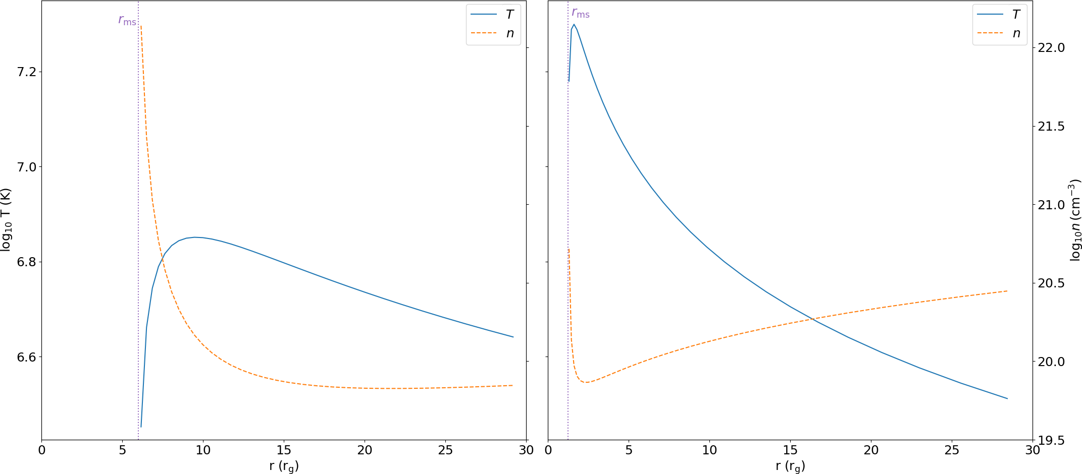
Figure 2: Surface temperature (blue, solid line) and density (orange, dashed line) radial profiles obtained according to equations (2) and (• ‣ A)–(• ‣ A), respectively, in the case of a non-rotating (left-hand panel) and a maximally-rotating (right-hand panel) BH with mass $M=10\,{\rm M}_{\odot}$ and accretion rate $\dot{M}=0.1\,\dot{M}_{\rm Edd}$. The hardening factor $f_{\rm col}$ is set to $1.8$.

Photons are, then, followed along their trajectory, accounting for all the possible interactions (such as multiple scattering, free-free interactions or photoelectric absorptions) they can experience in the surface layer. All the photons which are not absorbed inside the layer are eventually collected in different virtual detectors, each one identified by the inclination $\theta$ and the azimuth $\phi$ which characterize the corresponding viewing direction in the $xyz$ frame. The total number of virtual detectors is fixed by specifying in input the numbers of points $N_{\theta}$ and $N_{\phi}$ of the $(\theta,\phi)$ angular mesh. For each detector, the Stokes parameters of the photons collected along the corresponding viewing direction are summed together, after having rotated the different Stokes parameter reference frames around the detector line-of-sight, to match with the detector frame. The final output of each run (corresponding to each radial distance $r$) consists of the Stokes parameters $i$, $q$, $u$ and $v$ of the emerging radiation as functions of the photon energy $E$ and of the two viewing angles $\theta$ and $\phi$. Given the axial symmetry of the adopted geometry, we actually integrated over $\phi$. The resolution $N_{\rm E}$ and the boundaries $E_{\mathrm{min}}$–$E_{\mathrm{max}}$ of the photon energy band, as well as the number $N_{\rm phot}$ of seed photons to be launched in each single run, can be defined at the beginning of the stokes input file. The linear polarization fraction $\Pi$ and the polarization angle $\chi$ are eventually obtained through the usual expressions

$$\Pi =\frac{\sqrt{q^{2}+u^{2}}}{i}$$

$$\chi =\frac{1}{2}\arctan\left(\frac{u}{q}\right)\,,$$ (14)

where $\chi=0$ corresponds to polarization vectors oriented as perpendicular to the $z$ axis (i.e. lying in the plane of the disc), increasing in the clockwise direction.

Figure 3: Emerging spectra (top row) and polarization degree (bottom row) plotted for the two cases $a=0$ (left-hand column) and $a=0.998$ (right-hand column) and for $\theta=12.8^{\circ}$ (cyan), $39.2^{\circ}$ (orange), $54.9^{\circ}$ (green), $68.0^{\circ}$ (red) and $79.9^{\circ}$ (purple). Here $M=10\,{\rm M}_{\odot}$, $L=0.1\,L_{\rm Edd}$, $N_{\rm H}^{\rm stop}=10^{24}$ cm^-2 and $f_{\rm col}=1.8$. Stokes parameters, weighted for the area and the temperature of each radial patch, are summed over the radial distance $r$ (see equations 4.2).

Finally, it should be noted that, by construction, at each radius the polarization is calculated by stokes assuming a slab with constant density and temperature which is indefinite in the $xy$-plane. As we are dealing with a geometrically thin accretion disc solution, we consider this approximation, which simplifies significantly our computations, as acceptable.

4 Results

In this section we present the results of some significant simulations performed exploiting the codes illustrated in section 3. For the sake of comparison with previous works, we start discussing the outputs obtained from stokes in the pure-scattering limit and then we continue considering the effects of ionization in the disc surface layer. In the following, the angular dependence is resolved in the colatitude $\theta$, while data are summed over the azimuthal angle ($N_{\phi}=1$).

4.1 Pure-scattering limit

The behavior of the polarization degree, after switching-off all interaction processes apart Compton scattering, is shown in Figure 1 as a function of the cosine of the inclination angle $\theta$ (sampled over a $40$-point grid), for different values of the (Thomson) optical depth $\tau$. For each value of $\tau$, $N_{\rm phot}=10^{9}$ photons are injected in the layer according to a blackbody distribution at the temperature $T=1$ keV. Positive values refer to polarization in the plane of the disc ($\chi=0^{\circ}$), while negative ones to perpendicular polarization ($\chi=90^{\circ}$). In the left-hand plot Stokes parameters have been integrated in the $2$–$8$ keV energy band, since this is the typical range of operations of the new-generation X-ray polarimeters like IXPE. In the right-hand one, instead, the $0.5$–$20$ keV band has been considered, as the best compromise between the choice of an energy range in which all the photons are included and the need of a reasonable computational time.

The curves are obtained following the prescriptions discussed in §3, i.e. assuming that photons are emitted isotropically from a pointlike source placed at the bottom of the atmospheric layer, which is a semi-infinite, plane-parallel slab. In almost all the cases explored, polarization vectors turn out to be oriented as parallel to the plane of the disc ($\Pi\ga 0$), with the maximum polarization degree attained at high inclinations and monotonically decreasing down to $\sim 0$ at smaller ones. The only exception occurs at small optical depths ($\tau\la 0.5$), for which polarization may become perpendicular to the disc plane at small inclination angles. In particular, $\Pi$ assumes negative values for $\theta\la 53^{\circ}$ when $\tau=0.5$, while polarization vectors are definitely oriented in the direction of the projected disc symmetry axis for practically the entire range of inclinations for $\tau=0.2$. The effect can be explained as follows. When small values of $\tau$ are considered, photons which are more likely to be scattered are those emitted at large inclinations with respect to the slab normal, since they experience a larger effective optical depth. Because the electric vector of the scattered photons oscillates perpendicularly to the scattering plane, these photons will emerge with orthogonal polarization. On the other hand, photons originally emitted at small inclinations will be practically unpolarized if they emerge at small inclinations too, while, for symmetry reasons, their polarization is expected to be very large and oriented in the plane of the disc if they emerge at large inclinations. As a result, polarization turns out to be negative for a large interval of inclinations, becoming positive only close to $\cos\theta\sim 0$. On the other hand, at large optical depths multiple scattterings can occur, which mitigate this behavior; moreover, scatterings become more and more frequent also for photons emitted at small inclinations, which contribute much more to the overall polarization pattern. The emergence of negative polarization has been originally noted by Nagirner (1962) and Gnedin & Silant’ev (1978), albeit in a slightly different scenario. In particular, the latter authors showed that, while only positive polarization is present if the photons are preferentially emitted deep in an accretion disc, negative polarization arises when the source function is almost constant along the disc vertical structure. In the latter case, as Gnedin & Silant’ev (1978) explain, many photons before the last scattering travel almost parallel to the disc surface, and moreover their scattering angle is close to 90^∘, a situation similar to ours in the case of small optical depths.

Increasing the layer optical depth, the angular behavior of the polarization fraction approaches, as expected, the classic solution obtained by Chandrasekhar (1960) assuming a semi-infinite slab (red-dashed line). In this condition, photons can emerge from the upper boundary of the layer only after a large number of scatterings, at variance with what happens for small optical depths, when a significant number of photons can escape even without suffering any scattering (and then remaining unpolarized). It is interesting to note that the polarization degree attained for optical depths larger than $\sim 5$ turns out to even slightly exceed that expected according to the Chandrasekhar’s profile, as it can be seen looking at the left-hand panel in Figure 1. The reason is that, while the Chandrasekhar’s solution is obtained assuming elastic (Thomson) scattering, in our stokes model Compton downscattering is accounted for. As a consequence of the energy shift toward lower energies, a certain number of photons drops out of the selected energy band, an effect of course increasing with the average number of scatterings (and then with $\tau$). Since the photons that are lost in this way are those which have suffered more interactions, and therefore are more isotropised and less polarized, an increase of $\Pi$ with respect to Chandrasekhar (1960) can be observed when the energy band is restricted to the $2$–$8$ keV range. Results closer to those given by the Chandrasekhar’s solution can be obtained, in fact, by considering a wider energy range, as shown in the right-hand panel of Figure 1, where Stokes parameters are integrated over the $0.5$–$20$ keV band.

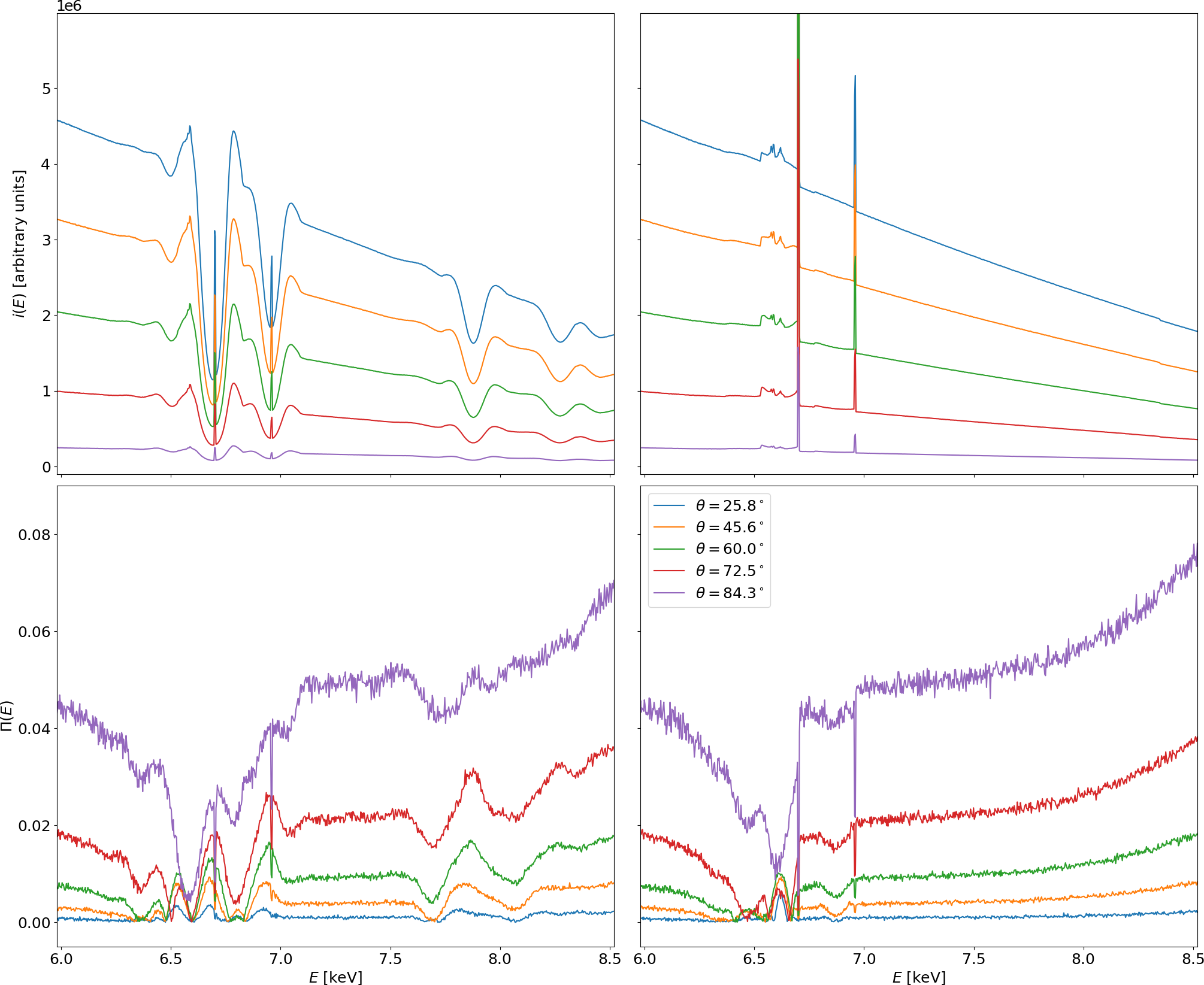
Figure 4: Photon flux (top row) and polarization degree (bottom row) plotted as functions of the photon energy (sampled with a 5000-point grid) in the case of $a=0.998$, for the first radial bin of the disc surface and for five different inclinations of the viewing direction. The values of the other parameters are the same as in Figure 3. Scattering, free-free, recombination and photo-electric absorption effects are accounted for in the plots of the left column, while resonant scattering lines are artificially turned off in those of the right one.

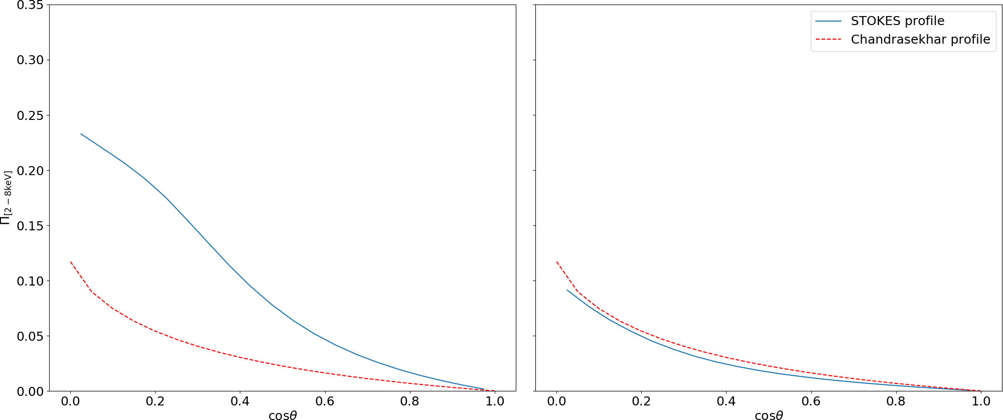
Figure 5: Polarization degree plotted as a function of the cosine of the inclination angle $\theta$ for the two cases of $a=0$ (left-hand panel) and $a=0.998$ (right-hand panel) and the same values of parameters as in Figure 3. Stokes parameters have been summed over the radial distance from the central BH (see equations 4.2) and energy integrated between $2$ and $8$ keV. Blue-solid lines mark the behavior predicted by stokes, while the red-dashed lines that calculated according the formulae by Chandrasekhar (1960, see Table XXIV).

A similar behavior to that just discussed has been already presented in Dovčiak et al. (2008, see their Figure 1), with some substantial differences: (i) the change of orientation of the polarization vectors occurred at quite larger optical depths (for $\tau\sim 2$); and (ii) higher polarization fractions were attained, especially for low optical depths, contrary of what happens in the present case. The main reason of these differences resides in the different layout adopted in previous works (Dovčiak et al., 2008, see also Taverna et al. 2020) with respect to the present paper, with the emitting region located in the middle of the atmospheric layer (i.e. at $z=z_{\rm max}/2$ instead of $z=0$). In this situation, to ensure that photons are emitted isotropically in both the upper and the lower half-spaces of the layer, the distribution of the emission angles $\theta_{\rm e}$ should be corrected by

$$\theta_{\rm e} =\arccos(1-2r_{1})\,,$$ (15)

in place of that indicated in the first of equations (3). As a consequence, many more photons are originally emitted along the disc, rather than perpendicularly to it, and therefore the polarization tends to be perpendicular to the disc plane even for relatively large optical depths (for very large depths, however, the original distribution of photons is of course no longer important).

4.2 Including the ionization structure

We then included the ionization structure of the disc surface layer as calculated by cloudy. We consider the two extreme cases of a non-rotating ($a=0$) and a maximally-rotating ($a=0.998$) BH, with mass $M=10\,{\rm M}_{\odot}$. We give the results for a portion of the disc between $r=r_{\rm ms}$ and $r=30\,r_{\rm g}$, dividing the surface layer into $N_{\rm r}=30$, logarithmically-spaced radial bins. In this section we consider the set of parameters already used in previous works (see e.g. Taverna et al., 2020), i.e. a hardening factor $f_{\rm col}=1.8$ and a mass accretion rate $\dot{M}$ chosen in such a way that the accretion luminosity amounts to $10\%$ of the Eddington limit $L_{\rm Edd}$. The maximum height $z_{\mathrm{max}}$ of the surface layer at each radial patch is chosen, instead, by setting the stop column density to $N_{\rm H}^{\rm stop}=10^{24}\,{\rm cm}^{-2}$, which corresponds to a Thomson optical depth $\tau\simeq 0.67$. The corresponding radial profiles of the surface temperature and density are plotted in Figure 2. Also in this case, stokes runs are performed launching $N_{\rm phot}=10^{9}$ seed photons for each radial patch, while Stokes parameters are sampled over the $1$–$10$ keV energy range through a $100$-point grid and over the $0$–$\pi/2$ inclination interval through a 20-point grid, which a posteriori turned out to be a good compromise between the statistical significance and the computational time ($\approx 1$ day to complete one run on an Intel i7, 4-core machine) for the chosen values of the parameters.

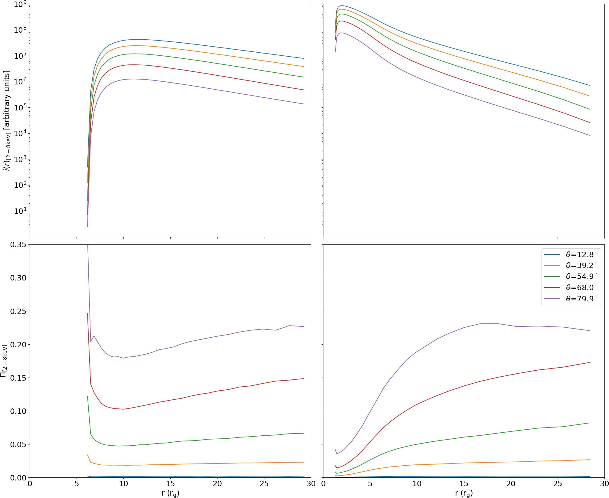
Figure 6: Photon flux (top row) and polarization degree (bottom row) plotted as functions of the radial distance $r$ in the two cases of $a=0$ (left-hand column) and $a=0.998$ (right-hand column), for the same values of parameters as in Figure 3 and for five different inclinations of the viewing direction. Stokes parameters have been energy integrated between $2$ and $8$ keV.

Figure 3 shows the spectra and polarization degree obtained in the two cases of $a=0$ and $a=0.998$, for five different viewing angles $\theta$. In order to correctly account for the different number of photons emitted from each radial bin, in these plots the Stokes parameter fluxes are summed over the radial distance $r$ in the following way,

$$\bar{i}(E,\theta) =\sum_{r}i(E,r,\theta)A(r)T^{4}(r)$$

$$\bar{q}(E,\theta) =\sum_{r}q(E,r,\theta)A(r)T^{4}(r)$$

$$\bar{u}(E,\theta) =\sum_{r}u(E,r,\theta)A(r)T^{4}(r)\,,$$ (16)

where $A(r)=2\pi r\mathrm{d}r$ is the area of the annular radial patch, with width $\mathrm{d}r$, at the distance $r$ from the center, while the factor $T^{4}(r)$ takes into account the different surface temperatures which characterize each radial patch.

¿From the top row of Figure 3 one can clearly see that the emerging photon flux is in general higher for a maximally rotating BH than for the case of $a=0$. This can be easily explained by the fact that, for $a=0.998$, the disc extends up to regions much closer to the BH horizon; here temperatures are much higher than for the non-rotating case, peaking at $\sim 1.7$ keV against a maximum value $\sim 0.6$ keV for $a=0$ (see Figure 2). As a consequence, for the Schwarzschild BH the seed photon blackbody peak can be expected to occur at $\sim 1$ keV, while starting from $3$–$4$ keV the strong energy dependence of the photoelectric absorption cross-section becomes more evident. On the other hand, the maximum of the injected blackbody falls at around $3$ keV in the maximally-rotating case, so that the contribution of seed photons is much more relevant all over the selected $1$–$10$ keV energy range. Absorption turns out to be important as well, as shown by the occurrence of several spectral features superimposed to the continuum in both the $a=0$ and $a=0.998$ cases. These lines appear to be mostly located at low energies ($1$–$2$ keV), with the exception of two, quite strong absorption features which appear at $\sim 6.5$ keV and $\sim 8$ keV.

The correspondent polarization degrees are plotted as functions of the photon energy in the bottom row of Figure 3. Looking at the figures, it is immediately clear that, as a general rule, polarization degree is higher when the absorption is more relevant (see also the comparison with the pure scattering case). This pattern can be explained by noting that, when absorption is important, most of the emerging photons are those originally emitted almost vertically and which suffer only one scattering: those photons are all polarized with the polarization vector parallel to the disc surface. Photons originally emitted at high inclinations are instead more likely to be absorbed; those photons, in the pure scattering limit, would provide mostly perpendicular polarization, with a reduction of the net polarization degree. Polarization of radiation emerging from the disc surface layer decreases by decreasing the observer’s inclination angle, attaining a value close to $0$ at small $\theta$ ($\la 13^{\circ}$) and at essentially all the photon energies. For $a=0$ (bottom-left panel), the polarization degree is in general higher than for the maximally-rotating BH case, except for the lower energies (at around $1$ keV), where $\Pi$ turns out to be very low (below $2\%$) at all the inclinations. This can be explained noting that, as mentioned above, primary photons peak indeed at such low energies, so that photons emerging at $1$–$2$ keV are essentially all seed photons, which are assumed to be unpolarized (see §3). At higher energies the polarization fraction increases rapidly, up to a maximum value close to $\sim 30\%$ for the highest inclinations. This behavior corresponds to the most important decline of the photon flux at around $2$ keV. For $a=0.998$ (bottom-right panel), the energy dependent behavior of the polarization degree closely follows that just discussed for the Schwarzschild case, notwithstanding the lower values attained, which are in general reduced by a factor of $\sim 2$–$3$ (with a maximum around $15\%$ at higher energies). As for the spectra, also the polarization fraction plots show further peculiar features between $6$ and $8$ keV, with the occurrence of quite narrow drops which seems to be associated, at first glance, to the analogous absorption lines in the flux. However, contrary of one could expect, the decrease in the photon flux would seem to correspond this time to a decrease also in the polarization degree.

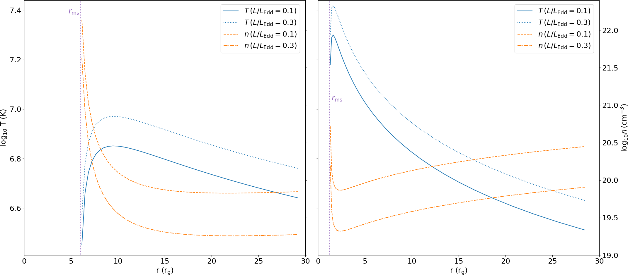
Figure 7: A comparison of the temperature (blue) and density (orange) radial profiles in the two cases of $a=0$ (left) and $0.998$ (right), for $L=0.1\,L_{\rm Edd}$ (the case also reported in Figure 2) and $0.3\,L_{\rm Edd}$.

This counter-intuitive behavior can be explained by noting that both the spectral and the polarization profiles reported here are strongly affected by our choice to adopt a 100-point energy grid between $1$ and $10$ keV. In order to better understand the nature of these features we report, for the sake of example, the results of an additional run of stokes in the case of $a=0.998$ and for the first radial bin of the disc surface, sampling the energy range with a 5000-point mesh. Figure 4 (left column) shows the plots of the spectrum and polarization degree for five different inclination angles and focussing on the energy band between $6$ and $8.5$ keV. Moreover, with the purpose of a greater clarity, we report in the right column the same situation as in the left one, in which we artificially removed all the features which are produced by resonant scattering. This allows one to clearly distinguish the contribution from the iron line complex, which in the selected energy range is essentially due to the transitions of Fe⁺²⁴ and Fe⁺²⁵ in various ionization states Sarazin (1988); Fabian et al. (2000), with two emission lines at $6.7$ and $7$ keV which stand out with respect to the continuum. Looking at the related polarization fraction plot (bottom-right panel), a sudden decrease of $\Pi$ occurs in correspondence with the aforementioned spectral features, as expected in the case of emission lines. Once resonant scattering is added in the computations (left panels), several absorption features appear in the spectrum, which are much broader than the narrow emission lines just discussed. In particular, two important absorption lines occur at exactly the same energies of the most important iron emission lines. A polarization degree growth correctly correponds to the scattering absorption lines, with the two significant drops at $6.7$ and $7$ keV due to the iron emission lines which are still visible in the middle of the polarization fraction peaks. We note that the features discussed here above can be fully resolved only if the energy grid is sufficiently fine (i.e. with more than $\sim 5000$ points between $1$ and $10$ keV). However, we remark that the energy resolution we adopted throughout the paper (i.e. 100 points in the $1$–$10$ keV range) is still far better than that of many existing instruments, and in particular of the forthcoming photoelectric polarimeters like IXPE. Furthermore, considering a too precise energy grid would lead to unacceptably long computational times, as well as to over-detailed spectral and polarization behaviors in the majority of the selected energy range, which are mostly pointless for our research. For these reasons we resort to the coarser, but still acceptable, 100-point energy resolution in the following.

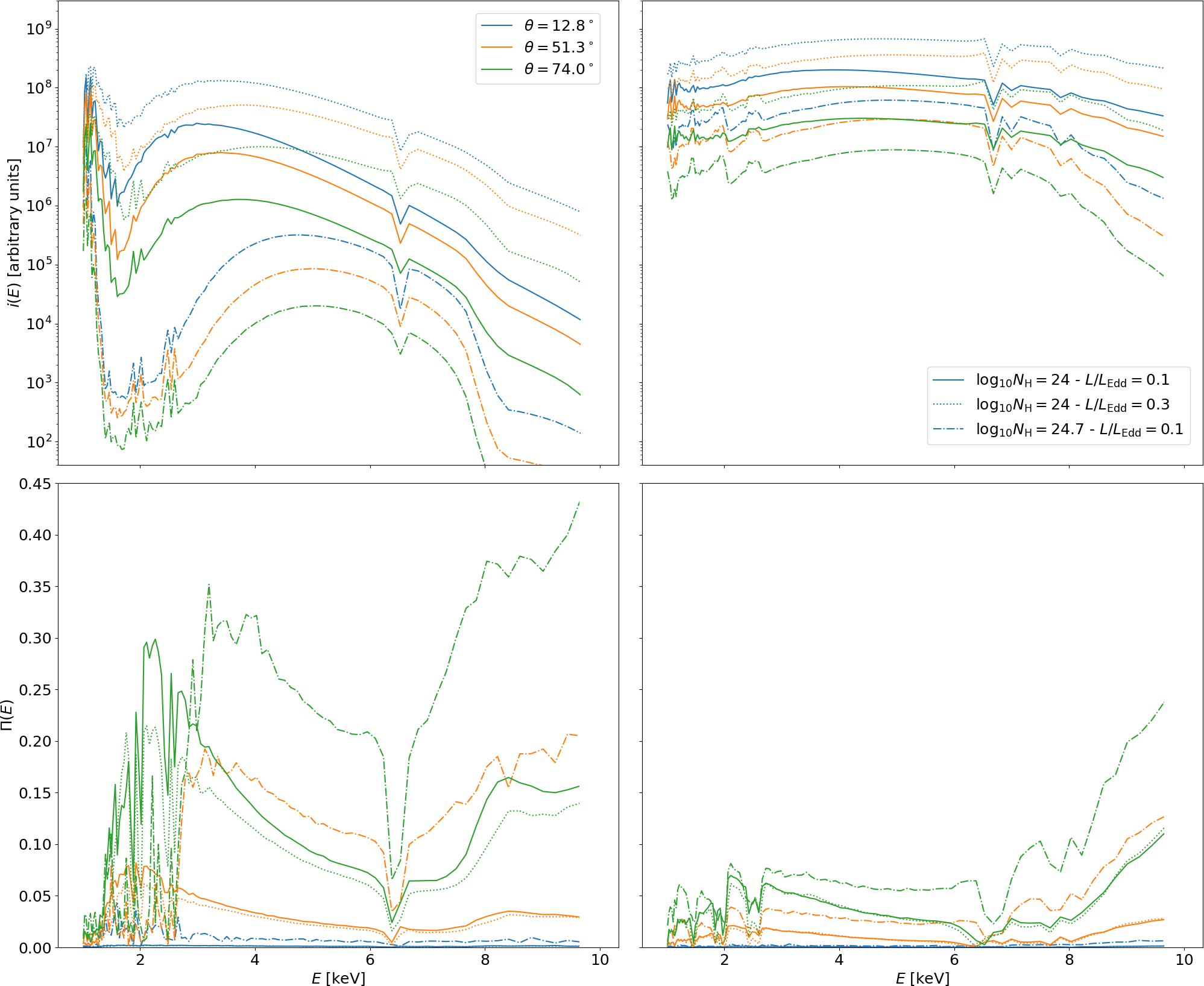
Figure 8: Spectrum (top row) and polarization degree (bottom row) of the radiation emitted from the disc surface in the cases of $a=0$ (left) and $0.998$ (right), for $N_{\rm H}^{\rm stop}=10^{24}\,{\rm cm}^{-2}$ – $L=0.1\,L_{\rm Edd}$ (solid lines), $N_{\rm H}^{\rm stop}=10^{24}\,{\rm cm}^{-2}$ – $L=0.3\,L_{\rm Edd}$ (dotted lines) and $N_{\rm H}^{\rm stop}=5\times 10^{24}\,{\rm cm}^{-2}$ – $L=0.1\,L_{\rm Edd}$ (dash-dotted lines), and for three different inclinations of the viewing direction: $\theta=12.8^{\circ}$ (blue), $51.3^{\circ}$ (orange) and $74.0^{\circ}$ (green). The values of the other parameters are chosen as in Figure 3.

In order to better understand how the ionization structure of the disc surface layer determines the polarization pattern of the emerging radiation, Figure 5 shows the behaviors of the polarization degree plotted as a function of the cosine of the inclination angle $\theta$. Here the Stokes parameters, which are still summed over the radial distance as described above (see equations 4.2), are further integrated over the photon energy in the $2$–$8$ keV IXPE energy band. The angular distribution of the polarization degree as predicted by Chandrasekhar’s (1960) formulae is also reported in the plots (red-dashed lines). The fact that $\Pi$ assumes only positive values at all the inclinations considered (for both the cases of $a=0$ and $a=0.998$) shows that emerging radiation is mostly polarized perpendicularly to the disc symmetry axis. This, as already discussed in §4.1, follows from the original assumption of radiation emitted isotropically from the base of the disc surface layer, so that photons are essentially emitted upwards, with propagation direction close to the disc axis. Furthermore, in the case of a maximally-rotating BH the polarization degree turns out to closely follow the Chandrasekhar’s profile, contrary of what happens for $a=0$, where the polarization fraction largely exceeds, at low inclinations, that predicted by Chandrasekhar (1960). Since the Chandrasekhar’s profile is the reference one for models that assume scattering as the only process responsible for photon polarization, one can safely conclude that the polarization properties in the $a=0.998$ case are mainly determined by scattering. On the other hand, absorption plays a more important role in the non-rotating case. This can be further confirmed looking again at the temperature and density distributions reported in Figure 2. In fact, due to the higher temperature reached close to the BH horizon, the fraction of ionized atoms is clearly expected to be larger for $a=0.998$, while for $a=0$ absorption effects become more important. In this regard, one should also notice that the total density close to the ISCO is much larger (by a factor of $\sim 30$) for the non-rotating case than for the maximally rotating one; this enhances the effects of absorption for $a=0$.

To complete this analysis, Figure 6 shows the photon flux and the polarization degree plotted as functions of the radial distance $r$ from the center, again for $a=0$ and $a=0.998$; also in this case Stokes parameters have been integrated over energy in the $2$–$8$ keV band. The behavior of the photon flux (top row) turns out to naturally follow the radial profile of the disc surface temperature reported in Figure 2, peaking at the distance $r$ characterized by the maximum temperature. On the other hand, as it can be seen in the bottom row, the polarization fraction tends to increase as the photon flux declines, apart from photons leaving the disc surface at small inclination angles, which (as already discussed) are practically unpolarized. Moreover, still taking as reference the plots in Figure 2, some similarities can be observed between the behaviors of the polarization degree and the total density as functions of the radial distance. This further confirm the previous findings that ascribe the rise in polarization fraction to absorption effects. In fact, in the Schwarzschild BH case $\Pi$ increases dramatically going towards the ISCO, where temperature is lower, since atoms are less ionized in this region and the density is quite large. Then, after a minimum attained in correspondence to the maximum of the temperature distribution (at $\sim 10\,r_{\rm g}$), the polarization degree rises again, although the density is more or less constant, as the temperature decreases (and the fraction of ionized atoms drops). In the maximally-rotating BH case, instead, the polarization fraction radial profile is mostly monotonic, going from the minimum value (attained close the ISCO) and essentially continuing to grow up to the outer boundary. This is due to both the temperature decrease and the density increase, which are visible in the right panel of Figure 2. The only exceptions occur very close to the ISCO, before the photon flux peak is reached, and farther than $\sim 20\,r_{\rm g}$, with a slight decrease of the polarization fraction for the highest inclinations ($\ga 80^{\circ}$). While the former effect is analogous to that just discussed for small radii in the $a=0$ case, the latter can be more likely ascribed to the absorption features which are present at low energies in the behavior of $\Pi$. In fact, according to the adopted radial profile, the surface temperature far from the central BH turns out to be quite low ($\sim 0.3$ keV), so that only low-energy photons are expected to contribute significantly at those distances. Recalling that the plots in Figure 6 have been obtained summing the Stokes parameters in the $2$–$8$ keV energy range, it is reasonable to conclude that the slight decline of $\Pi$ at large $r$ and high inclinations is due to the deep features which characterize the polarization degree at around $2$–$3$ keV (see the bottom-right panel of Figure 3), which are indeed more relevant for high values of $\theta$.

4.3 Exploring different luminosities and optical depths

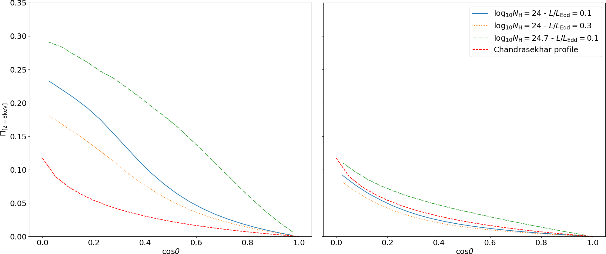
Figure 9: Polarization degree plotted as a function of the cosine of the inclination angle $\theta$ in the two cases $a=0$ (left-hand column) and $a=0.998$ (right-hand column), for $N_{\rm H}^{\rm stop}=10^{24}\,{\rm cm}^{-2}$ – $L=0.1\,L_{\rm Edd}$ (blue, solid), $N_{\rm H}^{\rm stop}=10^{24}\,{\rm cm}^{-2}$ – $L=0.3\,L_{\rm Edd}$ (orange, dotted) and $N_{\rm H}^{\rm stop}=5\times 10^{24}\,{\rm cm}^{-2}$ – $L=0.1\,L_{\rm Edd}$ (green, dash-dotted), while the other parameters have the same values as in Figure 3. Stokes parameters have been summed over the radial distance from the central BH (see equations 4.2) and energy integrated between $2$ and $8$ keV. The red-dashed lines denotes the behavior calculated according the formulae by Chandrasekhar (1960, see Table XXIV).

After having discussed the behavior of spectral and polarization observables for a given set of parameter values, we now test how the Stokes parameters of the emerging radiation can change by varying the properties of the disc material and the accretion flow. In this respect, we explored two further configurations, characterized by different values of mass accretion rate $\dot{M}$ and stop column density $N_{\rm H}^{\rm stop}$, leaving the BH mass unchanged at $10\,{\rm M}_{\odot}$ and the hardening factor $f_{\rm col}=1.8$. As reported in equations (2) and (• ‣ A)–(• ‣ A), varying the accretion luminosity acts both on the temperature and the density radial profiles. Figure 7 shows the variations of temperature and density profiles as a result of increasing the accretion rate from $10\%$ (i.e. the case already described in §4.2) to $30\%$ of the Eddington limit, again for the two cases of non-rotating and maximally rotating BHs. In particular, the temperature undergoes a general shift upwards by a factor of $\sim 1.3$, superimposed to a radial displacement of the maximum towards a slightly larger distance from the center. The density, on the other hand, drops at all the considered radial distances by a factor of $\sim 3$.

The effects of such changes on the emerging flux are shown in the top row of Figure 8, where solid lines mark the behavior for $L=0.1\,L_{\rm Edd}$ (i.e. the case already discussed in §4.2) and dotted lines that for $L=0.3\,L_{\rm Edd}$ ($N_{\rm H}^{\rm stop}=10^{24}\,{\rm cm}^{-2}$ for both these runs). As one could expect, the photon flux attains higher values when a higher accretion luminosity is considered, due to the increase of the temperature all over the disc surface. For $a=0$ (top-left panel), the low-energy peak due to primary photons is sensibly broadened with respect to the $L=0.1\,L_{\rm Edd}$ case. Moreover, the spectral features ascribed to absorption are less pronounced, as a result of both the temperature increase (which also increases the ionization fraction in the disc material) and the lower values of density. Also in the $a=0.998$ case (top-right panel), spectra for $L=0.3\,L_{\rm Edd}$ turn out to be harder than for lower luminosities. In this case no substantial differences can be observed in the absorption features, since, as noted before, already at $L=0.1\,L_{\rm Edd}$ temperature was sufficiently high to significantly reduce absorption effects. Dash-dotted lines in Figure 8 mark, instead, the behavior of the emerging flux for $N_{\rm H}^{\rm stop}=5\times 10^{24}\,{\rm cm}^{-2}$, which corresponds to a Thomson optical depth $\tau\simeq 3.33$. In order to display only the effect of changing $N_{\rm H}^{\rm stop}$, for this simulation we returned to $L=0.1\,L_{\rm Edd}$, so that temperature and density profiles are those reported in Figure 2. Contrary of what happens by increasing the accretion luminosity, in this case the number of emerging photons turns out to be pretty lower in the entire energy range. The peaks of the spectral distributions fall at the same energy as in the original case (see §4.2), as a result of the choice to adopt the same temperature profile. However, both in the Schwarzschild and in the maximally-rotating case absorption features are dramatically more significant, this effect being more evident for $a=0$. Indeed, assuming that photons escape the layer at a $z_{\rm max}$ corresponding to a larger optical depth implies that they are still involved in a conspicuous number of scatterings, so that a lower number of emerging photons at that altitude $z_{\rm max}$ can be reasonably expected. Moreover, since an increase of the optical depth translates into a decrease of the photon mean free path inside the disc material, this also justifies the increase of absorption effects, despite the fact that temperature and density are unchanged with respect to the initial case (with $N_{\rm H}^{\rm stop}=10^{24}\,{\rm cm}^{-2}$).

Much in the same way as the spectra, the polarization degree of the emerging radiation is influenced as well by the changes in luminosity and optical depth. The bottom row of Figure 8 shows the energy-dependence of $\Pi$, plotted for the same values of the parameters adopted for the flux in the top row. By increasing $L$ to $0.3\,L_{\rm Edd}$, the overall behavior turns out to be in general lowered by $\sim 1$–$2\%$ with respect to the initial case, with a more important reduction at lower energies and for high values of $\theta$. On the other hand, substantial differences can be observed when the value of $N_{\rm H}^{\rm stop}$ is increased. In particular, a steep rise occurs as the inclination angle increases, attaining a value $\sim 40\%$ for $a=0$ and $\sim 20\%$ for $a=0.998$ at $10$ keV. To explore this behavior more in depth, we reported in Figure 9 the plots of the energy-integrated polarization fraction as a function of the viewing inclination, similarly to those shown in Figure 5; also in this case the polarization degree predicted by Chandrasekhar’s (1960) prescription is displayed for comparison. By increasing the accretion rate (dotted lines), $\Pi$ turns out to be substantially reduced at high inclinations for $a=0$ (down to $\sim 75\%$ of the value attained for $L=0.1\,L_{\rm Edd}$), but still remaining above the level set by the Chandrasekhar’s profile. For $a=0.998$, instead, $\Pi$ is only slightly lower than in the initial case, similarly to what we have noted in Figure 8, with an overall reduction not larger than $\sim 1\%$. On the contrary, if the stop column density is increased to $5\times 10^{24}\,{\rm cm}^{-2}$ (maintaining the luminosity at $0.1\,L_{\rm Edd}$) then the polarization degree in general increases too (dash-dotted lines). Also in this case the most relevant change occurs in the Schwarzschild limit (attaining a maximum value close to $30\%$ at high inclinations), while the curve is not far from the original one (and from that given by the Chandrasekhar’s profile) in the maximally-rotating limit. All these behaviors comply with those just discussed for the flux. In fact, the temperature increase (with the consequent ionization fraction rise) and the density decrease which occur taking $L=0.3\,L_{\rm Edd}$ both determine a lower influence of absorption effects, so that the polarization fraction turns out to be lower with respect to the case with a lower luminosity. On the other hand, considering a larger value of the stop column density means that photon transfer is calculated for larger optical depths. This translates into more significant absorption effects which produce an increase of the polarization degree. That being said, what we have concluded in the reference case (see §4.2) holds true also for different luminosities and column densities, i.e. radiation is basically more polarized for $a=0$ than for $a=0.998$, confirming that absorption is more important for slowly rotating BHs, while scattering dominates as the BH spin increases.

5 Discussion and conclusions

In this paper we discussed a method to simulate the spectral and polarization properties of radiation emitted from stellar-mass BH accretion discs in the soft state. Contrary to previous works, where, following the Chandrasekhar’s (1960) prescription, polarization was considered to be due only to scattering of photons onto electrons in the disc, in our model we include a self-consistent treatment of absorption effects in the disc material. To this aim, we solved the ionization structure in the surface layer of the disc using the photo-ionization code cloudy Ferland et al. (2017), assuming the Novikov & Thorne (1973) temperature profile and the Compère & Oliveri (2017) density profile. Seed radiation (assumed to be unpolarized) is injected isotropically from the bottom of this layer, according to a blackbody distribution at the local temperature. The radiative transfer of photons is then calculated using the ray-tracing, Monte Carlo code stokes Marin (2018); Goosmann & Gaskell (2007). The emerging photon Stokes parameters are determined for a number of virtual detectors on the surface of the layer, displaced at different inclinations with respect to the disc axis.

The main findings of our present investigation can be summarized in the following points.

• Placing the emitting source at the base of the surface layer forces the polarization direction of most of the emerging photons to be parallel to the plane of the disc (see Figure 1). This differs from the results of previous works (e.g. Dovčiak et al., 2008, with emission region placed in the middle of the slab), according to which a consistent fraction of photons is polarized parallel to the disc symmetry axis for $\tau\la 2$. In fact, when only scattering is considered, the polarization degree at lower $\tau$ is quite small for emitting source on the bottom with respect to the case of emission from the middle of the layer. As expected, the polarization fraction tends to the angular behavior described by Chandrasekhar’s (1960) formulae at high optical depths ($\tau\ga 5$).

• We emphasize that including absorption effects goes in general towards increasing the polarization degree (see Figure 3 and 5, left columns). This is particularly encouraging, considering that all the theoretical models developed so far (which account for scattering as the only responsible for photon polarization, see e.g. Dovčiak et al., 2008; Schnittman & Krolik, 2009; Taverna et al., 2020) predict a level of polarization of $\sim 10\%$ at most.

• The photon spectrum and the polarization degree turn out to strongly depend on the spin of the central BH. This can be essentially ascribed to the fact that, as the BH spin increases, the inner boundary of the disc extends to smaller distances from the horizon, where temperatures are higher and more energetic photons can be emitted (see Figures 2 and 6). In addition, according to the profile by Compère & Oliveri (2017), the density turns out to be higher for lower values of $a$ (see again Figure 2). As a consequence, photon polarization can be reasonably expected to be higher for slowly rotating BHs, for which absorption effects are more important, while polarization tends to approach the Chandrasekhar’s profile for $a=0.998$ (Figure 5, right panel), where scattering effects are dominant.

• Including self-consistently the absorption effects in our model allows us to specify the non-trivial behavior of the seed photon Stokes parameters as a function of photon energy, observer’s inclination and radial distance from the center, as it can be seen in Figure 3, 4 and 6.

• We could test the dependence of spectra and polarization on the physical properties of the disc, such as the accretion luminosity and the hydrogen column density of the disc surface slab (see Figures 8 and 9). In particular, we have checked that increasing the accretion luminosity acts in increasing the photon flux and decreasing the polarization degree, as a result of the correspondent temperature rise and density drop (see Figure 7). On the other hand, placing the upper boundary of the layer at a different height modifies as well the polarization properties, increasing $\Pi$ as a higher value of $N_{\rm H}^{\rm stop}$ is considered.

We stress again that the main goal of this paper is to explore the effects of absorption on the polarization properties of the thermal disc emission, so we give spectra and polarization observables of radiation without considering the effects of strong gravity on photon energy and trajectory; general relativistic corrections, including returning radiation, will be properly addressed in a future work. We also stress that our physical assumption of an ionized slab above a standard, black body emitting disc is certainly simplistic. A global, completely self-consistent treatment of the disc structure including polarized radiative transfer is a very ambitious goal, and clearly beyond the scope of this work. Nevertheless, the results of the present investigation show that including absorption effects alongside those of scattering is crucial for correctly modeling the polarization properties of emission from stellar-mass BH accretion discs, an important result in view of the forthcoming X-ray polarimetry missions that will be launched in the next decade.

Data availability

The data underlying this article will be shared on reasonable request to the corresponding author.

Appendix A Density radial profile in the disc

The equatorial density of the disc material can be expressed as follows, in each of the three different regions in which the disc is divided, according to which component between gas and radiation dominates in the pressure and which process between scattering and free-free dominates the opacity Compère & Oliveri (2017); Taverna et al. (2020):

• in the inner region, where radiation pressure and scattering opacity dominate over gas pressure and free-free opacity, respectively,

  $$n_{0}({\rm H})_{\rm inn}=(1.50\times 10^{19}\,{\rm cm}^{-3})\,\alpha^{-1}\left(\frac{M}{3{\rm M}_{\odot}}\right)$$

  $$\,\,\,\,\,\,\times\left(\frac{\dot{M}}{10^{17}\,{\rm g\,s}^{-1}}\right)^{-2}\xi^{5}\mathcal{C}^{3}\mathcal{D}^{-1}\mathcal{R}^{2}\mathcal{P}^{-2}\,;$$ (17)

• in the middle region, where scattering is still the main source of opacity but gas pressure dominates over radiation pressure,

  $$n_{0}({\rm H})_{\rm mid}=(4.86\times 10^{24}\,{\rm cm}^{-3})\,\alpha^{-7/10}\left(\frac{M}{3{\rm M}_{\odot}}\right)^{-11/10}$$

  $$\,\,\,\,\,\,\times\left(\frac{\dot{M}}{10^{17}\,{\rm g\,s}^{-1}}\right)^{2/5}\xi^{-37/10}\mathcal{C}^{3/10}\mathcal{D}^{-7/10}\mathcal{R}^{1/2}\mathcal{P}^{2/5}\,;$$ (18)

• in the outer region, where gas pressure and free-free opacity dominate over radiation pressure and scattering opacity, respectively,

  $$n_{0}({\rm H})_{\rm out}=(3.06\times 10^{25}\,{\rm cm}^{-3})\,\alpha^{-7/10}\left(\frac{M}{3{\rm M}_{\odot}}\right)^{-5/4}$$

  $$\,\,\,\,\,\,\times\left(\frac{\dot{M}}{10^{17}\,{\rm g\,s}^{-1}}\right)^{11/20}\xi^{-43/10}\mathcal{C}^{3/20}\mathcal{D}^{-7/10}\mathcal{R}^{17/40}\mathcal{P}^{11/20}\,.$$ (19)

In equations (• ‣ A)–(• ‣ A) we assumed the mean rest mass per barion $m_{\rm b}$ as $1/56$ the mass of an ${}^{56}{\rm Fe}$ atomic nucleus Thorne & Blandford (2017) and $\alpha$ is the disc parameter (see Shakura & Sunayev, 1973, we take $\alpha=0.2$ throughout the paper), while complete expressions for the functions $\mathcal{C}$, $\mathcal{D}$, $\mathcal{R}$ and $\mathcal{P}$ are reported in Compère & Oliveri (2017).

References

- Asplund et al. (2005) Asplund, M., Grevesse, N., Sauval, A. J., Cosmic Abundances as Records of Stellar Evolution and Nucleosynthesis in honor of David L. Lambert, ASP Conference Series, Vol. 336, Proceedings of a symposium held 17-19 June, 2004 in Austin, Texas. Edited by Thomas G. Barnes III and Frank N. Bash. San Francisco: Astronomical Society of the Pacific, 2005, p. 25
- Agol & Krolik (2000) Agol E., Krolik J. K., 2000, ApJ, 528, 161
- Bardeen et al. (1972) Bardeen J. M., Press W. H., Teukolsky S. A., 1972, ApJ, 178, 347
- Chandrasekhar (1960) Chandrasekhar S., 1960, Radiative transfer, Dover, New York
- Compère & Oliveri (2017) Compère G., Oliveri R., 2017, MNRAS, 468, 4351
- Connors & Stark (1977) Connors P. A., Stark R. F., 1977, Nature, 269, 128
- Connors, Piran & Stark (1980) Connors P. A., Piran T., Stark R. F., 1980, ApJ, 235, 224
- Davis & El-Abd (2019) Davis S. W., El-Abd S., 2019, ApJ, 874,23
- Dovčiak et al. (2008) Dovčiak M., Muleri F., Goosmann R. W., Karas V., Matt G., 2008, MNRAS, 391, 32
- Dovčiak et al. (2011) Dovčiak M., Muleri F., Goosmann R. W., Karas V., Matt G., 2011, ApJ, 731, 75
- Fabian et al. (2000) Fabian A. C., Iwasawa K., Reynolds C. S., Young A. J., 2000, PASP, 112, 1145
- Ferland et al. (2017) Ferland G. J. et al., 2017, The 2017 Release Cloudy. Revista Mexicana de Astronomia y Astrofisica, 53, 385
- Gnedin & Silant’ev (1978) Gnedin Yu. N., Silant’ev N. A., 1978, Soviet Astronomy, 22, 325
- Goosmann & Gaskell (2007) Goosmann R. W., Gaskell C. M., 2007, A&A, 465, 129
- Johannsen & Psaltis (2011) Johannsen T., Psaltis D., 2011, Phys. Rev. D 83, 124015
- Karas (2006) Karas V., 2006, AN, 327, 961
- Krawczynski (2012) Krawczynski H., 2012, ApJ, 754, 133
- Laor, Netzer & Piran (1990) Laor A., Netzer H., Piran T., 1990, MNRAS, 242, 560
- Li, Narayan & McClintock (2009) Li L.-X-, Narayan R., McClintock J. E., 2009, ApJ, 691, 847
- Marin et al. (2012) Marin F., Goosmann R. W., Gaskell C. M., Porquet D., Dovčiak M., 2012, A&A, 548, 121
- Marin (2018) Marin F., 2018, A&A, 615, 171
- Matt, Fabian & Ross (1993a) Matt G., Fabian A. C., Ross R. R., 1993, MNRAS, 262, 179
- Matt, Fabian & Ross (1993b) Matt G., Fabian A. C., Ross R. R., 1993, MNRAS, 264, 839
- Motta et al. (2014) Motta S., Belloni T.M., Stella L., Munoz-Darias T., Fender R., 2014, MNRAS, 437, 2554
- Nagirner (1962) Nagirner D. I., 1962, Tr. Astron. Obs. Leningr. Gos. Univ., 30, 79
- Novikov & Thorne (1973) Novikov I. D. , Thorne K. S. , 1973, in Black Holes (Les Astres Occlus), C. Dewitt, and B. S. Dewitt, 343
- Page & Thorne (1974) Page D. N., Thorne K. S., 1974, ApJ, 191, 499
- Reynolds (2019) Reynolds, C.R., 2019, Nature Astronomy, 3, 41
- Sarazin (1988) Sarazin C. L., 1988, X-Ray Emissions from Clusters of Galaxies, Cambridge Astrophysics Series, Cambridge: Cambridge University Press