Microscopic origin of reflection-asymmetric nuclear shapes

Abstract

Background

The presence of nuclear ground states with stable reflection-asymmetric shapes is supported by rich experimental evidence. Theoretical surveys of odd-multipolarity deformations predict the existence of pear-shaped isotopes in several fairly localized regions of the nuclear landscape in the vicinity of near-lying single-particle shells with $\Delta\ell=\Delta j=3$.

Purpose

We analyze the role of isoscalar, isovector, neutron-proton, neutron-neutron, and proton-proton multipole interaction energies in inducing the onset of reflection-asymmetric ground-state deformations.

Methods

The calculations are performed in the framework of axial reflection-asymmetric Hartree-Fock-Bogoliubov theory using two Skyrme energy density functionals and density-dependent pairing force.

Results

We show that reflection-asymmetric ground-state shapes of atomic nuclei are driven by the odd-multipolarity neutron-proton (or isoscalar) part of the nuclear interaction energy. This result is consistent with the particle-vibration picture, in which the main driver of octupole instability is the isoscalar octupole-octupole interaction giving rise to large $E3$ polarizability.

Conclusions

The necessary condition for the appearance of localized regions of pear-shaped nuclei in the nuclear landscape is the presence of parity doublets involving $\Delta\ell=\Delta j=3$ proton or neutron single-particle shells. This condition alone is, however, not sufficient to determine whether pear shapes actually appear, and – if so – what the corresponding reflection-asymmetric deformation energies are. The predicted small reflection-asymmetric deformation energies result from dramatic cancellations between even- and odd-multipolarity components of the nuclear binding energy.

I Introduction

While the vast majority of atomic nuclei have either spherical or ellipsoidal (prolate or oblate) ground-state (g.s.) shapes, some isotopes exhibit pear-like shape deformations that intrinsically break reflection symmetry. Experimental evidence for such shapes comes from characteristic properties of nuclear spectra, nuclear moments, and electromagnetic matrix elements Butler and Nazarewicz (1996); Butler (2020). Pear-shaped even-even nuclei display low-energy negative-parity excitations that are usually attributed to octupole collective modes. For that reason, pear-shaped nuclei are often referred to as “octupole-deformed.”

There are two regions of g.s. reflection-asymmetric shapes that have been experimentally established over the years: the neutron-deficient actinides around ²²⁴Ra and the neutron-rich lanthanides around ¹⁴⁶Ba. Nuclear theory systematically predicts these nuclei to be pear-shaped (see Ref. Cao et al. (2020) for a recent survey of theoretical results). Other regions of pear-shaped nuclei predicted by theory, i.e., lanthanide nuclei around ²⁰⁰Gd as well as actinide and superheavy nuclei with $184<N<206$ are too neutron rich to be accessible by experiment Erler et al. (2012); Agbemava et al. (2016); Agbemava and Afanasjev (2017); Xu and Li (2017); Cao et al. (2020). In general, deformation energies associated with reflection-symmetry breaking shapes are much smaller than those related to stable ellipsoidal shapes Myers and Swiatecki (1966); Möller et al. (2008). Consequently, for octupole-deformed nuclei, beyond mean-field methods are needed for a quantitative description, see, e.g., Refs. Egido and Robledo (1991); Robledo (2016); Xia et al. (2017); Fu et al. (2018).

According to the single-particle (s.p.) picture, the appearance of pear-shaped deformations can be attributed to the mixing of opposite-parity s.p. shells Strutinsky (1956); Lee and Inglis (1957). In the macroscopic-microscopic (MM) approach, the macroscopic energy favors spherical shapes. Therefore, stable refection-asymmetric shape deformations obtained in the MM method Nazarewicz et al. (1984); Möller et al. (2008) can be traced back to the shape polarization originating from proton and neutron s.p. levels interacting via parity-breaking fields. Since shell corrections are computed separately for protons and neutrons, the results are usually interpreted in terms of deformation-driving proton or neutron shell effects. The proton-neutron interactions are indirectly considered in the macroscopic energy with the assumption of identical proton and neutron shape deformation parameters, which follow those of the macroscopic term.

In general, in the description based on the mean-field approach, nuclear shape deformations result from a coupling between collective surface vibrations of the nucleus and valence nucleons. Such a particle-vibration coupling Bohr (1952) mechanism can be understood in terms of the nuclear Jahn-Teller effect Reinhard and Otten (1984); Nazarewicz (1994). The tendency towards deformation is particularly strong if the Fermi level lies just between close-lying s.p. states. In such a case, the system can become unstable with respect to the mode that couples these states. Simple estimates of the particle-vibration coupling (Jahn-Teller vibronic coupling) for the quadrupole mode (multipolarity $\lambda=2$) Bohr and Mottelson (1975); Bes et al. (1975) demonstrate that its contribution to the mass quadrupole moment at low energies doubles the quadrupole moment of valence nucleons. The Hartree-Fock (HF) analysis Dobaczewski et al. (1988); Werner et al. (1994) confirmed this estimate. It showed that the main contribution to the quadrupole deformation energy comes from the attractive isoscalar quadrupole-quadrupole term, which can be well approximated by the neutron-proton quadrupole interaction.

When it comes to reflection-asymmetric deformations, the leading particle-vibration coupling is the one due to the octupole mode (multipolarity $\lambda=3$). This coupling generates a vibronic Jahn-Teller interaction between close-lying opposite-parity s.p. orbits that may result in a static reflection-asymmetric shape. For g.s. configurations of atomic nuclei, such pairs of states can be found just above closed shells and involve a unique-parity intruder shell $(\ell,j)$ and a normal-parity shell $(\ell-3,j-3)$ around particle numbers $N_{\rm oct}=34$, 56, 88, and, 134 Butler and Nazarewicz (1996). Indeed self-consistent calculations systematically predict pear shapes for nuclei having proton and neutron numbers close to $N_{\rm oct}$.

To understand the origin of reflection-asymmetric g.s. deformations, in this study we extend the quadrupole-energy analysis of Refs. Dobaczewski et al. (1988); Werner et al. (1994) to odd-multipolarity shapes. To this end we decompose the total Hartree-Fock-Bogoliubov (HFB) energy into isoscalar, isovector, neutron-neutron ($nn$), proton-proton ($pp$), and neutron-proton ($np$) contributions of different multipolarities.

This paper is organized as follows. In Sec. II we estimate the octupole polarizability and coupling strengths of the octupole-octupole interaction. Section III describes the multipole decomposition of one-body HFB densities and the HFB energy. The results of our analysis calculations and an analysis of trends are presented in Sec. IV. Finally, Sec. V contains the conclusions of this work.

II Simple estimate of low-energy octupole coupling

In this section, we follow Refs. Bohr and Mottelson (1975); Bes et al. (1975), which used a schematic particle-vibration coupling Hamiltonian consisting of a spherical harmonic-oscillator one-body term and a multipole-multipole residual interaction. This model was used in the early paper Dobaczewski et al. (1988) in the context of quadrupole deformations. The model Hamiltonian with the octupole-octupole interaction is

$$\hat{H}=\hat{H}_{0}+\frac{1}{2}\kappa_{0}\hat{Q}_{0}\hat{Q}_{0}+\frac{1}{2}\kappa_{1}\hat{Q}_{1}\hat{Q}_{1},$$ (1)

where $\hat{Q}_{0}=\hat{Q}_{n}+\hat{Q}_{p}$ and $\hat{Q}_{1}=\hat{Q}_{n}-\hat{Q}_{p}$ are single-particle octupole isoscalar and isovector operators, respectively, and $\hat{H}_{0}$ is a spherical one-body harmonic-oscillator Hamiltonian. For the case of high-frequency octupole oscillations (giant octupole resonances), the coupling constants of the isoscalar and isovector octupole-octupole interactions, $\kappa_{0}$ and $\kappa_{1}$, respectively, can be written as:

$$\kappa_{0}=-\frac{4\pi}{7}\frac{M\omega_{0}^{2}}{A\langle r^{4}\rangle},~{}~{}\kappa_{1}=\frac{\pi V_{\rm sym}}{A\langle r^{6}\rangle},$$ (2)

where $\omega_{0}$ is the oscillator frequency, $V_{\rm sym}$ is the repulsive symmetry potential ($\sim 130$ MeV), and $M$ is the nucleon mass. Since the isovector coupling constant $\kappa_{1}$ is positive, the g.s. neutron and proton deformations are expected to be similar, as assumed in the MM approaches.

Within the Hamiltonian (1), the g.s.  octupole polarizability of the nucleus is given by Bohr and Mottelson (1975)

$$\chi_{3,\tau}=-\frac{\kappa_{\tau}}{\kappa_{\tau}+C_{3}^{(0)}},$$ (3)

where $\tau=0$ or 1 and $C_{3}^{(0)}$ is the restoring force parameter. There are two types of octupole modes involving s.p. transitions with $\Delta{\cal N}=1$ or 3, where ${\cal N}$ is the principal oscillator quantum number. The corresponding restoring-force parameters are:

$$C_{3}^{(0)}(\Delta{\cal N}=1) =\frac{16\pi}{21}\frac{M\omega_{0}^{2}}{A\langle r^{4}\rangle},$$ (4)

$$C_{3}^{(0)}(\Delta{\cal N}=3) =3C_{3}^{(0)}(\Delta{\cal N}=1).$$ (5)

By using the estimate in Ref. Bohr and Mottelson (1975)

$$\frac{V_{\rm sym}}{M\omega_{0}^{2}}\approx 2.9\frac{\langle r^{4}\rangle}{\langle r^{2}\rangle},$$ (6)

one obtains:

$$\chi_{3,0}(\Delta{\cal N}=1)=3,~{}~{}~{}\chi_{3,0}(\Delta{\cal N}=3)=1/3.$$ (7)

The isovector octupole polarizabilities are obtained in a similar way by assuming a uniform density distribution:

$$\chi_{3,1}(\Delta{\cal N}=1)=-0.78,~{}~{}~{}\chi_{3,1}(\Delta{\cal N}=3)=-0.54.$$ (8)

While the collective octupole modes couple the $\Delta{\cal N}=1$ and 3 transitions, the low-frequency mode is primarily associated with the $\Delta{\cal N}=1$ excitations. At low energies, associated with nuclear ground states, the strength coefficients in Eq. (2) should be renormalized by factors $(1+\chi_{3,\tau})$ to account for the coupling to high-energy octupole collective vibrations. We indicate them by $\tilde{\kappa}_{\tau}=(1+\chi_{3,\tau})\kappa_{\tau}.$ Following Ref. Dobaczewski et al. (1988), we rearrange the octupole-octupole Hamiltonian into $nn$, $pp$, and $np$ parts with the coupling constants

$$\tilde{\kappa}_{nn}=\tilde{\kappa}_{pp}=\tilde{\kappa}_{0}+\tilde{\kappa}_{1},~{}~{}\tilde{\kappa}_{np}=\tilde{\kappa}_{0}-\tilde{\kappa}_{1}.$$ (9)

By assuming the average values of octupole polarizabilities $\chi_{3,0}\approx 2$ and $\chi_{3,1}\approx-0.4$, the ratio of the coupling constants becomes:

$$\frac{\tilde{\kappa}_{nn}}{\tilde{\kappa}_{np}}=\frac{\tilde{\kappa}_{pp}}{\tilde{\kappa}_{np}}\approx 0.27.$$ (10)

We can thus conclude that the octupole-octupole $np$ interaction may indeed be viewed as being responsible for the development of the octupole deformation.

III Multipole expansion of densities and HFB energy

In self-consistent mean-field approaches Ring and Schuck (1980); Bender et al. (2003); Schunck (2019) with energy-density functionals (EDFs) based on two-body functional generators, the total energy of a nucleus is expressed as:

$$E=\mathrm{Tr}(T\rho)+\tfrac{1}{2}\mathrm{Tr}(\Gamma\rho)+\tfrac{1}{2}\mathrm{Tr}(\tilde{\Gamma}\tilde{\rho}).$$ (11)

Here $T$ is the kinetic energy operator, $\Gamma$ and $\tilde{\Gamma}$ are mean fields in particle-hole (p-h) and particle-particle (p-p) channels, respectively, and $\rho$ and $\tilde{\rho}$ are one-body p-h and p-p density matrices, respectively. (Instead of using the standard pairing tensor Ring and Schuck (1980), here we use the “tilde” representation of the p-p density matrix Dobaczewski et al. (1984).) The mean fields $\Gamma$ and $\tilde{\Gamma}$ are defined as

$$T+\Gamma =\frac{\delta E}{\delta^{\prime}\rho},$$ (12)

$$\tilde{\Gamma} =\frac{\delta E}{\delta^{\prime}\tilde{\rho}},$$ (13)

where $\delta^{\prime}$ denotes the variation of the total energy that neglects the dependence of the functional generators on density, that is, the mean fields (12) and (13) do not contain so-called rearrangement terms Bender et al. (2003).

III.1 Multipole decomposition

As observed in Ref. Dobaczewski et al. (1988), the density matrices and mean fields can be split into different multipole components as

$$\rho =\rho_{[0]}+\rho_{[1]}+\rho_{[2]}+\rho_{[3]}+\ldots$$ (14a)

$$\tilde{\rho} =\tilde{\rho}_{[0]}+\tilde{\rho}_{[1]}+\tilde{\rho}_{[2]}+\tilde{\rho}_{[3]}+\ldots,$$ (14b)

$$\Gamma =\Gamma_{[0]}+\Gamma_{[1]}+\Gamma_{[2]}+\Gamma_{[3]}+\ldots$$ (14c)

$$\tilde{\Gamma} =\tilde{\Gamma}_{[0]}+\tilde{\Gamma}_{[1]}+\tilde{\Gamma}_{[2]}+\tilde{\Gamma}_{[3]}+\ldots,$$ (14d)

where $\rho_{[\lambda]}$, $\tilde{\rho}_{[\lambda]}$, $\Gamma_{[\lambda]}$, and $\tilde{\Gamma}_{[\lambda]}$ are rank-$\lambda$ rotational components of $\rho$, $\tilde{\rho}$, $\Gamma$, and $\tilde{\Gamma}$, respectively. Traces appearing in Eq. (11) are invariant with respect to unitary transformations, and, in particular, with respect to spatial rotations. Therefore, the traces act like multipolarity filters projecting the total energy on a rotational invariant. In this way, when the multipole expansions (14) are inserted in the expression for the total energy (11), only diagonal terms remain:

$$E=E_{[0]}+E_{[1]}+E_{[2]}+E_{[3]}+\ldots,$$ (15)

where

$$E_{[\lambda]}=\tfrac{1}{2}\mathrm{Tr}(\Gamma_{[\lambda]}\rho_{[\lambda]})+\tfrac{1}{2}\mathrm{Tr}(\tilde{\Gamma}_{[\lambda]}\tilde{\rho}_{[\lambda]}).$$ (16)

In the above equation, we add the kinetic energy to the monopole energy $E_{[0]}$ since $T$ is a scalar operator which implies $E_{\rm kin}=\mathrm{Tr}(T\rho)\equiv\mathrm{Tr}(T\rho_{[0]})$. Therefore we define

$$E_{[0]}=E_{\rm kin}+\tfrac{1}{2}\mathrm{Tr}(\Gamma_{[0]}\rho_{[0]})+\tfrac{1}{2}\mathrm{Tr}(\tilde{\Gamma}_{[0]}\tilde{\rho}_{[0]}).$$ (17)

When parity symmetry is conserved, only even-$\lambda$ multipolarities appear in Eqs. (14) and (15). In Refs. Dobaczewski et al. (1988); Werner et al. (1994), this allowed for analyzing the monopole ($\lambda=0$), quadrupole ($\lambda=2$), and higher even-$\lambda$ components. In the present work, we analyze broken-parity self-consistent states and focus on the reflection-asymmetric (odd-$\lambda$) components of the expansion. As our multipole expansion is defined with respect to the center of mass of the nucleus, the integral of the isoscalar dipole density $\rho_{[1]}$, namely, the total isoscalar dipole moment, vanishes by construction. Nevertheless, the dipole density $\rho_{[1]}$ and dipole energy $E_{[1]}$ can still be nonzero.

In the spherical s.p. basis, the expansions (14) can be realized by the angular-momentum coupling of basis wave functions. Since the HFB equation is usually solved in a deformed basis, an explicit basis transformation is then needed. Moreover, the direct angular-momentum coupling does not benefit from the fact that Skyrme EDFs only depend on (quasi)local densities, which is the property that greatly simplifies the HFB problem. Inspired by the latter observation, in this work, we determine the multipole expansions of (quasi)local densities and (quasi)local mean fields directly in the coordinate space.

With axial symmetry assumed, particle density $\rho(\bm{r})$ can be decomposed as Vautherin (1973)

$$\rho(\bm{r})=\sum_{J}\rho_{[\lambda]}(r)Y_{J,M=0}(\Omega),$$ (18)

where

$$\rho_{[\lambda]}(r)=\int d\Omega\rho(\bm{r})Y^{*}_{J,M=0}(\Omega).$$ (19)

An identical decomposition can be carried out for all isoscalar ($t=0$) and isovector ($t=1$) (quasi)local p-h densities Perlińska et al. (2004) $\varrho_{t}\equiv\{\rho_{t}$, $\tau_{t}$, $\Delta\rho_{t}$, $\mathbb{J}_{t},\nabla\cdot\mathbf{J}_{t}\}$, plus local neutron ($q=n$) and proton ($q=p$) pairing densities $\tilde{\rho}_{q}$. The p-h densities depend on neutron and proton densities in the usual way:

$$\varrho_{0}=\varrho_{n}+\varrho_{p},~{}~{}\varrho_{1}=\varrho_{n}-\varrho_{p}.$$ (20)

Our strategy is to use the energy-density expression for the time-even total energy (11),

$$E=\int\mathrm{d}^{3}\bm{r}\left\{\frac{\hbar^{2}}{2m}\tau_{0}(\bm{r})+\mathcal{H}(\bm{r})+\tilde{\mathcal{H}}(\bm{r})\right\},$$ (21)

where the standard Skyrme energy densities read Perlińska et al. (2004); Engel et al. (1975):

$$\mathcal{H}(\bm{r}) =\sum_{t=0,1}\mathcal{H}_{t}(\bm{r}),$$ (22a)

$$\tilde{\mathcal{H}}(\bm{r}) =\sum_{q=p,n}\tilde{\mathcal{H}}_{q}(\bm{r}),$$ (22b)

and where

$$\mathcal{H}_{t}(\bm{r}) =C^{\rho}_{t}\rho_{t}^{2}(\bm{r})+C^{\Delta\rho}_{t}\rho_{t}(\bm{r})\Delta\rho_{t}(\bm{r})$$

$$\quad+C^{\tau}_{t}\rho_{t}(\bm{r})\tau_{t}(\bm{r})+C^{\text{J}}_{t}\mathbb{J}_{t}^{2}(\bm{r})$$ (23a)

$$\quad+C^{\nabla J}_{t}\rho_{t}(\bm{r})\nabla\cdot\mathbf{J}_{t}(\bm{r}),$$

$$\tilde{\mathcal{H}}_{q}(\bm{r}) =\tfrac{1}{4}V_{q}\left[1-V_{1}\left(\frac{\rho(\bm{r})}{\rho_{0}}\right)^{\gamma}\right]\tilde{\rho}_{q}^{2}(\bm{r}).$$ (23b)

For simplicity, the Coulomb energy is not included in Eq. (21); it will be discussed later.

It is convenient to rewrite the energy densities (23) in terms of local p-h and p-p potentials as

$$\mathcal{H}_{t}(\bm{r}) =V_{t}(\bm{r})\rho_{t}(\bm{r})+\sum_{ij}\mathbb{V}_{tij}(\bm{r})\mathbb{J}_{tij}(\bm{r}),$$ (24a)

$$\tilde{\mathcal{H}}_{q}(\bm{r}) =\tilde{V}_{q}(\bm{r})\tilde{\rho}_{q}(\bm{r}),$$ (24b)

where

$$V_{t}(\bm{r}) =C^{\rho}_{t}\rho_{t}(\bm{r})+C^{\Delta\rho}_{t}\Delta\rho_{t}(\bm{r})$$

$$\hskip 14.22636pt+C^{\tau}_{t}\tau_{t}(\bm{r})+C^{\nabla J}_{t}\nabla\cdot\mathbf{J}_{t}(\bm{r}),$$ (25a)

$$\mathbb{V}_{tij}(\bm{r}) =C^{\text{J}}_{t}\mathbb{J}_{tij}(\bm{r}),$$ (25b)

$$\tilde{V}_{q}(\bm{r}) =\tfrac{1}{4}V_{q}\left[1-V_{1}\left(\frac{\rho(\bm{r})}{\rho_{0}}\right)^{\gamma}\right]\tilde{\rho}_{q}(\bm{r}),$$ (25c)

with indices $i,j$ denoting the components of the spin-current tensor density $\mathbb{J}_{tij}(\bm{r})$ in three dimensions. In analogy to Eqs. (18) and (19), we then determine the multipole expansions of the local potentials (25). In this way, the total energy (15) can be decomposed into multipole components:

$$E_{[\lambda]} = \!\!\int\!\!\mathrm{d}^{3}\bm{r}\!\left[\sum_{t=0,1}\left\{V_{t[\lambda]}(\bm{r})\rho_{t[\lambda]}(\bm{r})+\sum_{ij}\mathbb{V}_{tij[\lambda]}(\bm{r})\mathbb{J}_{tij[\lambda]}(\bm{r})\right\}+\sum_{q=p,n}\tilde{V}_{q[\lambda]}(\bm{r})\tilde{\rho}_{q[\lambda]}(\bm{r})\right].$$ (26)

Finally, the same strategy can be applied to the Coulomb energy, which contributes to the multipole terms of Eq. (15) through the multipole expansions of direct and exchange potentials:

$$E^{\text{Coul}}_{[\lambda]}=\int\mathrm{d}^{3}\bm{r}\left[\tfrac{1}{2}V^{\text{dir}}_{[\lambda]}(\bm{r})+\tfrac{3}{4}V^{\text{exc}}_{[\lambda]}(\bm{r})\right]\rho_{p[\lambda]}(\bm{r}),$$ (27)

where

$$V^{\text{dir}}(\bm{r}) = e^{2}\int\mathrm{d}^{3}\bm{r^{\prime}}\frac{\rho_{p}(\mathbf{r^{\prime}})}{|\bm{r}-\bm{r^{\prime}}|},$$ (28)

$$V^{\text{exc}}(\bm{r}) = -e^{2}\left[\tfrac{3}{\pi}\rho_{p}(\bm{r})\right]^{\tfrac{1}{3}}.$$ (29)

III.2 Isospin and neutron-proton energy decomposition

In the isospin scheme, the total energy can be written as

$$E=E^{t=0}+E^{t=1}+E^{\text{Coul}}+E^{\text{pair}},$$ (30)

where

$$E^{t} =E_{\rm kin}\,\delta_{t0}+\int\mathrm{d}^{3}\bm{r}\mathcal{H}_{t}(\bm{r}),$$ (31a)

$$E^{\rm pair} =\sum_{q=p,n}\int\mathrm{d}^{3}\bm{r}\tilde{\mathcal{H}}_{q}(\bm{r}).$$ (31b)

Note that the kinetic energy $E_{\rm kin}$ is included in the isoscalar energy $E^{t=0}$. The Coulomb energy $E^{\text{Coul}}$ is separated out because the Coulomb interaction breaks the isospin symmetry. The pairing functional is not isospin invariant either as the neutron and proton pairing strengths differ.

By decomposing the isoscalar and isovector p-h densities $\varrho_{t}$ into the neutron and proton components (20), the total energy can be expressed in the neutron-proton scheme Dobaczewski et al. (1988):

$$E=E_{\rm kin}+E^{nn}+E^{pp}+E^{np}.$$ (32)

In Eq. (32), the individual $E^{qq^{\prime}}$ components ($q,q^{\prime}=n$ or $p$):

$$E^{qq^{\prime}}=\int\mathrm{d}^{3}\bm{r}\left[\mathcal{H}_{qq^{\prime}}(\bm{r})+\delta_{qq^{\prime}}\tilde{\mathcal{H}}_{q}(\bm{r})\right],$$ (33)

are defined through the energy densities $\mathcal{H}_{qq^{\prime}}$ and $\tilde{\mathcal{H}}_{q}$, which are bilinear in the densities $\varrho_{q}$ or $\tilde{\rho}_{q}$. Note that the Coulomb energy $E^{\text{Coul}}$ is included in the proton energy $E^{pp}$. As discussed earlier, all the energy terms entering the isospin and neutron-proton decompositions can be expanded into multipoles.

IV Results

The systems we studied are even-even barium, radium and uranium isotopes. They are predicted to have stable pear shapes at certain neutron numbers Cao et al. (2020). For comparison, we also calculate ytterbium isotopes which have stable quadrupole but no reflection-asymmetric deformations. We performed axial HFB calculations using the code hfbtho (v3.00) Perez et al. (2017) for two Skyrme EDFs given by SLy4 Chabanat et al. (1998) and UNEDF2 Kortelainen et al. (2014) parametrizations. We used the mixed-pairing strengths of $V_{n}=-325.25$ MeV and $V_{p}=-340.06$ MeV (SLy4) and $V_{n}=-231.30$ MeV and $V_{p}=-255.04$ MeV (UNEDF2). For UNEDF2, we did not apply the Lipkin-Nogami treatment of pairing; instead, we took the neutron pairing strength $V_{n}$ to reproduce the average experimental neutron pairing gap for ¹²⁰Sn, $\Delta_{n}$ = 1.245 MeV. The proton pairing strength $V_{p}$ was adjusted proportionally based on the default values of $V_{n}$ and $V_{p}$.

In the first step, we performed parity-conserving calculations by constraining the octupole deformation to zero and determined the corresponding equilibrium quadrupole deformation $\beta_{2}^{(0)}$. At the fixed value of $\beta_{2}^{(0)}$, we varied $\beta_{3}$ from 0.0 to 0.25. In the hfbtho code, multipole constraints are actually applied to quadrupole ($Q_{20}$) and octupole ($Q_{30}$) moments related to $\beta_{2}$ and $\beta_{3}$ through

$$\beta_{2} =Q_{20}/\left(\sqrt{\frac{16\pi}{5}}\frac{3}{4\pi}AR_{0}^{2}\right),$$ (34)

$$\beta_{3} =Q_{30}/\left(\sqrt{\frac{16\pi}{7}}\frac{3}{4\pi}AR_{0}^{3}\right),$$

where $A$ is the mass number, $R_{0}=1.2$ fm$\times A^{1/3}$, and

$$Q_{20} =\left\langle 2z^{2}-x^{2}-y^{2}\right\rangle,$$ (35)

$$Q_{30} =\left\langle z\left(2z^{2}-3x^{2}-3y^{2}\right)\right\rangle.$$

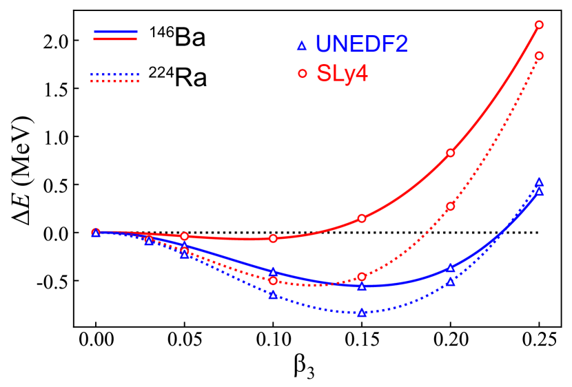
Figure 1: The deformation energies, $\Delta E(\beta_{3})=E(\beta_{3})-E(\beta_{3}=0)$, as functions of $\beta_{3}$ for ²²⁴Ra (dashed lines) and ¹⁴⁶Ba (solid lines) calculated at $\beta_{2}^{(0)}$ with the SLy4 (circles) and UNEDF2 (triangles) EDFs.

Figure 1 shows reflection-asymmetric deformation energies $\Delta E(\beta_{3})=E(\beta_{3})-E(\beta_{3}=0)$ determined for ²²⁴Ra and ¹⁴⁶Ba obtained in this way. We see that UNEDF2 gives a higher octupole deformability than SLy4 in both nuclei. This is consistent with the results of Ref. Cao et al. (2020).

IV.1 Multipole expansion of the deformation energy

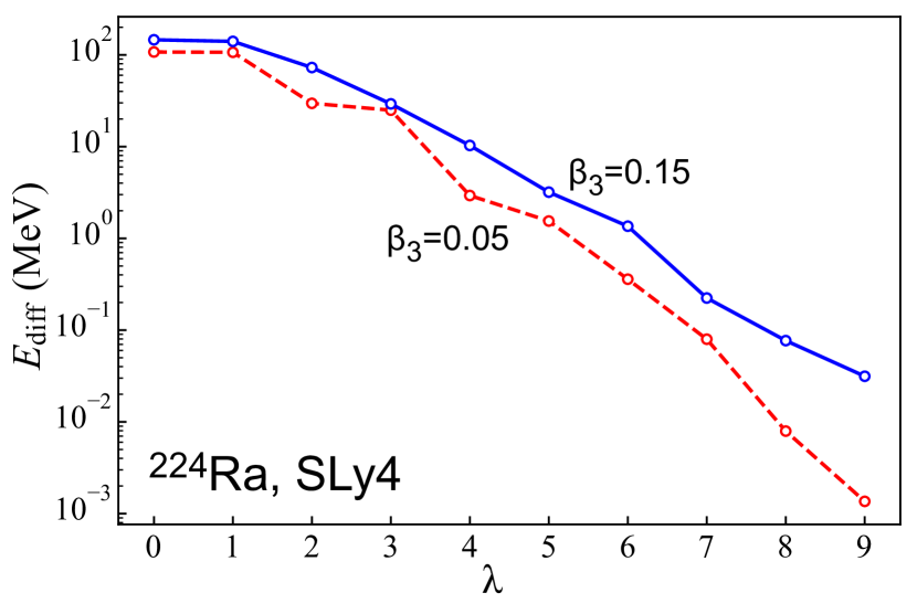
Figure 2: Convergence of $E_{\text{diff}}(\lambda)$ (36) for ²²⁴Ra computed with SLy4 at $\beta_{3}$=0.05 (dashed line) and 0.15 (solid line).

The convergence of the multipole expansion (15) provides a check on the accuracy of our results. In Fig. 2, we show the energy difference,

$$E_{\text{diff}}(\lambda)=\sum_{\lambda^{\prime}=0}^{\lambda}E_{[\lambda^{\prime}]}-E$$ (36)

for ²²⁴Ra at two values of the octupole deformation, $\beta_{3}=0.05$ and 0.15. We see that at $\beta_{3}=0.15$, the multipole components decrease exponentially with $\lambda$, with the monopole component off by about 150 MeV and the sum up to $\lambda=9$ exhausted up to about 20 keV. At a small octupole deformation of $\beta_{3}=0.05$, high-order contributions decrease. As expected, the octupole component brings now less energy as compared to the quadrupole one. The results displayed in Fig. 2 convince us that cutting the multipole expansion of energy at $\lambda=9$ provides sufficient accuracy.

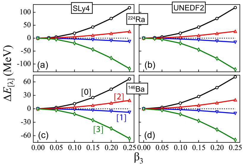
Figure 3: Multipole components, $\Delta E_{[\lambda]}(\beta_{3})=E_{[\lambda]}(\beta_{3})-E_{[\lambda]}(\beta_{3}=0)$, of the total deformation energy shown in Fig. 1, plotted for $\lambda=0-3$ as functions of the octupole deformation $\beta_{3}$ at $\beta_{2}^{(0)}$. Upper (lower) panels show results for ²²⁴Ra (¹⁴⁶Ba) obtained with the SLy4 (left) and UNEDF2 (right) EDFs.

Figure 3 shows how the reflection-asymmetric deformation energy builds up. It presents the four leading multipole components $\Delta E_{[\lambda]}(\beta_{3})=E_{[\lambda]}(\beta_{3})-E_{[\lambda]}(\beta_{3}=0)$, for $\lambda=0-3$, of the deformation energies shown in Fig. 1. We can see that the pattern of contributions of different multipolarities is fairly generic: it weakly depends on the choice of the nucleus or EDF. Figure 3 clearly demonstrates that the main driver of reflection-asymmetric shapes is a strong attractive octupole energy $\Delta E_{[3]}$. The attractive dipole energy $\Delta E_{[1]}$ is much weaker. The monopole and quadrupole energies are repulsive along the trajectory of $\beta_{3}$ (with a fixed quadrupole deformation $\beta_{2}^{(0)}$) and essentially cancel the octupole contribution. Indeed, one can note that while individual multipole components can be of the order of tens of MeV, the total reflection-asymmetric deformation energy shown in Fig. 1 is an order of magnitude smaller. Therefore, the final reflection-asymmetric correlation results from a large cancellation between individual multipole components, and even a relatively small variation of any given component can significantly shift the net result. In addition, as discussed in Sec. IV.3 below, higher-order multipole components ($\lambda>3$) can be important for the total energy balance.

IV.2 Isospin and neutron-proton structure of the octupole deformation energy

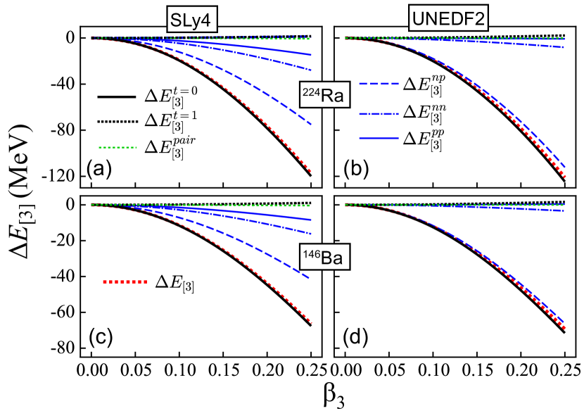
Figure 4: Similar to Fig. 3 but for different isospin and neutron-proton components of the octupole energy $\Delta E_{[3]}$.

To analyze the origin of the octupole energy $\Delta E_{[3]}$, in Fig. 4 we show its isospin and neutron-proton components as defined in Eqs. (31a) and (33). Again, a generic pattern emerges. In all cases, the octupole energy is almost equal to its isoscalar part $\Delta E^{t=0}_{[3]}$. The isovector energy $\Delta E^{t=1}_{[3]}$ is indeed very small, even if the studied nuclei have a significant neutron excess; this is consistent with the simple estimates of Sec. II. The contribution from the pairing energy $\Delta E^{\rm pair}_{[3]}$ is also practically negligible. In the neutron-proton scheme, the $np$ component always clearly dominates the $nn$ and $pp$ terms. The latter two are very small for UNEDF2 and hence $\Delta E_{[3]}\approx\Delta E^{t=0}_{[3]}\approx\Delta E^{np}_{[3]}$ for this EDF. For SLy4, the $nn$ and $pp$ terms provide larger contributions to the octupole deformation energy, accompanied by a reduction of the $np$ term. Regardless of these minor differences between the EDFs, we can safely conclude that it is the isoscalar octupole component (or the $np$ octupole energy component) that plays the dominant role in building up the nuclear octupole deformation.

IV.3 Reflection-asymmetric deformability along Isotopic chains

At this point, we are ready to study structural changes that dictate the appearance of nuclear reflection-asymmetric deformations. The results shown in Figs. 3 and 4 tell us that a mutual cancellation of near-parabolic shapes of different components of the deformation energy results in a clearly non-parabolic dependence of the total deformation energy, as seen in Fig. 1. Therefore, to track back the positions and energies of the equilibrium reflection-asymmetric deformations to the properties of specific interaction components is not easy. To this end, we analyze the properties of reflection-asymmetric deformabilities of nuclei, that is, we concentrate on the curvature of reflection-asymmetric deformation energies at $\beta_{3}=0$.

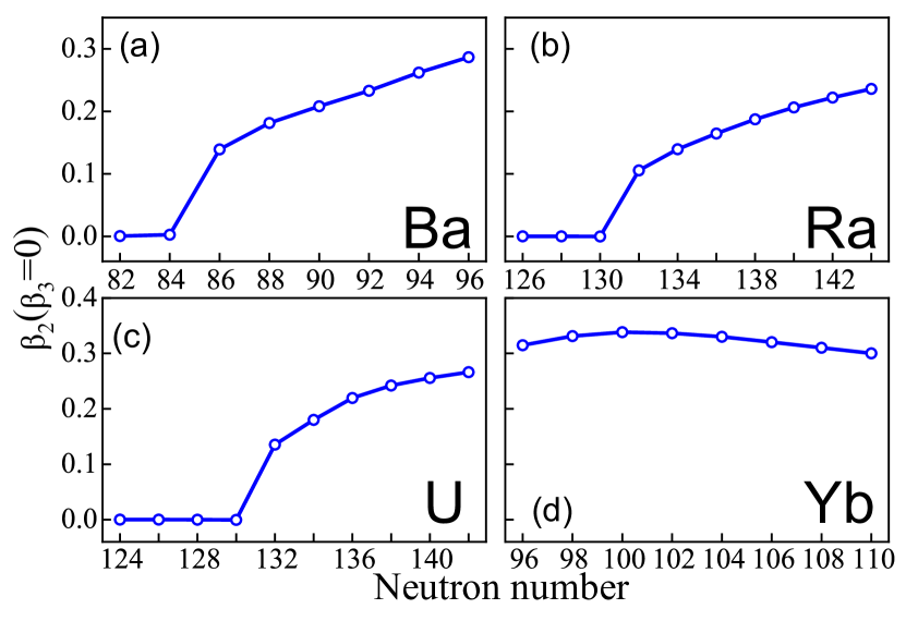
Figure 5: Equilibrium quadrupole deformations $\beta_{2}^{(0)}$ as functions of $N$ for the isotopic chains of (a) Ba, (b) Ra, (c) U, and (d) Yb computed with the SLy4 EDF.

To investigate the variation of the reflection-asymmetric deformability with neutron number, we performed SLy4-HFB calculations for the isotopic chains of even-even ^138-152Ba, ^214-232Ra, and ^216-234U isotopes, which are in the region of reflection-asymmetric instability, as well as ^166-180Yb, which are expected to be reflection-symmetric Cao et al. (2020). In Fig. 5 we show the baseline quadrupole deformations $\beta_{2}^{(0)}$. For the Ba, Ra, and U isotopic chains, spherical-to-deformed shape transitions are predicted slightly above the neutron magic numbers. The considered open-shell Yb isotopes are all predicted to be well deformed.

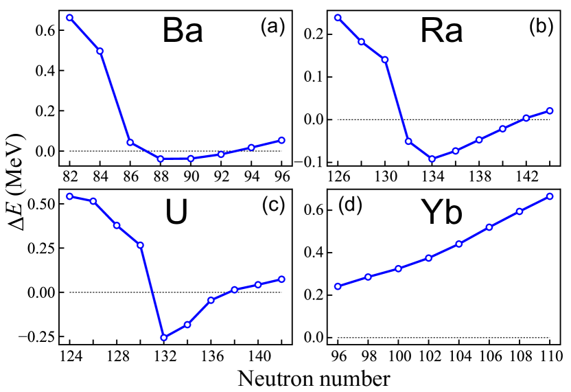
Figure 6: Similar to Fig. 5 but for the deformation energy $\Delta E=E(\beta_{3}=0.05)-E(\beta_{3}=0).$

As a quantitative measure of the octupole deformability, we analyze the deformation energy $\Delta E=E(\beta_{3}=0.05)-E(\beta_{3}=0)$ calculated at a small octupole deformation of $\beta_{3}=0.05$, with the quadrupole deformation fixed at $\beta_{2}^{(0)}$. We have checked that for different energy components, curvatures $\Delta E/\beta_{3}^{2}$ are stable within about 1% up to $\beta_{3}=0.05$, so values of $\Delta E$ taken at $\beta_{3}=0.05$ constitute valid measures of the octupole stiffness. In Fig. 6 we show the values of $\Delta E$ calculated for the four studied isotopic chains. We see that the negative values of $\Delta E$ delineate regions of neutron numbers where reflection-asymmetric deformations set in in Ba, Ra, and U isotopes Cao et al. (2020).

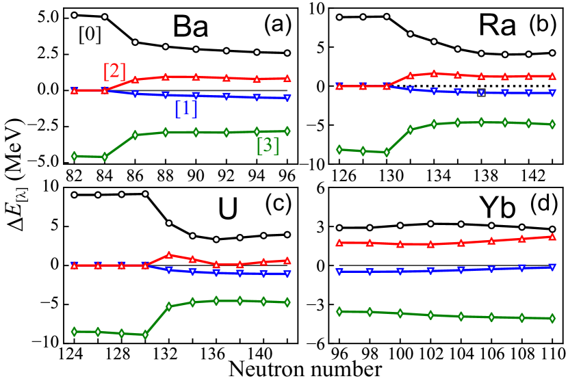
Figure 7: Similar to Fig. 5 but for the deformation energies $\Delta E_{[\lambda]}=E_{[\lambda]}(\beta_{3}=0.05)-E_{[\lambda]}(\beta_{3}=0)$ for $\lambda=0-3$.

We now study $\Delta E_{[\lambda]}$, the multipole components of the total deformation energy, for the four isotopic chains considered to see whether they could provide insights into the neutron-number dependence of octupole deformations. Figure 7 shows that the answer is far from obvious. Indeed, we observe strong cancellations of contributions coming from different multipole components of the reflection-asymmetric deformation energy. For example, both the repulsive monopole and attractive octupole components are an order of magnitude larger than the total deformation energies shown in Fig. 6. Therefore, we can expect that in order to understand the behavior of the deformation energies, higher-order multipole components $\Delta E_{[\lambda]}$ should be considered. Indeed, it has been early recognized that higher-order deformations can strongly influence the octupole collectivity of reflection-asymmetric nuclei Rozmej et al. (1988); Sobiczewski et al. (1988); Egido and Robledo (1989, 1990); Ćwiok and Nazarewicz (1989a, b, 1991); Nazarewicz (1992).

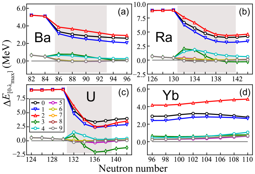
Figure 8: Similar to Fig. 7 but for the deformation energies $\Delta E=E(\beta_{3}=0.05)-E(\beta_{3}=0)$ with multipole components summed up from $\lambda=0$ to $\lambda_{\rm max}$. The values of $\lambda_{\rm max}$ are listed in the legend. The regions of deformed isotopes exhibiting reflection-asymmetric instability in Fig. 6 are marked by shading.

To better see accumulation effects with increasing multipolarity and subtle fluctuations at different orders, in Fig. 8 we plot multipole components of the octupole deformability summed up to $\lambda_{\rm max}$. Noting dramatically different scales of Figs. 6 and 8, we see that summations up to about $\lambda=5$ or 7 are needed for the results to converge. Although the octupole component contributes by far most to the creation of the reflection-asymmetric deformation energy, its effect is counterbalanced by a very large monopole component and, therefore, even higher multipole components are instrumental in determining the total reflection-asymmetric deformability. This aspect is underlined in the results shown in Figs. 9 and 10, where we separately show analogous sums of only odd-$\lambda$ (odd parity) and even-$\lambda$ (even parity) components, respectively. It is clear that the octupole polarizability is a result of a subtle balance between positive (repulsive) effect of the even-parity multipoles and negative (attractive) effect of the odd-parity multipoles.

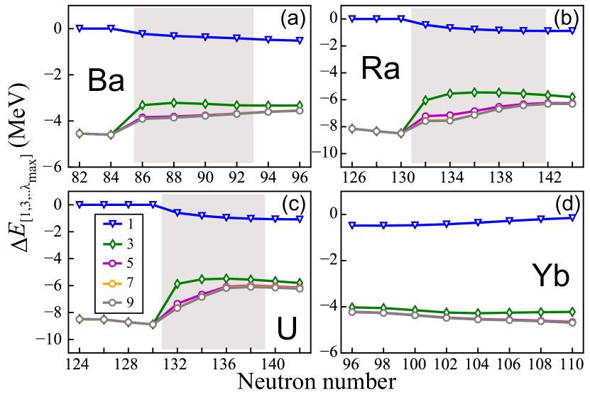
Figure 9: Similar to Fig. 8 but for the cumulative sum involving odd-$\lambda$ multipoles only.

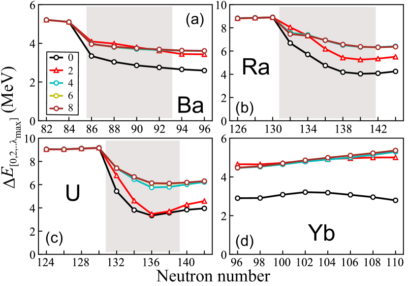
Figure 10: Similar to Fig. 8 but for the cumulative sum involving even-$\lambda$ multipoles only.

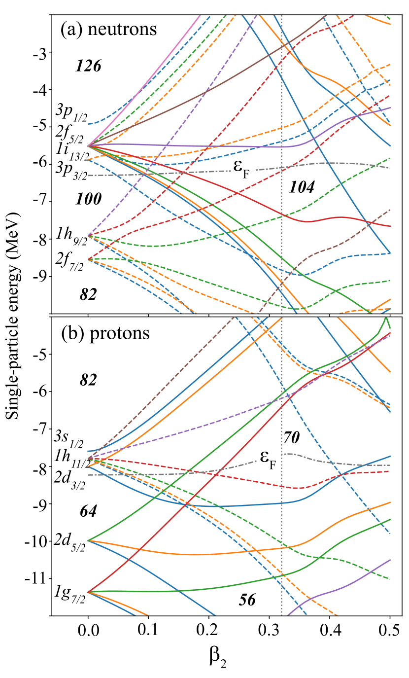
Figure 11: Single-particle (canonical) neutron (top) and proton (bottom) SLy4-HFB levels as functions of $\beta_{2}$ ($\beta_{3}=0$) for ¹⁷⁶Yb. Solid (dashed) lines indicate positive- (negative-) parity levels. Fermi levels $\varepsilon_{\rm F}$ at $N=106$ and $Z=70$ are marked by dash-dotted lines. The equilibrium deformation of ¹⁷⁶Yb is indicated by a vertical dotted line.

IV.4 Relation to shell structure

To gain some insights into the shell effects behind the appearance of stable reflection-asymmetric nuclear shapes, Figs. 11 and 12 show, respectively, the s.p. level diagrams for ¹⁷⁶Yb and ²²⁴Ra as functions of $\beta_{2}$. While such diagrams cannot predict symmetry breaking effects per se, they can often provide qualitative understanding.

The well-deformed nucleus ¹⁷⁶Yb is characteristic of a stiff octupole vibrator. Indeed, its nucleon numbers ($Z=70,N=106$) lie far from the “octupole-driving” numbers $N_{\rm oct}$. Due to the large deformed $Z=70$ gap around $\beta_{2}=0.32$, there are no s.p. states of opposite parity and the same projection $\Omega$ of the total s.p. angular momentum on the symmetry axis that could produce p-h excitations with appreciable $\lambda=3$ strength across the Fermi level. As for the neutron s.p. levels, the low-$\Omega$ positive-parity states originating from the $1i_{13/2}$ shell lie below the Fermi level, which appreciably reduces the $1i_{13/2}\leftrightarrow 2f_{7/2}$ strength. Because of the large quadrupole deformations of Yb isotopes considered, the s.p. orbital angular momentum $\ell$ of normal-parity orbitals is fairly fragmented within the shell Bengtsson et al. (1989). As seen in Figs. 10d and 9d, all multipole components of $\Delta E$ for ¹⁷⁶Yb vary very smoothly with neutron number.

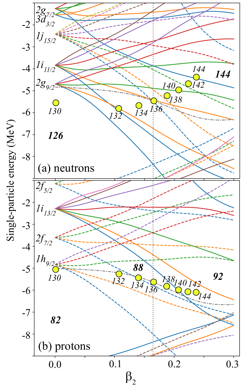
Figure 12: Similar to Fig. 11 but for ²²⁴Ra. Fermi levels for even-even Ra isotopes with $N=130-144$ are marked by circles. They have been shifted according to the position of the spherical $2g_{9/2}$ neutron and $1h_{9/2}$ proton shell. The equilibrium deformation of ²²⁴Ra is indicated by a vertical dotted line.

The Nilsson diagram shown in Fig. 12 is characteristic of transitional neutron-deficient actinides in which the octupole instability is expected. The unique-parity shells, $1i_{13/2}$ proton shell and $1j_{15/2}$ neutron shell, are of particle character, which results in an appearance of close-lying opposite-parity pairs of Nilsson levels with the same low $\Omega$-values at intermediate quadrupole deformations. These levels can interact via the octupole field, with the dominant $\pi 1i_{13/2}\leftrightarrow\pi 2f_{7/2}$ and $\nu 1j_{15/2}\leftrightarrow\nu 2g_{9/2}$ couplings.

As seen in Figs. 9 and 10, in the regions of octupole instability, the monopole and quadrupole deformation energies become locally reduced while the octupole and dotriacontapole ($\lambda=5$) contributions to $\Delta E$ grow. According to our results, the effect of the dotriacontapole term is essential for lowering $\Delta E$ around $N_{\rm oct}$. This not surprising as the main contribution to the dotriacontapole coupling comes from the $\Delta\ell=\Delta j=3$ excitations Ćwiok and Nazarewicz (1989a, 1991), i.e., the octupole and dotriacontapole correlations are driven by the same shell-model orbits. Interestingly, it is the attractive $\lambda=5$ contribution to $\Delta E$ rather than the octupole term that exhibits the local enhancement in the regions of octupole instability.

The shallow octupole minima predicted around ¹⁴⁶Ba result from an interplay between the odd-$\lambda$ deformation energies, which gradually increase with $N$ (see Fig. 9a) and the even-$\lambda$ deformation energies, which gradually decrease with $N$ (see Fig. 10b). Again, the dotriacontapole moment is absolutely essential for forming the octupole instability.

V Conclusions

In this work, we used the Skyrme-HFB approach to study the multipole expansion of interaction energies in both isospin and neutron-proton schemes in order to analyze their role in the appearance of reflection-asymmetric g.s. deformations. The main conclusions and results of our study can be summarized as follows:

1. Based on the self-consistent HFB theory, reflection-asymmetric ground-state shapes of atomic nuclei are driven by the odd-multipolarity isoscalar (or, in neutron-proton scheme, $np$) part of the nuclear interaction energy. In a simple particle-vibration picture, this can be explained in terms of the very large isoscalar octupole polarizability $\chi_{3,0}(\Delta{\cal N}=1)=3$.

2. The most favorable conditions for reflection-asymmetric shapes are in the regions of transitional nuclei with neutron and proton numbers just above magic numbers. For such systems, the unique-parity shell has a particle character, which creates favorable conditions for the enhanced $\Delta\ell=\Delta j=3$ octupole and dotriacontapole couplings.

3. The presence of high-multipolarity interaction components, especially $\lambda=5$ are crucial for the emergence of stable reflection-asymmetric shapes. Microscopically, dotriacontapole couplings primarily come from the same $\Delta\ell=\Delta j=3$ p-h excitations that are responsible for octupole instability. According to our calculations, the attractive $\lambda=5$ contribution to the octupole stiffness is locally enhanced in the regions of reflection-asymmetric g.s. shapes.

In summary, stable pear-like g.s. shapes of atomic nuclei result from a dramatic cancellation between even- and odd-multipolarity components of the nuclear binding energy. Small variations in these components, associated, e.g., with the s.p. shell structure, can thus be instrumental for tilting the final energy balance towards or away from the octupole instability. One has to bear in mind, however, that the shell effect responsible for the spontaneous breaking of intrinsic parity is weak, as it is associated with the appearance of isolated $\Delta\ell=\Delta j=3$ pairs of levels (parity doublets) in the reflection-symmetric s.p. spectrum. In this respect, the breaking of the intrinsic spherical symmetry in atomic nuclei (presence of ellipsoidal deformations) is very common as every spherical s.p. shell (except for those with $j=1/2$) carries an intrinsic quadrupole moment that can contribute to the vibronic coupling.