Abstract

We establish selection of critical pulled fronts in invasion processes as predicted by the marginal stability conjecture. Our result shows convergence to a pulled front with a logarithmic shift for open sets of steep initial data, including one-sided compactly supported initial conditions. We rely on robust, conceptual assumptions, namely existence and marginal spectral stability of a front traveling at the linear spreading speed and demonstrate that the assumptions hold for open classes of spatially extended systems. Previous results relied on comparison principles or probabilistic tools with implied non-open conditions on initial data and structure of the equation. Technically, we describe the invasion process through the interaction of a Gaussian leading edge with the pulled front in the wake. Key ingredients are sharp linear decay estimates to control errors in the nonlinear matching and corrections from initial data.

1 Introduction

The onset of structure formation in spatially extended physical systems is often mediated by an invasion process, in which a pointwise stable state invades a pointwise unstable state. One observes that an initially localized perturbation to the pointwise unstable background state grows in amplitude and spreads spatially. In its wake, this spreading process may select a spatially constant state, a periodic pattern, or more complicated dynamics; see [84] for a thorough review of experimental observations of invasion processes across the sciences. The fundamental objective then is to describe this process, in particular by predicting the spreading speed and the selected state in the wake.

A mathematical study usually focuses first on a one-sided invasion process, describing convergence of solutions to a front that connects the unstable state in the leading edge to the selected state in the wake. Existence of such fronts and stability information is often available through a variety of analytical and computational techniques, ranging from comparison methods and monotonicity [27, 87] to integrability [63, 85], to perturbative techniques in small-amplitude settings [15, 16, 20, 23, 45, 72] or in the presence of scale separation [14, 32, 75], to topological techniques [79, 80] and to rigorous computational approaches [6]; see also the review [84]. The marginal stability conjecture connects such existence and stability information with the physically most interesting question as to which fronts are actually selected, that is, observed when starting from steep, particularly compactly supported initial conditions; see for instance [18, 15, 84]. In essence, the conjecture predicts that out of a family of fronts, the “marginally stable” front is selected and thus reduces, whenever proven, the study of invasion processes to the study of existence and stability of front solutions. Our work here makes this concept of marginal stability precise and establishes the conjecture.

Linear marginal stability. Motivating this conjecture are predictions based on the linearized problem at the trivial unstable state. Spatially localized disturbances in this linearized problem grow exponentially and spread spatially. Analyzing stability in comoving frames of speed $c$, one finds that perturbations exhibit pointwise exponential decay for all speeds above a critical speed, $c>c_{*}$. The pointwise decay or growth is typically encoded in the complex linear dispersion relation through pinched double roots $\lambda_{\mathrm{dr}}(c)$: one finds pointwise exponential behavior $\sim\exp(\lambda_{\mathrm{dr}}t)$ with $\mathrm{Re}\,\lambda_{\mathrm{dr}}(c)<0$ for $c>c_{*}$ and marginal stability $\mathrm{Re}\,\lambda_{\mathrm{dr}}(c_{*})=0$ at the “critical” linear spreading speed $c_{*}$ [8, 13, 49]; see Section 1.2 for a brief review. In addition to predictions for the speed, the linear analysis also offers a prediction for the nature of the invasion process: zero versus nonzero frequency $\mathrm{Im}\,\lambda_{\mathrm{dr}}(c_{*})$ predicts invasion that is

(S) stationary  or  (P) time-periodic.

in the comoving frame.

Nonlinear stability. Nonlinear saturation of this linear growth process leads to formation of fronts. Describing the evolution towards fronts, one invokes subtle stability arguments. Pointwise stability is mostly intractable in nonlinear equations, and one therefore resorts to function spaces with exponential weights, penalizing in particular perturbations in the leading edge of the front that would grow due to the inherent instability of the invaded state. In the leading edge, the linearized evolution is indeed close to the linearization at the unstable state and one finds that fronts with speeds $c<c_{*}$ are unstable in any weighted space. Fronts with speed $c\geq c_{*}$ however can often be shown to be stable in exponentially weighted spaces, based on properties of the linearization at the front. One therefore analyzes the spectrum of the linearization, which is composed of essential spectrum related to stability in the leading edge, essential spectrum related to stability in the wake, and point spectrum associated with stability of the front interface. In suitably weighted spaces, one establishes or assumes that essential spectrum associated with the leading edge is stable for $c>c_{*}$ and marginally stable for $c=c_{*}$, while point spectrum and essential spectrum associated with the state in the wake are stable or marginally stable; see also Figure 1.

This perspective recovers some notion of stability but does not address the question of speed selection, since all fronts with speeds $c\geq c_{*}$ are stable in this sense. It turns out that permissible perturbations of the front in such stability arguments are very localized so that initial conditions given by the sum of front and perturbation necessarily preserve the exponential decay rate in the leading edge of the front. The arguments do in particular not describe the behavior of the most relevant steep, for instance step-function like, initial conditions.

The marginal stability conjecture. The marginal stability conjecture states that, nevertheless, information on the existence and stability of fronts does yield a selection criterion:

Marginally stable fronts are selected by steep initial conditions.

The hypothesis is understood to hold universally across equations for open classes of steep initial conditions, under appropriate notions of marginal stability; see [84, 18, 23, 24] for statements of the conjecture in many specific examples. In this paper, we will define marginal stability through spectral properties of the linearization of the front in norms with exponentially growing weights in the leading edge, encoding marginal stability in the leading edge, absence of unstable or marginally stable spectrum associated with the front interface or the wake; see Hypotheses 1–4, below. Fronts where marginal stability is caused by the leading edge are commonly referred to as pulled fronts. In that regard, our assumptions exclude pushed fronts, with instability in the front interface, and staged invasion with instabilities in the wake. Selection of pushed fronts is easier to establish than that of pulled fronts, since for pushed fronts a spectral gap may be recovered with exponential weights; see Section 8 for a discussion of pushed fronts and other secondary instability mechanisms. We define selection in Definition 1 as allowing for open classes of steep initial conditions. Our main result, precisely stated in Theorem 1, establishes the marginal stability conjecture under these conceptual assumptions.

Theorem.

The marginal stability conjecture holds in the case (S) of stationary invasion assuming existence of a rigidly propagating (marginally stable) pulled front, that is, open classes of steep initial conditions converge to an appropiately shifted front profile with speed $c_{*}$.

In addition, we address the universality aspect of the marginal stability conjecture in Theorem 2, which shows that our assumptions hold for open classes of equations. Contrasted with previous work, our result does not rely on the structure of the equation or sign conditions on initial data. We rephrase the front selection problem as a stability problem for fronts similar to [33, 26, 4, 24], but, crucially, with supercritical localization of perturbations to the front. In fact, as we shall see later, dynamics near a critical front profile exhibit diffusive decay in suitable norms for localized perturbations of the front. However, again in suitable norms, steep initial data induces perturbations of fronts that grow linearly in the leading edge and therefore do not decay diffusively. In this respect, our results can be compared to efforts toward establishing diffusive decay in pattern-forming systems, where neutral modes decay diffusively, and where modulation equations attempt to capture dynamics when perturbations are not spatially localized [21, 34, 52, 54, 55, 56, 77].

A brief history and examples. Specific to front selection, the mathematical literature originates with work in the 1930s on the Fisher-KPP equation [31, 61],

$$\partial_{t}u=\partial_{xx}u+u-u^{2},\quad x\in\mathbb{R},\quad t>0,$$ (1.1)

where fronts connecting the stable state $u\equiv 1$ to the unstable state $u\equiv 0$ are linearly stable for speeds $c\geq 2$, the linear spreading speed. Kolmogorov, Petrovskii, and Piskunov [61] proved in 1937 that for step function initial data, $u=1,x<0$ and $u=0$, $x>0$, the solution to (1.1) indeed converges to shifted pulled fronts,

$$\lim_{t\to\infty}u(x+\sigma(t),t)=q(x;2),$$ (1.2)

for some shift $\sigma(t)=2t+\mathrm{o}(t)$, uniformly in space, where $q(\cdot;2)$ is a front solution to (1.1) satisfying $u(x,t)=q(x-2t;2)$, unique up to spatial translation. In particular, the speed $\sigma^{\prime}(t)=2+\mathrm{o}(1)$ converges to the linear spreading speed as $t\to\infty$. The basic idea of the proof relies on using comparison principles, with (unstable) fronts at speeds $c\lesssim 2$ as subsolution building blocks, and was subsequently adapted to a plethora of systems that allow comparison principles, sometimes in a more hidden fashion, on the real line and also in higher space dimensions; see e.g. [2, 7, 40, 42, 73, 87]. In a celebrated series of papers, Bramson [11, 12] showed that convergence of the speed is quite slow with a universal leading-order correction that induces a $\log$-shift in the position, independent of initial conditions,

$$\sigma(t)=2t-\frac{3}{2}\log t+\mathrm{O}(1).$$ (1.3)

The approach there relies on a probabilistic interpretation of (1.1) as an evolution of distributions in a branched random walk. Proofs were greatly simplified later using comparison principles with refined subsolutions in [62, 41, 66]. The new techniques introduced also led to refined asymptotics, allowed adaptations to other systems, and analysis in higher space dimensions; see e.g. [67, 38, 10, 9, 74].

Inspecting the comprehensive review of experimental observations and theoretical studies of front propagation into unstable states [84], almost all experimental settings and associated models including for instance fluid instabilities, crystal growth, and phase separation, do not admit a probabilistic interpretation or comparison principles, nor do they preserve positivity of initial data. In fact key examples in [84] are higher-order parabolic equations that do not admit comparison principles. A prototypical case of stationary propagation (S) is the extended Fisher-KPP equation

$$\partial_{t}u=-\delta^{2}\partial_{xxxx}u+\partial_{xx}u+f(u),\quad x\in\mathbb{R},\quad t>0,$$ (1.4)

for $\delta$ small, where $f$ is a smooth function satisfying $f(0)=f(1)=0$, $f^{\prime}(0)>0,f^{\prime}(1)<0$, and (for instance) $f^{\prime\prime}(u)<0$ for all $u\in(0,1)$. A basic example for time-periodic propagation, case (P), is the Swift-Hohenberg equation, a prototypical model for pattern formation in contexts such as Rayleigh-Bénard convection,

$$\partial_{t}u=-\partial_{xxxx}u-2\partial_{xx}u+(\mu-1)u-u^{3},\quad x\in\mathbb{R},\quad t>0,\quad\mu>0;$$ (1.5)

see [23] for a formulation of the marginal stability conjecture in this particular case. Fourth order (and even sixth) order scalar equations such as (1.4) and (1.5) arise in many physical circumstances, including in phenomenological models for convection rolls [82], in crystal nucleation and growth [25, 86], in models for spatial localization of patterns across many physical systems [60], as models for phyllotaxis [70], as amplitude equations derived from reaction-diffusion or fluid systems [65, 76], and even in Turing’s late work on morphogenesis [17].

Motivated by these examples, we focus on a setting of higher-order parabolic equations in which we establish selection of pulled fronts and the marginal stability conjecture in the case of stationary invasion (S). We believe that the techniques introduced here will also prove useful in understanding front propagation in the time-periodic case (P), particularly in pattern-forming systems such as (1.5). We further expect the linear theory which we develop here and in [4] to be useful in understanding diffusive decay near coherent structures in other contexts.

1.1 Setup and main results

We consider scalar, spatially homogeneous parabolic equations of arbitrary order, of the form

$$u_{t}=\mathcal{P}(\partial_{x})u+f(u),\quad u=u(x,t)\in\mathbb{R},\quad x\in\mathbb{R},\quad t>0,$$ (1.6)

with $f$ smooth, $f(0)=f(1)=0,f^{\prime}(0)>0$, and $f^{\prime}(1)<0$, and polynomial differential operator

$$\mathcal{P}(\nu)=\sum_{k=0}^{2m}p_{k}\nu^{k},\quad(-1)^{m}p_{2m}<0,\quad p_{0}=0,$$ (1.7)

so that $\mathcal{P}(\partial_{x})$ is elliptic of order $2m$, although not necessarily symmetric, that is, we allow nonzero coefficients of odd derivatives.

We pass to a comoving frame of speed $c$ and linearize at the unstable rest state $u\equiv 0$ to find

$$u_{t}=\mathcal{P}(\partial_{x})u+c\partial_{x}u+f^{\prime}(0)u.$$ (1.8)

Informally, the linear spreading speed $c_{*}$ is a distinguished speed so that solutions to (1.8) with compactly supported initial data grow exponentially pointwise for $c\lesssim c_{*}$ and decay pointwise for $c\gtrsim c_{*}$. To characterize $c_{*}$, we substitute $u=e^{\nu x+\lambda t}$ into (1.8) and find the dispersion relation,

$$d^{+}_{c}(\lambda,\nu):=\mathcal{P}(\nu)+c\nu+f^{\prime}(0)-\lambda.$$ (1.9)

The dispersion relation determines the spectrum of the linearization about the unstable state $\mathcal{P}(\partial_{x})+c_{*}\partial_{x}+f^{\prime}(0)$ via the Fourier transform, in the sense that the spectrum of this operator (on, for instance, $L^{p}(\mathbb{R})$) is given by

$$\Sigma^{+}=\{\lambda\in\mathbb{C}:d^{+}(\lambda,ik)=0\text{ for some }k\in\mathbb{R}\}.$$ (1.10)

Hypothesis 1 (Linear spreading speed).

We assume there exists a speed $c_{*}$ and an exponential rate $\eta_{*}>0$ such that

• (Simple pinched double root) For $\nu,\lambda$ near 0, we have for some $\alpha>0$,

  $$d^{+}_{c_{*}}(\lambda,\nu-\eta_{*})=\alpha\nu^{2}-\lambda+\mathrm{O}(\nu^{3});$$ (1.11)

• (Minimal critical spectrum) If $d^{+}_{c_{*}}(i\kappa,ik-\eta_{*})=0$ for some $k,\kappa\in\mathbb{R}$, then $k=\kappa=0$;

• (No unstable spectrum) $d^{+}_{c_{*}}(\lambda,ik-\eta_{*})\neq 0$ for any $k\in\mathbb{R}$ and any $\lambda\in\mathbb{C}$ with $\mathrm{Re}\,\lambda>0$.

Remark 1.1.

Hypothesis 1 implies that a transition from pointwise growth to pointwise decay occurs at $c=c_{*}$. The rate $\eta_{*}$ naturally arises in this stability computation, and characterizes both the exponential decay rate of pulled fronts and the natural choice of an exponentially weighted space for perturbations. Indeed, assumption (i) implies by Fourier transform in $x$ that, in a space with weight $e^{\eta_{*}x}$, the essential spectrum of the linearization about $u\equiv 0$ has a branch that touches the imaginary axis at the origin and is otherwise contained in the left half plane (see Figure 1). It is then natural to assume that the essential spectrum is otherwise stable, which is captured in (ii) and (iii), so that dynamics are governed by the marginal pointwise stability captured by the simple pinched double root criterion. On the other hand, choosing $\mathrm{Re}\,\nu\neq 0$, small in (1.11) shows that the origin is unstable in weights $\eta\approx\eta_{*}$, $\eta\neq\eta_{*}$. Using (ii) and (iii) one can show that instability holds for all weights $\eta\neq\eta_{*}$. Similarly, for speeds $c>c_{*}$, we have $\mathrm{Re}\,\lambda\leq\delta<0$ when $\mathrm{Re}\,\nu=-\eta_{*}$, implying exponential decay of perturbations in a weighted norm, while for speeds $c<c_{*}$, one finds $\mathrm{Re}\,\lambda>0$ for some $\nu\in-\eta+i\mathbb{R}$, for any $\eta$ fixed; see Section 1.2 for further details. It is in this sense that Hypothesis 1 specifies marginal stability at speed $c_{*}$.

From now on we fix $c=c_{*}$ and write $d^{+}=d^{+}_{c_{*}}$. We also define the left dispersion relation

$$d^{-}(\lambda,\nu)=\mathcal{P}(\nu)+c_{*}\nu+f^{\prime}(1)-\lambda$$ (1.12)

which determines the spectrum of the linearization $\mathcal{P}(\partial_{x})+c_{*}\partial_{x}+f^{\prime}(1)$ at $u=1$ through

$$\Sigma^{-}=\{\lambda\in\mathbb{C}:d^{-}(\lambda,ik)=0\text{ for some }k\in\mathbb{R}\}.$$ (1.13)

We focus on dynamics in the leading edge and therefore assume (strict) stability in the wake.

Hypothesis 2 (Stability in the wake).

We assume that $\mathrm{Re}\,(\Sigma^{-})<0$.

According to the marginal stability conjecture, one expects the propagation dynamics to be governed by traveling wave solutions, and we therefore assume existence of such a front.

Hypothesis 3 (Existence of a critical front).

We assume there exists a solution to (1.6) of the form

$$u(x,t)=q_{*}(x-c_{*}t),\qquad\lim_{\xi\to-\infty}q_{*}(\xi)=1,\quad\lim_{\xi\to\infty}q_{*}(\xi)=0.$$ (1.14)

We refer to $q_{*}$ as the critical front. Moreover, we assume that for some $a,b\in\mathbb{R}$ with $b\neq 0$ and some $\eta_{0}>0$,

$$q_{*}(\xi)=(a+b\xi)e^{-\eta_{*}\xi}+\mathrm{O}(e^{-(\eta_{*}+\eta_{0})\xi}).$$ (1.15)

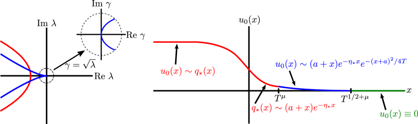
Figure 1: Left: the Fredholm borders of $\mathcal{L}$ associated to the asymptotic operators on the right (blue, marginally stable) and on the left (red, stable), together with inset showing an image of the origin under the map $\lambda\mapsto\sqrt{\lambda}$. The Fredholm borders determine the boundary of the essential spectrum; see Section 3 for details. Right: schematic of a representative initial datum $u_{0}$ to which our selection result applies.

Possibly translating in space and reflecting $q_{*}\mapsto-q_{*}$ if necessary, we assume $b=1$.

Remark 1.2.

The assumption (1.15) on the asymptotics of the critical front is generic for pulled fronts. Writing the traveling wave ODE as a first-order system, the front connects two equilibria. Eigenvalues at the linearization at $u=0$ are roots of $d_{c_{*}}^{+}(0,\nu)=0$. Homotoping from $\lambda=0$ to $\lambda=+\infty$, we notice that roots $\nu$ do not cross $\mathrm{Re}\,\nu=-\eta_{*}$ by (iii). Using (1.11), one quickly concludes that the linearization at the origin has $m-1$ eigenvalues with real part less than $-\eta_{*}$, and a Jordan block of length 2 at $-\eta_{*}$. ODE theory shows that solutions with decay at most $e^{-\eta_{*}x}$ then form a smooth $m$-dimensional strong stable manifold, solutions with decay at most $xe^{-\eta_{*}x}$ form a smooth $m+1$-dimensional strong stable manifold. Similarly, the equilibrium corresponding to $u=1$ is hyperbolic and possesses an $m$-dimensional unstable manifold. Counting dimensions, we find generically a discrete set of heteroclinic orbits with decay rate $xe^{-\eta_{*}x}$ but no solutions with decay $e^{-\eta_{*}x}$, confirming the asymptotics (1.15) in a generic situation.

Finally, we need to exclude the possibility that the fronts are pushed in the sense that the nonlinearity accelerates the speed of propagation. Typically, in the presence of pushed fronts, the linearization about the critical front has an unstable eigenvalue. This linearization is given by

$$\mathcal{A}=\mathcal{P}(\partial_{x})+c\partial_{x}+f^{\prime}(q_{*}).$$ (1.16)

The assumption $f^{\prime}(0)>0$ implies that the essential spectrum of $\mathcal{A}$ on $L^{2}$ is unstable [30, 68, 69], but Hypotheses 1 and 2 imply that, with a smooth positive exponential weight $\omega$ satisfying

$$\omega(x)=\begin{cases}e^{\eta_{*}x},&x\geq 1,\\ 1,&x\leq-1,\end{cases}$$ (1.17)

the essential spectrum of the conjugate operator $\mathcal{L}=\omega\mathcal{A}\omega^{-1}$ is marginally stable; see Figure 1 for a schematic, and the beginning of Section 3 for further details. To exclude pushed fronts, we assume the following.

Hypothesis 4 (No resonance or unstable point spectrum).

We assume that $\mathcal{L}:H^{2m}(\mathbb{R})\subset L^{2}(\mathbb{R})\to L^{2}(\mathbb{R})$ does not have any eigenvalues $\lambda$ with $\mathrm{Re}\,\lambda\geq 0$. We further assume that there is no bounded solution to $\mathcal{L}u=0$.

In the Fisher-KPP setting, fronts with the linear spreading speed $c=2$ satisfy Hypotheses 1–4. Absence of a bounded solution to $\mathcal{L}u=0$ in the Fisher-KPP equation is a consequence of the weak exponential decay (1.15) of the critical front. Instabilities as excluded in Hypothesis 4 occur for instance when considering an asymmetric cubic nonlinearity and lead to the selection of pushed fronts that propagate at a speed $c_{\mathrm{pushed}}>c_{*}$; see [39]. Separating pulled fronts with speed $c=2$ from pushed fronts is the case of of a bounded solution to $\mathcal{L}u=0$, excluded in Hypothesis 4. In the case that there is such a bounded solution, we say $\lambda=0$ is a resonance of $\mathcal{L}$.

Before we can state our main results, we address the question: what features should a meaningful front selection result have? First, such a result should establish that, for an open class of initial data, the front interface is located approximately at $x=c_{*}t$ for large times, so that the asymptotic speed of propagation is the linear spreading speed. Second, the class of initial data should include some data that is compactly supported in the leading edge, commonly the most interesting case. Such a setting rules out selection in this sense of faster-traveling, supercritical fronts [22], $c>c_{*}$, which attract open sets of initial data but only with well-prepared, slowly decaying exponential tails.

Definition 1.

We say that a front $q_{*}$ with speed $c_{*}$ in (1.6) is a selected front if an open class of steep initial conditions propagates with asymptotic speed $c_{*}$ and stays close to translates of the front $q_{*}$. More precisely, we require that there exists a non-negative continuous weight $\rho:\mathbb{R}\to\mathbb{R}$ and, for any $\varepsilon>0$, a set of initial data $\mathcal{U}_{\varepsilon}\subseteq L^{\infty}(\mathbb{R})$ such that:

• for any $u_{0}\in\mathcal{U}_{\varepsilon}$, there exists a function $h(t)=\mathrm{o}(t)$ such that the solution $u(x,t)$ to (1.6) with initial data $u_{0}$ satisfies, for $t$ sufficiently large,

  $$\|u(\cdot+c_{*}t+h(t),t)-q_{*}(\cdot)\|_{L^{\infty}(\mathbb{R})}<\varepsilon;$$ (1.18)

• there exists $u_{0}\in\mathcal{U}_{\varepsilon}$ such that $u_{0}(x)=0$ for all $x>0$ sufficiently large;

• $\mathcal{U}_{\varepsilon}$ is open in the topology induced by the norm $\|g\|_{\rho}=\|\rho g\|_{L^{\infty}}$.

Our result includes a specific choice of algebraic weight with smooth, positive weight function $\rho_{r}$, $r\in\mathbb{R}$, satisfying

$$\rho_{r}(x)=\begin{cases}\langle x\rangle^{r},&x\geq 1,\\ 1,&x\leq-1,\end{cases}$$ (1.19)

where $\langle x\rangle=(1+x^{2})^{1/2}$.

Theorem 1.

Assume Hypotheses 1 through 4 hold. Then the critical front $q_{*}$ with speed $c_{*}$ is a selected front, with weight $\rho=\rho_{r}\omega$ for $r=2+\mu$, $0<\mu<\frac{1}{8}$. Furthermore, for each $\varepsilon>0$ small there exists $\mathcal{U}_{\varepsilon}\subseteq L^{\infty}(\mathbb{R})$ satisfying Definition 1, (ii)–(iii), such that the refined estimate

$$\sup_{x\in\mathbb{R}}|\rho_{-1}(x)\omega(x)[u(x+\sigma(t),t)-q_{*}(x)]|<\varepsilon$$ (1.20)

holds for solutions with initial data $u_{0}\in\mathcal{U}_{\varepsilon}$ and $t\geq t_{*}(u_{0})$, sufficiently large, where, for some $x_{\infty}(u_{0})$,

$$\sigma(t)=c_{*}t-\frac{3}{2\eta_{*}}\log t+x_{\infty}(u_{0}).$$ (1.21)

Remark 1.3.

In addition to universal selection of pulled fronts, Theorem 1 establishes universality of the logarithmic delay $-\frac{3}{2\eta_{*}}\log t$ as identified by Ebert and van Saarloos [22]: the delay is present in all equations satisfying our conceptual assumptions and is independent of the initial data. The matched asymptotics in [84] suggest that there are further universal terms in the expansion of the position of the front: in particular, $u(x+\tilde{\sigma}(t),t)\to q_{*}(x)$, where

$$\tilde{\sigma}(t)=c_{*}t-\frac{3}{2\eta_{*}}\log t+\tilde{x}_{\infty}+\frac{\sigma_{2}}{\sqrt{t}}+\mathrm{o}(t^{-1/2})$$

for a constant $\sigma_{2}$ with explicit, universal form depending only on the leading order expansion of the dispersion relation. Such expansions, including to higher orders, have been verified for the Fisher-KPP equation in [67, 38]. We do not pursue such higher expansions in the more general setting here, instead focusing on the most relevant questions of selection of the speed and the state in the wake.

We emphasize that we do not require any structure of the equation beyond Hypotheses 1 through 4 — in particular, our results apply to equations without comparison principles. The first author together with Garénaux recently proved [3] that the extended Fisher-KPP equation (1.4) satisfies Hypotheses 1 through 4, so that Theorem 1 applies immediately in that setting. Adapting the ideas therein, we show that the class of equations we consider here is open, thereby emphasizing the universality across different equations. We make this precise in the following theorem.

Theorem 2.

Assume that $\mathcal{P}(\partial_{x};\delta)$ is a family of operators of degree $2m$ of the form (1.7) for $\delta\in(-\delta_{0},\delta_{0})$ for some $\delta_{0}>0$, with coefficients $p_{k}(\delta)$ smooth in $\delta$, $p_{2m}(0)\neq 0$, and that $f=f(u;\delta)$ is smooth in both $u$ and $\delta$. Suppose that $f(0;0)=f(1;0)=0,$ $f^{\prime}(0;0)>0,f^{\prime}(1;0)<0$, and $\mathcal{P}(\partial_{x};0)$ and $f(u;0)$ are such that Hypotheses 1 through 4 are satisfied. Assume further that $f(0;\delta)=f(1;\delta)=0$. Then Hypotheses 1 through 4 also hold for $\delta$ sufficiently small, and hence Theorem 1 holds for all $\delta$ sufficiently small.

We note in passing that the assumptions in Theorem 2 on the nonlinearity at $\delta=0$ imply that $0$ and $1$ perturb smoothly to nearby zeros of $f$ for $\delta$ small. Shifting and rescaling $u$, we may then assume without loss of generality that $f(0;\delta)=f(1;\delta)=0$.

Together, Theorems 1 and 2 establish propagation at the linear spreading speed for open classes of initial data and open classes of equations.

1.2 Overview and preliminaries

Pointwise stability and pinched double roots. We give a brief review of concepts of pointwise decay driving our understanding of invasion processes, and the role of pinched double roots, based on the presentation in [49]. To determine pointwise growth or decay for solutions to the linearization about the unstable state, we use the inverse Laplace transform to write the solution to (1.8) as

$$u(x,t)=\frac{1}{2\pi i}\int_{\Gamma}e^{\lambda t}\int_{\mathbb{R}}G_{\lambda}(x-y)u_{0}(y)\,dy\,d\lambda,$$ (1.22)

where $u_{0}$ is the initial data, $\Gamma$ is a suitable contour to the right of the essential spectrum, and $G_{\lambda}(\xi)$ is the resolvent kernel, which solves

$$(\mathcal{P}(\partial_{\xi})+c\partial_{\xi}+f^{\prime}(0)-\lambda)G_{\lambda}=-\delta_{0}.$$ (1.23)

We restrict to strongly localized, for instance compactly supported, $u_{0}$. To obtain optimal decay of $u(x,t)$, one aims to shift the integration contour $\Gamma$ as far to the left as possible. Because the initial data is strongly localized and because we are interested in the pointwise growth or decay of the solution, rather than in a fixed norm, the obstruction to shifting the contour $\Gamma$ is not the essential spectrum of $P(\partial_{\xi})+c\partial_{\xi}+f^{\prime}(0)$, which depends on the choice of function space and may be moved with exponential weights. Instead, the only obstructions to shifting the contour are singularities of $\lambda\mapsto G_{\lambda}(\xi)$ for fixed $\xi$.

To track singularities of $G_{\lambda}(\xi)$, we recast the equation as a first order system, and solve for the matrix Green’s function $T_{\lambda}(\xi)$, which solves

$$(\partial_{\xi}-M(\lambda))T_{\lambda}=-\delta_{0}\cdot I$$

for some matrix $M(\lambda)$ which is polynomial in $\lambda$. The resolvent kernel $G_{\lambda}$ may be recovered from $T_{\lambda}$, and both have precisely the same pointwise singularities [49, Lemma 2.1]. The matrix Green’s function $T_{\lambda}(\xi)$ has the explicit expression

$$T_{\lambda}(\xi)=\begin{cases}-e^{M(\lambda)\xi}P^{\mathrm{s}}(\lambda),&x>0,\\ e^{M(\lambda)\xi}P^{\mathrm{u}}(\lambda),&x<0,\end{cases}$$

where $P^{\mathrm{s}/\mathrm{u}}(\lambda)$ are, for $\lambda$ sufficiently large, the projections onto the stable and unstable eigenspaces of $M(\lambda)$, which are well separated for $\mathrm{Re}\,\lambda\gg 1$ due to the fact that the underlying equation is parabolic. Since $M(\lambda)$ is polynomial in $\lambda$, singularities of $T_{\lambda}(\xi)$ are precisely the singularities of $P^{\mathrm{s}/\mathrm{u}}(\lambda)$. Using the Dunford integral, these projections may be analytically continued from $\mathrm{Re}\,\lambda\gg 1$ until an eigenvalue of $M(\lambda)$ which was stable for $\mathrm{Re}\,\lambda\gg 1$ collides with an eigenvalue of $M(\lambda)$ which was unstable for $\mathrm{Re}\,\lambda\gg 1$. Eigenvalues $\nu$ of $M(\lambda)$ are precisely roots $\nu$ of the dispersion relation, and such a collision of stable and unstable eigenvalues is a pinched double root of the dispersion relation, by definition; see [49, Definition 4.2]. The term “pinched” refers to the fact that the colliding roots come from opposite (that is, stable and unstable) directions for $\mathrm{Re}\,\lambda\gg 1$.

To summarize, the contour $\Gamma$ can be shifted to the left until we reach a pointwise singularity of $G_{\lambda}(\xi)$, and all such singularities are pinched double roots of the dispersion relation. The pinched double root with maximal real part therefore gives an upper bound on the pointwise exponential decay rate of $u(x,t)$. It is possible to have a pinched double root that is not a singularity of $G_{\lambda}(\xi)$, if the eigenvalues collide but have distinct limiting eigenspaces [49, Remark 4.5]. We exclude this possibility in Hypothesis 1 by restricting to simple pinched double roots, which are robust (see Lemma 7.1) and always produce pointwise growth modes [49, Lemma 4.4].

The linear spreading speed $c_{*}$ in case (S) is then characterized by a simple pinched double root at the origin, as in Hypothesis 1(i); compare [49, Section 6]. Assumptions (ii)-(iii) of Hypothesis 1 on minimality of critical spectrum guarantee that this is the most unstable pinched double root, so that the linearization precisely exhibits marginal pointwise stability, as required by the marginal stability conjecture. A short calculation shows that the double root $\lambda_{\mathrm{dr}}$ at the origin moves to the right as $c$ decreases, $\lambda_{\mathrm{dr}}^{\prime}(c_{*})<0$, so that the origin is pointwise exponentially stable for $c>c_{*}$ and exponentially unstable for $c<c_{*}$ [49, Remark 6.6]. Heuristically, marginal pointwise stability in the leading edge allows solutions evolving from steep initial data to develop a Gaussian tail which does not decay rapidly in time, allowing for matching with the front interface on an intermediate length scale, thus explaining the selection of $c_{*}$; see Figure 1 and the discussion below.

Note that spreading speeds with marginally stable pinched double roots are quite generally well-defined [49, Corollary 6.5], motivating the conceptual, equation-independent setup here.

Marginal stability as a selection mechanism. Hypothesis 1 guarantees that, in the frame moving with $c_{*}$, the state $u\equiv 0$ is marginally pointwise stable, and in particular marginally stable in a weighted space with weight $e^{\eta_{*}x}$. Hypothesis 3 gives us a front to perturb from, although perturbations that cut off the tail of the front, which are the most relevant for front selection, are large perturbations growing linearly in $x$, due to the front asymptotics $xe^{-\eta_{*}x}$. For initial data that vanish for $x$ sufficiently large, the dynamics for large $x$ are governed by the linearization about the unstable state, which, in the co-moving frame with speed $c_{*}$ and in a weighted space with weight $e^{\eta_{*}x}$, is given by

$$\mathcal{L}^{+}=\mathcal{P}(\partial_{x}-\eta_{*})+c_{*}(\partial_{x}-\eta_{*})+f^{\prime}(0)=\alpha\partial_{xx}+\mathrm{O}(\partial_{x}^{3}),$$ (1.24)

by Hypothesis 1. This leads to diffusive dynamics in the leading edge: the front rebuilds its tail with Gaussian asymptotics

$$u\left(x+\frac{3}{2\eta_{*}}\log t,t\right)\sim xe^{-\eta_{*}x}e^{-x^{2}/(4\alpha t)}.$$

See Section 2 for further details on the precise form of this Gaussian tail. These diffusive dynamics, with no temporal decay, allow for matching with the front $q_{*}(x)\sim xe^{-\eta_{*}x}$ on the intermediate length scale $x+\frac{3}{2\eta_{*}}\log t\sim t^{\mu},0<\mu\ll 1$. This is the intuition for the speed selection here: for steep initial data, the dynamics are initially driven by the diffusive repair at $+\infty$, which then pulls the front forward at the natural speed $c_{*}$ associated to this diffusive repair.

For speeds $c\neq c_{*}$, the discussion on pointwise growth above implies that the linearization in the leading edge will either grow or decay exponentially in time, precluding matching with the front, which is constant in time in the comoving frame. Also, instabilities beyond the one associated with the pointwise growth in the leading edge would induce temporal growth in the frame with speed $c_{*}$, again preventing matching with the front on the intermediate length scale. In this sense, the marginal stability of the front, that is, choosing $c=c_{*}$ and excluding other instabilities as made precise in Hypotheses 1–4, is necessary for matching and selection of the pulled front in the sense that failure of marginal stability would select a different profile. An important boundary case, excluded here by Hypothesis 2, is diffusively stable essential spectrum in the wake, touching the imaginary axis in a parabolic fashion, rather than exponentially stable as assumed in Hypothesis 2, a scenario typical for pattern-forming fronts such as those in (1.5). While this scenario is excluded here, preliminary sharp stability results providing a basis for selection were recently obtained in [5].

Sketch of the main proof. Absent a comparison principle but equipped with assumptions on the linearization at a given front profile, one would like to phrase the selection problem as a stability problem. Initial conditions with vanishing support for large $x>0$ can be thought of as perturbations of size $xe^{-\eta_{*}x}$, which however are not small perturbations in a suitable function space. Indeed, the weighted front satisfies $\omega(x)q_{*}(x)\sim x$ as $x\to\infty$ by Hypothesis 3, so that a perturbation which cuts off the front tail is only small in a function space such as $L^{\infty}_{-r}(\mathbb{R})$ for $r>1$ (after already including the exponential weight; see below for definitions of weighted spaces). However, by the argument of [4, Proposition 7.6], one can show that the linear evolution to such a perturbation will typically grow like $t^{\beta}$ for some $\beta>0$, precluding a nonlinear perturbative argument.

As suggested in the above discussion, we overcome this difficulty by perturbing instead from a refined profile, informed by the formal asymptotics in [22], which resembles the critical front for $x+c_{*}t-\frac{3}{2\eta_{*}}\log t\ll\sqrt{t}$ with a Gaussian tail for $x+c_{*}t-\frac{3}{2\eta_{*}}\log t\gg\sqrt{t}$. Such a construction was carried out for the Fisher-KPP equation in [66, 67] and used together with the comparison principle to establish a refined description of the asymptotics of the front position. The key insight in this construction is to match on an intermediate length scale $x\sim t^{\mu}$ for some $\mu>0$ small.

As a first main ingredient to our result, we construct such an approximate solution in our conceptual setup in a way that guarantees small residuals. Based on this first step, most of our work is concerned with establishing stability in time of such an approximate solution. In order to guarantee small residuals, we let the approximate solution evolve for some large time $T$ to an initial profile, such that small perturbations to the approximate solution include initial conditions which vanish for $x$ sufficiently large; see Figure 1.

In the second step, we establish stability by closing a perturbative argument. The main difficulty here stems from the fact that the logarithmic shift introduces critical terms into the linear dynamics. We therefore need sharp estimates on the linearized evolution which we obtain by refining resolvent estimates originally derived in order to conclude stability of the critical front in [4]. In order to close the nonlinear argument, we rely on sharp characterizations of decay and nonlinear contributions in terms of $T$, the characteristic scale of the initial Gaussian tail.

To illustrate the still substantial difficulties in closing this perturbative argument, consider the heavily simplified model problem

$$\begin{cases}w_{t}=w_{xx}-\frac{3}{2(t+T)}(w_{x}-w),&x>0,t>0,\\ w=0,&x=0,t>0,\end{cases}$$ (1.25)

where the diffusive term captures spectral properties in the leading edge and the non-autonomous terms are induced by the logarithmic shift. The autonomous linear evolution, that is, ignoring the $-\frac{3}{2}(t+T)^{-1}(w_{x}-w)$ terms, allows $t^{-3/2}$ algebraic decay in suitable norms provided the initial data is sufficiently localized. However, it turns out that the term $\frac{3}{2}(t+T)^{-1}w$ is critical, so that in fact $w$ does not decay but instead remains $\mathrm{O}(1)$. This feature is explicit after the simple but insightful change of variables $z=(t+T)^{-3/2}w$, which eliminates the critical term, giving an equation

$$\begin{cases}z_{t}=z_{xx}-\frac{3}{2(t+T)}z_{x},&x>0,t>0\\ \ z=0,&x=0,t>0.\end{cases}$$

The term $-\frac{3}{2}(t+T)^{-1}z_{x}$ has improved decay properties compared to $\frac{3}{2}(t+T)^{-1}w$ due to the presence of an extra spatial derivative, as spatial derivatives of the heat kernel exhibit faster decay. Using sharp estimates on decay of derivatives and several bootstrap steps, refining in particular the estimates in [4], we find $T$-uniform decay estimates $(t+T)^{-3/2}$ for small initial data. In $z$-variables, the nonlinearity causes additional complications due to the factor $(t+T)^{3/2}$, which we account for using sharp $T$-dependent characterizations of decay. A significant part of our efforts is then concerned with establishing robust decay estimates, equivalent to those in the model problem but based only on our conceptual assumptions, for the linearized evolution near our approximate solution, which in turn we base on estimates on the linearization at the critical front $\mathcal{L}$. Throughout, we cannot and do not rely on comparison principles which are not available for the full problem.

From this perspective, our results can be seen as an extension of stability results for critical fronts to actual selection mechanisms for fronts and invasion speeds, by placing the selection problem in a sufficiently broad perturbative framework. Indeed, our previous work [4] was motivated by stability results for critical Fisher-KPP fronts by Gallay [33] and the more recent approach by Faye and Holzer [26] using more direct pointwise semigroup methods. Our analysis in [4] establishes stability of pulled fronts against localized perturbations that do not alter the exponential tail of the front, thus not sufficiently large in the tail to establish front selection, but also develops the fundamentals of the linear theory we rely on and adapt to our needs here. This linear theory can be viewed as a robust functional analytic alternative to stability problems that have been successfully analyzed using pointwise resolvents, Evans functions, and pointwise semigroup methods [51, 36, 58]. On the level of the resolvent, we indeed replace the pointwise Evans function techniques with an equivalent functional analytic approach to tracking eigenvalues and resonances based on farfield-core decompositions, initially developed in [71].

Outline of the paper. In Section 2, we use a matching procedure to construct a good approximate solution of (1.6) which moves with the expected speed. In Section 3, we use a far-field/core decomposition to prove sharp estimates on the resolvent $(\mathcal{L}-\gamma^{2})^{-1}$. In Section 4, we use carefully chosen Laplace inversion contours as in [4] to translate these resolvent estimates into sharp linear decay estimates. We then carry out a nonlinear stability analysis in Section 5 to prove that certain classes of solutions to (1.6) resemble our approximate solution. We rephrase these results as statements on front propagation in Section 6, thereby proving Theorem 1. In Section 7, we use ideas from [3] to show that our assumptions hold for open classes of equations. We conclude in Section 8 with a discussion of extensions of our results (including to systems of parabolic equations) and some of the challenges therein.

Function spaces. We will need algebraic and exponential weights generalizing those defined in (1.19) and (1.17). For $r_{-},r_{+}\in\mathbb{R}$, we define a smooth positive algebraic weight

$$\rho_{r_{-},r_{+}}(x)=\begin{cases}\langle x\rangle^{r_{+}},&x\geq 1,\\ \langle x\rangle^{r_{-}},&x\leq-1.\end{cases}$$ (1.26)

For a non-negative integer $k$ and a real number $1\leq p\leq\infty$, we define the corresponding algebraically weighted Sobolev space $W^{k,p}_{r_{-},r_{+}}(\mathbb{R})$ through

$$\|g\|_{W^{k,p}_{r_{-},r_{+}}}=\|\rho_{r_{-},r_{+}}g\|_{W^{k,p}}$$ (1.27)

where $W^{k,p}(\mathbb{R})$ is the standard Sobolev space with differentiability index $k$ and integrability $p$. If $r_{-}=0$ and $r_{+}=r$, we write $\rho_{0,r_{+}}=\rho_{r}$ and $W^{k,p}_{0,r_{+}}(\mathbb{R})=W^{k,p}_{r}(\mathbb{R})$ with norm $\|\cdot\|_{W^{k,p}_{r}}$. For $k=0$, we write $W^{0,p}_{r_{-},r_{+}}(\mathbb{R})=L^{p}_{r_{-},r_{+}}(\mathbb{R})$, and denote the norm by $\|\cdot\|_{L^{p}_{r_{-},r_{+}}},$ or $\|\cdot\|_{L^{p}_{r}}$ in the case where $r_{-}=0,r_{+}=r$. Similarly, for $\eta_{-},\eta_{+}\in\mathbb{R}$ we let $\omega_{\eta_{-},\eta_{+}}$ be a smooth positive exponential weight satisfying

$$\omega_{\eta_{-},\eta_{+}}(x)=\begin{cases}e^{\eta_{+}x},&x\geq 1,\\ e^{\eta_{-}x},&x\leq-1,\end{cases}$$ (1.28)

and define corresponding exponentially weighted Sobolev spaces $W^{k,p}_{\mathrm{exp},\eta_{-},\eta_{+}}(\mathbb{R})$ through the norms

$$\|g\|_{W^{k,p}_{\mathrm{exp},\eta_{-},\eta_{+}}}=\|\omega_{\eta_{-},\eta_{+}}g\|_{W^{k,p}}.$$ (1.29)

Again, we write $\omega_{0,\eta_{+}}=\omega_{\eta}$ when $\eta_{-}=0$ and $\eta_{+}=\eta$, and $W^{k,p}_{\mathrm{exp},0,\eta_{+}}(\mathbb{R})=W^{k,p}_{\mathrm{exp},\eta}(\mathbb{R})$, and, for $k=0$, we write $W^{0,p}_{\mathrm{exp},\eta_{-},\eta_{+}}(\mathbb{R})=L^{p}_{\mathrm{exp},\eta_{-},\eta_{+}}(\mathbb{R})$, with corresponding notation for the norms.

Additional notation. For two Banach spaces $X$ and $Y$, we let $\mathcal{B}(X,Y)$ denote the space of bounded linear operators from $X$ to $Y$ equipped with the operator norm topology. For $\delta>0$, we let $B(0,\delta)$ denote the open ball in the complex plane with radius $\delta$. When the intention is clear, we may abuse notation slightly by writing a function $u(x,t)$ as $u(t)=u(\cdot,t)$, viewing it as an element of some function space for each $t$.

Acknowledgements. This material is based upon work supported by the National Science Foundation through the Graduate Research Fellowship Program under Grant No. 00074041, as well as through NSF-DMS-1907391. Any opinions, findings, and conclusions or recommendations expressed in this material are those of the authors and do not necessarily reflect the views of the National Science Foundation.

2 Construction of the approximate solution

We cast (1.6) in the co-moving frame with position

$$\xi=x-c_{*}t+\frac{3}{2\eta_{*}}\log(t+T)-\frac{3}{2\eta_{*}}\log(T),$$

i.e. in a frame that moves with the linear spreading speed up to the logarithmic delay. Here we write the logarithmic shift as $\frac{3}{2\eta_{*}}(\log(t+T)-\log(T))$ to capture the phase shift resulting from letting the approximate solution evolve for time $T$. After relabeling $\xi$ as $x$ again, we find

$$u_{t}=\mathcal{P}(\partial_{x})u+\left(c_{*}-\frac{3}{2\eta_{*}(t+T)}\right)u_{x}+f(u).$$ (2.1)

We next use an exponential weight to stabilize the linear part of the equation, defining $v=\omega u$ with $\omega$ from (1.17). The weighted variable $v$ solves $\mathrm{F}_{\mathrm{res}}[v]=0$, where the nonlinear operator $\mathrm{F}_{\mathrm{res}}$ is

$$\mathrm{F}_{\mathrm{res}}[v]=v_{t}-\omega\mathcal{P}(\partial_{x})(\omega^{-1}v)-\left(c_{*}-\frac{3}{2\eta_{*}(t+T)}\right)(\omega(\omega^{-1})^{\prime}v+v_{x})-\omega f(\omega^{-1}v).$$ (2.2)

Our goal in this section is to construct an approximate solution $\psi$ such that $\mathrm{F}_{\mathrm{res}}[\psi](x,t)=R(x,t)$ with $\|R(\cdot,t)\|_{L^{\infty}_{r}}$ small in a suitable sense. We follow the construction in [67], modifying it for the higher order equations considered here and only including the terms which are relevant for our analysis. The basic idea is to use an appropriate shift of the front to construct the “interior” of our approximate solution, and then glue this on the intermediate length scale $x\sim(t+T)^{\mu}$ to a diffusive tail which we construct in self-similar coordinates. The construction in this section relies only on the dynamics in the leading edge captured by Hypothesis 1(i) and the existence of a pulled front with generic asymptotics assumed in Hypothesis 3. Additional instabilities in the essential spectrum or point spectrum, excluded by Hypothesis 1(ii)-(iii) and Hypothesis 4 respectively, would not prohibit the construction here but instead render the approximate solution constructed in this section unstable.

2.1 Interior of the approximate solution

Fix $\mu>0$ small. To construct the approximate solution for $x\in(-\infty,(t+T)^{\mu})$, we define

$$\psi^{-}(x,t)=\omega(x+\zeta(t+T))q_{*}(x+\zeta(t+T)),$$ (2.3)

where we will choose the shift $\zeta(t+T)$ in Lemma 2.6 to match with a diffusive tail on the length scale $x\sim(t+T)^{\mu}$. The matching conditions will imply that $\zeta$ is smooth, with $\zeta(t+T)=\mathrm{O}((t+T)^{\mu-1/2})$ and $\dot{\zeta}(t+T)=\mathrm{O}((t+T)^{\mu-3/2})$, and we therefore assume for the remainder of this section that these conditions hold. Since we choose $T$ large, $\zeta$ will be small uniformly in $t$, and so we expect that $\psi^{-}(x,t)\approx\omega(x)q_{*}(x)$, which we make precise in the following lemma.

Lemma 2.1.

Fix $0<\mu<\frac{1}{8}$ and let $r=2+\mu$. Assume that $\zeta\in C^{1}[T,\infty)$, with $\zeta(t+T)=\mathrm{O}((t+T)^{\mu-1/2})$ for $t$ large. There exists a constant $C>0$ such that for any integer $0\leq k\leq 2m$,

$$\left\|\partial_{x}^{k}\left[\omega(\cdot+\zeta(t+T))q_{*}(\cdot+\zeta(t+T))-\omega(\cdot)q_{*}(\cdot)\right]1_{\{x\leq(t+T)^{\mu}+1\}}\right\|_{L^{\infty}_{r}}\leq\frac{C}{(t+T)^{1/2-4\mu}}$$ (2.4)

for $T$ sufficiently large and for all $t>0$.

Proof.

First we set $k=0$. We use the fundamental theorem of calculus to write

$$\omega(x+\zeta(t+T))q_{*}(x+\zeta(t+T))-\omega(x)q_{*}(x)=\int_{x}^{x+\zeta(t+T)}(\omega q_{*})^{\prime}(y)\,dy.$$

Fix $L>0$ large. For $-\infty<y\leq L+|\zeta(t+T)$|, $(\omega q_{*})^{\prime}(y)$ is bounded uniformly in $y,t$ and $T$ for $T$ sufficiently large, and hence for $x\leq L$, we have

$$\rho_{r}(x)\left|\int_{x}^{x+\zeta(t+T)}(\omega q_{*})^{\prime}(y)\,dy\right|\leq CL^{r}|\zeta(t+T)|\leq\frac{CL^{r}}{(t+T)^{1/2-\mu}}.$$

For $y\geq L-|\zeta(t+T)|$, we can use the front asymptotics (1.15) to write

$$(\omega q_{*})^{\prime}(y)=1+\mathrm{o}(1),$$

where the $\mathrm{o}(1)$ terms are with respect to the limit $y\to\infty$. In particular, for $L\leq x\leq(t+T)^{\mu}+1$, we have

$$\langle x\rangle^{r}\left|\int_{x}^{x+\zeta(t+T)}(\omega q_{*})^{\prime}(y)\,dy\right| \leq C\langle x\rangle^{r}|\zeta(t+T)|$$

$$\leq C\langle(t+T)^{\mu}\rangle^{r}(t+T)^{\mu-1/2}\leq C(t+T)^{3\mu+\mu^{2}-1/2}\leq C(t+T)^{4\mu-1/2},$$

recalling that $r=2+\mu$ and that $0<\mu<\frac{1}{8}$. Together with the above estimate for $x\leq L$, this completes the proof of (2.4) for $k=0$. The estimates for the derivatives are similar. ∎

Lemma 2.2.

Fix $0<\mu<\frac{1}{8}$ and let $r=2+\mu$. Assume that $\zeta\in C^{1}[T,\infty)$, with $\zeta(t+T)=\mathrm{O}((t+T)^{\mu-1/2})$ and $\dot{\zeta}(t+T)=\mathrm{O}((t+T)^{\mu-3/2})$ for $t$ large. There exists a constant $C>0$ such that

$$\|\mathrm{F}_{\mathrm{res}}[\psi^{-}](\cdot,t)1_{\{x\leq(t+T)^{\mu}+1\}}\|_{L^{\infty}_{r}}\leq\frac{C}{(t+T)^{1/2-4\mu}}.$$ (2.5)

Proof.

We write

$$\mathrm{F}_{\mathrm{res}}[\psi^{-}]=\mathrm{F}_{\mathrm{res}}[\omega q_{*}]+\mathrm{F}_{\mathrm{res}}[\psi^{-}-\omega q_{*}]+\omega f(\omega^{-1}\psi^{-})-\omega f(q_{*})-\omega f(\omega^{-1}\psi^{-}-q_{*}).$$

Arguing as in the proof of Lemma 2.1, we see that there is a constant $C>0$ such that

$$|(\omega(x))^{-1}\psi^{-}(x,t)-q_{*}(x)|\leq C,$$

for all $x\leq(t+T)^{\mu}+1$, $t>0$, and $T$ sufficiently large. By Taylor’s theorem, we then have

$$\omega|f(\omega^{-1}\psi^{-})-f(q_{*})|\leq C\omega|\omega^{-1}\psi^{-}-q_{*}|=C|\psi^{-}-\omega q_{*}|.$$ (2.6)

By Lemma 2.1, we obtain

$$\|[\omega f(\omega^{-1}\psi^{-}(\cdot,t))-\omega f(q_{*})]1_{\{x\leq(t+T)^{\mu}+1\}}\|_{L^{\infty}_{r}} \leq C\|(\psi^{-}(\cdot,t)-\omega q_{*})1_{\{x\leq(t+T)^{\mu}+1\}}\|_{L^{\infty}_{r}}$$

$$\leq\frac{C}{(t+T)^{1/2-4\mu}}$$

for all $t>0$. The term $\mathrm{F}_{\mathrm{res}}[\psi^{-}-\omega q_{*}]-\omega f(\omega^{-1}\psi^{-}-q_{*})$ contains only terms which are linear in $\psi^{-}-\omega q_{*}$. All terms involving spatial derivatives of $\psi^{-}-\omega q_{*}$ can be estimated by Lemma 2.1, while the estimate for the time derivative is similar (in fact improved by the better decay of $\dot{\zeta}(t+T)$ compared to $\zeta(t+T)$). Altogether, we obtain

$$\|[\mathrm{F}_{\mathrm{res}}[\psi^{-}-\omega q_{*}]-\omega f(\omega^{-1}\psi^{-}-q_{*})]1_{\{x\leq(t+T)^{\mu}+1\}}\|_{L^{\infty}_{r}}\leq\frac{C}{(t+T)^{1/2-4\mu}}.$$

It remains only to estimate the term $\mathrm{F}_{\mathrm{res}}[\omega q_{*}]$. Using the fact that $q_{*}$ solves the traveling wave equation

$$\mathcal{P}(\partial_{x})q_{*}+c_{*}\partial_{x}q_{*}+f(q_{*})=0,$$ (2.7)

we find after a short computation

$$\mathrm{F}_{\mathrm{res}}[\omega q_{*}]=\frac{3}{2\eta_{*}(t+T)}[\omega^{2}(\omega^{-1})^{\prime}q_{*}+\omega^{\prime}q_{*}+\omega q_{*}^{\prime}].$$ (2.8)

Since $\omega(x)\equiv 1$ for $x\leq-1$, we have

$$\|\mathrm{F}_{\mathrm{res}}[\omega q_{*}]1_{\{x\leq-1\}}\|_{L^{\infty}_{r}}=\left\|\frac{3}{2\eta_{*}(t+T)}q_{*}^{\prime}1_{\{x\leq-1\}}\right\|_{L^{\infty}}\leq\frac{C}{t+T}.$$ (2.9)

Fix $L>0$ large. Since the interval $[-1,L]$ is compact and the term in brackets in (2.8) is continuous in $x$, we have

$$\|\mathrm{F}_{\mathrm{res}}[\omega q_{*}]1_{\{-1\leq x\leq L\}}\|_{L^{\infty}_{r}}\leq\frac{C}{t+T},$$ (2.10)

for some constant $C$ depending on $L$. For $x\geq L$, we use the front asymptotics (1.15) to write

$$\mathrm{F}_{\mathrm{res}}[\omega q_{*}](x,t)1_{\{L\leq x\leq(t+T)^{\mu}+1\}}=\frac{3}{2\eta_{*}(t+T)}[1-\eta_{*}a-\eta_{*}x+\mathrm{o}(1)],$$

where the $\mathrm{o}(1)$ terms are with respect to the limit $x\to\infty$. Hence for $L$ fixed, these terms are bounded for $x\geq L$, and the worst behaved term in the expression grows like $x$. We thereby obtain the estimate

$$\|\mathrm{F}_{\mathrm{res}}[\omega q_{*}]1_{\{L\leq x\leq(t+T)^{\mu}+1\}}\|_{L^{\infty}_{r}} \leq\frac{C}{t+T}\|x^{r+1}1_{\{L\leq x\leq(t+T)^{\mu}+1\}}\|_{L^{\infty}}$$

$$\leq\frac{C}{t+T}(t+T)^{(r+1)\mu}=\frac{C}{(t+T)^{1-3\mu-\mu^{2}}}\leq\frac{C}{(t+T)^{1-4\mu}},$$

recalling that $r=2+\mu$ and $0<\mu<\frac{1}{8}$. Together with (2.9) and (2.10), this completes the proof of the lemma. ∎

2.2 Approximate solution in the leading edge

For $x\geq 1$, $\omega(x)=e^{\eta_{*}x}$, and so the equation $\mathrm{F}_{\mathrm{res}}[v]=0$ reduces to

$$v_{t}-\mathcal{P}(\partial_{x}-\eta_{*})v-\left(c_{*}-\frac{3}{2\eta_{*}(t+T)}\right)\left(-\eta_{*}v+v_{x}\right)-e^{\eta_{*}x}f(e^{-\eta_{*}x}v)=0.$$ (2.11)

Since $f(0)=0$, we have for $x\geq 1$ by Taylor’s theorem

$$|f(e^{-\eta_{*}x}v)-f^{\prime}(0)e^{-\eta_{*}x}v|\leq Ce^{-2\eta_{*}x}|v|^{2}$$ (2.12)

provided $e^{-\eta_{*}x}v$ is bounded there. We define the quadratic remainder $\tilde{f}(u):=f(u)-f^{\prime}(0)u$ and

$$\mathcal{S}(\partial_{x}):=\mathcal{P}(\partial_{x}-\eta_{*})+c_{*}(\partial_{x}-\eta_{*})+f^{\prime}(0),$$ (2.13)

so that (2.11) becomes

$$v_{t}-\mathcal{S}(\partial_{x})+\frac{3}{2\eta_{*}(t+T)}(v_{x}-\eta_{*}v)-e^{\eta_{*}x}\tilde{f}(e^{-\eta_{*}x}v)=0.$$ (2.14)

Hypothesis 1 implies that

$$\mathcal{S}(\partial_{x})=\alpha\partial_{xx}+\sum_{k=3}^{2m}\alpha_{k}\partial_{x}^{k}$$ (2.15)

for some constants $\alpha_{k}\in\mathbb{R}$, with $(-1)^{m}\alpha_{2m}<0$. That is, the dynamics near $x=\infty$ are essentially diffusive: since large spatial scales are most relevant for the long time behavior here, the dynamics are governed by the lowest derivative $\alpha\partial_{xx}$. To make this precise, we introduce scaling variables

$$\tau=\log(t+T),\quad\xi=\frac{1}{\sqrt{\alpha}}\frac{x+x_{0}}{\sqrt{t+T}},$$ (2.16)

where $x_{0}$ is a shift to be chosen later. We introduce $\Psi(\xi,\tau)=\psi^{+}(x,t)$, so that the equation $\mathrm{F}_{\mathrm{res}}[\psi^{+}]=R$ for $x\geq 1$ becomes $\mathcal{F}_{\mathrm{res}}[\Psi]=e^{\tau}\mathcal{R}$ for $\xi\geq(1+x_{0})/\sqrt{\alpha(t+T)}$ where $\mathcal{R}(\xi,\tau)=R(x,t)$ and

$$\mathcal{F}_{\mathrm{res}}[\Psi]=\Psi_{\tau}-e^{\tau}\mathcal{S}\left(\frac{1}{\sqrt{\alpha}}e^{-\tau/2}\partial_{\xi}\right)\Psi-\frac{1}{2}\xi\Psi_{\xi}-\frac{3}{2}\Psi+\frac{3}{2\eta_{*}\sqrt{\alpha}}e^{-\tau/2}\Psi_{\xi}\\ -\exp[\tau+\eta_{*}(\sqrt{\alpha}e^{\tau/2}\xi-x_{0})]\tilde{f}\left(\exp[-\eta_{*}(\sqrt{\alpha}e^{\tau/2}\xi-x_{0})]\Psi\right).$$ (2.17)

Note that by (2.15)

$$e^{\tau}\mathcal{S}\left(\frac{1}{\sqrt{\alpha}}e^{-\tau/2}\partial_{\xi}\right)=\partial_{\xi\xi}+\sum_{k=3}^{2m}\frac{\alpha_{k}}{\alpha^{k/2}}e^{(1-k/2)\tau}\partial_{\xi}^{k}=\partial_{\xi\xi}+\mathrm{O}(e^{-\tau/2}).$$ (2.18)

In addition, the nonlinearity in (2.17) is irrelevant. To see this, note first that by (2.12), we have

$$\left|\exp[\tau+\eta_{*}(\sqrt{\alpha}e^{\tau/2}\xi-x_{0})]\tilde{f}\left(\exp[-\eta_{*}(\sqrt{\alpha}e^{\tau/2}\xi-x_{0})]\Psi\right)\right|\leq Ce^{\tau}\exp[-\eta_{*}(\sqrt{\alpha}e^{\tau/2}\xi-x_{0})]\Psi^{2},$$

provided $e^{-\eta_{*}x}\psi$ is bounded for $x\geq 1$. We will only use this equation on the length scale $x\geq(t+T)^{\mu}$, which corresponds to $\xi\geq\alpha^{-1/2}\left(e^{(\mu-1/2)\tau}+x_{0}e^{-\tau/2}\right)$. On this scale, we have the estimate

$$\exp[-\eta_{*}(\sqrt{\alpha}e^{\tau/2}\xi-x_{0})]\leq\exp[-\eta_{*}e^{\mu\tau}],$$ (2.19)

so that for $\mu>0$ fixed and for $\tau$ large, this factor dominates $e^{\tau}$, and the nonlinearity is exponentially small in $\tau$. Therefore, to leading order in $e^{\tau/2}$, the equation $\mathcal{F}_{\mathrm{res}}[\Psi]=0$ is

$$\Psi_{\tau}=\Psi_{\xi\xi}+\frac{1}{2}\xi\Psi_{\xi}+\frac{3}{2}\Psi,$$ (2.20)

revealing in which sense the dynamics are essentially diffusive: this is precisely the heat equation in self-similar variables. The spectrum of the operator

$$L_{\Delta}:=\partial_{\xi\xi}+\frac{1}{2}\xi\partial_{\xi}+1$$ (2.21)

is well known (see for instance [35, Appendix A]), and we make use of this in order to construct expansions for solutions of (2.17). As in [67], we make an ansatz

$$\Psi(\xi,\tau)=e^{\tau/2}\Psi_{0}(\xi)+\Psi_{1}(\xi).$$ (2.22)

We only need a solution defined for $\xi\geq\alpha^{-1/2}\left(e^{(\mu-1/2)\tau}+x_{0}e^{-\tau/2}\right)\geq 0$ to match with the interior solution, so we will consider the resulting equations for $\Psi_{0}$ and $\Psi_{1}$ on the half-line $\xi\geq 0$. Inserting the ansatz (2.22) into (2.17) and collecting terms in powers of $e^{\tau/2}$ gives

$$L_{\Delta}\Psi_{0}=0$$ (2.23)

and

$$\left(L_{\Delta}+\frac{1}{2}\right)\Psi_{1}=\frac{3}{2\eta_{*}\sqrt{\alpha}}\partial_{\xi}\Psi_{0}-\frac{\alpha_{3}}{\alpha^{3/2}}\partial_{\xi}^{3}\Psi_{0}.$$ (2.24)

The interior of the front provides a strong absorption effect since the spectrum of $\mathcal{L}^{-}$ is strictly contained in the left half plane. We reflect this fact in the choice of Dirichlet boundary conditions $\Psi_{i}(0)=0,i=0,1$. The unique solution $\Psi_{0}\in L^{2}(\mathbb{R}_{+})$ to (2.23) then is [35, Appendix A]

$$\Psi_{0}(\xi)=\beta_{0}\xi e^{-\xi^{2}/4}$$ (2.25)

for a constant $\beta_{0}\in\mathbb{R}$. If we posed these equations on the whole real line, the next eigenvalue for $L_{\Delta}$ would be at $\lambda=-\frac{1}{2}$, which would present an obstacle to solving (2.24). However, the restriction to the half-line with a Dirichlet boundary condition, equivalent to considering the equation on the real line with odd data, removes this eigenvalue since the corresponding eigenfunction is even; see again [35, Appendix A]. One can further obtain Gaussian estimates on the solution to (2.24): conjugating with Gaussian weight $e^{\xi^{2}/8}$ transforms $L_{\Delta}$ into the quantum harmonic oscillator with well known spectral properties; see e.g. [43]. We collect the relevant results in the following lemma.

Lemma 2.3.

With $V_{0}$ given by (2.25), there exists a smooth solution $V_{1}$ to (2.24) such that for each natural number $n$, we have

$$|\partial_{\xi}^{n}\Psi_{1}(\xi)|\leq C_{n}e^{-\xi^{2}/8}$$ (2.26)

for all $\xi>0$. Furthermore, all derivatives of $\Psi_{1}$ extend continuously to the boundary $\xi=0$.

Reverting to the original variables, the approximate solution $\Psi(\xi,\tau)$ we have constructed has the form

$$\psi^{+}(x,t):=\beta_{0}\frac{1}{\sqrt{\alpha}}(x+x_{0})e^{-(x+x_{0})^{2}/[4\alpha(t+T)]}+\Psi_{1}\left(\frac{1}{\sqrt{\alpha}}\frac{x+x_{0}}{\sqrt{t+T}}\right),$$ (2.27)

where $\beta_{0}$ and $x_{0}$ are parameters to be chosen, and $\alpha$ is the effective diffusivity from (2.15). In particular, we have $|\psi^{+}(x,t)|\leq C\langle x\rangle$ uniformly for $t>0,x>0$, so that $e^{-\eta_{*}x}\psi^{+}(x,t)$ is uniformly bounded in $t$, and we can use the estimate (2.12) on the nonlinearity to write

$$\left|\tilde{f}\left(\exp[-\eta_{*}(\sqrt{\alpha}e^{\tau/2}\xi-x_{0})]\Psi\right)\right|\leq C\exp\left[-2\eta_{*}(\sqrt{\alpha}e^{\tau/2}\xi-x_{0})\right]|\Psi|^{2},$$ (2.28)

for $\Psi$ as in (2.22). Together with (2.19), this implies

$$\exp[\tau+\eta_{*}(\sqrt{\alpha}e^{\tau/2}\xi-x_{0})]\left|\tilde{f}\left(\exp[-\eta_{*}(\sqrt{\alpha}e^{\tau/2}\xi-x_{0})]\Psi\right)\right| \leq C\exp[\tau-\eta_{*}e^{\mu\tau}]|\Psi|^{2}$$

$$\leq Ce^{-3\tau/2}|\Psi|^{2}$$ (2.29)

for $\tau$ sufficiently large, which we can guarantee by choosing $T$ large. Inserting our ansatz (2.22) into (2.17), we obtain

$$\mathcal{F}_{\mathrm{res}}[\Psi]=-\sum_{k=4}^{2m}\frac{\alpha_{k}}{\alpha^{k/2}}e^{\left(\frac{3}{2}-\frac{k}{2}\right)\tau}\partial_{\xi}^{k}\Psi_{0}-\sum_{k=3}^{2m}\frac{\alpha_{k}}{\alpha^{k/2}}e^{\left(1-\frac{k}{2}\right)\tau}\partial_{\xi}^{k}\Psi_{1}+\frac{3}{2\eta_{*}\sqrt{\alpha}}e^{-\tau/2}\partial_{\xi}\Psi_{1}\\ -\exp[\tau+\eta_{*}(\sqrt{\alpha}e^{\tau/2}\xi-x_{0})]\tilde{f}\left(\exp[-\eta_{*}(\sqrt{\alpha}e^{\tau/2}\xi-x_{0})]\Psi\right).$$ (2.30)

The important observation is that every term carries a factor of at least $e^{-\tau/2}$ and has Gaussian localization in $\xi$. More precisely, by Lemma 2.3, the formula (2.25), and the estimate (2.29), there exists a constant $C>0$ such that

$$|\mathcal{F}_{\mathrm{res}}[\Psi](\xi,\tau)|\leq Ce^{-\tau/2}e^{-\xi^{2}/8}$$ (2.31)

for $T$ large and for $\xi\geq\alpha^{-1/2}(e^{(\mu-1/2)\tau}+x_{0}e^{-\tau/2})$. In the original variables, one finds $\mathrm{F}_{\mathrm{res}}[\psi^{+}]=e^{-\tau}\mathcal{F}_{\mathrm{res}}[\Psi]$, so that for $x\geq(t+T)^{\mu}$ and for $T$ large,

$$|R^{+}(x,t)|\leq\frac{C}{(t+T)^{3/2}}e^{-(x+x_{0})^{2}/[8\alpha(t+T)]}$$ (2.32)

where $\mathrm{F}_{\mathrm{res}}[\psi^{+}]=R^{+}$. This pointwise estimate on the residual implies the following estimates in norm.

Lemma 2.4.

Fix $0<\mu<\frac{1}{8}$ and set $r=2+\mu$. There exists a constant $C>0$ so that

$$\|\mathrm{F}_{\mathrm{res}}[\psi^{+}]1_{\{x\geq(t+T)^{\mu}\}}\|_{L^{\infty}_{r}}\leq\frac{C}{(t+T)^{1/2-\mu/2}},$$ (2.33)

and

$$\|\mathrm{F}_{\mathrm{res}}[\psi^{+}]1_{\{x\geq(t+T)^{\mu}\}}\|_{L^{1}_{1}}\leq\frac{C}{(t+T)^{1/2}}.$$ (2.34)

for all $t>0$ and for $T$ sufficiently large.

2.3 Matching the interior to the leading edge

We construct the full approximate solution $\psi$ by matching $\psi^{-}$ and $\psi^{+}$ at the length scale $x\sim(t+T)^{\mu}$. Simply matching values at $x=(t+T)^{\mu}$ through choosing the shift $\zeta(t+T)$ would leave us with mismatched derivatives and distributions in the residual. To avoid this, we smoothly blend solutions over the region $x\in[(t+T)^{\mu},(t+T)^{\mu}+1]$. Therefore, consider the smooth cutoff $\chi_{0}$ with $0\leq\chi_{0}\leq 1$ and

$$\chi_{0}(x)=\begin{cases}1,&x\leq 0,\\ 0,&x\geq 1.\end{cases}$$ (2.35)

We then define a time-varying smoothed cutoff by

$$\chi(x,t)=\chi_{0}(x-(t+T)^{\mu}),$$ (2.36)

and define our approximate solution

$$\psi(x,t)=\chi(x,t)\psi^{-}(x,t)+(1-\chi(x,t))\psi^{+}(x,t).$$ (2.37)

The remainder of this section is dedicated to proving that $\psi$ satisfies $\mathrm{F}_{\mathrm{res}}[\psi]=R$ for a small residual $R$, provided we choose the constants $\beta_{0}$ and $x_{0}$ appropriately.

Proposition 2.5.

Let $\beta_{0}=\sqrt{\alpha}$ and let $x_{0}=a$ from (1.15). Fix $0<\mu<\frac{1}{8}$ and let $r=2+\mu$. There exists a shift $\zeta(t+T)$ and a constant $C>0$ so that

$$\|R(\cdot,t;T)\|_{L^{\infty}_{r}}\leq\frac{C}{(t+T)^{1/2-4\mu}},$$ (2.38)

for all $t>0$ and $T$ sufficiently large, where $R(\cdot,t;T)=\mathrm{F}_{\mathrm{res}}[\psi](\cdot,t)$.

To prove this proposition, we write

$$\mathrm{F}_{\mathrm{res}}[\psi]=\chi\mathrm{F}_{\mathrm{res}}[\psi^{-}]+(1-\chi)\mathrm{F}_{\mathrm{res}}[\psi^{+}]+[\mathrm{F}_{\mathrm{res}},\chi](\psi^{-}-\psi^{+}),$$ (2.39)

where $[\mathrm{F}_{\mathrm{res}},\chi]$ is the commutator defined by $[\mathrm{F}_{\mathrm{res}},\chi]\psi=\mathrm{F}_{\mathrm{res}}[\chi\psi]-\chi\mathrm{F}_{\mathrm{res}}[\psi]$. The terms $\chi\mathrm{F}_{\mathrm{res}}[\psi^{-}]$ and $(1-\chi)\mathrm{F}_{\mathrm{res}}[\psi^{+}]$ satisfy (2.38) by Lemmas 2.2 and 2.4, so we only need to prove (2.38) for the term involving the commutator. Since $f(0)=f(1)=0$, the support of this commutator is contained in $\{(x,t):x\in[(t+T)^{\mu},(t+T)^{\mu}+1]\}$ by construction of $\chi$. We first match the values of $\psi^{-}$ and $\psi^{+}$ precisely at $x=(t+T)^{\mu}$, as in [67].

Lemma 2.6.

Let $\beta_{0}=\sqrt{\alpha}$ and let $x_{0}=a$ from (1.15), fix $0<\mu<\frac{1}{8}$. There exists a shift $\zeta(t+T)$ so that $\zeta(t+T)=\mathrm{O}((t+T)^{\mu-1/2})$, $\dot{\zeta}(t+T)=\mathrm{O}((t+T)^{\mu-3/2})$, and

$$\psi^{-}((t+T)^{\mu},t)=\psi^{+}((t+T)^{\mu},t),$$ (2.40)

for $t>0$ and $T$ large. Moreover, the derivatives satisfy for $t>0$ and $T$ large

$$|\psi^{-}_{x}((t+T)^{\mu},t)-\psi^{+}_{x}((t+T)^{\mu},t)|=\mathrm{O}((t+T)^{-1/2}).$$ (2.41)

and

$$|\partial_{x}^{k}\psi^{\pm}(x,t)|\leq\frac{C}{(t+T)^{1/2}}$$ (2.42)

for any integer $2\leq k\leq 2m$ and for any $x\in[(t+T)^{\mu},(t+T)^{\mu}+1]$.

Proof.

Setting $x=(t+T)^{\mu}$ in (2.27) and Taylor expanding the exponential, we find

$$\psi^{+}((t+T)^{\mu},t)=\frac{\beta_{0}}{\sqrt{\alpha}}[(t+T)^{\mu}+x_{0}][1+\mathrm{O}(t+T)^{-1+2\mu}]+\Psi_{1}\left(\frac{1}{\sqrt{\alpha}}\frac{(t+T)^{\mu}+x_{0}}{\sqrt{t+T}}\right).$$ (2.43)

Since $\Psi_{1}(\xi)$ is smooth for $\xi\geq 0$ by Lemma 2.3 and $\Psi_{1}(0)=0$, we have $|\Psi_{1}(\xi)|\leq C\xi$ for $\xi>0$ small, and hence

$$\psi^{+}((t+T)^{\mu},t)=\frac{\beta_{0}}{\sqrt{\alpha}}[x_{0}+(t+T)^{\mu}]+\mathrm{O}((t+T)^{\mu-1/2}).$$ (2.44)

Using the front asymptotics (1.15) in the definition (2.3) of $\psi^{-}$, we obtain

$$\psi^{-}((t+T)^{\mu},t)=a+(t+T)^{\mu}+\zeta(t+T)+\mathrm{O}\left(e^{-\eta_{0}(t+T)^{\mu}}\right).$$ (2.45)

Choosing $\beta_{0}=\sqrt{\alpha}$ and $x_{0}=a$ therefore matches the leading order terms in this expansion, so that

$$\psi^{-}((t+T)^{\mu},t)-\psi^{+}((t+T)^{\mu},t)=\zeta(t+T)+\mathrm{O}((t+T)^{\mu-1/2}).$$ (2.46)

Therefore, we can choose $\zeta(t+T),$ smooth, to cancel the remainder while ensuring $\zeta(t+T)=\mathrm{O}((t+T)^{\mu-1/2})$. More precisely, we see from a short calculation following the above expansions that the map

$$\zeta(\cdot+T)\mapsto\psi^{+}((\cdot+T)^{\mu},\cdot)-\psi^{-}((\cdot+T)^{\mu},\cdot)+\zeta(\cdot+T):M\to M$$

is a contraction, where

$$M=\{\zeta(\cdot+T)\in C^{1}[0,\infty):|\zeta(t+T)|\leq C(t+T)^{\mu-1/2},\,|\dot{\zeta}(t+T)|\leq C(t+T)^{\mu-3/2}\text{ for }t\geq 0\}$$

for $T$ sufficiently large and some constant $C>0$ (notice that $\psi^{-}$ depends on $\zeta$, so that the dependence on $\zeta$ in this map is nontrivial). We then define $\zeta(t+T)$ to be the unique fixed point of this map, and find that under this choice we have $\psi^{+}((t+T)^{\mu},t)=\psi^{-}((t+T)^{\mu},t)$, as desired.

Evaluating the derivatives of $\psi^{\pm}$ at $x=(t+T)^{\mu}$, one finds

$$\psi^{+}_{x}((t+T)^{\mu},t)=1+\mathrm{O}((t+T)^{-1/2}).\qquad\psi^{-}_{x}((t+T)^{\mu},t)=1+\mathrm{O}\left(e^{-\eta_{0}(t+T)^{\mu}}\right),$$

and hence (2.41) holds. The estimates on higher derivatives follow from similar considerations — we point out that the smoothness of $\Psi_{1}$ up to the boundary from Lemma 2.3 is essential here. ∎

Remark 2.7.

This matching procedure forces the choice of coefficient of the logarithmic shift. Indeed, if instead of $-\frac{3}{2\eta_{*}}(\log(t+T)-\log(T)$, we consider an arbitrary shift $-\frac{c_{0}}{\eta_{*}}(\log(t+T)-\log(T)$ with $c_{0}\in\mathbb{R}$, then the diffusive equation governing dynamics in the leading edge (2.20) is replaced by

$$W_{\tau}=W_{\xi\xi}+\frac{1}{2}\xi W_{\xi}+c_{0}W.$$

Solutions to this equation are related to solutions of (2.20) through

$$W(\xi,\tau)=e^{(\frac{3}{2}-c_{0})\tau}V(\xi,\tau),$$ (2.47)

so that we cannot match a diffusive tail with the interior of the front solution when $c_{0}\neq\frac{3}{2}$: the analogue of (2.43) would no longer be on the same order as the interior solution, (2.45).

Proof of Proposition 2.5.

It remains to show that (2.38) holds for $[\mathrm{F}_{\mathrm{res}},\chi](\psi^{-}-\psi^{+})$. While there are many terms in this expression, and writing all of them would be unwieldy, every term is either:

• the term $(\partial_{t}\chi)(\psi^{-}-\psi^{+})$,

• the term $\omega f(\omega^{-1}[\chi(\psi^{-}-\psi^{+})])-\chi\omega f(\omega^{-1}(\psi^{-}-\psi^{+}))$,

• or some smooth bounded $x$-dependent coefficient multiplied by $(\partial_{x}^{k}\chi)\partial_{x}^{\ell}(\psi^{-}-\psi^{+})$, with $k+\ell\leq 2m$, possibly also with a factor of $(t+T)^{-1}$.

For any term of the third type, we note by construction of $\chi$, all derivatives of $\chi$ up to order $2m$ are uniformly bounded and are supported on $x\in[(t+T)^{\mu},(t+T)^{\mu}+1]$. To estimate these terms, it therefore suffices to get good estimates on $\partial_{x}^{\ell}(\psi^{-}-\psi^{+})$ for $x\in[(t+T)^{\mu},(t+T)^{\mu}+1]$.

For $\ell=0$, we Taylor expand, using the control of derivatives from Lemma 2.6 to write

$$\psi^{-}(x,t) =\psi^{-}((t+T)^{\mu},t)+\psi_{x}^{-}((t+T)^{\mu},t)(x-(t+T)^{\mu})+\mathrm{O}\left((t+T)^{-1/2}\right),$$

$$\psi^{+}(x,t) =\psi^{+}((t+T)^{\mu},t)+\psi_{x}^{+}((t+T)^{\mu},t)(x-(t+T)^{\mu})+\mathrm{O}\left((t+T)^{-1/2}\right)$$

for $(t+T)^{\mu}\leq x\leq(t+T)^{\mu}+1$. Hence by Lemma 2.6, we have

$$|\psi^{-}(x,t)-\psi^{+}(x,t)|\leq\frac{C}{(t+T)^{1/2}}$$ (2.48)

for $t>0$, $T$ large, and $(t+T)^{\mu}\leq x\leq(t+T)^{\mu}+1$. We similarly obtain by Taylor expanding

$$|\psi^{-}_{x}(x,t)-\psi^{+}_{x}(x,t)|\leq\frac{C}{(t+T)^{1/2}}$$

for $t>0$, $T$ large, and $(t+T)^{\mu}\leq x\leq(t+T)^{\mu}+1$. Higher derivatives in this region are bounded by $C(t+T)^{-1/2}$ by Lemma 2.6, so if $b(x)$ is any smooth bounded function and $k$, $\ell$ are non-negative integers such that $k+\ell\leq 2m$, we obtain

$$\|b(\cdot)(\partial_{x}^{k}\chi)\partial_{x}^{\ell}(\psi^{-}-\psi^{+})\|_{L^{\infty}_{r}} \leq\frac{C}{(t+T)^{1/2}}\sup_{(t+T)^{\mu}\leq x\leq(t+T)^{\mu}+1}|\langle x\rangle^{2+\mu}|$$

$$\leq\frac{C}{(t+T)^{1/2}}\langle(t+T)\rangle^{\mu(2+\mu)}$$

$$\leq\frac{C}{(t+T)^{1/2-4\mu}},$$

as desired. The estimates on the term involving $\partial_{t}\chi$ are similar — in fact, they are improved since we gain a factor of $(t+T)^{\mu-1}$ when differentiating $\chi$ in time.

For the term involving the nonlinearity, since $\omega^{-1}(\psi^{-}-\psi^{+})$ is uniformly bounded and $f(0)=0$, we can Taylor expand the nonlinearity to obtain an estimate

$$|\omega f(\omega^{-1}[\chi(\psi^{-}-\psi^{+})])-\chi\omega f(\omega^{-1}(\psi^{-}-\psi^{+}))|\leq C1_{\{(t+T)^{\mu}\leq x\leq(t+T)^{\mu}+1\}}|\psi^{-}-\psi^{+}|$$

Hence by estimate (2.48) on $\psi^{-}-\psi^{+}$ in the region of interest, we obtain

$$\|\omega f(\omega^{-1}[\chi(\psi^{-}-\psi^{+})])-\chi\omega f(\omega^{-1}(\psi^{-}-\psi^{+}))\|_{L^{\infty}_{r}} \leq\frac{C}{(t+T)^{1/2}}\sup_{(t+T)^{\mu}\leq x\leq(t+T)^{\mu}+1}\langle x\rangle^{2+\mu}$$

$$\leq\frac{C}{(t+T)^{1/2-4\mu}},$$

which completes the proof of the proposition. ∎

Finally, we collect for later use the following result, which says that, for large times, $\psi$ is well-approximated by $\omega q_{*}$. The bulk of the work is in proving Lemma 2.1 — the estimates in the leading edge are simple in comparison, so we omit the proof.

Lemma 2.8.

Let $r=2+\mu$ with $0<\mu<\frac{1}{8}$. There exists a constant $C>0$ such that

$$\|q_{*}-\omega^{-1}\psi(\cdot,t)\|_{L^{\infty}_{r+1}}\leq\frac{C}{(t+T)^{1/2-4\mu}}.$$ (2.49)

for all $t>0$.

2.4 Outlook: approximating the true solution

The goal of the remainder of the paper is to prove that $\psi$ is a good approximation to the true solution $u$, in an appropriate sense. We let $v$ solve $\mathrm{F}_{\mathrm{res}}[v]=0$, where $\mathrm{F}_{\mathrm{res}}$ is given by (2.2). This is simply the original equation (1.6), in the co-moving frame with the logarithmic delay, and with the exponential weight $\omega$. We then let $w=v-\psi$, i.e. we view $v$ as a perturbation of $\psi$. We must then control the perturbation $w$, which solves

$$w_{t}=\mathcal{L}w-f^{\prime}(q_{*})w-\frac{3}{2\eta_{*}(t+T)}\left[\omega(\omega^{-1})^{\prime}w+w_{x}\right]+\omega f(\omega^{-1}w+\psi)-\omega f(\omega^{-1}\psi)-R,$$ (2.50)

where $R=\mathrm{F}_{\mathrm{res}}[\psi]$. Note that we have introduced a term $f^{\prime}(q_{*})w$ so that the principal linear part of this equation has the form $\mathcal{L}w$. We then define

$$N(\omega^{-1}w)=f(\omega^{-1}(w+\psi))-f(\omega^{-1}\psi)-f^{\prime}(\omega^{-1}\psi)\omega^{-1}w,$$ (2.51)

so that the equation for $w$ becomes

$$w_{t}=\mathcal{L}w-\frac{3}{2\eta_{*}(t+T)}\left[\omega(\omega^{-1})^{\prime}w+w_{x}\right]+(f^{\prime}(\omega^{-1}\psi)-f^{\prime}(q_{*}))w-R+\omega N(\omega^{-1}w).$$ (2.52)

We would like to view $w_{t}=\mathcal{L}w$ as the principal part of this equation, so that we can control $w$ by estimating nonlinear terms in the variation of constants formula with sharp bounds on the linear semigroup $e^{\mathcal{L}t}$. This is not yet possible at this level, however: as suggested in the discussion of the reduced model problem in Section 1.2, the term $-\frac{3}{2\eta_{*}}(t+T)^{-1}\omega(\omega^{-1})^{\prime}w$ is critical, and prevents the solution from decaying in time. To unravel this, we introduce $z=(t+T)^{-3/2}w$ and find that $z$ solves

$$z_{t}=\mathcal{L}z-\frac{3}{2\eta_{*}(t+T)}[\omega(\omega^{-1})^{\prime}+\eta_{*}]z-\frac{3}{2\eta_{*}(t+T)}z_{x}+[f^{\prime}(\omega^{-1}\psi)-f^{\prime}(q_{*})]z-(t+T)^{-3/2}R\\ +(t+T)^{-3/2}\omega N(\omega^{-1}(t+T)^{3/2}z).$$ (2.53)

Note that $\omega(\omega^{-1})^{\prime}(x)+\eta_{*}\equiv 0$ for $x>1$, so that this term is essentially removed, which ultimately allows us to view this equation as a perturbation $z_{t}=\mathcal{L}z+H(t)[z]$ of the linear equation $z_{t}=\mathcal{L}z$, with $H(t)[z]$ encoding the nonlinear and non-autonomous terms in (2.53). Our goal is then to obtain sharp temporal decay of $z$, equivalent to boundedness of $w$, by controlling all terms in the variation of constants formula

$$z(t)=e^{\mathcal{L}t}z_{0}+\int_{0}^{t}e^{\mathcal{L}(t-s)}H(s)[z(s)]\,ds.$$

Closing this argument requires sharp estimates on the decay of the semigroup $e^{\mathcal{L}t}$, which we obtain in the following two sections by a detailed analysis of the resolvent $(\mathcal{L}-\lambda)^{-1}$.

3 Resolvent estimates

We obtain the linear estimates necessary for our analysis through sharp estimates on the resolvent of the weighted linearization $\mathcal{L}$ near its essential spectrum. We start with some preliminary spectral theory. We say the essential spectrum of an operator $A$ is the set of $\lambda\in\mathbb{C}$ such that $A-\lambda$ is not a Fredholm operator of index 0. The following discussion applies in particular on $L^{p}(\mathbb{R})$, $1\leq p\leq\infty$ or on any algebraically weighted $L^{p}$ space. Fredholm properties of the linearization $\mathcal{A}=\mathcal{P}(\partial_{x})+c_{*}\partial_{x}+f^{\prime}(q_{*})$ are determined by the asymptotic dispersion curves (1.11) and (1.13); see [30, 57] for background. Specifically, $\mathcal{A}-\lambda$ is Fredholm if and only if $\lambda\notin\Sigma^{+}\cup\Sigma^{-}$ and $\mathcal{A}-\lambda$ has index zero if $\lambda$ is to the right of these curves.

Exponential weights change the asymptotic dispersion relations and thereby move the Fredholm borders. As a result, the Fredholm borders of the weighted linearization $\mathcal{L}$ are given by

$$\Sigma^{+}_{\eta_{*}}=\{d^{+}(\lambda,ik-\eta_{*})=0\text{ for some }ik\in\mathbb{R}\},\qquad\Sigma^{-}_{\eta_{*}}=\Sigma^{-}.$$

Hypothesis 1 and Hypothesis 2 then imply that the essential spectrum of $\mathcal{L}$ is marginally stable, as depicted in Figure 1.

We start by proving estimates for the resolvent $(\mathcal{L}^{+}-\lambda)^{-1}$ of the limiting operator at $x=\infty$ near its essential spectrum $\Sigma^{+}_{\eta_{*}}$. Hypothesis 1 implies that the dispersion relation has a branch point at $\lambda=0$, which we unfold through $\gamma:=\sqrt{\lambda}$ with branch cut along the negative real axis.

3.1 Estimates on the asymptotic resolvent

We analyze the asymptotic resolvent through its integral kernel $G^{+}_{\gamma}$, which solves

$$(\mathcal{L}^{+}-\gamma^{2})G^{+}_{\gamma}=-\delta_{0}.$$ (3.1)

Since $\mathcal{L}^{+}$ is a constant coefficient differential operator (defined by (1.24)), the solution to $(\mathcal{L}^{+}-\gamma^{2})u=g$ is given through convolution with $G^{+}_{\gamma}$. In [4, Section 2], we give a detailed description of this resolvent kernel, and use this description to prove that the asymptotic resolvent is Lipschitz in $\gamma$ near the origin in an appropriate sense.

Proposition 3.1.

Let $r>2$. There exist positive constants $C$ and $\delta$ and a limiting operator $R_{0}^{+}$ such that for any odd function $g\in L^{1}_{1,1}(\mathbb{R})$, we have

$$\|(\mathcal{L}^{+}-\gamma^{2})^{-1}g-R_{0}^{+}g\|_{W^{2m-1,1}_{-r,-r}}\leq C|\gamma|\|g\|_{L^{1}_{1,1}},$$ (3.2)

and

$$\|(\mathcal{L}^{+}-\gamma^{2})^{-1}g-R_{0}^{+}g\|_{W^{2m-1,\infty}_{-1,-1}}\leq C|\gamma|\|g||_{L^{1}_{1,1}}$$ (3.3)

for all $\gamma\in B(0,\delta)$ such that $\gamma^{2}$ is to the right of $\Sigma_{\eta_{*}}^{+}$.

This is essentially Proposition 2.1 of [4], although there we state the result for $L^{2}$-based spaces only. The proof carries over with minor modifications, so we do not give the full details here. We will use the same general approach to prove further estimates which translate to improved time decay for derivatives, and therefore we outline the overall strategy in the following. We note that since proposition only involves the asymptotic operator $\mathcal{L}^{+}$, which can be defined by (1.24) independently of the existence of a critical front, Proposition 3.1 relies only on Hypothesis 1. Our approach is based on a decomposition of the resolvent kernel in which the principal piece resembles the resolvent kernel for the heat equation. To arrive at this decomposition, we write $(\mathcal{L}^{+}-\gamma^{2})u=g$ as a first order system in $U=(u,\partial_{x}u,...,\partial_{x}^{2m-1}u)$, which has the form

$$\partial_{x}U=M(\gamma)U+F,$$ (3.4)

where $F=(0,0,...,g)^{T}$ and $M(\gamma)$ is a $2m$-by-$2m$ matrix which is analytic (in fact a polynomial) in $\gamma$. The structure of this matrix implies

$$\det((M(\gamma)-\nu I))=d^{+}(\gamma^{2},\nu-\eta_{*}),$$ (3.5)

so that eigenvalues of $M(\gamma)$, which we call spatial eigenvalues, correspond with roots of the dispersion relation. Using Fourier transform and asymptotics for large $\gamma>0$, we see that, for $\gamma^{2}$ to the right of the essential spectrum, $M(\gamma)$ is a hyperbolic matrix with stable and unstable subspaces $E^{\mathrm{s}}(\gamma)$ and $E^{\mathrm{u}}(\gamma)$ satisfying $\dim E^{\mathrm{s}}(\gamma)=\dim E^{\mathrm{u}}(\gamma)$. We let $P^{\mathrm{s}}(\gamma)$ and $P^{\mathrm{u}}(\gamma)=1-P^{\mathrm{s}}(\gamma)$ denote the corresponding spectral projections, which are analytic for $\gamma^{2}$ to the right of the essential spectrum. We can use these projections to write the matrix Green’s function for the system (3.4) as in [49]

$$T_{\gamma}(x)=\begin{cases}-e^{M(\gamma)x}P^{\mathrm{s}}(\gamma),&x\geq 0,\\ e^{M(\gamma)x}P^{\mathrm{u}}(\gamma),&x<0.\end{cases}$$ (3.6)

We can then recover the scalar resolvent kernel $G_{\gamma}^{+}$ through the formula

$$G^{+}_{\gamma}=P_{1}T_{\gamma}Q_{1}p_{2m}^{-1},$$ (3.7)

where $P_{1}$ is the projection onto the first component and $Q_{1}$ is the embedding into the last component, i.e. $P(u_{1},...,u_{2m})=u_{1}$ and $Q_{1}g=(0,...,0,g)^{T}$; see [49, 4] for details.

Following [49], we conclude that singularities of $G_{\gamma}^{+}$ are determined precisely by singularities of the stable projection $P^{\mathrm{s}}(\gamma)$. Hypothesis 1 implies that the dispersion relation $d^{+}(\gamma^{2},\nu^{\pm}-\eta_{*})$ has two roots of the form

$$\nu^{\pm}(\gamma)=\pm\nu_{0}\gamma+\mathrm{O}(\gamma^{2})$$ (3.8)

for $\gamma$ close to zero, and that all other roots are bounded away from zero for $\gamma$ small. In particular, $\nu^{\pm}(\gamma)$ collide as $\gamma\to 0$ and form a Jordan block for $M(0)$ to the eigenvalue 0 [49]. Hence, $P^{\mathrm{s}}(\gamma)$ necessarily has a singularity at $\gamma=0$ [59]. We isolate this singularity by splitting

$$P^{\mathrm{s/u}}(\gamma)=P^{\mathrm{cs/cu}}(\gamma)+P^{\mathrm{ss/uu}}(\gamma),$$ (3.9)

where $P^{\mathrm{cs}}(\gamma)$ is the spectral projection associated to the eigenvalue $\nu^{-}(\gamma)$, and $P^{\mathrm{ss}}(\gamma)$ is the strong stable projection associated to the rest of the stable eigenvalues. Since the other stable eigenvalues are bounded away from the imaginary axis for $\gamma$ small, $P^{\mathrm{ss}}(\gamma)$ is analytic in $\gamma$ near the origin, and only $P^{\mathrm{cs}}(\gamma)$ is singular. Similarly, $P^{\mathrm{cu}}(\gamma)$ is the spectral projection associated to $\nu^{+}(\gamma)$, and the strong unstable projection $P^{\mathrm{uu}}(\gamma)$ is analytic near $\gamma=0$.

In [4, Lemma 2.2], we characterize the singularity of $P^{\mathrm{cs}}(\gamma)$ at $\gamma=0$ using Lagrange interpolation to write $P^{\mathrm{cs}}(\gamma)$ as a polynomial in $M(\gamma)$, and we find that the singularity is a simple pole such that $\gamma P^{\mathrm{cs}}(\gamma)\big{|}_{\gamma=0}=-\gamma P^{\mathrm{cu}}(\gamma)\big{|}_{\gamma=0}$. We let $\tilde{P}^{\mathrm{cs/cu}}(\gamma)$ denote the analytic part of $P^{\mathrm{cs/cu}}(\gamma)$ which remains after subtracting this pole. We arrive at the following decomposition of the resolvent kernel:

$$G^{+}_{\gamma}=G^{\mathrm{c}}_{\gamma}+\tilde{G}^{\mathrm{c}}_{\gamma}+G^{\mathrm{h}}_{\gamma},$$ (3.10)

where $G^{\mathrm{c}}_{\gamma}$ is the principal part associated to the pole at $\gamma=0$,

$$G^{\mathrm{c}}_{\gamma}(x)=\begin{cases}\frac{\beta_{c}}{\gamma}e^{\nu^{-}(\gamma)x},&x\geq 0,\\ \frac{\beta_{c}}{\gamma}e^{\nu^{+}(\gamma)x},&x<0,\end{cases}$$ (3.11)

for some constant $\beta_{c}\neq 0$, $\tilde{G}^{\mathrm{c}}_{\gamma}$ is a remainder term associated to $\tilde{P}^{\mathrm{cs/cu}}(\gamma)$,

$$\tilde{G}^{\mathrm{c}}_{\gamma}(x)=\begin{cases}-p_{2m}^{-1}e^{\nu^{-}(\gamma)x}P_{1}\tilde{P}^{\mathrm{cs}}(\gamma)Q_{1},&x\geq 0,\\ p_{2m}^{-1}e^{\nu^{+}(\gamma)x}P_{1}\tilde{P}^{\mathrm{cu}}(\gamma)Q_{1},&x<0,\end{cases}$$ (3.12)

and $G^{\mathrm{h}}_{\gamma}$ is a remainder term associated to the strongly hyperbolic projections $P^{\mathrm{ss/uu}}(\gamma)$,

$$G^{\mathrm{h}}_{\gamma}(x)=\begin{cases}-p_{2m}^{-1}P_{1}e^{M(\gamma)x}P^{\mathrm{ss}}(\gamma)Q_{1},&x\geq 0,\\ p_{2m}^{-1}P_{1}e^{M(\gamma)x}P^{\mathrm{uu}}(\gamma)Q_{1},&x<0.\end{cases}$$ (3.13)

Our goal in the remainder of this section is to use this decomposition of the resolvent kernel to prove the following estimates on derivatives of solutions to $(\mathcal{L}^{+}-\gamma^{2})u=g$.

Proposition 3.2.

Let $r>2$. There exist positive constants $C$ and $\delta$ such that for any odd function $g\in L^{\infty}_{r,r}(\mathbb{R})$, we have

$$\|\partial_{x}(\mathcal{L}^{+}-\gamma^{2})^{-1}g\|_{L^{1}_{1,1}}\leq\frac{C}{|\gamma|}\|g\|_{L^{\infty}_{r,r}},$$ (3.14)

and

$$\|\partial_{x}(\mathcal{L}^{+}-\gamma^{2})^{-1}g\|_{L^{\infty}_{r,r}}\leq\frac{C}{|\gamma|^{r-1}}\|g\|_{L^{\infty}_{r,r}},$$ (3.15)

for all $\gamma\in B(0,\delta)$ such that $\mathrm{Re}\,\gamma\geq\frac{1}{2}|\mathrm{Im}\,\gamma|$.

We note again that Proposition 3.2 relies only on Hypothesis 1, since it only involves the linearization about $u\equiv 0$. The assumption that $g$ is odd in Propositions 3.1 and 3.2 models the absorption effect in the wake of the front due to the fact that the spectrum of the linearization at $u\equiv 1$ is strictly contained in the left half plane. Indeed, for a second order equation, $\mathcal{L}^{+}=\partial_{xx}$, and so oddness is equivalent to imposing a Dirichlet boundary condition. Although the full operator does not necessarily commute with reflections, we can exploit oddness in Section 3.2 when extending estimates to the full resolvent $(\mathcal{L}-\gamma^{2})^{-1}$.

The main work in proving Proposition 3.2 is to prove the estimate for the piece of the resolvent given by convolution with $G^{\mathrm{c}}_{\gamma}$, since this is the worst behaved term from the perspective of $\gamma$ dependence. Indeed, it is clear that $|\tilde{G}^{\mathrm{c}}_{\gamma}|\leq C|\gamma|G^{\mathrm{c}}_{\gamma}$ for $\gamma$ small, and $G^{\mathrm{h}}$ is even better behaved, since it is uniformly exponentially localized in space for $\gamma$ small. Hence we only give the proof for the term involving $G^{\mathrm{c}}_{\gamma}$. We first need a basic preliminary result on localization of antiderivatives of odd functions, a proof of which can be found for instance in [53, Appendix A].

Lemma 3.3.

Let $r>1$, and let $g\in L^{\infty}_{r,r}(\mathbb{R})$ be odd. Define

$$G(x)=\int_{-\infty}^{x}g(y)\,dy.$$ (3.16)

Then $G\in L^{\infty}_{r-1,r-1}(\mathbb{R})$, and $\|G\|_{L^{\infty}_{r-1,r-1}}\leq C\|g\|_{L^{\infty}_{r,r}}$ for some constant $C>0$ independent of $g$.

Lemma 3.4.

Let $r>2$. There exist positive constants $C$ and $\delta$ such that for any odd function $g\in L^{\infty}_{r,r}(\mathbb{R})$, we have

$$\|\partial_{x}(G_{\gamma}^{\mathrm{c}}\ast g)\|_{L^{1}_{1,1}}\leq\frac{C}{|\gamma|}\|g\|_{L^{\infty}_{r,r}},$$ (3.17)

and

$$\|\partial_{x}(G_{\gamma}^{\mathrm{c}}\ast g)\|_{L^{\infty}_{r,r}}\leq\frac{C}{|\gamma|^{r-1}}\|g\|_{L^{\infty}_{r,r}}$$ (3.18)

for all $\gamma\in B(0,\delta)$ such that $\mathrm{Re}\,\gamma\geq\frac{1}{2}|\mathrm{Im}\,\gamma|$.

Proof.

We adopt a similar approach to [50, proof of Lemma 5.1], although we carry out our estimates in the Laplace domain rather than the time domain. We prove the $L^{1}_{1,1}$ control in estimate (3.17), and the estimate (3.18) follows with minor modifications. We first split the integral in the convolution as

$$(\partial_{x}G_{\gamma}^{\mathrm{c}}\ast g)(x)=\int_{|y|\leq\frac{|x|}{2}}\partial_{x}G_{\gamma}^{\mathrm{c}}(x-y)g(y)\,dy+\int_{|y|>\frac{|x|}{2}}\partial_{x}G_{\gamma}^{\mathrm{c}}(x-y)g(y)\,dy.$$ (3.19)

Integrating by parts in the first term, we obtain

$$\int_{|y|\leq\frac{|x|}{2}}\partial_{x}G_{\gamma}^{\mathrm{c}}(x-y)g(y)\,dy=-\int_{|y|\leq\frac{|x|}{2}}\partial_{y}\partial_{x}G_{\gamma}^{\mathrm{c}}(x-y)G(y)\,dy\\ +\left[G\left(\frac{|x|}{2}\right)\partial_{x}G_{\gamma}^{\mathrm{c}}\left(x-\frac{|x|}{2}\right)-G\left(-\frac{|x|}{2}\right)\partial_{x}G_{\gamma}^{\mathrm{c}}\left(x+\frac{|x|}{2}\right)\right],$$ (3.20)

where $G(x)=\int_{-\infty}^{x}g(y)\,dy$. Assume $x>0$, so that $x\mp\frac{|x|}{2}\geq\frac{x}{2}\geq 0$. Differentiating the formula (3.11) for $G_{\gamma}^{\mathrm{c}}(\xi)$ for $\xi>0$, we then obtain

$$\partial_{x}G_{\gamma}^{\mathrm{c}}\left(x\mp\frac{|x|}{2}\right)=\beta_{c}\frac{\nu^{-}(\gamma)}{\gamma}e^{\nu^{-}(\gamma)(x\mp\frac{x}{2})}.$$ (3.21)

for $x>0$. By (3.8), $\nu^{-}(\gamma)/\gamma$ is bounded for $\gamma$ small. Furthermore, if $\gamma$ is small and $\mathrm{Re}\,\gamma\geq\frac{1}{2}|\mathrm{Im}\,\gamma|$, we have

$$\mathrm{Re}\,\nu^{-}(\gamma)=(\mathrm{Re}\,\nu^{-}(\gamma)+\mathrm{Re}\,\nu_{0}\gamma)-\mathrm{Re}\,\nu_{0}\gamma\leq C|\gamma|^{2}-c|\gamma|\leq-c|\gamma|$$ (3.22)

for some constant $c>0$, again by (3.8), together with the fact that for $\mathrm{Re}\,\gamma\geq\frac{1}{2}|\mathrm{Im}\,\gamma|$, one has $|\gamma|^{2}=(\mathrm{Re}\,\gamma)^{2}+(\mathrm{Im}\,\gamma)^{2}\leq C(\mathrm{Re}\,\gamma)^{2}$. Hence we have for $x>0$

$$\langle x\rangle\left|G\left(\pm\frac{|x|}{2}\right)\partial_{x}G^{\mathrm{c}}_{\gamma}\left(x\mp\frac{|x|}{2}\right)\right|\leq C\|G\|_{L^{\infty}_{1,1}}e^{\mathrm{Re}\,\nu^{-}(\gamma)(x\mp\frac{x}{2})} \leq C\|g\|_{L^{\infty}_{r,r}}e^{\mathrm{Re}\,\nu^{-}(\gamma)x/2}$$

$$\leq C\|g\|_{L^{\infty}_{r,r}}e^{-c|\gamma|x}$$

by Lemma 3.3. Using the same consideration for $x<0$ with $\nu^{+}(\gamma)$ replacing $\nu^{-}(\gamma)$, we obtain

$$\langle x\rangle\left|G\left(\pm\frac{|x|}{2}\right)\partial_{x}G^{\mathrm{c}}_{\gamma}\left(x\mp\frac{|x|}{2}\right)\right|\leq C\|g\|_{L^{\infty}_{r,r}}e^{-c|\gamma||x|}$$ (3.23)

for all $x\neq 0$. By the change of variables $z=|\gamma|x$, we have

$$\int_{\mathbb{R}}e^{-c|\gamma||x|}\,dx\leq\frac{C}{|\gamma|}$$ (3.24)

for some constant $C>0$ independent of $\gamma$, and so the boundary terms in (3.20) are controlled in $L^{1}_{1,1}(\mathbb{R})$ by $\frac{C}{|\gamma|}\|g\|_{L^{\infty}_{r,r}}$. For the remaining integral in (3.20), we note that $G_{\gamma}^{\mathrm{c}}(x-y)$ is smooth on the region of integration since $x\neq y$ there. Splitting into cases $x-y>0$ and $x-y<0$ corresponding to the two different formulas in (3.11) and arguing as above, we obtain an estimate

$$\left|\int_{|y|\leq\frac{|x|}{2}}\partial_{y}\partial_{x}G_{\gamma}^{\mathrm{c}}(x-y)G(y)\,dy\right|\leq C|\gamma|\int_{|y|\leq\frac{|x|}{2}}e^{-c|\gamma||x-y|}|G(y)|\,dy.$$

By Lemma 3.3, we then have

$$|\gamma|\int_{|y|\leq\frac{|x|}{2}}e^{-c|\gamma||x-y|}|G(y)|\,dy \leq C|\gamma|\int_{|y|\leq\frac{|x|}{2}}e^{-c|\gamma||x-y|}\langle y\rangle^{-r+1}\,dy\|g\|_{L^{\infty}_{r,r}}$$

$$\leq C|\gamma|e^{-c|\gamma||x|/2}\int_{|y|\leq\frac{|x|}{2}}\langle y\rangle^{-r+1}\,dy\|g\|_{L^{\infty}_{r,r}}$$

$$\leq C|\gamma|e^{-c|\gamma||x|/2}\|g\|_{L^{\infty}_{r,r}},$$

where we have used the fact that $|x-y|\geq\frac{|x|}{2}$ for $|y|\leq\frac{|x|}{2}$, and that $\langle y\rangle^{-r+1}$ is integrable on $\mathbb{R}$ for $r>2$. Hence we have

$$\int_{\mathbb{R}}\langle x\rangle\left|\int_{|y|\leq\frac{|x|}{2}}\partial_{y}\partial_{x}G_{\gamma}^{\mathrm{c}}(x-y)G(y)\,dy\right|\,dx \leq C\|g\|_{L^{\infty}_{r,r}}\int_{\mathbb{R}}|\gamma|\langle x\rangle e^{-|\gamma||x|/2}\,dx\leq\frac{C}{|\gamma|}\|g\|_{L^{\infty}_{r,r}},$$

where the last estimate follows from again using the change of variables $z=|\gamma|x$ to estimate the remaining integral. Hence the first term in the decomposition of $\partial_{x}(G^{\mathrm{c}}_{\gamma}\ast g)$ in (3.19) satisfies (3.17).

For the second term in (3.19), for any fixed $x$ we have for almost every $y$ with $|y|>\frac{|x|}{2}$

$$|\partial_{x}G_{\gamma}^{\mathrm{c}}(x-y)|\leq e^{-c|\gamma||x-y|}$$

for all $\gamma$ sufficiently small with $\mathrm{Re}\,\gamma\geq\frac{1}{2}|\mathrm{Im}\,\gamma|$. We therefore have

$$\int_{\mathbb{R}}\langle x\rangle\left|\int_{|y|>\frac{|x|}{2}}\partial_{x}G_{\gamma}^{\mathrm{c}}(x-y)g(y)\,dy\right|\,dx \leq C\|g\|_{L^{\infty}_{r,r}}\int_{\mathbb{R}}\int_{|y|>\frac{|x|}{2}}\langle x\rangle e^{-c|\gamma||x-y|}\langle y\rangle^{-r}\,dy\,dx$$

$$\leq C\|g\|_{L^{\infty}_{r,r}}\int_{\mathbb{R}}\langle x\rangle^{-r+1}\int_{|y|\geq\frac{|x|}{2}}e^{-c|\gamma||x-y|}\,dy\,dx$$

$$\leq C\|g\|_{L^{\infty}_{r,r}}\left(\int_{\mathbb{R}}\langle x\rangle^{-r+1}\,dx\right)\left(\int_{\mathbb{R}}e^{-c|\gamma||z|}\,dz\right)$$

$$\leq\frac{C}{|\gamma|}\|g\|_{L^{\infty}_{r,r}},$$

which proves (3.17). The proof of (3.18) is the same, simply replacing $L^{1}_{1,1}$ by $L^{\infty}_{r,r}$ norms. ∎

3.2 Estimates on the full resolvent

As in [4], we use a far-field/core decomposition to transfer estimates from the asymptotic resolvent to the full resolvent $(\mathcal{L}-\gamma^{2})^{-1}$. The main difference from [4] is that here we need to work in both $L^{1}$- and $L^{\infty}$-based spaces rather than simply in $L^{2}$-based spaces, as an interplay of these spaces is needed in order to handle some borderline cases in our estimates. Such a borderline case can be seen already in Proposition 3.2, where only in the space $L^{1}_{1,1}(\mathbb{R})$ do we get the optimal $|\gamma|^{-1}$ estimate — we cannot close the argument in $L^{\infty}_{2,2}(\mathbb{R})$ due to the fact that $\langle x\rangle^{-1}$ is not integrable on $\mathbb{R}$, and for $r>2$ we find a slightly worse estimate (3.18) in $L^{\infty}_{r,r}(\mathbb{R})$.

In this section we turn to obtaining estimates on the resolvent $(\mathcal{L}-\gamma^{2})^{-1}$ that translate into optimal decay estimates for the semigroup $e^{\mathcal{L}t}$. We note that since these estimates concern the full linearization about the front $q_{*}$, the estimates in this section rely on all of Hypotheses 1 through 4. The first estimate corresponds to the $t^{-3/2}$ decay of the semigroup when one gives up sufficient algebraic localization.

Proposition 3.5.

There exist positive constants $C$ and $\delta$ and a bounded limiting operator $R_{0}:L^{1}_{1}(\mathbb{R})\to W^{2m-1,\infty}_{-1}(\mathbb{R})$ such that for any $g\in L^{1}_{1}(\mathbb{R})$, we have

$$\|(\mathcal{L}-\gamma^{2})^{-1}g-R_{0}g\|_{W^{2m-1,\infty}_{-1}}\leq C|\gamma|\|g\|_{L^{1}_{1}}$$ (3.25)

for all $\gamma\in B(0,\delta)$ such that $\gamma^{2}$ is to the right of the essential spectrum of $\mathcal{L}$.

The next result contains estimates on derivatives which imply sharp decay estimates on $\partial_{x}e^{\mathcal{L}t}$ when giving up (essentially) no spatial localization.

Proposition 3.6.

Let $r>2$. There exist positive constants $C$ and $\delta$ such that for any $g\in L^{\infty}_{r}(\mathbb{R})$, we have

$$\|\partial_{x}(\mathcal{L}-\gamma^{2})^{-1}g\|_{L^{1}_{1}}\leq\frac{C}{|\gamma|}\|g\|_{L^{\infty}_{r}}$$ (3.26)

and

$$\|\partial_{x}(\mathcal{L}-\gamma^{2})^{-1}g\|_{L^{\infty}_{r}}\leq\frac{C}{|\gamma|^{r-1}}\|g\|_{L^{\infty}_{r}}$$ (3.27)

for all $\gamma\in B(0,\delta)$ such that $\mathrm{Re}\,\gamma\geq\frac{1}{2}|\mathrm{Im}\,\gamma|$.

In the remainder of this section, we prove Proposition 3.6. The essential ingredients of this proof are used to prove the $L^{2}$ analogue of Proposition 3.5 in [4], so we do not give the full details of the proof of Proposition 3.5 here. As in [4], we decompose our data $g$ into a left piece, a center piece, and a right piece. We use the left and right pieces as data for the asymptotic operators $\mathcal{L}_{\pm}$, and then solve the resulting equation on the center piece in exponentially weighted function spaces in which we recover Fredholm properties of $\mathcal{L}$.

To this end, we let $(\chi_{-},\chi_{c},\chi_{+})$ be a partition of unity on $\mathbb{R}$ such that

$$\chi_{+}(x)=\begin{cases}0,&x\leq 2,\\ 1,&x\geq 3,\end{cases}$$ (3.28)

$\chi_{-}(x)=\chi_{+}(-x)$, and $\chi_{c}=1-\chi_{+}-\chi_{-}$ compactly supported. Given $g\in L^{1}_{1}(\mathbb{R})$, we then write

$$g=\chi_{-}g+\chi_{c}g+\chi_{+}g=:g_{-}+g_{c}+g_{+}.$$ (3.29)

We would like to decompose the solution $u$ to $(\mathcal{L}-\gamma^{2})u=g$ in a similar way, but we need to refine this approach to take advantage of the fact that the spectrum of $\mathcal{L}_{-}$ is strictly in the left half plane creating a strong absorption effect on the left. For this, let $g^{\mathrm{odd}}_{+}(x)=g_{+}(x)-g_{+}(-x)$ be the odd extension of $g_{+}$ and let $u^{+}$ solve

$$(\mathcal{L}_{+}-\gamma^{2})u^{+}=g_{+}^{\mathrm{odd}}.$$ (3.30)

We let $u^{-}$ solve

$$(\mathcal{L}_{-}-\gamma^{2})u^{-}=g_{-},$$ (3.31)

decompose the solution $u$ to $(\mathcal{L}-\gamma^{2})u=g$ as $u=u^{-}+u^{c}+\chi_{+}u^{+}$, such that $u^{c}$ solves

$$(\mathcal{L}-\gamma^{2})u^{c}=\tilde{g}(\gamma),$$ (3.32)

with

$$\tilde{g}(\gamma)=g_{c}+(\chi_{+}-\chi_{+}^{2})g-[\mathcal{L}_{+},\chi_{+}]u^{+}+(\mathcal{L}_{+}-\mathcal{L})(\chi_{+}u^{+})+(\mathcal{L}_{-}-\mathcal{L})u^{-},$$ (3.33)

where $[\mathcal{L}_{+},\chi_{+}]=\mathcal{L}_{+}(\chi_{+}\cdot)-\chi_{+}\mathcal{L}\cdot$ is the commutator. Note that $\mathcal{L}$ attains its limits exponentially quickly as $x\to\infty$, and the commutator $[\mathcal{L}_{+},\chi_{+}]$ is a differential operator of order $2m-1$ with compactly supported coefficients since $\chi_{+}$ is constant outside the interval $[2,3]$, and so $\tilde{g}(\gamma)$ is exponentially localized with a rate that is uniform in $\gamma$ for $\gamma$ small. In fact, the exponential localization of the coefficients of $u^{+}$ and $u^{-}$ in (3.33) together with Proposition 3.1 and Hypothesis 2 (which implies that $0$ is not in the spectrum of $\mathcal{L}_{-}$) allow us to conclude that $\tilde{g}(\gamma)$ is Lipschitz in $\gamma$ in exponentially localized spaces with small exponents. Recall the notation for exponentially weighted spaces $L^{p}_{\mathrm{exp},\eta_{-},\eta_{+}}(\mathbb{R})$ introduced in Section 1.2.

Lemma 3.7.

Let $r>2$ and let $\eta>0$ be small. There exist positive constants $C$ and $\delta$ such that for $\gamma\in B(0,\delta)$ with $\gamma^{2}$ to the right of the essential spectrum of $\mathcal{L}$, we have

$$\|\tilde{g}(\gamma)-\tilde{g}(0)\|_{L^{1}_{\mathrm{exp},-\eta,\eta}}\leq C|\gamma|\|g\|_{L^{1}_{1}}$$ (3.34)

for any $g\in L^{1}_{1}(\mathbb{R})$, and

$$\|\tilde{g}(\gamma)-\tilde{g}(0)\|_{L^{\infty}_{\mathrm{exp},-\eta,\eta}}\leq C|\gamma|\|g\|_{L^{\infty}_{r}}$$ (3.35)

for any $g\in L^{\infty}_{r}(\mathbb{R})$.

With exponential localization of $\tilde{f}(\gamma)$ in hand, we solve (3.32) by making the far-field/core ansatz

$$u^{c}(x)=w(x)+a\chi_{+}(x)e^{\nu^{-}(\gamma)x},$$

where $a\in\mathbb{C}$ and we will require $w$ (the core piece of the solution) to be exponentially localized. Inserting this ansatz into (3.32) results in an equation

$$F(w,a;\gamma)=\tilde{g}(\gamma)$$ (3.36)

where

$$F(w,a;\gamma)=\mathcal{L}w+a\mathcal{L}(\chi_{+}e^{\nu^{-}(\gamma)\cdot})-\gamma^{2}(w+a\chi_{+}e^{\nu^{-}(\gamma)\cdot}).$$ (3.37)

We will solve (3.36) by taking advantage of Fredholm properties of $F$ on exponentially weighted function spaces. First we state relevant Fredholm properties of $\mathcal{L}$ which follow readily from Morse index calculations [30, 57]. Throughout, for $\eta>0$ we let $(X_{\eta},Y_{\eta})$ denote either pair of spaces

$$X_{\eta}=L^{1}_{\mathrm{exp},-\eta,\eta}(\mathbb{R}),\,Y_{\eta}=W^{2m,1}_{\mathrm{exp},-\eta,\eta}(\mathbb{R})\quad\text{ or }\quad X_{\eta}=L^{\infty}_{\mathrm{exp},-\eta,\eta}(\mathbb{R}),\,Y_{\eta}=W^{2m,\infty}_{\mathrm{exp},-\eta,\eta}(\mathbb{R}).$$ (3.38)

Lemma 3.8.

For $\eta>0$ sufficiently small, the operator $\mathcal{L}:Y_{\eta}\to X_{\eta}$ is Fredholm with index $-1$ for either pair of spaces $(X_{\eta},Y_{\eta})$ defined in (3.38).

Lemma 3.9.

For $\eta>0$ sufficiently small and for either pair of spaces $(X_{\eta},Y_{\eta})$ defined in (3.38), there exists a $\delta>0$ such that $F:Y_{\eta}\times\mathbb{C}\times B(0,\delta)\to X_{\eta}$ is well defined and the mapping

$$\gamma\mapsto F(\cdot,\cdot;\gamma):B(0,\delta)\to\mathcal{B}(Y_{\eta}\times\mathbb{C},X_{\eta})$$ (3.39)

is analytic in $\gamma$.

Proof.

Exploiting the fact that $(\mathcal{L}-\gamma^{2})e^{\nu^{-}(\gamma)\cdot}=0$ since $\nu^{-}(\gamma)$ is a root of the dispersion relation, we can rewrite $F$ as

$$F(w,a;\gamma)=(\mathcal{L}-\gamma^{2})w+a\left[\chi_{+}(\mathcal{L}-\mathcal{L}_{+})e^{\nu^{-}(\gamma)\cdot}+[\mathcal{L},\chi_{+}]e^{\nu^{-}(\gamma)\cdot}\right]$$

The coefficients of the operators $(\mathcal{L}-\mathcal{L}_{+})$ and $[\mathcal{L},\chi_{+}]$ are exponentially localized in space with a rate that is uniform in $\gamma$ for $\gamma$ small, which implies that $F$ is well-defined in these spaces for $\eta$ sufficiently small, since this exponential localization is enough to absorb any small exponential growth of $e^{\nu^{-}(\gamma)\cdot}$. Since $\nu^{-}(\gamma)$ solves

$$d^{+}(\gamma^{2},\nu^{-}(\gamma)-\eta_{*})=0,$$

which is a polynomial in $\nu^{-}(\gamma)$, one can use the Newton polygon to show that $\gamma\mapsto\nu^{-}(\gamma)$ is analytic in a neighborhood of $\gamma=0$. Analyticity of $F$ in $\gamma$ then follows from the uniform localization of the coefficients of $(\mathcal{L}-\mathcal{L}_{+})$ and $[\mathcal{L},\chi_{+}]$ together with the analyticity of

$$\gamma\mapsto e^{\nu^{-}(\gamma\cdot)}:B(0,\delta)\to Y_{-\eta}$$ (3.40)

for $Y_{-\eta}=W^{2m,\infty}_{\mathrm{exp},\eta,-\eta}(\mathbb{R})$ or $W^{2m,1}_{\mathrm{exp},\eta,-\eta}(\mathbb{R})$. The fact that this map is analytic readily follows from the fact that $\nu^{-}(\gamma)$ is analytic and has the expansion (3.8), along with pointwise analyticity of the exponential function. ∎

Corollary 3.10.

For $\eta>0$ sufficiently small and for either pair of spaces $(X_{\eta},Y_{\eta})$ in (3.38), there exists a $\delta>0$ such that for each $\gamma\in B(0,\delta)$, the map

$$(w,a)\mapsto F(w,a;\gamma):Y_{\eta}\times\mathbb{C}\to X_{\eta}$$ (3.41)

is invertible. We denote the solution to $F(w,a;\gamma)=\tilde{g}$ by

$$(w,a)=(T(\gamma)\tilde{g},A(\gamma)\tilde{g}),$$ (3.42)

with analytic maps

$$\gamma\mapsto(T(\gamma),A(\gamma)):B(0,\delta)\to\mathcal{B}(X_{\eta},Y_{\eta})\times\mathcal{B}(X_{\eta},\mathbb{C}).$$ (3.43)

Proof.

Observe that $F$ is linear in both $w$ and $a$. By Lemma 3.8 and continuity of the Fredholm index, $D_{w}F=\mathcal{L}-\gamma^{2}$ is Fredholm with index $-1$ for $\gamma$ sufficiently small. Therefore, the joint linearization $D_{(w,a)}F$ has Fredholm index 0 by the Fredholm bordering lemma. Moreover, the kernel of $F(\cdot,\cdot;0)$ is trivial, since a nontrivial kernel would imply there exists $(w,a)\in Y_{\eta}\times\mathbb{C}$ such that $\mathcal{L}(w+a\chi_{+})=0$, i.e. there would be a bounded solution to $\mathcal{L}u=0$, which contradicts Hypothesis 4. The result then follows from the analytic Fredholm theorem. ∎

The proof of Proposition 3.5 is similar to the proof of [4, Proposition 3.1] — the only additional ingredient is the use of the Sobolev embedding $\|g\|_{L^{\infty}}\leq C\|g\|_{W^{1}_{1}}$ to account for the interplay of $L^{1}$- and $L^{\infty}$-based spaces, so we only give the details of the proof of Proposition 3.6.

Proof of Proposition 3.6.

The estimates for $\chi_{+}u^{+}$ follow from Proposition 3.2, and the estimates for $u^{-}$ follow from the fact that $0$ is in the resolvent set of $\mathcal{L}^{-}$, so we only need to prove the estimate for $u^{c}$. We use Corollary 3.10 to write $u^{c}$ as

$$u^{c}(\gamma)=T(\gamma)\tilde{g}(\gamma)+A(\gamma)\tilde{g}(\gamma)\chi_{+}e^{\nu^{-}(\gamma)\cdot},$$ (3.44)

where $T(\gamma):L^{1}_{\mathrm{exp},-\eta,\eta}(\mathbb{R})\to W^{2m,1}_{\mathrm{exp},-\eta,\eta}(\mathbb{R})$ and $A(\gamma):L^{1}_{\mathrm{exp},-\eta,\eta}(\mathbb{R})\to\mathbb{C}$ are analytic in $\gamma$ in a neighborhood of the origin for $\eta>0$ small, fixed. We use Corollary 3.10 to estimate

$$\|\partial_{x}T(\gamma)\tilde{g}(\gamma)\|_{L^{1}_{1}}\leq C\|T(\gamma)\tilde{g}(\gamma)\|_{W^{1,1}_{\mathrm{exp},-\eta,\eta}}\leq C\|\tilde{g}(\gamma)\|_{L^{1}_{\mathrm{exp},-\eta,\eta}}\leq C\|g\|_{L^{1}_{1}}\leq C\|g\|_{L^{\infty}_{r}}.$$

For $\gamma$ small with $\mathrm{Re}\,\gamma\geq\frac{1}{2}|\mathrm{Im}\,\gamma|$, $\gamma^{2}$ is in particular to the right of the essential spectrum of $\mathcal{L}$, so that by Lemma 3.7 we have

$$\|\tilde{g}(\gamma)\|_{L^{1}_{\mathrm{exp},-\eta,\eta}}\leq C\|g\|_{L^{1}_{1}}\leq C\|g\|_{L^{\infty}_{r}},$$ (3.45)

using also the continuous embedding $L^{\infty}_{r}(\mathbb{R})\subset L^{1}_{1}(\mathbb{R})$ for $r>2$. Hence the core term satisfies an even better estimate than (3.26), namely,

$$\|\partial_{x}T(\gamma)\tilde{g}(\gamma)\|_{L^{1}_{1}}\leq C\|g\|_{L^{\infty}_{r}}.$$ (3.46)

For the far-field terms, we again use Corollary 3.10 and Lemma 3.7 to estimate

$$\|\partial_{x}[A(\gamma)\tilde{g}(\gamma)\chi_{+}e^{\nu^{-}(\gamma)\cdot}]\|_{L^{1}_{1}} \leq C|A(\gamma)\tilde{g}(\gamma)|\|\partial_{x}(\chi_{+}e^{\nu^{-}(\gamma)\cdot})\|_{L^{1}_{1}}$$

$$\leq C\|g\|_{L^{1}_{1}}\|\partial_{x}(\chi_{+}e^{\nu^{-}(\gamma)\cdot})\|_{L^{1}_{1}}$$

$$\leq C\|g\|_{L^{\infty}_{r}}\left(\|\chi_{+}^{\prime}e^{\nu^{-}(\gamma)\cdot})\|_{L^{1}_{1}}+|\nu^{-}(\gamma)|\|\chi_{+}e^{\nu^{-}(\gamma)\cdot}\|_{L^{1}_{1}}\right).$$

We recall that $\chi_{+}^{\prime}$ is supported on the interval $[2,3]$, and that for $\gamma$ small with $\mathrm{Re}\,\gamma\geq\frac{1}{2}|\mathrm{Im}\,\gamma|$, we have $\mathrm{Re}\,\nu^{-}(\gamma)\leq-c|\gamma|$ for some constant $c>0$. Hence we have

$$\|\chi_{+}^{\prime}e^{\nu^{-}(\gamma)\cdot}\|_{L^{1}_{1}}\leq C\int_{2}^{3}\langle x\rangle e^{-c|\gamma|x}\,dx\leq C\int_{2}^{3}xe^{-c|\gamma|x}\,dx=\frac{C}{|\gamma|^{2}}\int_{2|\gamma|}^{3|\gamma|}ze^{-cz}\,dz$$

using the change of variables $z=|\gamma|x$. By the fundamental theorem of calculus, the remaining integral is $\mathrm{O}(\gamma)$ for $\gamma$ small, so that

$$\|\chi_{+}^{\prime}e^{\nu^{-}(\gamma)\cdot}\|_{L^{1}_{1}}\leq\frac{C}{|\gamma|}.$$ (3.47)

For the other term, we similarly obtain

$$|\nu^{-}(\gamma)|\|\chi_{+}e^{\nu^{-}(\gamma)\cdot}\|_{L^{1}_{1}}\leq C|\gamma|\int_{2}^{\infty}e^{-c|\gamma|x}\,dx\leq C\leq\frac{C}{|\gamma|},$$

so that

$$\|\partial_{x}[A(\gamma)\tilde{g}(\gamma)\chi_{+}e^{\nu^{-}(\gamma)\cdot}]\|_{L^{1}_{1}}\leq\frac{C}{|\gamma|}\|g\|_{L^{\infty}_{r}}$$

for $\gamma$ small with $\mathrm{Re}\,\gamma\geq\frac{1}{2}|\mathrm{Im}\,\gamma|$, which completes the proof of (3.26). The proof of (3.27) is similar. ∎

4 Linear decay estimates

We translate the resolvent estimates of Section 3 into decay estimates on the semigroup $e^{\mathcal{L}t}$. We only sketch proofs, which follow very closely the analogous results in [4], and point out modifications. We note that the estimates in this section rely on all of Hypotheses 1 through 4, as they depend on the full resolvent estimates of Section 3.2.

Lemma 4.1.

For each $1\leq p\leq\infty$, the operator $\mathcal{L}:W^{2m,p}(\mathbb{R})\subseteq L^{p}(\mathbb{R})\to L^{p}(\mathbb{R})$ is sectorial.

Proof.

For $1<p<\infty$, this result is implied by [64, Theorem 3.2.2], even for $x\in\mathbb{R}^{n}$. In the boundary cases $p=1,\infty$, the result holds for $x\in\mathbb{R}$, as can readily be seen as follows. By Fourier transform and scaling, the integral kernel for $((-1)^{m+1}\partial_{x}^{2m}-\lambda)^{-1}$ is bounded above by $C|\lambda|^{1-1/2m}e^{-c|\lambda|^{1/2m}|x|}$ in $\{\lambda=|\lambda|e^{i\theta},\theta\in(-\frac{\pi}{2},\frac{\pi}{2})\}$, for some constants $C,c>0$, which yields

$$\|[(-1)^{m+1}\partial_{x}^{2m}-\lambda]^{-1}\|_{L^{p}\to L^{p}}\leq\frac{C_{p}}{|\lambda|}$$ (4.1)

for each $1\leq p\leq\infty$ by Young’s convolution inequality. Hence the highest order part $(-1)^{m+1}\partial_{x}^{2m}$ of $\mathcal{L}$ is sectorial, and, by the Gagliardo-Nirenberg-Sobolev inequality, $\mathcal{L}$ is sectorial as well [44]. ∎

Therefore, $\mathcal{L}$ generates an analytic semigroup on $L^{p}(\mathbb{R})$, given by the inverse Laplace transform

$$e^{\mathcal{L}t}=-\frac{1}{2\pi i}\int_{\Gamma}e^{\lambda t}(\mathcal{L}-\lambda)^{-1}\,d\lambda,$$ (4.2)

for a suitably chosen contour $\Gamma$. Note that $\mathcal{L}$ is not densely defined on $L^{\infty}(\mathbb{R})$ and we rely on the construction of analytic semigroups in [64] for not necessarily densely defined sectorial operators; in particular, strong continuity at time $t=0$ holds only after regularizing with $(\mathcal{L}-\lambda)^{-1}$. We now begin stating decay estimates on this semigroup.

Proposition 4.2.

There exists a constant $C>0$ such that for any $z_{0}\in L^{1}_{1}(\mathbb{R})$, we have for all $t>0$,

$$\|e^{\mathcal{L}t}z_{0}\|_{L^{\infty}_{-1}}\leq\frac{C}{t^{3/2}}\|z_{0}\|_{L^{1}_{1}}.$$ (4.3)

Proof.

The proof is the analogous to the proof of Proposition 4.1 in [4], exploiting the previously established estimates on the resolvent in function spaces slightly different from those in [4]. The key insight is to use an integration contour tangent to the essential spectrum of $\mathcal{L}$ in the $\gamma$-plane at the origin. By Hypothesis 4, there are no unstable eigenvalues to obstruct shifting of the contours since eigenfunctions are smooth and exponentially localized and thus independent of algebraic weights or choice of $L^{p}$ space; see Figure 2 for a schematic of the integration contours. ∎

Corollary 4.3.

Let $r>2$. There exists a constant $C>0$ such that for any $z_{0}\in L^{\infty}_{r}(\mathbb{R})$, we have

$$\|e^{\mathcal{L}t}z_{0}\|_{L^{\infty}_{-1}}\leq\frac{C}{(1+t)^{3/2}}\|z_{0}\|_{L^{\infty}_{r}}$$ (4.4)

for all $t>0$.

Proof.

The estimate holds for $t>1$ by Proposition 4.2 and the fact that $L^{\infty}_{r}(\mathbb{R})$ is continuously embedded in $L^{1}_{1}(\mathbb{R})$ for $r>2$. For $0<t<1$, observe that conjugating $\mathcal{L}$ with the weight $\langle x\rangle^{-1}$ results in an elliptic operator with smooth bounded coefficients, so that

$$\|e^{\mathcal{L}t}z_{0}\|_{L^{\infty}_{-1}}\leq C\|g\|_{L^{\infty}_{-1}}\leq C\|g\|_{L^{\infty}_{r}}$$ (4.5)

for $0<t<1$ by standard semigroup theory, and the result follows. ∎

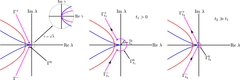
Figure 2: Left: Fredholm borders of $\mathcal{L}$ (blue, red) together with integration contour $\Gamma=\Gamma^{+}\cup\Gamma^{0}\cup\Gamma^{-}$ (magenta) used in the proof of Proposition 4.2. Center and right: integration contours (magenta) used in the proof of Proposition 4.4 at times $t_{1}$ (center) and $t_{2}>t_{1}$ (right).

The previous results trade spatial localization for temporal decay. The next result obtains decay of derivatives without loss of localization.

Proposition 4.4.

Let $r>2$. There exists a constant $C>0$ such that for any $z_{0}\in L^{\infty}_{r}(\mathbb{R})$, we have

$$\|\partial_{x}e^{\mathcal{L}t}z_{0}\|_{L^{\infty}_{r}}\leq\frac{C}{t^{3/2-r/2}}\|z_{0}\|_{L^{\infty}_{r}},$$ (4.6)

and

$$\|\partial_{x}e^{\mathcal{L}t}z_{0}\|_{L^{1}_{1}}\leq\frac{C}{t^{1/2}}\|z_{0}\|_{L^{\infty}_{r}}$$ (4.7)

for all $t>1$.

Proof.

We differentiate (4.2) and proceed as in [4, Proposition 7.4], choosing $\Gamma$ to be a circular arc centered at the origin whose radius scales as $t^{-1}$, connected to two rays extending out to infinity in the left half plane; see Figure 2. The estimates in Proposition 3.6 on the blowup of derivatives of the resolvent near the origin then translate into the claimed decay rates. ∎

Finally, we record useful small time regularity estimates for $e^{\mathcal{L}t}$.

Lemma 4.5.

There exists a constant $C>0$ such that

$$\|e^{\mathcal{L}t}z_{0}\|_{L^{\infty}}\leq\frac{C}{t^{1/2m}}\|z_{0}\|_{L^{1}}$$ (4.8)

for all $0<t<2$.

Proof.

Set $\mathcal{L}_{0}=(-1)^{m+1}\partial_{x}^{2m}$, and write $\mathcal{L}=\mathcal{L}_{0}+(\mathcal{L}-\mathcal{L}_{0})$. Using the Fourier transform yields

$$\|e^{\mathcal{L}_{0}t}z_{0}\|_{L^{\infty}}\leq\frac{C}{t^{1/2m}}\|z_{0}\|_{L^{1}}.$$ (4.9)

We then write $e^{\mathcal{L}t}z_{0}$ in mild form, viewing $\mathcal{L}$ as a perturbation of $\mathcal{L}_{0}$, so that

$$z(t):=e^{\mathcal{L}t}z_{0}=e^{\mathcal{L}_{0}t}z_{0}+\int_{0}^{t}e^{\mathcal{L}_{0}(t-s)}[(\mathcal{L}-\mathcal{L}_{0})z(s)]\,ds.$$ (4.10)

Since $(\mathcal{L}-\mathcal{L}_{0})$ is a differential operator of order $2m-1$ with smooth bounded coefficients, the Gagliardo-Nirenberg-Sobolev inequality allows us to control the integrand and obtain the desired estimate through a contraction argument in temporally weighted spaces. ∎

Similarly, we obtain the following small time bounds on derivatives of solutions.

Lemma 4.6.

Let $r>2$. There exists a constant $C>0$ such that

$$\|\partial_{x}e^{\mathcal{L}t}z_{0}\|_{L^{\infty}_{r}}\leq\frac{C}{t^{1/2m}}\|z_{0}\|_{L^{\infty}_{r}},$$ (4.11)

and

$$\|\partial_{x}e^{\mathcal{L}t}z_{0}\|_{L^{1}_{1}}\leq\frac{C}{t^{1/2m}}\|z_{0}\|_{L^{1}_{1}}$$ (4.12)

for all $0<t<2$.

5 Stability argument

Recall from Section 2.4 that our goal is to use the sharp linear estimates obtained in Section 4 to control perturbations to the approximate solution. We start by letting $v$ solve solve $\mathrm{F}_{\mathrm{res}}[v]=0$, where $\mathrm{F}_{\mathrm{res}}$ is given by (2.2), which is the original equation (1.6) in the co-moving frame with the logarithmic delay, and with the exponential weight $\omega$. We then define the perturbation $w=v-\psi$, which solves

$$w_{t}=\mathcal{L}w-f^{\prime}(q_{*})w-\frac{3}{2\eta_{*}(t+T)}\left[\omega(\omega^{-1})^{\prime}w+w_{x}\right]+\omega f(\omega^{-1}w+\psi)-\omega f(\omega^{-1}\psi)-R,$$ (5.1)

where $R=\mathrm{F}_{\mathrm{res}}[\psi]$. Note that $\omega^{-1}\psi$ is uniformly bounded, so by Taylor’s theorem,

$$\omega|N(\omega^{-1}w)|\leq C\omega^{-1}w^{2},$$ (5.2)

and

$$|(f^{\prime}(\omega^{-1}\psi)-f^{\prime}(q_{*}))w|\leq C|\omega^{-1}\psi-q_{*}||w|$$ (5.3)

for some constant $C>0$.

Recall that, in order to deal with the presence of the critical term $-\frac{3}{2\eta_{*}}(t+T)^{-1}\omega(\omega^{-1}w)$ in the $w$-equation, we introduce the new variable $z=(t+T)^{-3/2}w$, which solves

$$z_{t}=\mathcal{L}z-\frac{3}{2\eta_{*}(t+T)}[\omega(\omega^{-1})^{\prime}+\eta_{*}]z-\frac{3}{2\eta_{*}(t+T)}z_{x}+[f^{\prime}(\omega^{-1}\psi)-f^{\prime}(q_{*})]z-(t+T)^{-3/2}R\\ +(t+T)^{-3/2}\omega N(\omega^{-1}(t+T)^{3/2}z).$$ (5.4)

Note that $\omega(\omega^{-1})^{\prime}(x)+\eta_{*}\equiv 0$ for $x>1$, so that this term is essentially removed, which ultimately allows us to regain the $t^{-3/2}$ decay for $z$, equivalent to boundedness for $w$. This argument requires some care, however: we must track dependence on $T$, and compensate for the extra factor of $(t+T)^{3/2}$ now appearing with the nonlinearity. Tracking the $T$ dependence is necessary since we will treat linear terms such as $-\frac{3}{\eta_{*}}(t+T)^{-1}z_{x}$ perturbatively, and so we use largeness of $T$ to guarantee that these terms remain small, and because we need to track the $T$ dependence of $z$ in order to conclude that $w=(t+T)^{3/2}z$ is bounded. To handle the nonlinearity, note that, by Taylor’s theorem and exponential decay of $\omega^{-1}$, there exists a non-decreasing function $K:\mathbb{R}_{+}\to\mathbb{R}_{+}$ such that

$$\|(t+T)^{-3/2}\omega N(\omega^{-1}(t+T)^{3/2}z)\|_{L^{\infty}_{r}}\leq K(B)(t+T)^{3/2}\|z\|_{L^{\infty}_{-1}}^{2},$$ (5.5)

provided $(t+T)^{3/2}\|\omega^{-1}z\|_{L^{\infty}}\leq B$. In summary, the nonlinearity gains spatial localization but carries a factor of $(t+T)^{3/2}$.

We rewrite (5.4) in mild form via the variation of constants formula

$$z(t)=e^{\mathcal{L}t}z_{0}+\mathcal{I}_{1}(t)+\mathcal{I}_{2}(t)+\mathcal{I}_{3}(t)+\mathcal{I}_{R}(t)+\mathcal{I}_{N}(t),$$ (5.6)

where

$$\mathcal{I}_{1}(t) =-\frac{3}{2\eta_{*}}\int_{0}^{t}e^{\mathcal{L}(t-s)}\left[(\omega(\omega^{-1})^{\prime}+\eta_{*})\frac{z(s)}{s+T}\right]\,ds,$$ (5.7)

$$\mathcal{I}_{2}(t) =-\frac{3}{2\eta_{*}}\int_{0}^{t}e^{\mathcal{L}(t-s)}\frac{z_{x}(s)}{s+T}\,ds,$$ (5.8)

$$\mathcal{I}_{3}(t) =\int_{0}^{t}e^{\mathcal{L}(t-s)}\left[(f^{\prime}(\omega^{-1}\psi(s))-f^{\prime}(q_{*}))z(s)\right]\,ds,$$ (5.9)

$$\mathcal{I}_{R}(t) =-\int_{0}^{t}e^{\mathcal{L}(t-s)}(s+T)^{-3/2}R(s)\,ds,$$ (5.10)

$$\mathcal{I}_{N}(t) =\int_{0}^{t}e^{\mathcal{L}(t-s)}[(s+T)^{-3/2}\omega N(\omega^{-1}(s+T)^{3/2}z(s))]\,ds.$$ (5.11)

By standard parabolic regularity [64, 44], the equation for $z$ is locally well-posed in $L^{\infty}_{r}(\mathbb{R})$ for any $r\in\mathbb{R}$, in the sense that given any small initial data $z_{0}\in L^{\infty}_{r}(\mathbb{R})$, the variation of constants formula (5.6) defines a unique solution $z(t)$ for $t\in(0,t_{*})$ to (5.4) with

$$\lim_{t\to 0^{+}}(\mathcal{L}-\lambda)^{-1}z(t)=(\mathcal{L}-\lambda)^{-1}z_{0}\text{ in }L^{\infty}_{r}(\mathbb{R})$$ (5.12)

for any $\lambda$ in the resolvent set of $\mathcal{L}$. Furthermore, the maximal existence time $t_{*}$ depends only on $\|z_{0}\|_{L^{\infty}_{r}}$, and there is a constant $C>0$ such that for $t$ sufficiently small,

$$\|z_{x}(t)\|_{L^{\infty}_{r}}\leq\frac{C}{t^{1/2m}}\|z_{0}\|_{L^{\infty}_{r}}.$$ (5.13)

Theorem 5.1.

Let $0<\mu<\frac{1}{8}$ and $r=2+\mu$. Choose $\zeta(t+T)$ as in Proposition 2.5, and let $R(t;T)$ be the associated nonlinear residual defined in (2.38). Then define

$$R_{0}=\sup_{T\geq T_{*}}\sup_{s>0}\,(s+T)^{1/2-4\mu}\|R(s;T)\|_{L^{\infty}_{r}},$$ (5.14)

which is finite for some $T_{*}$ sufficiently large by Proposition 2.5. There exist positive constants $C$ and $\varepsilon$ such that if $z_{0}\in L^{\infty}_{r}(\mathbb{R})$ with

$$T^{3/2}\|z_{0}\|_{L^{\infty}_{r}}+T^{-1/2+4\mu}R_{0}<\varepsilon,$$ (5.15)

then the solution $z(t)$ to (5.4) with initial data $z_{0}$ exists globally in time in $L^{\infty}_{-1}(\mathbb{R})$ and satisfies

$$\|z(t)\|_{L^{\infty}_{-1}}\leq\frac{C}{(t+T)^{3/2}}\left(T^{3/2}\|z_{0}\|_{L^{\infty}_{r}}+T^{-1/2+4\mu}R_{0}\right)$$ (5.16)

for all $t>0$.

Note that $z_{0}=T^{-3/2}w_{0}$, where $w_{0}$ is the initial data for (2.52), such that (5.15) only enforces smallness of $\|w_{0}\|_{L^{\infty}_{r}}$, independent of $T$.

The remainder of this section is dedicated to proving Theorem 5.1 by estimating terms in the variation of constants formula. A first attempt would aim to control $(t+T)^{3/2}\|z(t)\|_{L^{\infty}_{-1}}$, but $z_{x}$ also enters via the term $\mathcal{I}_{2}(t)$. Handling this term requires the most care: in order to obtain $t^{-3/2}$ decay there, one needs $z_{x}(s)$ to decay in $L^{1}_{1}(\mathbb{R})$, a norm that enforces localization. To close the argument, we then use the weaker decay of $z_{x}(s)$ in $L^{\infty}_{r}(\mathbb{R})$ according to the linear estimates in Proposition 4.4. We capture this bootstrapping procedure, as well as the small-time regularity of the solution in the norm template

$$\Theta(t)=\sup_{0<s<t}\bigg{[}(s+T)^{3/2}\|z(s)\|_{L^{\infty}_{-1}}+1_{\{0<s<1\}}T^{3/2}s^{1/2m}\left(\|z_{x}(s)\|_{L^{1}_{1}}+\|z_{x}(s)\|_{L^{\infty}_{r}}\right)\\ +1_{\{s\geq 1\}}T^{1/2}\left((s+T)^{1/2}\|z_{x}(s)\|_{L^{1}_{1}}+(s+T)^{\beta}\|z_{x}(s)\|_{L^{\infty}_{r}}\right)\bigg{]},$$ (5.17)

where $\beta=\frac{3}{2}-\frac{r}{2}=\frac{1}{2}-\frac{\mu}{2}$. With the spatio-temporal decay, uniformly in $T$, encoded in $\Theta(t)$, we eventually obtain global-in-time control of $\Theta(t)$ from the following local-in-time estimates.

Proposition 5.2.

Let $r=2+\mu$ with $0<\mu<\frac{1}{8}$. There exist positive constants $C_{0},C_{1},$ and $C_{2}$ independent of $z_{0}\in L^{\infty}_{r}(\mathbb{R})$ such that

$$\Theta(t)\leq C_{0}\left(T^{3/2}\|z_{0}\|_{L^{\infty}_{r}}+T^{-1/2+4\mu}R_{0}\right)+\frac{C_{1}}{T^{1/2-4\mu}}\Theta(t)+C_{2}K(B\Theta(t))\Theta(t)^{2},$$ (5.18)

for all $t\in(0,t_{*})$, where $B=\|\rho_{1}\omega^{-1}\|_{L^{\infty}}$, with $K$ as in (5.5) and $\rho_{1}$ given by (1.19).

We break the proof of this proposition into several parts according to the the estimates on $z(t)$ versus $z_{x}(t)$, and to the different terms in the variation of constants formula (5.6). For the remainder of this section, we fix $0<\mu<\frac{1}{8}$, $z_{0}\in L^{\infty}_{r}(\mathbb{R})$, and $T$ large, and let $t_{*}$ be the maximal existence time of $z(t)$ in $L^{\infty}_{-1}(\mathbb{R})$. Unless otherwise noted, constants in this section are independent of $z_{0}\in L^{\infty}_{r}(\mathbb{R})$ and $T\geq T_{*}$.

5.1 Heuristics for $\Theta(t)$

For $x$ large, the equation for $w$ at least formally resembles the equation $\mathrm{F}_{\mathrm{res}}[v]=0$ considered in Section 2. Revisiting the scaling variables analysis therein (compare (2.27)), we expect $w$ to develop a diffusive tail as well, so that to leading order, at large $x$,

$$w(x,t)\sim c_{0}(x+a)e^{-(x+a)^{2}/[4(t+T)]}$$ (5.19)

for some constant $c_{0}$ depending on the initial data. Since $z(x,t)=(t+T)^{-3/2}w(x,t)$, this yields

$$z(x,t)\sim c_{0}\frac{x+a}{(t+T)^{3/2}}e^{-(x+a)^{2}/[4(t+T)]}$$ (5.20)

for $x$ large. We expect dynamics to be driven by this diffusive tail and infer the decay rates of $z(x,t)$ from this approximation. Indeed, we see decay in $L^{\infty}_{-1}(\mathbb{R}_{+})$ with rate $(t+T)^{-3/2}$ in the right hand side of (5.20), and decay of the derivative in $L^{1}_{1}(\mathbb{R})$ with rate $(t+T)^{-1/2}$, as captured in (5.17).

However, we have $\|z_{0}\|_{L^{\infty}_{r}}\lesssim T^{-3/2}$, for the initial data, which we wish to encode in the constant $c_{0}$. For small times, we expect to retain this $T^{-3/2}$ estimates at the price of some blowup in $t$ according to small-time regularity estimates in Section 4, which we capture in the terms in (5.17) involving $0<s<1$. We then track how this smallness of the initial data propagates to large times by incorporating $1_{s\geq 1}(s+T)^{1/2}T^{\tilde{\beta}}\|z_{x}(s)\|_{L^{1}_{1}}$ into the definition of $\Theta(t)$, leaving $\tilde{\beta}$ free at first. Throughout the course of the proof (see in particular Proposition 5.10), we find that $\tilde{\beta}=\frac{1}{2}$ is the optimal choice, and this control just suffices to close our argument.

At this point, we can also identify why we needed sharp $L^{1}$-$L^{\infty}$ estimates to replace the $L^{2}$-based linear estimates of [4]. In order to control $\mathcal{I}_{2}(t)$ and obtain $t^{-3/2}$ decay of $z(t)$, we need the integrand in (5.8) to be bounded by $(t-s)^{-3/2}(s+T)^{-3/2}$. In order to extract $(t-s)^{-3/2}$ decay from $e^{\mathcal{L}(t-s)}$, we have to control $z_{x}(s)$ in a space $X$ for which an estimate $\|e^{\mathcal{L}t}\|_{X\to L^{\infty}_{-1}}\leq Ct^{-3/2}$ holds. From Proposition 3.1, we see that the weakest such norm on the scale of algebraically weighted $L^{p}$ spaces is $L^{1}_{1}(\mathbb{R})$. We need this weakest norm, since we also have to extract decay from $z_{x}(s)$ to obtain the $(s+T)^{-3/2}$ estimate. Indeed, for $r>2$ we have by Proposition 4.4

$$\|\partial_{x}e^{\mathcal{L}t}\|_{L^{\infty}_{r}\to L^{\infty}_{r}}\leq\frac{C}{t^{3/2-r/2}},$$

a decay is strictly slower than $t^{-1/2}$, which would not enable us to obtain the necessary $(s+T)^{-3/2}$ decay in the integrand and close the argument. This obstruction remains if we replace $L^{\infty}_{r}(\mathbb{R}),r>2$, with the corresponding $L^{2}$-based localization, $L^{2}_{\tilde{r}}(\mathbb{R}),\tilde{r}>\frac{3}{2}$. Measuring the derivative instead in $L^{1}_{1}(\mathbb{R})$ gives the sharp $t^{-1/2}$ estimate which suffices to close the estimates on $z(t)$.

The proof now proceeds by estimating norms of $z$ and $z_{x}$ through the variation-of-constant formula invoking $\Theta$ to control the right-hand side.

5.2 Control of $z(t)$

We start with estimates on $z(t)$.

Proposition 5.3 (Estimates on $z(t)$).

There exist constants $C_{0},C_{1}$ and $C_{2}>0$ such that

$$(t+T)^{3/2}\|z(t)\|_{L^{\infty}_{-1}}\leq C_{0}\left(T^{3/2}\|z_{0}\|_{L^{\infty}_{r}}+T^{-1/2+4\mu}R_{0}\right)+\frac{C_{1}}{T^{1/2-4\mu}}\Theta(t)+C_{2}K(B\Theta(t))\Theta(t)^{2}$$ (5.21)

for all $t\in(0,t_{*})$.

In the following, we estimate each term in the variation of constants formula. We prepare the proof with several lemmas. Throughout, we repeatedly use the following elementary inequality.

Lemma 5.4.

Let $\alpha\geq\frac{3}{2}$. There exists a constant $C>0$ such that for all $t>0$,

$$(t+T)^{3/2}\int_{0}^{t}\frac{1}{(1+t-s)^{3/2}}\frac{1}{(s+T)^{\alpha}}\,ds\leq\frac{C}{T^{\alpha-3/2}}.$$ (5.22)

Proof.

We split the integral into two pieces,

$$(t+T)^{3/2}\int_{0}^{t}\frac{1}{(1+t-s)^{3/2}}\frac{1}{(s+T)^{\alpha}}\,ds=(t+T)^{3/2}\left(\int_{0}^{t/2}+\int_{t/2}^{t}\right)\frac{1}{(1+t-s)^{3/2}}\frac{1}{(s+T)^{\alpha}}\,ds$$

In the second integral, $s\geq t/2$, and so

$$(t+T)^{3/2}\int_{t/2}^{t}\frac{1}{(1+t-s)^{3/2}}\frac{1}{(s+T)^{\alpha}}\,ds \leq C\frac{(t+T)^{3/2}}{(t+T)^{\alpha}}\int_{t/2}^{t}\frac{1}{(1+t-s)^{3/2}}\,ds$$

$$=\frac{C}{(t+T)^{\alpha-3/2}}\int_{0}^{t/2}\frac{1}{(1+\tau)^{3/2}}\,d\tau$$

$$\leq\frac{C}{T^{\alpha-3/2}}$$

since $\tau\mapsto(1+\tau)^{-3/2}$ is integrable on $[0,\infty]$. In the first integral, on $[0,t/2]$, we use $t-s\geq t/2$,

$$(t+T)^{3/2}\int_{0}^{t/2}\frac{1}{(1+t-s)^{3/2}}\frac{1}{(s+T)^{\alpha}}\,ds \leq C\frac{(t+T)^{3/2}}{(1+t)^{3/2}}\int_{0}^{t/2}\frac{1}{(s+T)^{\alpha}}\,ds$$

$$=C\frac{(t+T)^{3/2}}{(1+t)^{3/2}}T^{-\alpha}\int_{0}^{t/2}\frac{1}{(1+\frac{s}{T})^{\alpha}}\,ds$$

$$=C\frac{(t+T)^{3/2}}{(1+t)^{3/2}}T^{-\alpha+1}\int_{0}^{t/(2T)}\frac{1}{(1+\tau)^{\alpha}}\,d\tau,$$

where we substituted $\tau=\frac{s}{T}$. By Taylor’s theorem, there exists $C>0$ such that for $t\leq T$, we have

$$\int_{0}^{t/(2T)}\frac{1}{(1+\tau)^{\alpha}}\,d\tau\leq C\frac{t}{T},$$

since the left-hand side is a smooth function that vanishes at $t=0$. Hence for $t\leq T$, we have

$$(t+T)^{3/2}\int_{0}^{t/2}\frac{1}{(1+t-s)^{3/2}}\frac{1}{(s+T)^{\alpha}}\,ds\leq C\frac{(t+T)^{3/2}}{(1+t)^{3/2}}T^{-\alpha}t\leq\frac{C}{T^{\alpha-3/2}}\frac{t}{(1+t)^{3/2}}\leq\frac{C}{T^{\alpha-3/2}}.$$

For $t\geq T$, we write

$$\left(\frac{t+T}{1+t}\right)^{3/2}=\left(1+\frac{T-1}{1+t}\right)^{3/2}\leq C,$$

and so in this case

$$(t+T)^{3/2}\int_{0}^{t/2}\frac{1}{(1+t-s)^{3/2}}\frac{1}{(s+T)^{\alpha}}\,ds \leq C\frac{(t+T)^{3/2}}{(1+t)^{3/2}}T^{-\alpha+1}\int_{0}^{t/(2T)}\frac{1}{(1+\tau)^{\alpha}}\,d\tau$$

$$\leq CT^{-\alpha+1}\int_{0}^{\infty}\frac{1}{(1+\tau)^{5/2}}\,d\tau$$

$$\leq CT^{-\alpha+1}$$

$$\leq\frac{C}{T^{\alpha-3/2}},$$

which completes the proof of the lemma. ∎

Lemma 5.5 (Estimates on $\mathcal{I}_{1}(t)$ and $\mathcal{I}_{3}(t)$).

There exists a constant $C>0$ such that

$$(t+T)^{3/2}\|\mathcal{I}_{1}(t)+\mathcal{I}_{3}(t)\|_{L^{\infty}_{-1}}\leq\frac{C}{T^{1/2-4\mu}}\Theta(t)$$ (5.23)

for all $t\in(0,t_{*})$.

Proof.

Using the linear decay from Corollary 4.3, we have

$$(t+T)^{3/2}\|\mathcal{I}_{1}(t)\|_{L^{\infty}_{-1}}\leq C(t+T)^{3/2}\int_{0}^{t}\frac{1}{(1+t-s)^{3/2}}\frac{1}{s+T}\|(\omega(\omega^{-1})^{\prime}+\eta_{*})z(s)\|_{L^{\infty}_{r}}\,ds.$$

Since $\omega(\omega^{-1})^{\prime}+\eta_{*}$ is identically zero on the right, we can absorb any algebraic weights into this factor, so that in particular

$$\|(\omega(\omega^{-1})^{\prime}+\eta_{*})z(s)\|_{L^{\infty}_{r}}\leq C\|z(s)\|_{L^{\infty}_{-1}}.$$

By the definition of $\Theta(t)$, we then have

$$\|z(s)\|_{L^{\infty}_{-1}}\leq(s+T)^{-3/2}\Theta(s)\leq(s+T)^{-3/2}\Theta(t)$$

for $0<s\leq t$, and so

$$(t+T)^{3/2}\|\mathcal{I}_{1}(t)\|_{L^{\infty}_{-1}} \leq C(t+T)^{3/2}\int_{0}^{t}\frac{1}{(1+t-s)^{3/2}}\frac{1}{s+T}\|z(s)\|_{L^{\infty}_{-1}}\,ds$$

$$\leq C\Theta(t)(t+T)^{3/2}\int_{0}^{t}\frac{1}{(1+t-s)^{3/2}}\frac{1}{(s+T)^{5/2}}\,ds.$$

By Lemma 5.4, we have

$$(t+T)^{3/2}\int_{0}^{t}\frac{1}{(1+t-s)^{3/2}}\frac{1}{(s+T)^{5/2}}\,ds\leq\frac{C}{T}$$

for all $t>0$, so that

$$(t+T)^{3/2}\|\mathcal{I}_{1}(t)\|_{L^{\infty}_{-1}}\leq\frac{C}{T}\Theta(t).$$

We next turn to $\mathcal{I}_{3}(t)$. With the linear decay estimate in Corollary 4.3 we have

$$(t+T)^{3/2}\|\mathcal{I}_{3}(t)\|_{L^{\infty}_{-1}} \leq C(t+T)^{3/2}\int_{0}^{t}\frac{1}{(1+t-s)^{3/2}}\|(f^{\prime}(\omega^{-1}\psi(s))-f^{\prime}(q_{*}))z(s)\|_{L^{\infty}_{r}}\,ds$$

$$\leq C(t+T)^{3/2}\int_{0}^{t}\frac{1}{(1+t-s)^{3/2}}\|f^{\prime}(\omega^{-1}\psi(s))-f^{\prime}(q_{*})\|_{L^{\infty}_{r+1}}\|z(s)\|_{L^{\infty}_{-1}}\,ds.$$

By Lemma 2.8 and the fact that $f$ is smooth,

$$\|f^{\prime}(\omega^{-1}\psi(s))-f^{\prime}(q_{*})\|_{L^{\infty}_{r+1}}\leq C\|\omega^{-1}\psi(s)-q_{*}\|_{L^{\infty}_{r+1}}\leq\frac{C}{(s+T)^{1/2-4\mu}},$$

so that

$$(t+T)^{3/2}\|\mathcal{I}_{3}(t)\|_{L^{\infty}_{-1}}\leq C(t+T)^{3/2}\Theta(t)\int_{0}^{t}\frac{1}{(1+t-s)^{3/2}}\frac{1}{(s+T)^{2-4\mu}}\,ds,$$

using also the definition of $\Theta(t)$ to extract a factor of $(s+T)^{-3/2}$ from $\|z(s)\|_{L^{\infty}_{-1}}$. By Lemma 5.4, we have

$$(t+T)^{3/2}\int_{0}^{t}\frac{1}{(1+t-s)^{3/2}}\frac{1}{(s+T)^{2-4\mu}}\,ds\leq\frac{C}{T^{1/2-4\mu}},$$

and hence

$$(t+T)^{3/2}\|\mathcal{I}_{3}(t)\|_{L^{\infty}_{-1}}\leq\frac{C}{T^{1/2-4\mu}}\Theta(t),$$

which completes the proof of the lemma. ∎

Lemma 5.6 (Estimates on $\mathcal{I}_{R}(t)$).

Let $r=2+\mu$. There exists a constant $C>0$ such that

$$(t+T)^{3/2}\|\mathcal{I}_{R}(t)\|_{L^{\infty}_{-1}}\leq\frac{C}{T^{1/2-4\mu}}R_{0}$$ (5.24)

for all $t\in(0,t_{*})$.

Proof.

Using linear decay from Corollary 4.3 and control of the residual from Proposition 2.5 yields

$$(t+T)^{3/2}\|\mathcal{I}_{R}(t)\|_{L^{\infty}_{-1}} \leq C(t+T)^{3/2}\int_{0}^{t}\frac{1}{(1+t-s)^{3/2}}\frac{1}{(s+T)^{3/2}}\|R(s;T)\|_{L^{\infty}_{r}}\,ds$$

$$\leq CR_{0}(t+T)^{3/2}\int_{0}^{t}\frac{1}{(1+t-s)^{3/2}}\frac{1}{(s+T)^{2-4\mu}}\,ds$$

$$\leq\frac{C}{T^{1/2-4\mu}}R_{0},$$

where the final estimate follows from Lemma 5.4. ∎

We next estimate the nonlinearity.

Lemma 5.7 (Estimates on $\mathcal{I}_{N}(t)$).

There exists a constant $C>0$ such that

$$(t+T)^{3/2}\|\mathcal{I}_{N}(t)\|_{L^{\infty}_{-1}}\leq CK(B\Theta(t))\Theta(t)^{2}$$ (5.25)

for all $t\in(0,t_{*})$.

Proof.

By the decay estimate in Corollary 4.3 together with the quadratic estimate (5.5) on the nonlinearity, we have

$$(t+T)^{3/2} \|\mathcal{I}_{N}(t)\|_{L^{\infty}_{-1}}$$

$$\leq C(t+T)^{3/2}\int_{0}^{t}\frac{1}{(1+t-s)^{3/2}}\|(s+T)^{-3/2}\omega N(\omega^{-1}(s+T)^{3/2}z(s))\|_{L^{\infty}_{r}}\,ds$$

$$\leq C(t+T)^{3/2}\int_{0}^{t}\frac{1}{(1+t-s)^{3/2}}K\left(\|\omega^{-1}(s+T)^{3/2}z(s)\|_{L^{\infty}}\right)(s+T)^{3/2}\|z(s)\|_{L^{\infty}_{-1}}^{2}\,ds$$

$$\leq C(t+T)^{3/2}\int_{0}^{t}\frac{1}{(1+t-s)^{3/2}}K(B\Theta(s))(s+T)^{3/2}\|z(s)\|_{L^{\infty}_{-1}}^{2}\,ds$$

$$\leq CK(B\Theta(t))\Theta(t)^{2}\int_{0}^{t}\frac{1}{(1+t-s)^{3/2}}\frac{1}{(s+T)^{3/2}}\,ds,$$

where we have also used that $K$ and $\Theta$ are non-decreasing. By Lemma 5.4, there exists a constant $C>0$ such that

$$\int_{0}^{t}\frac{1}{(1+t-s)^{3/2}}\frac{1}{(s+T)^{3/2}}\,ds\leq C.$$

Hence we obtain

$$(t+T)^{3/2}\|\mathcal{I}_{N}(t)\|_{L^{\infty}_{-1}}\leq CK(B\Theta(t))\Theta(t)^{2},$$

as desired. ∎

We finally estimate $\mathcal{I}_{2}(t)$, using the decay of $z_{x}(t)$ in $L^{1}_{1}(\mathbb{R})$ which we have encoded into the definition of $\Theta(t)$.

Lemma 5.8 (Estimates on $\mathcal{I}_{2}(t)$).

There exists a constant $C>0$ such that

$$(t+T)^{3/2}\|\mathcal{I}_{2}(t)\|_{L^{\infty}_{-1}}\leq\frac{C}{T^{1/2}}\Theta(t)$$ (5.26)

for all $t\in(0,t_{*})$.

Proof.

First assume $0<t<1$. Using the small time regularity estimate from Lemma 4.5, we have

$$(t+T)^{3/2}\|\mathcal{I}_{2}(t)\|_{L^{\infty}_{-1}} \leq C(t+T)^{3/2}\int_{0}^{t}\frac{1}{(t-s)^{1/2m}}\frac{1}{s+T}\|z_{x}(s)\|_{L^{1}_{1}}\,ds$$

$$\leq C(t+T)^{3/2}T^{-3/2}\Theta(t)\int_{0}^{t}\frac{1}{(t-s)^{1/2m}}\frac{1}{s+T}s^{-1/2m}\,ds,$$

where the last estimate follows from the definition (5.17) of $\Theta(t)$. Since for $t<1$, $(t+T)^{3/2}\leq CT^{3/2}$, we have

$$(t+T)^{3/2}\|\mathcal{I}_{2}(t)\|_{L^{\infty}_{-1}}\leq C\Theta(t)\int_{0}^{t}\frac{1}{(t-s)^{1/2m}}\frac{s^{-1/2m}}{s+T}\,ds \leq\frac{C}{T}\Theta(t)\int_{0}^{t}\frac{1}{(t-s)^{1/2m}}s^{-1/2m}\,ds\leq\frac{C}{T}\Theta(t).$$

Next, we consider $1\leq t<2$. Here we split the integral into two pieces, since the estimates on $z_{x}(s)$ encoded in the definition of $\Theta(t)$ differ for $s<1$ and $s>1$. We write

$$(t+T)^{3/2}\|\mathcal{I}_{2}(t)\|_{L^{\infty}_{-1}}\leq C(t+T)^{3/2}\left[\int_{0}^{1}\left\|e^{\mathcal{L}(t-s)}\frac{z_{x}(s)}{s+T}\right\|_{L^{\infty}_{-1}}\,ds+\int_{1}^{t}\left\|e^{\mathcal{L}(t-s)}\frac{z_{x}(s)}{s+T}\right\|_{L^{\infty}_{-1}}\,ds\right].$$

We estimate the first integral as in the $0<t<1$ case above and thereby obtain

$$(t+T)^{3/2}\int_{0}^{1}\left\|e^{\mathcal{L}(t-s)}\frac{z_{x}(s)}{s+T}\right\|_{L^{\infty}_{-1}}\leq\frac{C}{T}\Theta(t).$$

For the integral from $1$ to $t$, we again use Lemma 4.5 to estimate $\|e^{\mathcal{L}(t-s)}\|_{L^{1}_{1}\to L^{\infty}_{-1}}$, but the estimate on $\|z_{x}(s)\|_{L^{1}_{1}}$ differs slightly for $s>1$, so that we obtain

$$(t+T)^{3/2}\int_{1}^{t}\left\|e^{\mathcal{L}(t-s)}\frac{z_{x}(s)}{s+T}\right\|_{L^{\infty}_{-1}}\,ds \leq CT^{3/2}\int_{1}^{t}\frac{1}{(t-s)^{1/2m}}\frac{\|z_{x}(s)\|_{L^{1}_{1}}}{s+T}\,ds$$

$$\leq CT^{3/2}\Theta(t)\int_{1}^{t}\frac{1}{(t-s)^{1/2m}}\frac{1}{(s+T)^{3/2}}T^{-1/2}\,ds$$

$$\leq\frac{C}{T^{1/2}}\Theta(t)\int_{1}^{t}\frac{1}{(t-s)^{1/2m}}\,ds$$

$$\leq\frac{C}{T^{1/2}}\Theta(t).$$

It remains only to obtain the estimate for $t\geq 2$. For this, we split the integral into four pieces,

$$(t+T)^{3/2}\|\mathcal{I}_{2}(t)\|_{L^{\infty}_{-1}}\leq C(t+T)^{3/2}\bigg{[}\int_{0}^{1}+\int_{1}^{t/2}+\int_{t/2}^{t-1}+\int_{t-1}^{t}\bigg{]}\left\|e^{\mathcal{L}(t-s)}\frac{z_{x}(s)}{s+T}\right\|_{L^{\infty}_{-1}}\,ds.$$

We split the integral in this manner because we have to handle separately: the blowup of $z_{x}(s)$ when $s\sim 0$; the decay of $e^{\mathcal{L}(t-s)}$ when $(t-s)\sim t$; the decay of $z_{x}(s)$ when $s\sim t$; and the blowup of $e^{\mathcal{L}(t-s)}$ when $(t-s)\sim 0$.

For the first integral, we have $(t-s)\geq t/2\geq 1$, and by Proposition 4.2 and the definition of $\Theta(t)$,

$$(t+T)^{3/2}\int_{0}^{1}\left\|e^{\mathcal{L}(t-s)}\frac{z_{x}(s)}{s+T}\right\|_{L^{\infty}_{-1}}\,ds \leq C(t+T)^{3/2}\int_{0}^{1}\frac{1}{(t-s)^{3/2}}\frac{\|z_{x}(s)\|_{L^{1}_{1}}}{s+T}\,ds$$

$$\leq C\frac{(t+T)^{3/2}}{t^{3/2}}T^{-3/2}\Theta(t)\int_{0}^{1}\frac{s^{-1/2m}}{s+T}\,ds$$

$$\leq\frac{C}{T}\Theta(t)\int_{0}^{1}s^{-1/2m}\,ds$$

$$\leq\frac{C}{T}\Theta(t).$$

For the integral from $1$ to $t/2$, we still have $(t-s)\geq t/2\geq 1$, but the estimate on $z_{x}(s)$ differs, so that

$$(t+T)^{3/2}\int_{1}^{t/2}\left\|e^{\mathcal{L}(t-s)}\frac{z_{x}(s)}{s+T}\right\|_{L^{\infty}_{-1}}\,ds \leq C\frac{(t+T)^{3/2}}{t^{3/2}}\Theta(t)T^{-1/2}\int_{1}^{t/2}\frac{1}{(s+T)^{3/2}}\,ds.$$ (5.27)

For the remaining integral, arguing as in Lemma 5.4, we obtain

$$\frac{(t+T)^{3/2}}{t^{3/2}}T^{-1/2}\int_{1}^{t/2}\frac{1}{(s+T)^{3/2}}\,ds\leq\frac{C}{T^{1/2}},$$

so that

$$(t+T)^{3/2}\int_{1}^{t/2}\left\|e^{\mathcal{L}(t-s)}\frac{z_{x}(s)}{s+T}\right\|_{L^{\infty}_{-1}}\,ds\leq\frac{C}{T^{1/2}}\Theta(t).$$

For the integral from $t/2$ to $t-1$, we have $(t-s)\geq 1$ and $s\geq t/2$, so we use the linear decay from Proposition 4.2 to estimate

$$(t+T)^{3/2}\int_{t/2}^{t-1}\left\|e^{\mathcal{L}(t-s)}\frac{z_{x}(s)}{s+T}\right\|_{L^{\infty}_{-1}}\,ds \leq C(t+T)^{3/2}\int_{t/2}^{t-1}\frac{1}{(t-s)^{3/2}}\frac{\|z_{x}(s)\|_{L^{1}_{1}}}{s+T}\,ds$$

$$\leq C(t+T)^{3/2}\Theta(t)T^{-1/2}\int_{t/2}^{t-1}\frac{1}{(t-s)^{3/2}}\frac{1}{(s+T)^{3/2}}\,ds$$

$$\leq C\frac{(t+T)^{3/2}}{(t+T)^{3/2}}\Theta(t)T^{-1/2}\int_{t/2}^{t-1}\frac{1}{(t-s)^{3/2}}\,ds$$

$$=\frac{C}{T^{1/2}}\Theta(t)\int_{1}^{t/2}\frac{1}{\tau^{3/2}}\,d\tau$$

$$\leq\frac{C}{T^{1/2}}\Theta(t).$$

Finally, for the integral from $t-1$ to $t$, we use Lemma 4.5 to estimate

$$(t+T)^{3/2}\int_{t-1}^{t}\left\|e^{\mathcal{L}(t-s)}\frac{z_{x}(s)}{s+T}\right\|_{L^{\infty}_{-1}}\,ds \leq C(t+T)^{3/2}\int_{t-1}^{t}\frac{1}{(t-s)^{1/2m}}\frac{\|z_{x}(s)\|_{L^{1}_{1}}}{s+T}\,ds$$

$$\leq C(t+T)^{3/2}\Theta(t)T^{-1/2}\int_{t-1}^{t}\frac{1}{(t-s)^{1/2m}}\frac{1}{(s+T)^{3/2}}\,ds$$

$$\leq\frac{C}{T^{1/2}}\frac{(t+T)^{3/2}}{(t+T)^{3/2}}\Theta(t)\int_{t-1}^{t}\frac{1}{(t-s)^{1/2m}}\,ds$$

$$\leq\frac{C}{T^{1/2}}\Theta(t),$$

since $s\sim t$ in this region. This completes the proof of the lemma. ∎

We emphasize that the proof of Lemma 5.8 shows that control of $z(t)$ necessitates good estimates on $\|z_{x}(t)\|_{L^{1}_{1}}$. We now gather the individual estimates on terms in $z(t)$ for the proof of Proposition 5.3, and thereby establish control of $\|z(t)\|_{L^{\infty}_{-1}}$ provided appropriate control of $z_{x}(t)$.

Proof of Proposition 5.3.

With Lemmas 5.5 through 5.8 at hand, it only remains to estimate the term in the variation of constants formula (5.6) involving the initial data, for which we have, by the linear decay estimate in Corollary 4.3,

$$(t+T)^{3/2}\|e^{\mathcal{L}t}z_{0}\|_{L^{\infty}_{-1}}\leq C\frac{(t+T)^{3/2}}{(1+t)^{3/2}}\|z_{0}\|_{L^{\infty}_{r}}\leq CT^{3/2}\|z_{0}\|_{L^{\infty}_{r}},$$

which completes the proof of the proposition. ∎

5.3 Control of derivatives

To complete the proof of Proposition 5.2, we now estimate $z_{x}(t)$. We therefore differentiate the variation of constants formula, obtaining

$$z_{x}(t)=\partial_{x}(e^{\mathcal{L}t}z_{0})+\partial_{x}\mathcal{I}_{1}(t)+\partial_{x}\mathcal{I}_{2}(t)+\partial_{x}\mathcal{I}_{3}(t)+\partial_{x}\mathcal{I}_{R}(t)+\partial_{x}\mathcal{I}_{N}(t).$$ (5.28)

We need estimates on $\|z_{x}(t)\|_{L^{1}_{1}}$ to close the argument for $\|z(t)\|_{L^{\infty}_{-1}}$, and in turn we need estimates on $\|z_{x}(t)\|_{L^{\infty}_{r}}$ to close the argument for $\|z_{x}(t)\|_{L^{1}_{1}}$. We thereby rely on the sharp linear estimates on derivatives from Section 4.

Proposition 5.9 (Small time estimates on $z_{x}(t)$).

Let $r=2+\mu$ with $0<\mu<\frac{1}{8}$. There exist constants $C_{0},C_{1},$ and $C_{2}>0$ such that

$$T^{3/2}t^{1/2m}\|z_{x}(t)\|_{X}\leq C_{0}\left(T^{3/2}\|z_{0}\|_{L^{\infty}_{r}}+T^{-1/2+4\mu}R_{0}\right)+\frac{C_{1}}{T^{1/2-4\mu}}\Theta(t)+C_{2}K(B\Theta(t))\Theta(t)^{2}$$ (5.29)

for all $0\leq t<\min(1,t_{*})$, where $X=L^{1}_{1}(\mathbb{R})$ or $L^{\infty}_{r}(\mathbb{R})$.

Proof.

For the term involving the initial data in (5.28), we have by Lemma 4.6,

$$T^{3/2}t^{1/2m}\|\partial_{x}(e^{\mathcal{L}t}z_{0})\|_{X}\leq CT^{3/2}\|z_{0}\|_{L^{1}_{1}}\leq CT^{3/2}\|z_{0}\|_{L^{\infty}_{r}}.$$

We now focus on the term involving $\mathcal{I}_{N}(t)$, as this term is the closest to critical, in the sense that if its $T$ dependence were any worse, we would not be able to close the argument. By Lemma 4.6 and the estimate (5.5) on the nonlinearity, we have

$$T^{3/2}t^{1/2m}\|\partial_{x}\mathcal{I}_{N}(t)\|_{X} \leq CT^{3/2}t^{1/2m}\int_{0}^{t}\frac{1}{(t-s)^{1/2m}}\|(s+T)^{-3/2}\omega N(\omega^{-1}(s+T)^{3/2}z(s))\|_{L^{\infty}_{r}}\,ds$$

$$\leq CK(B\Theta(t))T^{3/2}t^{1/2m}\int_{0}^{t}\frac{1}{(t-s)^{1/2m}}(s+T)^{3/2}\|z(s)\|_{L^{\infty}_{-1}}^{2}\,ds$$

$$\leq CK(B\Theta(t))\Theta(t)^{2}T^{3/2}t^{1/2m}\int_{0}^{t}\frac{1}{(t-s)^{1/2m}}\frac{1}{(s+T)^{3/2}}\,ds$$

$$\leq CK(B\Theta(t))\Theta(t)^{2}t^{1/2m}\int_{0}^{t}\frac{1}{(t-s)^{1/2m}}\,ds$$

$$\leq CK(B\Theta(t))\Theta(t)^{2}$$

for $0<t<1$, as desired. We readily obtain the estimates on the other terms by similar arguments. ∎

Proposition 5.10 (Large time $L^{1}_{1}$ estimates on $z_{x}(t)$).

There exist constants $C_{0},C_{1}$, and $C_{2}>0$ such that for all $t\in[1,t_{*})$,

$$(t+T)^{1/2}T^{1/2}\|z_{x}(t)\|_{L^{1}_{1}}\leq C_{0}\left(T^{3/2}\|z_{0}\|_{L^{\infty}_{r}}+T^{-1/2+4\mu}R_{0}\right)+\frac{C_{1}}{T^{1/2-4\mu}}\Theta(t)+C_{2}K(B\Theta(t))\Theta(t)^{2}.$$ (5.30)

Proof.

The two most important terms in (5.28) are $\partial_{x}\mathcal{I}_{N}(t)$ and $\partial_{x}\mathcal{I}_{2}(t)$. The first one is the closest to critical and thereby determines the optimal choice of $\tilde{\beta}$ in the definition of $\Theta(t)$ as discussed in Section 5.1. The estimates on the term $\partial_{x}\mathcal{I}_{2}(t)$ reveal how we can close our bootstrapping argument by relying on the lack of criticality in this term.

We focus first on $\partial_{x}\mathcal{I}_{N}(t)$, for which we have

$$(t+T)^{1/2}T^{1/2}\|\partial_{x}\mathcal{I}_{N}(t)\|_{L^{1}_{1}}\leq C(t+T)^{1/2}T^{1/2}\int_{0}^{t}\left\|\partial_{x}e^{\mathcal{L}(t-s)}\tilde{N}(z(s),s;T)\right\|_{L^{1}_{1}}\,ds,$$

where

$$\tilde{N}(z(s),s;T)=(s+t)^{-3/2}\omega N(\omega^{-1}(s+T)^{3/2}z(s)).$$ (5.31)

We split the integral into an integral from $0$ to $t/2$ and another from $t/2$ to $t$. For the integral from $0$ to $t/2$, we use Proposition 4.4 together with the estimate (5.5) to obtain

$$\int_{0}^{t/2}\left\|\partial_{x}e^{\mathcal{L}(t-s)}\tilde{N}(z(s),s;T)\right\|_{L^{1}_{1}}\,ds\leq CK(B\Theta(t))\Theta(t)^{2}\int_{0}^{t/2}\frac{1}{(t-s)^{1/2}}\frac{1}{(s+T)^{3/2}}\,ds.$$ (5.32)

Inside the integral, $t-s\sim t$, so that

$$(t+T)^{1/2}T^{1/2}\int_{0}^{t/2}\frac{1}{(t-s)^{1/2}}\frac{1}{(s+T)^{3/2}}\,ds \leq Ct^{-1/2}(t+T)^{1/2}T^{1/2}\int_{0}^{t/2}\frac{1}{(s+T)^{3/2}}\,ds$$

$$=C\left(1+\frac{T}{t}\right)^{1/2}\int_{0}^{t/2T}\frac{1}{(1+\tau)^{3/2}}\,d\tau$$

$$\leq C.$$

Notably, we only get a constant bound here: there is no extra $T$ decay to extract, and so this estimate determines our choice for the form of $\Theta(t)$. Hence

$$(t+T)^{1/2}T^{1/2}\int_{0}^{t/2}\left\|\partial_{x}e^{\mathcal{L}(t-s)}\tilde{N}(z(s),s;T)\right\|_{L^{1}_{1}}\,ds\leq CK(B\Theta(t))\Theta(t)^{2}.$$

For the integral from $t/2$ to $t$, we have by Proposition 4.4, Lemma 4.6, and the estimate (5.5) on the nonlinearity,

$$\int_{t/2}^{t}\left\|\partial_{x}e^{\mathcal{L}(t-s)}\tilde{N}(z(s),s;T)\right\|_{L^{1}_{1}}\,ds\leq CK(B\Theta(t))\Theta(t)^{2}\int_{t/2}^{t}\frac{1}{(t-s)^{1/2}}\frac{1}{(s+T)^{3/2}}\,ds.$$

For the remaining integral, we have the elementary estimate

$$(t+T)^{1/2}T^{1/2}\int_{t/2}^{t}\frac{1}{(t-s)^{1/2}}\frac{1}{(s+T)^{3/2}}\,ds\leq\frac{C}{t+T}T^{1/2}t^{1/2}\leq C,$$

so that

$$(t+T)^{1/2}T^{1/2}\int_{t/2}^{t}\left\|\partial_{x}e^{\mathcal{L}(t-s)}\tilde{N}(z(s),s;T)\right\|_{L^{1}_{1}}\,ds\leq CK(B\Theta(t))\Theta(t)^{2}$$

as well, which completes the estimates for $\partial_{x}\mathcal{I}_{N}(t)$.

For the term involving $\partial_{x}\mathcal{I}_{2}(t)$, we focus on only the integral from $0$ to $t/2$, since the modifications to handle the other integral are similar to the above. For this term, we have by Proposition 4.4

$$(t+T)^{1/2}T^{1/2}\int_{0}^{t/2}\left\|\partial_{x}e^{\mathcal{L}(t-s)}\frac{z_{x}(s)}{s+T}\right\|_{L^{1}_{1}}\,ds\leq C(t+T)^{1/2}T^{1/2}\int_{0}^{t/2}\frac{1}{(t-s)^{1/2}}\frac{\|z_{x}(s)\|_{L^{\infty}_{r}}}{s+T}\,ds.$$

We then use the weaker decay of $\|z_{x}(s)\|_{L^{\infty}_{r}}$ built into $\Theta(t)$ to estimate

$$(t+T)^{1/2}T^{1/2}\int_{0}^{t/2}\frac{1}{(t-s)^{1/2}}\frac{\|z_{x}(s)\|_{L^{\infty}_{r}}}{s+T}\,ds\leq C\Theta(t)(t+T)^{1/2}\int_{0}^{t/2}\frac{1}{(t-s)^{1/2}}\frac{1}{(s+T)^{1+\beta}}\,ds.$$

Note that we have also absorbed the factor of $T^{1/2}$ with $\|z_{x}(s)\|_{L^{\infty}_{r}}$, using the construction of $\Theta(t)$. For the remaining integral, we have the elementary estimate

$$(t+T)^{1/2}\int_{0}^{t/2}\frac{1}{(t-s)^{1/2}}\frac{1}{(s+T)^{1+\beta}}\,ds \leq\frac{C}{t^{1/2}}(t+T)^{1/2}\int_{0}^{t/2}\frac{1}{(s+T)^{1+\beta}}\,ds$$

$$=CT^{-\beta}\left(1+\frac{T}{t}\right)^{1/2}\int_{0}^{t/2T}\frac{1}{(1+\tau)^{1+\beta}}\,d\tau$$

$$\leq CT^{-\beta}=\frac{C}{T^{1/2-\mu/2}}\leq\frac{C}{T^{1/2-4\mu}},$$

recalling that $\beta=\frac{1}{2}-\frac{\mu}{2}$. Estimating also the integral from $t/2$ to $t$ with similar arguments to the above, we obtain

$$(t+T)^{1/2}T^{1/2}\|\partial_{x}\mathcal{I}_{2}(t)\|_{L^{1}_{1}}\leq\frac{C}{T^{1/2-4\mu}}\Theta(t),$$

as desired. The estimates on $\partial_{x}\mathcal{I}_{1}(t),\partial_{x}\mathcal{I}_{3}(t),\partial_{x}\mathcal{I}_{R}(t)$, and $\partial_{x}(e^{\mathcal{L}t}z_{0})$ are similar. ∎

Proposition 5.11 (Large time $L^{\infty}_{r}$ estimates on $z_{x}(t)$).

Let $r=2+\mu$ with $0<\mu<\frac{1}{8}$. There exist constants $C_{0},C_{1}$, and $C_{2}>0$ such that

$$(t+T)^{\beta}T^{1/2}\|z_{x}(t)\|_{L^{\infty}_{r}}\leq C_{0}\left(T^{3/2}\|z_{0}\|_{L^{\infty}_{r}}+T^{-1/2+4\mu}R_{0}\right)+\frac{C_{1}}{T^{1/2-4\mu}}\Theta(t)+C_{2}K(B\Theta(t))\Theta(t)^{2}$$ (5.33)

for all $t\in[1,t_{*})$, where $\beta=\frac{3}{2}-\frac{r}{2}=\frac{1}{2}-\frac{\mu}{2}$.

Proof.

Since the proof is similar to that of Proposition 5.10, we only point out the crucial feature that allows us to terminate the bootstrapping procedure. By Proposition 4.4, we have

$$(t+T)^{\beta}T^{1/2}\|\partial_{x}\mathcal{I}_{2}(t)\|_{L^{\infty}_{r}}\leq C(t+T)^{\beta}T^{1/2}\int_{0}^{t}\frac{1}{(t-s)^{\beta}}\frac{\|z_{x}(s)\|_{L^{\infty}_{r}}}{s+T}\,ds.$$

Owing to the extra factor of $(s+T)^{-1}$ in the integrand, we can carry out exactly the same argument used to estimate $\|\partial_{x}\mathcal{I}_{2}(t)\|_{L^{1}_{1}}$ in the previous proposition here, and thereby obtain

$$(t+T)^{\beta}T^{1/2}\|\partial_{x}\mathcal{I}_{2}(t)\|_{L^{\infty}_{r}}\leq\frac{C}{T^{1/2-4\mu}}\Theta(t).$$

∎

5.4 Proof of Theorem 5.1

The full control of $\Theta(t)$, Proposition 5.2, follows directly from the control of $z(t)$ and $z_{x}(t)$ in Propositions 5.3, 5.9, 5.10, and 5.11.

Proof of Theorem 5.1.

By Proposition 5.2, for $T$ sufficiently large (so that $C_{1}/T^{1/2-4\mu}<1$) there exist constants $\tilde{C}_{0}$ and $\tilde{C}_{2}$ so that

$$\Theta(t)\leq\tilde{C}_{0}(T^{3/2}\|z_{0}\|_{L^{\infty}_{r}}+T^{-1/2+4\mu}R_{0})+\tilde{C}_{2}K(B\Theta(t))\Theta(t)^{2}.$$ (5.34)

From the local well-posedness theory, it follows that there exists a constant $C>0$ such that

$$\Theta(t)\leq CT^{3/2}\|z_{0}\|_{L^{\infty}_{r}}$$ (5.35)

for small times provided the initial data is sufficiently small. Suppose $\Omega_{0}:=T^{3/2}\|z_{0}\|_{L^{\infty}_{r}}+T^{-1/2+4\mu}R_{0}$ is small enough so that

$$2C_{0}\Omega_{0}<1\quad\text{ and }\quad 4C_{0}C_{2}K(B)\Omega_{0}<1.$$ (5.36)

We show that

$$\Theta(t)\leq 2C_{0}\Omega_{0}<1$$ (5.37)

for all $t\in(0,t_{*})$. By (5.35), $\Theta(t)\leq\Omega_{0}\leq 2C_{0}\Omega_{0}<1$ for $t$ sufficiently small (redefining $C_{0}$ so that $C_{0}>\frac{1}{2}$ if necessary). By construction, $t\mapsto\Theta(t)$ is continuous on $(0,t_{*})$. Hence if (5.37) does not hold, then there must be some time $t_{1}>0$ at which $\Theta(t_{1})=2C_{0}\Omega_{0}$. Considering (5.34) at time $t_{1}$, we obtain

$$2C_{0}\Omega_{0}\leq C_{0}\Omega_{0}+4K(B2C_{0}\Omega_{0})C_{0}^{2}C_{2}\Omega_{0}^{2}\leq C_{0}\Omega_{0}(1+4C_{0}C_{2}K(B)\Omega_{0})$$

since $K$ is non-decreasing and $2C_{0}\Omega_{0}<1$. Since also $4C_{0}C_{2}K(B)\Omega_{0}<1$, we conclude

$$2<1+4C_{0}C_{2}K(B)\Omega_{0}<2,$$

a contradiction. Therefore, $\Theta(t)\leq 2C_{0}\Omega_{0}$ for all $t\in(0,t_{*})$, which implies that $t_{*}=\infty$ by the local well-posedness theory. This global control on $\Theta(t)$ implies in particular

$$\|z(t)\|_{L^{\infty}_{-1}}\leq\frac{C}{(t+T)^{3/2}}\Omega_{0},$$

for some constant $C>0$, as desired. ∎

6 Consequences for front propagation — proof of Theorem 1

Let $u$ solve the original equation

$$u_{t}=\mathcal{P}(\partial_{y})u+f(u)$$ (6.1)

with initial data $u_{0}$. Here we use $y$ for the original stationary variable, since we will consider both the stationary and moving frames in this section. Indeed, we let

$$x=y-c_{*}t+\frac{3}{2\eta_{*}}\log(t+T)-\frac{3}{2\eta_{*}}\log(T),$$ (6.2)

and define $U(x,t)=u(y,t)$, so that $U$ solves the equation in the moving frame with initial data $U_{0}(x):=U(x,0)=u_{0}(x)$. We then let $v=\omega U$, so that $v$ solves $\mathrm{F}_{\mathrm{res}}[v]=0$, and let $w(x,t)=v(x,t)-\psi(x,t;T)$ be a perturbation to $\psi$, so that $w$ solves (2.52). The decay of $z(x,t)$ in Theorem 5.1 translates into the following stability result for $w$.

Corollary 6.1.

Let $r=2+\mu$ with $0<\mu<\frac{1}{8}$, and let $R_{0}$ be given by (5.14). There exist positive constants $C$ and $\varepsilon$ such that if $w_{0}\in L^{\infty}_{r}(\mathbb{R})$ with

$$\|w_{0}\|_{L^{\infty}_{r}}+T^{-1/2+4\mu}R_{0}<\varepsilon,$$ (6.3)

then the solution $w(x,t)$ exists for all positive time, and

$$\|w(\cdot,t)\|_{L^{\infty}_{-1}}\leq C\left(\|w_{0}\|_{L^{\infty}_{r}}+T^{-1/2+4\mu}R_{0}\right)$$ (6.4)

for all $t>0$.

Proof.

With $z(x,t)=(t+T)^{-3/2}w(x,t)$, smallness of $w_{0}$ implies smallness of $T^{3/2}z_{0}$, so that the assumptions of Theorem 5.1 are satisfied, and hence

$$\|w(\cdot,t)\|_{L^{\infty}_{-1}}=(t+T)^{3/2}\|z(\cdot,t)\|_{L^{\infty}_{-1}}\leq C\left(\|w_{0}\|_{L^{\infty}_{r}}+T^{-1/2+4\mu}R_{0}\right),$$

as desired. ∎

In other words, provided the initial data is close to $\psi(\cdot,0;T)$, the solution $U$ in the co-moving frame with the logarithmic shift is well-approximated by $\psi(\cdot,t;T)$ for all times.

Corollary 6.2.

Let $r=2+\mu$ with $0<\mu<\frac{1}{8}$. There exist positive constants $C$ and $\varepsilon$ such that if $U_{0}$ satisfies

$$\|\omega U_{0}-\psi(\cdot,0;T)\|_{L^{\infty}_{r}}+T^{-1/2+4\mu}R_{0}<\varepsilon,$$ (6.5)

then

$$\|\omega U(\cdot,t)-\psi(\cdot,t;T)\|_{L^{\infty}_{-1}}\leq C\left(\|\omega U_{0}-\psi(\cdot,0;T)\|_{L^{\infty}_{r}}+T^{-1/2+4\mu}R_{0}\right)$$ (6.6)

for all $t>0$.

Proof of Theorem 1.

Given $\varepsilon>0$ small enough so that Corollary 6.2 holds with this choice of $\varepsilon$, fix $T$ large enough so that $T^{-1/2+4\mu}R_{0}<\frac{\varepsilon}{4}$. We then define

$$\mathcal{U}_{\varepsilon}=\left\{U_{0}:\omega U_{0}\in L^{\infty}_{r}(\mathbb{R})\text{ and }\|\omega U_{0}-\psi(\cdot,0;T)\|_{L^{\infty}_{r}}+T^{-1/2+4\mu}R_{0}<\frac{\varepsilon}{2}\right\}.$$ (6.7)

For any fixed $T$, $\mathcal{U}_{\varepsilon}$ is clearly open in the norm $\|U_{0}\|_{\rho}=\|\rho_{r}\omega U_{0}\|_{L^{\infty}}$. If we define

$$\tilde{U}_{0}(x)=\begin{cases}\omega^{-1}(x)\psi(x,0;T),&x<T^{1/2+\mu}-x_{0},\\ 0,&x\geq T^{1/2+\mu}-x_{0},\end{cases}$$ (6.8)

then from the expression (2.27) for $\psi^{+}$, one sees that

$$\|\omega\tilde{U}_{0}-\psi(\cdot,0;T)\|_{L^{\infty}_{r}}\leq CT^{5/2+2\mu}\exp(-cT^{2\mu})$$ (6.9)

for some constants $C,c>0$. In particular, for $T$ sufficiently large depending on $\varepsilon$, we have $\tilde{U}_{0}\in\mathcal{U}_{\varepsilon}$, so that Definition 1, (ii), is satisfied by $\mathcal{U}_{\varepsilon}$. Recalling that $u(x+\tilde{\sigma}_{T}(t),t)=U(x,t)$ with

$$\tilde{\sigma}_{T}(t)=c_{*}t-\frac{3}{2\eta_{*}}\log(t+T)+\frac{3}{2\eta_{*}}\log(T),$$ (6.10)

we conclude from Corollary 6.2 that

$$\sup_{x\in\mathbb{R}}|\rho_{-1}(x)\omega(x)[u(x+\tilde{\sigma}_{T}(t),t)-\omega(x)^{-1}\psi(x,t;T)]|<\frac{\varepsilon}{2}.$$ (6.11)

for all $u_{0}\in\mathcal{U}_{\varepsilon}$. By Lemma 2.8, $\omega^{-1}\psi$ is a good approximation to the critical front, so that by the triangle inequality

$$\sup_{x\in\mathbb{R}}|\rho_{-1}(x)\omega(x)[u(x+\tilde{\sigma}_{T}(t),t)-q_{*}(x)]|<\frac{3\varepsilon}{4}$$ (6.12)

provided $T$ is sufficiently large. Then, if we define

$$\sigma(t)=c_{*}t-\frac{3}{2\eta_{*}}\log(t)-\frac{3}{2\eta_{*}}\log\left(\frac{1}{T}\right),$$ (6.13)

we see that for $T$ fixed

$$|\tilde{\sigma}_{T}(t)-\sigma(t)|=\left|\log\left(\frac{1}{1+t/T}\right)\right|\to 0\text{ as }t\to\infty.$$ (6.14)

Hence, since $u$ is smooth by parabolic regularity, for $t$ sufficiently large we can replace $\tilde{\sigma}_{T}(t)$ by $\sigma(t)$ in (6.12) to obtain

$$\sup_{x\in\mathbb{R}}|\rho_{-1}(x)\omega(x)[u(x+\sigma(t),t)-q_{*}(x)]|<\varepsilon$$ (6.15)

for $t$ sufficiently large, depending on $u_{0}$ via $T$. This is the refined estimate of Theorem 1, with

$$x_{\infty}(u_{0})=-\frac{3}{2\eta_{*}}\log\left(\frac{1}{T}\right).$$ (6.16)

In particular, $q_{*}$ is a selected front.

∎

7 Robustness of assumptions — proof of Theorem 2

We now consider an equation

$$u_{t}=\mathcal{P}(\partial_{x};\delta)u+f(u;\delta)$$ (7.1)

where $\mathcal{P}(\partial_{x};\delta)$ is an elliptic operator of order $2m$ whose coefficients are smooth in $\delta$, and where $f$ is smooth in both its arguments, with $f(0;\delta)=f(1;\delta)=0$ for $\delta$ small and $f^{\prime}(0;\delta)>0,f^{\prime}(1;\delta)<0$ for $\delta$ small. We assume that at $\delta=0$, Hypotheses 1 through 4 are satisfied, and we conclude here that these assumptions hold for $\delta$ small. Our argument is essentially that of [3] adapted to a general setting, without the additional technical difficulty of regularizing the singular perturbation.

We write the asymptotic dispersion relation on the right as

$$d(\lambda,\nu;c,\delta)=\mathcal{P}(\nu;\delta)+c\nu+f^{\prime}(0;\delta)-\lambda.$$ (7.2)

Since by assumption Hypothesis 1 holds at $\delta=0$, we have

$$d(0,-\eta_{0};c_{0},0)=\partial_{\nu}d(0,-\eta_{0};c_{0},0)=0$$ (7.3)

for some $c_{0},\eta_{0}>0$, and there is $\alpha_{0}>0$ such that

$$d(\lambda,\nu-\eta_{0};c_{0},0)=\alpha_{0}\nu^{2}-\lambda+\mathrm{O}(\nu^{3}).$$ (7.4)

Lemma 7.1 (Robustness of simple pinched double roots).

There exists $\delta_{0}>0$ and smooth functions $\eta_{*}:(-\delta_{0},\delta_{0})\to\mathbb{C}$ and $c_{*}:(-\delta_{0},\delta_{0})\to\mathbb{R}$ such that $\eta_{*}(0)=\eta_{0},c_{*}(0)=c_{0}$, and

$$d(0,-\eta_{*}(\delta);c_{*}(\delta),0)=\partial_{\nu}d(0,-\eta_{*}(\delta);c_{*}(\delta),0)=0$$ (7.5)

for all $\delta\in(-\delta_{0},\delta_{0})$. Furthermore, there is a smooth function $\alpha:(-\delta_{0},\delta_{0})\to\mathbb{R}_{+}$ such that $\alpha(0)=\alpha_{0}$ and for $\lambda$ and $\nu$ small, we have

$$d(\lambda,\nu-\eta_{*}(\delta);c_{*}(\delta),\delta)=\alpha(\delta)\nu^{2}-\lambda+\mathrm{O}(\nu^{3}),$$ (7.6)

where the $\mathrm{O}(\nu^{3})$ terms depend on $\delta$ as well. As a result, there are two roots $\nu^{\pm}$ of the dispersion relation $\nu\mapsto d(\gamma^{2},\nu-\eta_{*}(\delta);c_{*}(\delta),\delta)$ which satisfy

$$\nu^{\pm}(\gamma;\delta)=\pm\nu_{0}(\delta)\gamma+\mathrm{O}(\gamma^{2}),$$

for $\gamma$ small $\mathcal{L}(\delta)$, where $\nu_{0}(\delta)>0$ for $\delta$ small.

Proof.

Define $F:\mathbb{C}\times\mathbb{R}^{2}\to\mathbb{C}^{2}$ by

$$F(\nu,c;\delta)=\begin{pmatrix}d(0,\nu;c,\delta)\\ \partial_{\nu}d(0,\nu;c,\delta)\end{pmatrix}.$$ (7.7)

The result (7.5) is equivalent to $F(-\eta_{*}(\delta),c_{*}(\delta);\delta)=0$, and by assumption, we have $F(-\eta_{0},c_{0};0)=0$. The derivative of $F$ with respect to its first two arguments,

$$D_{\nu,c}F(-\eta_{0},c_{0};0)=\begin{pmatrix}0&-\eta_{0}\\ 2\alpha_{0}&0\end{pmatrix},$$ (7.8)

is invertible. Therefore, by the implicit function theorem, for $\delta$ small there exist $\eta_{*}(\delta)$ and $c_{*}(\delta)$ smooth in $\delta$ so that $F(-\eta_{*}(\delta),c_{*}(\delta);\delta)=0$, as desired. The expansion (7.6) follows from this smoothness and the smoothness of the original dispersion relation. For more details on continuity of linear spreading speeds, see [49]. ∎

We note that this lemma together with standard spectral perturbation theory implies that the essential spectrum of $\mathcal{L}(\delta)$ is marginally stable, touching the imaginary axis only at the origin, i.e. Hypothesis 1 is satisfied.

We now turn to the existence of the critical front. Let $q_{0}$ denote the critical front at $\delta=0$ and $\mathcal{L}(0)$ the linearization about that front, in the weighted space with weight $\omega_{0}$, where

$$\omega_{\delta}(x)=\begin{cases}e^{\eta_{*}(\delta)x},&x\geq 1,\\ 1,&x\leq-1.\end{cases}$$ (7.9)

Recall from Section 3 that our assumptions imply that $\mathcal{L}(0)$ is Fredholm with index -1 when considered as an operator from $H^{2m}_{\mathrm{exp},\eta}(\mathbb{R})\to L^{2}_{\mathrm{exp},\eta}(\mathbb{R})$ for $\eta>0$ small. By Hypothesis 4, the kernel of $\mathcal{L}(0)$ is trivial on this space, so it has a one-dimensional cokernel.

Lemma 7.2.

Let $\mathcal{L}(0)^{*}:H^{2m}_{\mathrm{exp},-\eta}(\mathbb{R})\subset L^{2}_{\mathrm{exp},-\eta}(\mathbb{R})\to L^{2}_{\mathrm{exp},-\eta}(\mathbb{R})$ be the $L^{2}$-adjoint of $\mathcal{L}(0)$, and let $\ker\mathcal{L}(0)^{*}=\mathrm{span}(\varphi)$. Then

$$\langle\mathcal{L}(0)\chi_{+},\varphi\rangle\neq 0,$$ (7.10)

where $\chi_{+}$ is as defined in Section 3.

Proof.

As in Section 3, we make the ansatz $u=w+\beta\chi_{+}$ for the resonance equation $\mathcal{L}u=0$, where $w\in H^{2m}_{\mathrm{exp},\eta}(\mathbb{R})$ and $\beta\in\mathbb{R}$. We then let $P$ be the orthogonal projection onto the range of $\mathcal{L}(0)$ in $L^{2}_{\mathrm{exp},\eta}(\mathbb{R})$, and decompose the resulting equation as

$$\begin{cases}P\mathcal{L}(0)(w+\beta\chi_{+})&=0,\\ \langle\mathcal{L}(0)(w+\beta\chi_{+}),\varphi\rangle&=0.\end{cases}$$ (7.11)

By construction, $P\mathcal{L}(0):H^{2m}_{\mathrm{exp},\eta}(\mathbb{R})\to\text{Range}(\mathcal{L}(0))$ is invertible, and so this equation has a solution $(w,\beta)$ if and only if $\langle\mathcal{L}(0)(w+\beta\chi_{+}),\varphi\rangle=0$. By definition,

$$\langle\mathcal{L}(0)w,\varphi\rangle=\langle w,\mathcal{L}(0)^{*}\varphi\rangle=0.$$

However, $\chi_{+}\notin H^{2m}_{\mathrm{exp},\eta}(\mathbb{R})$ is not localized and so we cannot just pass $\mathcal{L}(0)^{*}$ onto $\varphi$ in this term. Hence, (7.11) has a solution $(w,\beta)\in H^{2m}_{\mathrm{exp},\eta}(\mathbb{R})\times\mathbb{R}$ if and only if $\langle\mathcal{L}(0)\chi_{+},\varphi\rangle=0$. A solution to this equation would give a bounded solution to $\mathcal{L}u=0$, contradicting Hypothesis 4, so in particular $\langle\mathcal{L}(0)\chi_{+},\varphi\rangle\neq 0$. ∎

We now state and prove the existence of the critical front, which solves

$$\mathcal{P}(\partial_{x};\delta)q+c_{*}(\delta)\partial_{x}q+f(q;\delta)=0,\quad q(-\infty)=1,\quad q(\infty)=0.$$ (7.12)

By assumption, at $\delta=0$, there exists a solution $q_{0}$ to this equation such that

$$q_{0}(x)=(a_{0}+x)e^{-\eta_{0}x}+\mathrm{O}(e^{-(\eta_{0}+\eta)x})$$ (7.13)

for some $a_{0}\in\mathbb{R}$ and $\eta>0$.

Proposition 7.3.

For $\delta$ sufficiently small, there exists a smooth solution $q_{*}(\cdot;\delta)$ to (7.12) such that

$$q_{*}(x;\delta)=(a(\delta)+x)e^{-\eta_{*}(\delta)x}+\mathrm{O}(e^{-(\eta_{0}+\eta)x})$$ (7.14)

for some $\eta>0$ and $a(\delta)$ depending smoothly on $\delta$.

Proof.

As in [3], we make an ansatz

$$q(x)=\chi_{-}(x)+w(x)+\chi_{+}(x)(a+x)e^{-\eta_{*}(\delta)x},$$ (7.15)

where we will require $w$ to be exponentially localized. This ansatz captures convergence to $1$ and $0$ at $-\infty$ and $+\infty$ respectively, and in particular the weak exponential decay near $+\infty$ associated to the simple pinched double root. To enforce exponential localization of $w$, we set $v=\omega w$, and require $v\in H^{2m}_{\mathrm{exp},\eta}(\mathbb{R})$ for some $\eta>0$ small. Inserting this ansatz into (7.12) leads to an equation $F(v,a;\delta)=0$, where

$$F:H^{2m}_{\mathrm{exp},\eta}(\mathbb{R})\times\mathbb{R}\times(-\delta_{0},\delta_{0})\to L^{2}_{\mathrm{exp},\eta}(\mathbb{R}).$$ (7.16)

By our assumption, there exist $(v_{0},a_{0})\in H^{2m}_{\mathrm{exp},\eta}(\mathbb{R})\times\mathbb{R}$ such that $F(v_{0},a_{0};0)=0$.

Computing the linearizations, one finds $D_{v}F(v_{0},a_{0};0)=\mathcal{L}(0)$ and $D_{a}F(v_{0},a_{0};0)=\mathcal{L}(0)\chi_{+}$. As noted, $\mathcal{L}(0)$ is Fredholm with index -1, so by the Fredholm bordering lemma, the joint linearization $D_{(v,a)}F(v_{0},a_{0};0)$ is Fredholm with index 0. It is then invertible provided the range of $D_{a}F(v_{0},a_{0};0)$ is linearly independent from the range of $\mathcal{L}(0)$, which is true by Lemma 7.2. With the implicit function theorem, we find $v(\cdot;\delta)\in H^{2m}_{\mathrm{exp},\eta}(\mathbb{R})$ and $a(\delta)\in\mathbb{R}$ smooth in $\delta$ such that $F(v(\cdot;\delta),a(\delta);\delta)=0$, and hence, by the form of our ansatz, there is a smooth solution

$$q_{*}(x;\delta)=\chi_{-}(x)+\omega^{-1}(x)v(x;\delta)+\chi_{+}(x)(a(\delta)+x)e^{-\eta_{*}(\delta)x}$$ (7.17)

to (7.12). Since $v\in H^{2m}_{\mathrm{exp},\eta}(\mathbb{R})$, $q_{*}$ has the desired asymptotics as $x\to\infty$. For more details, albeit in the specific case of the extended Fisher-KPP equation, see [3]. ∎

With the existence of the critical front in hand, we let $\mathcal{L}(\delta)$ denote the linearization about the critical front in the weighted space with weight $\omega_{\delta}$. We now show that there is no resonance for $\mathcal{L}(\delta)$ at $\lambda=0$ for $\delta$ small. As in Section 3, we substitute the ansatz

$$u(x)=w(x)+\beta\chi_{+}(x)e^{\nu^{-}(\gamma;\delta)x}$$ (7.18)

to the equation $(\mathcal{L}(\delta)-\gamma^{2})u=g$ for $g\in L^{2}_{\mathrm{exp},\eta}(\mathbb{R})$. Decomposing the resulting equation as in Lemma 7.2, we obtain the system

$$\begin{cases}P(\mathcal{L}(\delta)-\gamma^{2})(w+\beta\chi_{+}e^{\nu^{-}(\gamma;\delta)\cdot})&=Pg,\\ \langle(\mathcal{L}(\delta)-\gamma^{2})(w+\beta\chi_{+}e^{\nu^{-}(\gamma;\delta)\cdot}),\varphi\rangle&=\langle g,\varphi\rangle,\end{cases}$$ (7.19)

where $P$ is again the orthogonal projection onto the range of $\mathcal{L}(0)$, and $\ker\mathcal{L}(0)^{*}=\mathrm{span}(\varphi)$. We define

$$\mathcal{F}(w,\beta;\gamma,\delta)=P(\mathcal{L}(\delta)-\gamma^{2})(w+\beta\chi_{+}e^{\nu^{-}(\gamma;\delta)\cdot}),$$ (7.20)

so that the first equation in (7.19) reads $\mathcal{F}(w,\beta;\gamma,\delta)=Pg$. For $g=0$, we have a trivial solution $F(0,0;0,0)=0$. Since $D_{w}F(0,0;0,0)=P\mathcal{L}(0)$ is invertible, the implicit function theorem gives a solution $w(\beta;\gamma,\delta)\in H^{2m}_{\mathrm{exp},\eta}(\mathbb{R})$ for $\beta,\gamma$, and $\delta$ small which is unique in a neighborhood of the origin. Using this uniqueness and the fact that $\mathcal{F}$ is linear in $w$ and $\beta$, one sees that $w(\beta;\gamma,\delta)=\beta\tilde{w}(\gamma,\delta)$ for some $\tilde{w}(\gamma,\nu)\in H^{2m}_{\mathrm{exp},\eta}(\mathbb{R})$. Inserting this solution into the second equation in (7.19) for $g=0$, we find an equation

$$E(\gamma,\delta):=\langle(\mathcal{L}(\delta)-\gamma^{2})(\tilde{w}+\chi_{+}e^{\nu^{-}(\gamma;\delta)\cdot}),\varphi\rangle=0.$$ (7.21)

The function $E$ is analytic in $\gamma$ and smooth in $\delta$, and by Lemma 7.2, we have $E(0,0)\neq 0$, so that $E(\gamma,\delta)$ is nonzero for $\gamma,\delta$ in a neighborhood of the origin as well. From the construction of $E$, we see that we have a solution $(w,\beta)$ to (7.19) if and only if $E(\gamma,\delta)=0$. One can further show that $(\mathcal{L}(\delta)-\gamma^{2})$ is invertible if $\gamma$ is to the right of the essential spectrum of $\mathcal{L}(\delta)$ and $E(0,0)\neq 0$, so that the zeros of $E$ precisely detect eigenvalues (and more generally resonances) of $\mathcal{L}(\delta)$. This results in the following proposition — again, see [3] for more details in the case of the extended Fisher-KPP equation.

Proposition 7.4.

The equation $(\mathcal{L}(\delta)-\gamma^{2})u=0$ has a bounded solution if and only if $E(\gamma,\delta)=0$. In particular, $\mathcal{L}(\delta)$ has no eigenvalues in a neighborhood of the origin, and no resonance at $\lambda=0$ for $\delta$ sufficiently small.

Proof of Theorem 2.

We have already shown that Hypotheses 1 and 3 hold for $\delta$ small, and that there is no resonance at the origin, nor any eigenvalues bifurcating from the essential spectrum. Since the left Fredholm border is given by the zero sets of an algebraic curve $\lambda\mapsto d^{-}(\lambda,ik)$ for $k\in\mathbb{R}$, Hypothesis 2 holds for $\delta$ small as well. The eigenvalue problem away from the essential spectrum is a regular perturbation problem, and so for $\delta$ small there cannot be any unstable eigenvalues and Hypothesis 4 holds in full as well. ∎

8 Examples and discussion

We discuss examples and limitations of our results.

Second-order equations. The simplest application of our results is to the Fisher-KPP equation

$$u_{t}=u_{xx}+f(u),\qquad f(0)=f(1)=0,\quad f^{\prime}(0)>0,\quad f^{\prime}(1)<0.$$ (8.1)

Spectral stability in the sense of Hypothesis 4 holds when, for instance, $0<f(u)\leq f^{\prime}(0)u$ for $u\in(0,1)$ [2, 78]. As mentioned in the introduction, front selection results for this equation allow for large classes of initial data such as compactly supported perturbations of the step function — the “diffusive tail” does not have to be baked into the initial data. However, these results mostly restrict to positive solutions. In this regard, we believe that restricting to the class of initial data with well-formed “diffusive tail” is not merely a technical limitation. Considering for example (8.1) with the bistable nonlinearity $f(u)=u-u^{3}$ with an additional negative invasion front connecting $-1$ to $0$, one can ask for a description of selection basins for both positive and negative fronts. Considering “step-like” initial data $u_{0}$ such that $u_{0}(x)\equiv 1$ for $x\leq 0$ and $u_{0}$ is strongly localized on the right, we expect that the long time behavior is determined by the form of $u_{0}$ as $x\to\infty$. If the initial data has a negative diffusive tail, the solution will develop a roughly stationary kink between the two stable states $\pm 1$, while $u=-1$ is spreading into the unstable state $u=0$. The tail dependence is more dramatic if one considers strongly asymmetric cubics $f(u)=(u-a)(1-u^{2})$, with $a=1-\varepsilon$, $\varepsilon$ small, such that the invasion $-1$ to $a$ is pushed, while the $1$-to-$a$-invasion remains pulled [39] (see below for further discussion of pushed fronts). In this case, not only the selected state in the wake but even the propagation speed depend in subtle ways on tail behavior since both pushed and pulled fronts are “selected”. Again, well-developed Gaussian tails appear to select front speed and state in the wake in the sense that open classes of initial conditions with such tails converge to the corresponding front. In summary, a description of the boundaries of the mutual basins of attraction is in many ways a question of global dynamics, which to our knowledge has not been explored.

The extended Fisher-KPP equation. The ideas laid out in Section 7 were previously developed and used in [3] to show that Hypotheses 1 through 4 hold for the extended Fisher-KPP equation

$$u_{t}=-\delta^{2}u_{xxxx}+u_{xx}+f(u),$$ (8.2)

for $\delta$ small. The perturbation in $\delta$ is singular such that, compared to the analysis in Section 7, an additional regularization step is required in [3] in order to perturb from the second order Fisher-KPP equation to (8.2). Once this regularization step has been carried out, establishing that (8.2) satisfies Hypotheses 1 through 4 for some $\delta>0$, Theorem 2 applies to show that all nearby fourth order equations satisfy these assumptions. Equation (8.2) is of interest due to its role in describing the behavior of solutions to reaction-diffusion systems near certain higher co-dimension bifurcations [76], and its ability to interpolate between “simple” invasion fronts and more complex phenomena [19]. This example also highlights that our approach is not restricted to second order equations and does not rely on the presence of a comparison principle. The set of fourth order equations to which our results apply is therefore both non-empty and open in the sense of Theorem 2. We expect that a perturbation analysis analogous to [3] would carry over to perturbations of higher order, $-\delta^{2}(i\partial_{x})^{2m}u$.

Systems of equations. We have focused here on a general framework for scalar equations for simplicity and clarity of presentation. However, we expect that our methods can be used to prove analogous results in systems of equations satisfying appropriate versions of our assumptions. In particular, the linear spreading speed analysis extends readily and yields diffusive dynamics in the leading edge: one finds an associated exponential weight and an associated eigenvector, which can be used to construct Gaussian tails. In the case where the linearization in the leading edge is diagonal, this Gaussian tail would be confined to one component in the system, a case which occurs in particular in Lotka-Volterra systems as considered by Faye and Holzer [27], who obtained sharp local stability of pulled fronts in this system.

Pattern-forming systems. A common exception to our results are oscillatory pulled fronts, with pinched double roots $\lambda_{*}=i\omega_{*}$, $\nu_{*}\in\mathbb{C}\setminus\mathbb{R}$, and selected states in the wake that are not exponentially stable. Both difficulties combine in pattern-forming systems such as the Swift-Hohenberg, the Cahn-Hilliard, or phase-field equations [84, 15, 80, 37]. We expect that the key mechanism of front selection, exploited here, through matching of a diffusive tail with the main front profile can be adapted [83, 84]. However, even results on asymptotic stability of fronts appear to be known only for speeds above the linear spreading speed [23]. Related but somewhat simpler examples arise in pattern-forming mechanisms with a stationary mode $\lambda_{*}=0,\nu_{*}\in\mathbb{R}$, such as the Ginzburg-Landau modulation approximation to Swift-Hohenberg, where stability is known up to the critical speed [24], or the FitzHugh-Nagumo equation [14]. Our results here do not directly apply to these fronts, despite stationary invasion, due to the diffusive stability of the patterns in the wake, so that Hypothesis 2 is not satisfied. However, we expect this to be mostly a technical issue, rather than a fundamental obstacle to extending the analysis here to these cases.

Pushed fronts and other instabilities of the front. Hypothesis 4 requires absence of unstable eigenvalues. Indeed, as mentioned above, nonlinearities can create instabilities of fronts propagating at the linear speed and lead to the selection of faster pushed fronts. Simple explicit examples occur in the cubic family $u_{t}=u_{xx}+u(u+\delta)(1-\delta-u)$, where fronts connecting $1-\delta$ to $0$ are stable for $1/3<\delta\leq 1/2$ but unstable with a single unstable eigenvalue for $0<\delta<1/3$. In this latter regime, invasion is faster than the linear spreading, mediated by a steeper, pushed front. Compared to pulled fronts, it is much simpler to establish selection of pushed fronts, i.e. that pushed fronts attract open classes of steep initial data. Perturbations that cut off the tail of a pushed front are small in a space with an exponential weight that pushes the essential spectrum strictly into the left half plane, allowing selection to be established with a classical stability argument [78]. At the transition, in this simple example at $\delta=1/3$, the linearization at the front propagating with the linear spreading speed possesses a resonance at $\lambda=0$, violating Hypothesis 4. In this boundary case, it is conjectured [84] that the front still propagates with speed $c_{*}$, but with the $-\frac{3}{2\eta_{*}}\log t$ delay replaced by $-\frac{1}{2\eta_{*}}\log t$ due to the stronger effect of the nonlinearity.

Beyond pushed fronts, one also observes destabilization against complex eigenvalues or against essential spectrum induced by instabilities in the wake. All of those lead to more complex dynamics, for instance oscillatory invasion despite a zero frequency pinched double root. Specific examples are studied in [48] in simple problems with comparison principles. Generalizing these examples to complex coefficient amplitude equations, one readily finds scenarios where invasion dynamics are periodic or even chaotic, despite predicted simple stationary dynamics from the pinched double root analysis; compare also the complexity of invasion dyanmics in the complex Ginzburg-Landau equation as described for instance in [84, 1, 81]. We are not aware of selection results in the presence of oscillatory or chaotic dynamics.

Necessity of Hypothesis 1. While we expect that our assumptions and results hold in open classes of systems of several equations, we caution that there are examples of selected fronts that do not satisfy our assumptions. Spreading in these examples relies on different pointwise instability mechanisms, which may preclude front stability in any fixed exponential weight or even necessitate linear speed selection criteria different from the pinched double root criterion [28]. Moreover, stability analysis and numerical evidence strongly suggest that such selection mechanisms occur in open classes of equations.

Specifically, such anomalous modes of invasion were first studied in systems of two coupled Fisher-KPP equations [46, 47, 28], where a pointwise decaying second component accelerates the propagation in the first component through a weakly decaying exponential tail. This mechanism was interpreted in [28] more broadly as a spreading behavior mediated by resonant couplings, present in open classes of equations. Such resonances can preclude stability of fronts in exponentially weighted spaces when the pinched double root criterion gives the correct spreading speed: the associated front is shown to be asymptotically stable in a model problem in [29] and strong numerical evidence indicates that it is selected in our sense. Resonant couplings can also give rise to spreading speeds and selected fronts that are not predicted by pinched double roots but rather by other resonances in the complex dispersion relation. From this perspective, simple pinched double roots are branched 1:1 resonances. Unbranched 1:1 resonances are non-generic but occur in [46, 47]. The phenomena in [28, 29] are induced by 1:2 resonances.

Spreading speeds in these examples can be reliably determined from a formal linear marginal stability criterion for resonant modes [28]. However, even formulating a marginal stability conjecture for selection of nonlinear fronts in these examples is challenging since the invasion process crucially relies on modes that exhibit pointwise temporal decay in the frame with the observed spreading speed. It is then not clear how to formulate linear (or nonlinear) marginal stability near such a time-dependent profile.

References

• [1] I. S. Aranson and L. Kramer. The world of the complex Ginzburg-Landau equation. Rev. Modern Phys., 74(1):99–143, 2002.
• [2] D. Aronson and H. Weinberger. Multidimensional nonlinear diffusion arising in population genetics. Adv. Math., 30(1):33–76, 1978.
• [3] M. Avery and L. Garénaux. Spectral stability of the critical front in the extended Fisher-KPP equation. Preprint, 2020.
• [4] M. Avery and A. Scheel. Asymptotic stability of critical pulled fronts via resolvent expansions near the essential spectrum. SIAM J. Math. Anal., 53(2):2206–2242, 2021.
• [5] M. Avery and A. Scheel. Sharp decay rates for localized perturbations to the critical front in the Ginzburg-Landau equation. J. Dyn. Diff. Equat., 2021.
• [6] M. Beck and J. Jaquette. Validated spectral stability via conjugate points. SIAM Journal on Applied Dynamical Systems, to appear, 2022.
• [7] H. Berestycki and L. Nirenberg. Travelling fronts in cylinders. Ann. Inst. H. Poincaré Anal. Non Linéaire, 9(5):497–572, 1992.
• [8] A. Bers, M. Rosenbluth, and R. Sagdeev. Handbook of plasma physics. MN Rosenbluth and RZ Sagdeev eds, 1(3.2), 1983.
• [9] E. Bouin, C. Henderson, and L. Ryzhik. The Bramson logarithmic delay in the cane toads equation. Quart. Appl. Math., 75:599–634, 2017.
• [10] E. Bouin, C. Henderson, and L. Ryzhik. The Bramson delay in the non-local Fisher-KPP equation. Ann. Inst. H. Poincaré Anal. Non Linéaire, 37:51–77, 2020.
• [11] M. Bramson. Maximal displacement of branching Brownian motion. Comm. Pure Appl. Math., 31(5):531–581, 1978.
• [12] M. Bramson. Convergence of solutions of the Kolmogorov equation to traveling waves. Mem. Amer. Math. Soc. American Mathematical Society, 1983.
• [13] L. Brevdo. A dynamical system approach to the absolute instability of spatially developing localized open flows and media. R. Soc. Lond. Proc. Ser. A Math. Phys. Eng. Sci., 458(2022):1375–1397, 2002.
• [14] P. Carter and A. Scheel. Wave train selection by invasion fronts in the FitzHugh-Nagumo equation. Nonlinearity, 31(12):5536–5572, 2018.
• [15] P. Collet and J.-P. Eckmann. Instabilities and fronts in extended systems. Princeton Series in Physics. Princeton University Press, Princeton, NJ, 1990.
• [16] G. Dangelmayr, B. Fiedler, K. Kirchgässner, and A. Mielke. Dynamics of nonlinear waves in dissipative systems: reduction, bifurcation and stability, volume 352 of Pitman Research Notes in Mathematics Series. Longman, Harlow, 1996. With a contribution by G. Raugel.
• [17] J. H. Dawes. After 1952: The later development of Alan Turing’s ideas on the mathematics of pattern formation. Historia Mathematica, 43(1):49–64, 2016.
• [18] G. Dee and J. S. Langer. Propagating pattern selection. Phys. Rev. Lett., 50:383–386, 1983.
• [19] G. Dee and W. van Saarloos. Bistable systems with propagating fronts leading to pattern formation. Phys. Rev. Lett., 60(25):2641–2644, 1988.
• [20] A. Doelman, B. Sandstede, A. Scheel, and G. Schneider. Propagation of hexagonal patterns near onset. European J. Appl. Math., 14(1):85–110, 2003.
• [21] A. Doelman, B. Sandstede, A. Scheel, and G. Schneider. The dynamics of modulated wave trains. Mem. Amer. Math. Soc., 199(934):viii+105, 2009.
• [22] U. Ebert and W. van Saarloos. Front propagation into unstable states: universal algebraic convergence towards uniformly translating pulled fronts. Phys. D, 146:1–99, 2000.
• [23] J.-P. Eckmann and G. Schneider. Non-linear stability of modulated fronts for the Swift-Hohenberg equation. Comm. Math. Phys., 225:361–397, 2002.
• [24] J.-P. Eckmann and C. E. Wayne. The nonlinear stability of front solutions for parabolic partial differential equations. Comm. Math. Phys, 161(2):323–334, 1994.
• [25] K. R. Elder, N. Provatas, J. Berry, P. Stefanovic, and M. Grant. Phase-field crystal modeling and classical density functional theory of freezing. Phys. Rev. B, 75:064107, Feb 2007.
• [26] G. Faye and M. Holzer. Asymptotic stability of the critical Fisher–KPP front using pointwise estimates. Z. Angew. Math. Phys., 70(1):13, 2018.
• [27] G. Faye and M. Holzer. Asymptotic stability of the critical pulled front in a Lotka-Volterra competition model. J. Differential Equations, 269(9):6559–6601, 2020.
• [28] G. Faye, M. Holzer, and A. Scheel. Linear spreading speeds from nonlinear resonant interaction. Nonlinearity, 30(6):2403–2442, 2017.
• [29] G. Faye, M. Holzer, A. Scheel, and L. Siemer. Invasion into remnant instability: a case study of front dynamics. Indiana Univ. Math. J., to appear.
• [30] B. Fiedler and A. Scheel. Spatio-temporal dynamics of reaction-diffusion patterns. In Trends in Nonlinear Analysis, pages 23–152, Berlin, Heidelberg, 2003. Springer, Berlin Heidelberg.
• [31] R. A. Fisher. The wave of advance of advantageous genes. Annals of Eugenics, 7(4):355–369, 1937.
• [32] M. Funaki, M. Mimura, and T. Tsujikawa. Travelling front solutions arising in the chemotaxis-growth model. Interfaces Free Bound., 8(2):223–245, 2006.
• [33] T. Gallay. Local stability of critical fronts in nonlinear parabolic partial differential equations. Nonlinearity, 7(3):741–764, 1994.
• [34] T. Gallay and A. Scheel. Diffusive stability of oscillations in reaction-diffusion systems. Trans. Amer. Math. Soc, 363(5):2571–2598, 2011.
• [35] T. Gallay and C. E. Wayne. Invariant manifolds and long-time asymptotics of the Navier-Stokes and vorticity equations on $\mathbb{R}^{2}$. Arch. Rational Mech. Anal, 163:209–258, 2002.
• [36] R. Gardner and K. Zumbrun. The gap lemma and geometric criteria for instability of viscous shock profiles. Comm. Pure Appl. Math., 51(7):797–855, 1998.
• [37] R. N. Goh, S. Mesuro, and A. Scheel. Spatial wavenumber selection in recurrent precipitation. SIAM J. Appl. Dyn. Syst., 10(1):360–402, 2011.
• [38] C. Graham. Precise asymptotics for Fisher-KPP fronts. Nonlinearity, 32:1967–1988, 2019.
• [39] K.-P. Hadeler and F. Rothe. Traveling fronts in nonlinear diffusion equations. J. Math. Biol., 2(1):251–263, 1975.
• [40] F. Hamel and N. Nadirashvili. Entire solutions of the KPP equation. Comm. Pure Appl. Math., 52(10):1255–1276, 1999.
• [41] F. Hamel, J. Nolen, J.-M. Roquejoffre, and L. Ryzhik. A short proof of the logarithmic Bramson correction in Fisher-KPP equations. Netw. Heterog. Media, 8(1):275–289, 2013.
• [42] S. Heinze. Travelling Waves for Semilinear Parabolic Partial Differential Equations in Cylindrical Domains. PhD thesis, Ruprecht-Karls Universitaet Heidelberg, 1989.
• [43] B. Helffer. Spectral theory and its applications, volume 139 of Cambridge Stud. Adv. Math. Cambridge University Press, 2013.
• [44] D. Henry. Geometric theory of semilinear parabolic equations. Lecture Notes in Math. Springer-Verlag, Berlin Heidelberg, 1981.
• [45] B. Hilder. Modulating traveling fronts for the Swift-Hohenberg equation in the case of an additional conservation law. J. Differential Equations, 269(5):4353–4380, 2020.
• [46] M. Holzer. Anomalous spreading in a system of coupled Fisher–KPP equations. Phys. D, 270:1–10, 2014.
• [47] M. Holzer. A proof of anomalous invasion speeds in a system of coupled Fisher-KPP equations. Discrete Contin. Dyn. Sys., 36(4):2069–2084, 2016.
• [48] M. Holzer and A. Scheel. Accelerated fronts in a two-stage invasion process. SIAM J. Math. Anal., 46(1):397–427, 2014.
• [49] M. Holzer and A. Scheel. Criteria for pointwise growth and their role in invasion processes. J. Nonlinear Sci., 24(1):661–709, 2014.
• [50] P. Howard. Asymptotic behavior near transition fronts for equations of generalized Cahn–Hilliard form. Commun. Math. Phys., 269:765–808, 2007.
• [51] P. Howard and K. Zumbrun. Pointwise semigroup methods and stability of viscous shock waves. Indiana Univ. Math. J., 47(3):741–871, 1998.
• [52] S. Iyer and B. Sandstede. Mixing in reaction-diffusion systems: large phase offsets. Arch. Ration. Mech. Anal., 233(1):323–384, 2019.
• [53] G. Jaramillo, A. Scheel, and Q. Wu. The effect of impurities on stripe phases. Proc. Roy. Soc. Edinb., 149:131–168, 2019.
• [54] M. A. Johnson, P. Noble, L. M. Rodrigues, and K. Zumbrun. Nonlocalized modulation of periodic reaction diffusion waves: nonlinear stability. Arch. Ration. Mech. Anal., 207(2):693–715, 2013.
• [55] M. A. Johnson, P. Noble, L. M. Rodrigues, and K. Zumbrun. Nonlocalized modulation of periodic reaction diffusion waves: the Whitham equation. Arch. Ration. Mech. Anal., 207(2):669–692, 2013.
• [56] M. A. Johnson, P. Noble, L. M. Rodrigues, and K. Zumbrun. Behavior of periodic solutions of viscous conservation laws under localized and nonlocalized perturbations. Invent. Math., 197(1):115–213, 2014.
• [57] T. Kapitula and K. Promislow. Spectral and dynamical stability of nonlinear waves. Appl. Math, Sci. Springer, New York, 2013.
• [58] T. Kapitula and B. Sandstede. Stability of bright solitary-wave solutions to perturbed nonlinear Schrödinger equations. Phys. D, 124(1):58 – 103, 1998.
• [59] T. Kato. Perturbation theory for linear operators. Classics in Mathematics. Springer-Verlag, Berlin Heidelberg, 1995.
• [60] E. Knobloch. Spatial localization in dissipative systems. Annual Review of Condensed Matter Physics, 6(1):325–359, 2015.
• [61] A. Kolmogorov, I. Petrovskii, and N. Piskunov. Etude de l’equation de la diffusion avec croissance de la quantite de matiere et son application a un probleme biologique. Bjul. Moskowskogo Gos. Univ. Ser. Internat. Sec. A, 1:1–26, 1937.
• [62] K.-S. Lau. On the nonlinear diffusion equation of Kolmogorov, Petrovsky, and Piscounov. J. Differential Equations, 59(1):44–70, 1985.
• [63] T. Li and Z.-A. Wang. Nonlinear stability of traveling waves to a hyperbolic-parabolic system modeling chemotaxis. SIAM J. Appl. Math., 70(5):1522–1541, 2009/10.
• [64] A. Lunardi. Analytic semigroups and optimal regularity in parabolic problems. Progr. Nonlinear Differential Equations Appl. Birkhauser, Basel, 1995.
• [65] A. Newell and J. A. Whitehead. Finite bandwith, finite amplitude convection. J. Fluid. Mech., 38(2):279–303, 1969.
• [66] J. Nolen, J.-M. Roquejoffre, and L. Ryzhik. Convergence to a single wave in the Fisher-KPP equation. Chin. Ann. Math. Ser. B, 38(2):629–646, 2017.
• [67] J. Nolen, J.-M. Roquejoffre, and L. Ryzhik. Refined long-time asymptotics for Fisher–KPP fronts. Commun. Contemp. Math., 21(07):1850072, 2019.
• [68] K. Palmer. Exponential dichotomies and transversal homoclinic points. J. Differential Equations, 55:225–256, 1984.
• [69] K. Palmer. Exponential dichotomies and Fredholm operators. Proc. Amer. Math. Soc., 104:149–156, 1988.
• [70] M. F. Pennybacker, P. D. Shipman, and A. C. Newell. Phyllotaxis: Some progress, but a story far from over. Physica D: Nonlinear Phenomena, 306:48 – 81, 2015.
• [71] A. Pogan and A. Scheel. Instability of spikes in the presence of conservation laws. Z. Angew. Math. Phys., 61(6):979–998, 2010.
• [72] G. Raugel and K. Kirchgässner. Stability of fronts for a KPP-system. II. The critical case. J. Differential Equations, 146(2):399–456, 1998.
• [73] J.-M. Roquejoffre. Eventual monotonicity and convergence to travelling fronts for the solutions of parabolic equations in cylinders. Ann. Inst. H. Poincaré Anal. Non Linéaire, 14(4):499–552, 1997.
• [74] J.-M. Roquejoffre, L. Rossi, and V. Roussier-Michon. Sharp large time behaviour in $N$-dimensional Fisher-KPP equations. Discrete Contin. Dyn. Syst., 39(12):7265–7290, 2019.
• [75] V. Rottschäfer and C. Wayne. Existence and stability of traveling fronts in the extended Fisher-Kolmogorov equation. J. Differential Equations, 176(2):532–560, 2001.
• [76] V. Rottschäfer and A. Doelman. On the transition from the Ginzburg-Landau equation to the extended Fisher-Kolmogorov equation. Phys. D, 118(3):261–292, 1998.
• [77] B. Sandstede, A. Scheel, G. Schneider, and H. Uecker. Diffusive mixing of periodic wave trains in reaction-diffusion systems. J. Differential Equations, 252(5):3541–3574, 2012.
• [78] D. Sattinger. On the stability of waves of nonlinear parabolic systems. Adv. Math., 22(3):312–355, 1976.
• [79] A. Scheel. Coarsening fronts. Arch. Ration. Mech. Anal., 181(3):505–534, 2006.
• [80] A. Scheel. Spinodal decomposition and coarsening fronts in the Cahn-Hilliard equation. J. Dynam. Differential Equations, 29(2):431–464, 2017.
• [81] J. A. Sherratt, M. J. Smith, and J. D. M. Rademacher. Locating the transition from periodic oscillations to spatiotemporal chaos in the wake of invasion. Proceedings of the National Academy of Sciences, 106(27):10890–10895, 2009.
• [82] J. Swift and P. C. Hohenberg. Hydrodynamic fluctuations at the convective instability. Phys. Rev. A, 15:319–328, Jan 1977.
• [83] W. van Saarloos. Front propagation into unstable states. II. Linear versus nonlinear marginal stability and rate of convergence. Phys. Rev. A, 39:6367, 1989.
• [84] W. van Saarloos. Front propagation into unstable states. Phys. Rep., 386:29–222, 2003.
• [85] W. van Saarloos and P. C. Hohenberg. Fronts, pulses, sources and sinks in generalized complex Ginzburg-Landau equations. Phys. D, 56(4):303–367, 1992.
• [86] S. van Teeffelen, R. Backofen, A. Voigt, and H. Löwen. Derivation of the phase-field-crystal model for colloidal solidification. Phys. Rev. E, 79:051404, May 2009.
• [87] H. Weinberger. On spreading speeds and traveling waves for growth and migration models in a periodic habitat. J. Math. Biol., 45(6):511–548, 2002.