Pion crystals hosting topologically stable baryons

Abstract

We construct analytic (3+1)-dimensional inhomogeneous and topologically non-trivial pion systems using chiral perturbation theory. We discuss the effect of isospin asymmetry with vanishing electromagnetic interactions as well as some particular configurations with non-vanishing electromagnetic interactions. The inhomogeneous configurations of the pion fields are characterized by a non-vanishing topological charge that can be identified with baryons surrounded by a cloud of pions. This system supports a topologically protected persistent superflow. When the electromagnetic field is turned on the superflow corresponds to an electromagnetic supercurrent.

I Introduction

One of the main goals of the theoretical and experimental investigations in Quantum Chromodynamics (QCD) is to determine the phases of hadronic matter as a function of temperature, baryonic density and isospin asymmetry. In the grand canonical ensemble this amounts to study the realization of the hadronic phases as a function of the baryonic chemical potential, $\mu_{B}$, which encodes the baryonic density, and the isospin chemical potential, $\mu_{I}$, which determines the isospin asymmetry.

Since QCD is an asymptotically free theory we expect that at some large energy scale hadrons melt liberating their quark and gluon content Cabibbo and Parisi (1975). High temperature deconfined hadronic matter has been realized in relativistic heavy-ion colliders, see for instance Gyulassy (2004); Shuryak (2009); Satz (2012), and it can possibly form in the core of compact stars Shapiro and Teukolsky (1983); Glendenning (1997). In any terrestrial heavy-ion experiment, as well as in the core of compact stars, QCD is in the non-perturbative regime, posing a number of challenging problems to the determination of the matter properties, see Brambilla et al. (2014) for a review. In order to get insight on the properties of hadronic matter, many different methods have been developed. At vanishing baryonic density the deconfined phase can be studied by lattice QCD (LQCD) methods Smit (2002); Gattringer and Lang (2010), but with increasing baryonic density these numerical simulations become problematic: they are hampered by the so-called sign problem, see Muroya et al. (2003); Schmidt (2006); de Forcrand (2009); Philipsen (2013); Aarts (2016) for recent progress in this direction. For vanishing baryonic density and up to $\mu_{I}\simeq 2m_{\pi}$, LQCD simulations are feasible Alford et al. (1999); Kogut and Sinclair (2002a, b, 2004); Beane et al. (2008); Detmold et al. (2008a, b); Detmold and Smigielski (2011); Detmold et al. (2012); Endrödi (2014); Janssen et al. (2016); Brandt and Endrodi (2016, 2019); Brandt et al. (2018a, b) and their results can be compared with those obtained by chiral perturbation theory ($\chi$PT) Baym and Campbell (1978); Kaplan and Nelson (1986); Dominguez et al. (1994); Son and Stephanov (2001); Kogut and Toublan (2001); Birse et al. (2001); Splittorff et al. (2002); Loewe and Villavicencio (2003, 2004, 2011); Mammarella and Mannarelli (2015); Adhikari et al. (2015); Carignano et al. (2016); Loewe et al. (2016); Carignano et al. (2017); Adhikari (2019); Lepori and Mannarelli (2019); Adhikari et al. (2019); Tawfik et al. (2019); Mishustin et al. (2019); Adhikari and Andersen (2020a, b); Adhikari and Nguyen (2020); Adhikari and Andersen (2020c); Agasian (2020); Adhikari et al. (2021), or by Nambu–Jona-Lasinio (NJL) models Barducci et al. (1990); Toublan and Kogut (2003); Barducci et al. (2004, 2005); He et al. (2005); Ebert and Klimenko (2006a, b); Mukherjee et al. (2007); He and Zhuang (2005); He et al. (2006); Sun et al. (2007); Andersen and Kyllingstad (2009); Abuki et al. (2008, 2009); Mu et al. (2010); Xia et al. (2013); Xia and Zhuang (2014); Chao et al. (2018); Khunjua et al. (2019a, b); Avancini et al. (2019); Lu et al. (2019); Cao and He (2019); Khunjua et al. (2020a, b); Mao (2020). In this way one can probe the robustness of the obtained results. In particular, it is now well established that when the isospin chemical potential exceeds the pion mass there is a second order phase transition between the normal phase and the pion condensed phase, see Mannarelli (2019) for a recent review.

Various regions of the QCD phase diagram may be occupied by inhomogeneous phases, see for instance Fukushima and Hatsuda (2011); Anglani et al. (2014); Buballa and Carignano (2015); Harada et al. (2015); Kaplunovsky et al. (2015); Park et al. (2019). The analysis of models in (1+1) and (3+1) dimensions has shown that at low temperature some crystalline structures can be thermodynamically stable: energetically favored with respect to the homogeneous phase. A quite relevant result in this area has been the construction of exact crystalline solutions of ordered solitons, see Basar and Dunne (2008a, b); Basar et al. (2009); Thies (2004); Bringoltz (2009); Nickel (2009); Karbstein and Thies (2007); Takayama and Oka (1993); Schon and Thies (2000). Whether an ensemble of charged pions may form an inhomogeneous Bose-Einstein condensate at sufficiently low temperature is an interesting possibility Gubina et al. (2012); Andersen and Kneschke (2018). An example of an inhomogeneous phase is the chiral soliton lattice (CSL), which is an inhomogeneous pionic phase supported by strong external fields Brauner and Yamamoto (2017); Huang et al. (2018). In these works the order parameter depends on only one spatial coordinate, allowing in this way the use of tools developed in Gross-Neveu models Gross and Neveu (1974); Dashen et al. (1975); Shei (1976); Feinberg and Zee (1997). This fact however prevents the condensate itself from having a non-trivial topological charge.

Topological stability can be achieved in (3+1)-dimensional inhomogeneous condensates. However, a detailed analysis of the electromagnetic interactions of (3+1)-dimensional spatially modulated condensates is not easy: in these situations the only available numerical results on crystals of solitons treat the electromagnetic field as a fixed external field neglecting the back reaction of the hadronic matter. It would be an extremely useful result to achieve a sound analytic control on gauged solitons with high topological charge and with crystalline order. Explicit examples have been obtained either in lower dimensions or when some extra symmetries (such as SUSY) are available (see Schroers (1995); Arthur and Tchrakian (1996); Gladikowski et al. (1996); Cho and Kimm (1995); Loginov and Gauzshtein (2018); Adam et al. (2015, 2014); Alonso-Izquierdo et al. (2015); Chimento et al. (2018)).

In the present paper we use zero temperature gauged two-flavor $\chi$PT to construct an analytic (3+1)-dimensional pion inhomogeneous condensate characterized by a non-vanishing topological charge. We achieve this result by an appropriate choice of the condensate ansatz and of the gauge field configuration. The presence of a topological charge prevents the decay of the inhomogeneous condensate into an homogeneous phase, but it is not a sufficient condition for stability. A classical argument by Landau and Peierls is that in three or fewer dimensions the thermal fluctuations destroy the condensates depending on only one spatial coordinate Baym et al. (1982). This is the reason why we consider a (3+1)-dimensional modulation, thus corresponding to a crystalline-like phase. Regarding the stability of this kind of models, Skyrme and Derrick showed Skyrme (1961a, b, 1962); Derrick (1964) that they do not support static solitonic solutions in flat, topologically trivial (3+1)-dimensional space-time. We will circumvent this argument considering a finite spatial volume, as finite volume effects together with non-trivial boundary conditions at finite volume break the Derrick’s scaling argument Derrick (1964). These ways to avoid the Derrick no-go argument will be combined using the generalized hedgehog-like ansatz introduced in Canfora and Maeda (2013); Canfora (2013); Chen et al. (2014); Canfora et al. (2014, 2015); Ayon-Beato et al. (2016); Tallarita and Canfora (2017); Canfora et al. (2017); Giacomini et al. (2018); Astorino et al. (2018); Alvarez et al. (2017); Avilés et al. (2017); Canfora et al. (2018); Canfora (2018); Canfora et al. (2019a, b); Alvarez et al. (2020); Canfora et al. (2020a, b), that we will properly extend at non-vanishing isospin chemical potential. In order to construct topologically stable solitons the previous works Canfora and Maeda (2013); Canfora (2013); Chen et al. (2014); Canfora et al. (2014, 2015); Ayon-Beato et al. (2016); Tallarita and Canfora (2017); Canfora et al. (2017); Giacomini et al. (2018); Astorino et al. (2018); Alvarez et al. (2017); Avilés et al. (2017); Canfora et al. (2018); Canfora (2018); Canfora et al. (2019a, b); Alvarez et al. (2020); Canfora et al. (2020a, b) needed to consider a time dependent modulation with time dependent boundary conditions. Within the present work we show that for non-vanishing isospin chemical potential, it is possible to obtain a topologically stable crystalline phase with static background field and with time independent boundary conditions. This implies that the proposed crystalline phase may be studied in LQCD simulations, which employ static boundary conditions.

Regarding the use of $\chi$PT, we remark that it is quantitatively under control for $\mu_{I}<\Lambda_{c}\sim 1$ GeV, corresponding to the critical scale of $\chi$PT. This effective field theory is based on two key ingredients: the global symmetries of QCD and an appropriate low momentum expansion Weinberg (1979); Gasser and Leutwyler (1984); Georgi (1984); Leutwyler (1994); Ecker (1995); Leutwyler (1997); Pich (1998); Scherer (2003); Scherer and Schindler (2005). The results obtained within $\chi$PT agree with those of other methods for $\mu_{I}\leq 2m_{\pi}$, see the discussion in Mannarelli (2019), corroborating the reliability of this effective field theory. Remarkably, $\chi$PT can also be used to study a variety of gauge theories with isospin asymmetry, including two color QCD with different flavors Kogut et al. (1999, 2000); Hands et al. (2000); Kogut et al. (2001); Brauner (2006); Braguta et al. (2016); Adhikari et al. (2018).

It is worth to emphasize that, while we shall study the inhomogeneous condensates in the context of $\chi$PT, the results reported in Alvarez et al. (2020); Canfora et al. (2020a, b) strongly suggest that the existence of such condensates (as well as their explicit functional forms) are very robust. In particular, the construction is not spoiled neither by subleading corrections in the ’t Hooft expansion nor by replacing the $SU(2)$ internal symmetry with an $SU(N)$ internal symmetry group. Hence, it is very natural to think that the results obtained in the present manuscript could be valid even beyond $\chi$PT: we hope to come back on this very interesting issue in a future publication.

This paper is organized as follows. In Sec. II we briefly review the application of $\chi$PT to meson condensation. In Sec. III we discuss the inhomogeneous pion phase for vanishing electromagnetic fields. In Sec. IV we consider the gauged model with a particular configuration of the gauge fields. We draw our conclusions in Sec. V.

We use the Minkowski metric $\eta_{\mu\nu}=(1,-1,-1,-1)$ and natural units $c=\hbar=1$.

II The $\chi$PT description of meson condensation

The low-energy properties of pions can be described by $\chi$PT Weinberg (1979); Gasser and Leutwyler (1984); Georgi (1984); Leutwyler (1994); Ecker (1995); Leutwyler (1997); Pich (1998); Scherer (2003); Scherer and Schindler (2005), which is grounded on the global symmetries of QCD and uses an expansion in exchanged momenta. In this approach the pion fields can be collected in the unimodular field

$$\Sigma=e^{i\bm{\alpha}\cdot\bm{\sigma}}=\mathbf{1}_{2}\cos\alpha\pm iN\sin\alpha\,,$$ (1)

where $N=\bm{n}\cdot\bm{\sigma}$, with $\bm{\sigma}$ the Pauli matrices, and $\bm{\alpha}=\alpha\bm{n}$; we shall call $\alpha$ the radial field while $\bm{n}$ is a unimodular field in isospin space. This is a convenient representation because it allows us to simplify the calculations; we shall see below how these fields are related to the standard pion fields. The leading order $SU(2)$ $\chi$PT Lagrangian including the electromagnetic interaction can be written as

$$\mathcal{L} =\frac{f_{\pi}^{2}}{4}\mathrm{Tr}\left[-\left(\Sigma^{\mu}\Sigma_{\mu}\right)+m_{\pi}^{2}\left(\Sigma+\Sigma^{\dagger}\right)\right]-\frac{1}{4}F_{\mu\nu}F^{\mu\nu}\,,$$ (2)

where the pion decay constant, $f_{\pi}\simeq 93$ MeV, and the assumed degenerate pion masses, $m_{\pi}\simeq 135$ MeV, are phenomenological constants. Also

$$\Sigma_{\mu}=\Sigma^{-1}D_{\mu}\Sigma=\Sigma_{\mu}^{j}\sigma_{j}\ .$$ (3)

The field strength is $F_{\mu\nu}=\partial_{\mu}A_{\nu}-\partial_{\nu}A_{\mu}$ where $A^{\mu}$ is the electromagnetic gauge field and the covariant derivative is defined as

$$D_{\mu}\Sigma=\partial_{\mu}\Sigma+i\widetilde{A}_{\mu}\left[\sigma_{3},\Sigma\right]\ ,$$ (4)

where $\partial_{\mu}$ is the usual partial derivative and

$$\widetilde{A}^{\mu}=\left(\frac{\mu_{I}}{2}+A^{0},\bm{A}\right)\ ,$$ (5)

where we have included the effect of the isospin chemical potential, $\mu_{I}$. Regarding the gauge field potential, we shall assume that it is self-consistently generated by the pion distribution. The classical field equations read

$$D_{\mu}\Sigma^{\mu}+\frac{m_{\pi}^{2}}{2}\left(\Sigma-\Sigma^{\dagger}\right)=0\ ,$$ (6)

$$\partial_{\mu}F^{\mu\nu}=J^{\nu}\ ,$$ (7)

where

$$J^{\mu}=i\frac{f_{\pi}^{2}}{2}\text{Tr}\left[\Sigma^{\mu}(\Sigma^{\dagger}\sigma_{3}\Sigma-\sigma_{3})\right]\,,$$ (8)

is the pion current generated by the electromagnetic field.

To make contact with the usual pion representation we expand Eq. (1) retaining the leading order in $\bm{\alpha}$. In this way Eq. (6) yields

$$\left(D_{\mu}D^{\mu}+m_{\pi}^{2}\right)\bm{\alpha}=0\,,$$ (9)

which is the Klein-Gordon equation for three scalar fields. This equation can be diagonalized to

$$(\partial_{\mu}\partial^{\mu}+m_{\pi}^{2})\alpha_{3} =0\ ,$$ (10)

$$(\partial_{\mu}\partial^{\mu}+4i\tilde{A}^{\mu}\partial_{\mu}+m_{\pi}^{2}-4\tilde{A}^{\mu}\tilde{A}_{\mu})(\alpha_{1}+i\alpha_{2}) =0\ ,$$ (11)

$$(\partial_{\mu}\partial^{\mu}-4i\tilde{A}^{\mu}\partial_{\mu}+m_{\pi}^{2}-4\tilde{A}^{\mu}\tilde{A}_{\mu})(\alpha_{1}-i\alpha_{2}) =0\ ,$$ (12)

which explicitly show that $\alpha_{3}$ is the neutral field, while $\pi_{\pm}\propto(\alpha_{1}\pm i\alpha_{2})$ correspond to the two charged pion fields. For vanishing electromagnetic potential, the charged scalar fields have dispersion law

$$E_{\pm}=\pm\mu_{I}\pm\sqrt{\bm{p}^{2}+m_{\pi}^{2}}\,,$$ (13)

which manifestly shows that for $|\mu_{I}|=m_{\pi}$ a massless mode appears, signaling a transition to the homogeneous pion condensed phase.

II.1 The homogeneous phase

Let us briefly recall the most important results of the two-flavor homogeneous and time independent pion condensed phase. This phase is characterized by the condensation of one of the two charged pion fields, which induces the spontaneous symmetry breaking

$$\underbrace{U(1)_{I}\times U(1)_{Y}}_{\displaystyle\supset U(1)_{Q}}\times U(1)_{B}\to\underbrace{U(1)_{Y}\times U(1)_{B}}_{\displaystyle\not\supset U(1)_{Q}}\,,$$ (14)

where $U(1)_{I}$, $U(1)_{Y}$ and $U(1)_{B}$ are three unitary groups associated with the third component of isospin, hypercharge and baryonic number, respectively, see Mannarelli (2019). Whereas $U(1)_{Q}$ is the gauge group of the electromagnetic interaction. The condensation happens at $|\mu_{I}|=m_{\pi}$ where one of the pion modes becomes massless, see Eq. (13). This mode corresponds to the Nambu-Goldston boson (NGB) associated with the spontaneous $U(1)_{I}$ breaking. Neglecting the electromagnetic interaction the broken phase is a superfluid, while it is an electromagnetic superconductor if the symmetry group is gauged.

In $\chi$PT the pion condensate can be introduced assuming that the unimodular field $\Sigma$ in Eq. (1) takes a non-trivial vev, $\bar{\Sigma}$, which can be determined treating $\alpha$ and $N$ as variational parameters. The most general ansatz for the unit vector background field is

$$n^{1} =\sin\Theta\cos\Phi\ ,\ \ n^{2}=\sin\Theta\sin\Phi\ ,\ \ n^{3}=\cos\Theta\ ,$$ (15)

where $\Theta$ and $\Phi$ are two variational angles.

Upon substituting this vev in Eq. (2) one obtains Mammarella and Mannarelli (2015)

$$\mathcal{L}_{\text{hom}}=f_{\pi}^{2}m_{\pi}^{2}\cos\alpha+2{f_{\pi}^{2}}\sin^{2}\alpha\tilde{A}^{\mu}\tilde{A}_{\mu}\sin^{2}\Theta-\frac{1}{4}F_{\mu\nu}F^{\mu\nu}\,,$$ (16)

which has the following well known feature: the normal phase is stable only for $|\mu_{I}|<m_{\pi}$. In this case $\cos{\alpha}=1$, thus $\bar{\Sigma}=\text{diag}(1,1)$, while $\Theta$ and $\Phi$ are undetermined. The associated vacuum pressure and energy density are respectively given by

$$p_{\text{N}}=f_{\pi}^{2}m_{\pi}^{2}\,,\qquad\epsilon_{\text{N}}=-p_{\text{N}}\,,$$ (17)

while the number density is zero.

When $|\mu_{I}|>m_{\pi}$ the system makes a second order phase transition to the homogeneous  charged pion condensed phase. In this case the trivial vacuum is unstable and the energetically favored phase is characterized by

$$\cos\alpha_{0}=\frac{m_{\pi}^{2}}{\mu_{I}^{2}}\,,\qquad\Theta_{0}=\frac{\pi}{2}\,,$$ (18)

while $\Phi$ can take any arbitrary value. Since the static Lagrangian in Eq. (16) does not depend on $\Phi$, the potential has a flat direction orthogonal to the $3$-direction in isospin space which is spanned by the NGB. In the broken phase, the normalized pressure and the energy density (obtained subtracting the vacuum values), are respectively given by

$$p =\frac{f_{\pi}^{2}}{2\mu_{I}^{2}}\left(\mu_{I}^{2}-m_{\pi}^{2}\right)^{2}\,,$$ (19)

$$\epsilon =\frac{f_{\pi}^{2}}{2\mu_{I}^{2}}(\mu_{I}^{2}-m_{\pi}^{2})(\mu_{I}^{2}+3m_{\pi}^{2})\ ,$$ (20)

which are positive and vanish at the phase transition point.

The aspects of the homogeneous phase that will be relevant in the discussion of the inhomogeneous phases are the followings: In the broken phase the value of the radial angle $\alpha$ depends on $\mu_{I}^{2}$ by Eq. (18), while the normal phase is characterized by $\alpha=2k\pi$, with $k$ an integer. Restricting to $k=1$, $\alpha$ can only assume values in the intervals $[0,\pi/2]$ and $[3\pi/2,2\pi]$; values outside this intervals cannot be attained in the homogeneous phase. The angle $\Theta$ is not specified in the unbroken phase, but equals $\pi/2$ in the broken phase. The flat direction of the potential corresponds to the one orthogonal to $n_{3}$ and spanned by the angle $\Phi$. Finally, in the broken phase any electromagnetic field is screened, as indicated by the second term on the rhs of Eq. (16), meaning that supercurrents can circulate with vanishing resistance.

III The inhomogeneous topological phases for vanishing gauge fields

We begin with studying the inhomogeneous phases with vanishing gauge fields. For the appearance of the inhomogeneous topological phases, finite volume effects are of crucial importance. We take them into account using the following metric

$$ds^{2}=dt^{2}-\ell^{2}\left(dr^{2}+d\theta^{2}+d\phi^{2}\right)\ ,$$ (21)

where

$$\ell=\frac{b}{m_{\pi}}\,,$$ (22)

with $b$ a real number, is the typical dimension of the system. With this coordinate choice the derivative operator turns to $\partial_{\mu}=(\frac{\partial}{\partial t},\frac{1}{\ell}\frac{\partial}{\partial r},\frac{1}{\ell}\frac{\partial}{\partial\theta},\frac{1}{\ell}\frac{\partial}{\partial\phi})$. The adimensional coordinates $r$, $\theta$ and $\phi$ have ranges

$$0\leq r\leq 2\pi\ ,\quad 0\leq\theta\leq\pi\ ,\quad 0\leq\phi\leq 2\pi\,,$$ (23)

meaning that we are considering pions in a cell of volume $4\pi^{3}\ell^{3}$. For the ground state solution we assume the unimodular form of Eq. (1) that is now promoted to be a classical field, meaning that $\alpha\equiv\alpha(x^{\mu})$, $\Theta\equiv\Theta(x^{\mu})$ and $\Phi\equiv\Phi(x^{\mu})$ with appropriate Dirichlet boundary conditions. In particular, we demand that

$$n(t,r,0,\phi)=-n(t,r,\pi,\phi)\,,\quad n(t,r,\theta,0)=n(t,r,\theta,2\pi)\ ,$$ (24)

and that

$$\Sigma(t,0,\theta,\phi)=\pm\Sigma(t,2\pi,\theta,\phi)\,.$$ (25)

As we will see, these boundary conditions allow us to have a non-vanishing topological charge. Different boundary conditions can be accordingly implemented.

For vanishing electromagnetic fields, the matter effective Lagrangian in Eq. (2) can be rewritten as

$$\mathcal{L}_{\text{m}}= \frac{f_{\pi}^{2}}{2}\left[\partial_{\mu}\alpha\partial^{\mu}\alpha+\sin^{2}{\alpha}\partial_{\mu}\Theta\partial^{\mu}\Theta+2m_{\pi}^{2}\cos\alpha\right.$$

$$\left.+\sin^{2}{\alpha}\sin^{2}{\Theta}(\partial_{\mu}\Phi-\mu_{I}\delta_{\mu 0})(\partial^{\mu}\Phi-\mu_{I}\delta^{\mu 0})\right]\,,$$ (26)

showing that the three classical fields $\alpha,\Theta$ and $\Phi$ are non-linearly interacting. Solving the classical problem amounts to find a solution of Eqs. (6) and (7) with vanishing gauge field, which is equivalent to solve the three coupled differential equations

$$\partial_{\mu}\partial^{\mu}\Phi= -(\partial_{\mu}\Phi-\mu_{I}\delta_{\mu_{0}})\partial^{\mu}(\log(\sin^{2}\alpha\sin^{2}\Theta))\,,$$ (27)

$$\partial_{\mu}\partial^{\mu}\Theta= -2\cot\alpha\,\partial^{\mu}\Theta\partial_{\mu}\alpha+\frac{\sin 2\Theta}{2}K\,,$$ (28)

$$\partial_{\mu}\partial^{\mu}\alpha= -m_{\pi}^{2}\sin\alpha+\frac{\sin(2\alpha)}{2}(\partial_{\mu}\Theta\partial^{\mu}\Theta+K\sin^{2}\Theta)\,,$$ (29)

where $K=(\partial_{\mu}\Phi-\mu_{I}\delta_{\mu_{0}})(\partial^{\mu}\Phi-\mu_{I}\delta^{\mu_{0}})$, which is a non-trivial task. From the discussion of the homogeneous phase, we expect that the $\Phi$ field corresponds to a NGB. Indeed, in the above equations $\Phi$ is the only field that is massless and with derivative interactions, as appropriate for a NGB. This is more evident assuming that $\Phi\equiv\Phi(t,\phi)$ and that $\alpha$ and $\Theta$ depend only on $r$ and $\theta$. Then Eq. (27) simplifies to the free field equation of a massless scalar field

$$\partial_{\mu}\partial^{\mu}\Phi=\left(\frac{\partial^{2}}{\partial t^{2}}-\frac{1}{\ell^{2}}\frac{\partial^{2}}{\partial\phi^{2}}\right)\Phi=0\,,$$ (30)

which has the standard free field propagating solution. However, we are interested in solitonic solutions, therefore we shall consider the solution of Eq. (30) that depend linearly on $t$ and $\phi$ of the form

$$\Phi=\frac{a}{\ell}t-p\phi+\Phi_{0}\,,$$ (31)

where $a$ and $\Phi_{0}$ are real numbers and $p\in\mathbb{Z}$. In this way Eqs. (28) and (29) yield

$$\nabla^{2}\Theta= -2\cot\alpha\,(\partial_{r}\Theta\partial_{r}\alpha+\partial_{\theta}\Theta\partial_{\theta}\alpha)-K\ell^{2}\frac{\sin 2\Theta}{2}\,\,,$$ (32)

$$\nabla^{2}\alpha= \frac{1}{2}\sin(2\alpha)\left((\partial_{\theta}\Theta)^{2}+(\partial_{r}\Theta)^{2}-K\ell^{2}\sin^{2}(\Theta)\right)$$

$$+m_{\pi}^{2}\ell^{2}\sin\alpha\,,$$ (33)

where $\nabla^{2}=(\frac{\partial^{2}}{\partial\theta^{2}}+\frac{\partial^{2}}{\partial r^{2}})$ and

$$K=\left(\frac{a}{\ell}-\mu_{I}\right)^{2}-\frac{p^{2}}{\ell^{2}}\,,$$ (34)

is now a constant. This system of equations is still complicated, however we can obtain analytical solutions in some particular cases.

If $\alpha$ is a constant then Eq. (32) becomes a sine-Gordon-like equation with solution

$$\Theta(\bar{\theta},\bar{r})=2\arctan\left[\frac{\sinh(w\bar{\theta}/\sqrt{w^{2}-1})}{w\cos(\bar{r}/\sqrt{w^{2}-1})}+\delta\right]\,,$$ (35)

where $\bar{r}=\ell rK/2$ and $\bar{\theta}=\ell\theta K/2$, while $w$ and $\delta$ are two constants that depend on the boundary conditions. Asking that $\Theta(0,\bar{r})=0$, we readily fix $\delta=0$. Then, according with Eq. (24), we should demand that for any $\bar{r}$, $\Theta(0,\bar{r})=(2k+1)\pi$, with $k$ integer. However, this is not compatible with Eq. (35). Moreover, the only solution with $\alpha$ constant of Eq. (33) is $\alpha=n\pi$ with $n$ integer, corresponding to the homogeneous normal phase. For these reasons we shall not consider this solution anymore.

A different class of solutions can be obtained considering $\Theta\equiv\Theta(\theta)$ and $\alpha\equiv\alpha(r)$. In order to make Eq. (33) independent of $\theta$ we have to assume that $\Theta$ depends linearly on $\theta$ and that $K=0$. It follows that in this case, the unit vector in Eq. (15) is modulated as

$$\Phi=\frac{a}{\ell}t-p\phi+\Phi_{0}\ ,\ \Theta=q\theta+\Theta_{0}\,,$$ (36)

where $a,\Theta_{0}$ and $\Phi_{0}$ are real numbers, $p,q\in\mathbb{Z}$ with $q$ odd. As remarked in Canfora and Maeda (2013); Canfora (2013); Chen et al. (2014); Canfora et al. (2014, 2015); Ayon-Beato et al. (2016); Tallarita and Canfora (2017); Canfora et al. (2017); Giacomini et al. (2018); Astorino et al. (2018); Alvarez et al. (2017); Avilés et al. (2017); Canfora et al. (2018); Canfora (2018); Canfora et al. (2019a, b); Alvarez et al. (2020); Canfora et al. (2020a, b), the time dependence of the unit vector is sufficient to avoid the Derrick’s no-go theorem on the existence of solitons in non-linear scalar field theories. It corresponds to a unit vector rotating at constant speed around the $3$-direction in isospin space, which is precisely the flat potential direction discussed in the homogenous phase. However, this is not a necessary condition, indeed the considered system is confined in a finite volume and this suffices to avoid the scaling argument of the Derrick’s theorem. It remains to impose the condition $K=0$, which can be written as

$$a=\ell\mu_{I}+p\,,$$ (37)

where $p$ can be a positive or a negative integer. This condition relates the parameter of the classical field $\Phi$ with the isospin chemical potential. Remarkably, it is possible eliminate any time dependence: imposing that $a=0$ it follows that

$$p=-\mu_{I}\ell\,,$$ (38)

which relates in a clear way the finite volume size and the isospin chemical potential. Notice that it is possible to eliminate the time dependence only for non-vanishing isospin chemical potentials. The advantage of this choice is that the boundary condition at $\phi=0$ and $\phi=2\pi$ become time independent and can be possibly implemented in LQCD simulations. Finally, the $\theta$ dependence of the $\Theta$ field allows us to span all its possible values, including the one in Eq.(18), corresponding to the maximum of the homogeneous Lagrangian. Upon substituting Eq. (36) in the differential equation (29) one readily finds that it can be written as Canfora et al. (2019b)

$$\frac{\partial^{2}\alpha}{\partial r^{2}}= m_{\pi}^{2}\ell^{2}\sin\alpha+\frac{q^{2}}{2}\sin(2\alpha)\,,$$ (39)

meaning that the modulation of the $\alpha$ field does not explicitly depend on the isospin chemical potential. This seems at odds with the result of the homogeneous broken phase in Eq. (18). However, $\ell$ and $\mu_{I}$ are related by Eq. (38), therefore there is an implicit dependence on $\mu_{I}$. It is indeed possible to obtain the homogeneous solution from Eq. (39) noticing that in this case it gives

$$\cos\bar{\alpha}=-\frac{m_{\pi}^{2}}{\mu_{I}^{2}}\left(\frac{p}{q}\right)^{2}\,,$$ (40)

which is indeed similar to Eq. (18). Therefore, the homogeneous phase corresponds to the prescription

$$p=\pm q\,,\qquad\alpha_{0}=\bar{\alpha}+\pi\,.$$ (41)

Regarding the general $\alpha(r)$ modulation, the radial field second order differential equation (39) can be recast as the first order differential equation

$$\frac{\partial\alpha}{\partial r}=\eta(\alpha)\,,$$ (42)

where we can determine the function $\eta(\alpha)$ noticing that

$$\frac{\partial^{2}\alpha}{\partial r^{2}}=\frac{\partial\eta}{\partial r}=\frac{1}{2}\frac{\partial\eta^{2}}{\partial\alpha}\,,$$ (43)

and then from Eq. (39) we obtain

$$\eta(\alpha)=\pm\sqrt{\eta_{0}^{2}+2m_{\pi}^{2}\ell^{2}(1-\cos{\alpha})+q^{2}\sin^{2}(\alpha)}\,,$$ (44)

where $\eta_{0}$ is an adimensional integration constant and the positive (negative) sign corresponds to solutions with increasing (decreasing) values of $\alpha(r)$ in the interval $r\in[0,2\pi]$. In the following we shall assume that $\eta$ is non-negative and that $\eta_{0}$ is such that for a given $q$,

$$\int_{0}^{n\pi}\frac{d\alpha}{\eta(\alpha)}=2\pi\,,$$ (45)

where we have assumed the boundary conditions

$$\alpha(0)=0\qquad\text{and}\qquad\alpha(2\pi)=n\pi\,,$$ (46)

where $n$ is an integer. Even (odd) values of $n$ correspond to periodic (antiperiodic) boundary condition in the $r$ direction, see Eq. (25). The above integral can be evaluated in terms of elliptic functions; alternatively, one can fix $\eta_{0}$ by

$$n\pi=\alpha(2\pi)=\int_{0}^{2\pi}dr\ \eta(\alpha(r))\,,$$ (47)

which follows from Eq. (42). Therefore, for a given value of $q$ and $\ell$, the integration constant $\eta_{0}$, determines the value of the $\alpha$ field at the right boundary, which, as we shall see, is linked to the topological charge Callan and Witten (1984); Piette and Tchrakian (2000). We report in Fig. 1 the plot of the radial field as a function of $r$ for $q=1$ and $\ell=1/m_{\pi}$, corresponding to $b=1$ in Eq. (22), and five different values of $\eta_{0}$, corresponding to the boundary condition in Eq. (46) with $n=0,1,2,3,4$. For $\eta_{0}=0$, red dashed line, the $\alpha$ field identically vanishes. This case corresponds to the homogeneous normal phase. With increasing $\eta_{0}$ the value of $\alpha$ at the right boundary increases. The values $n=\{1,2,3,4\}$ are respectively obtained with $\eta_{0}\simeq\{0.002,0.186,0.74,1.38\}$. With reference to the solid black line, we notice that the $\alpha$ field assumes all the possible values in the $[0,2\pi]$ interval, while in the homogeneous phase it can only assume values in the intervals $[0,\pi/2]$ and $[3\pi/2,2\pi]$.

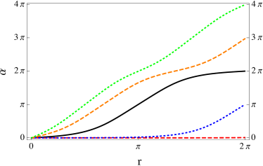
Figure 1: Modulation of the radial mode, $\alpha(r)$, obtained numerically solving Eq. (42) for $q=1$ and $\ell=1/m_{\pi}$ and assuming $\alpha(0)=0$. We report the results obtained with five different values of the integration constant $\eta_{0}$, see Eq.  (44), to match the right boundary condition $\alpha(2\pi)=n\pi$. For $\eta_{0}=0$, red dashed line, the radial mode identically vanishes. With non-vanishing values of $\eta_{0}$ the radial field monotonically grows and the right boundary value $\alpha(2\pi)$ increases with increasing values of $\eta_{0}$.

With increasing values of the lattice size the shape of the $\alpha$ field changes. In Fig. 2 we show the plot of the $\alpha$ field for $n=2$ and three different values of $b$. With increasing values of $b$ the modulation tends to become steeper at $r=\pi$ and flattens at the boundary. For large values of $b$ the system tends to the homogeneous normal phase: the integration constant $\eta_{0}$ decreases with increasing system size and eventually vanishes for asymptotic values of $b$. We have seen above that for $\eta_{0}=0$ one obtains the homogeneous normal phase, however, in this case we have imposed that $\alpha(2\pi)=2\pi$, therefore the $\alpha$ field discontinuously jumps from $0$ to $2\pi$ at $r=\pi$. The fact that the large size case corresponds to the homogeneous normal phase can be seen by combining Eq. (22) and Eq. (38) in

$$\frac{\mu_{I}}{m_{\pi}}=-\frac{p}{b}\,,$$ (48)

and therefore asymptotic values of $b$ correspond to vanishing $\mu_{I}$.

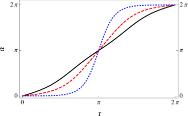
Figure 2: Modulation of the radial mode, $\alpha(r)$, obtained numerically solving Eq. (42) for three different values of the lattice size, see Eq. (22). The solid black line corresponds to $b=0.5$, the dashed red line to $b=1$ and the dotted blue line to $b=2.5$.

For numerical evaluations, we shall hereafter assume the values

$$q=1\,,\quad p=1\,,\quad\ell=1/m_{\pi}\,,\quad\eta_{0}\simeq 0.186\,,$$ (49)

where the last equation implies that $\alpha(2\pi)=2\pi$.

III.1 The energy-momentum tensor

For a given Lagrangian density, $\mathcal{L}$, the energy-momentum tensor is

$$T_{\mu\nu}=2\frac{\partial\mathcal{L}}{\partial g^{\mu\nu}}-g_{\mu\nu}\mathcal{L}\,,$$ (50)

and using the expression in Eq. (III) we obtain the matter contribution

$$T^{\text{m}}_{\mu\nu}= -\frac{f_{\pi}^{2}}{2}\mathrm{Tr}\left(\Sigma_{\mu}\Sigma_{\nu}\right)+\frac{f_{\pi}^{2}}{4}g_{\mu\nu}\mathrm{Tr}\left(\Sigma^{\alpha}\Sigma_{\alpha}\right)$$

$$-g_{\mu\nu}f_{\pi}^{2}m_{\pi}^{2}\cos\alpha\,.$$ (51)

Upon substituting Eq. (36) in Eq. (III.1) and normalizing by subtracting the vacuum energy density, see Eq. (17), we obtain the matter energy-density

$$\epsilon_{\text{m}}= T^{\text{m}}_{00}+f_{\pi}^{2}m_{\pi}^{2}=\frac{f_{\pi}^{2}}{2\ell^{2}}\biggl{(}\eta^{2}+2m_{\pi}^{2}\ell^{2}(1-\cos{\alpha})$$

$$\left.+(2p^{2}\sin^{2}(q\theta)+q^{2})\sin^{2}\alpha\right.\biggl{)}\,.$$

Taking into account the ranges in Eq. (23), the total energy of the system is

$$E_{\text{m}}=\ell^{3}\int drd\theta d\phi\epsilon_{\text{m}}=\pi^{2}f_{\pi}^{2}\ell\int_{0}^{2\pi}\Omega\left(\alpha\right)d\alpha\ ,$$ (52)

where

$$\Omega\left(\alpha\right)=\eta(\alpha)+(q^{2}+p^{2})\frac{\sin^{2}(\alpha)}{\eta(\alpha)}+\ 2m_{\pi}^{2}\ell^{2}\frac{1-\cos(\alpha)}{\eta(\alpha)}\,,$$ (53)

depends on the numerical values of the various constants. For the particular choice in Eq. (49) we obtain

$$E_{\text{m}}=20.5\pi^{2}\frac{f_{\pi}^{2}}{m_{\pi}}\,.$$ (54)

The components of the pressure are instead given by

$$P_{rr}\ = \ \frac{f_{\pi}^{2}}{2\ell^{2}}(\eta^{2}-q^{2}\sin^{2}{\alpha}+2m_{\pi}^{2}\ell^{2}\cos{\alpha})\,,$$

$$P_{\theta\theta}\ = \ \frac{f_{\pi}^{2}}{2\ell^{2}}(-\eta^{2}+q^{2}\sin^{2}{\alpha}+2m_{\pi}^{2}\ell^{2}\cos{\alpha})\,,$$

$$P_{\phi\phi}\ = \ \frac{f_{\pi}^{2}}{2\ell^{2}}\left(2\ell^{2}m_{\pi}^{2}\cos{\alpha}-\eta^{2}-q^{2}\sin^{2}{\alpha}\right.$$

$$\left.+2\sin^{2}(\alpha)\sin^{2}(q\theta)p^{2}\right)\,,$$ (55)

showing that the pressure is not isotropic. This happens because of the space modulation of the $\alpha$ and $\Theta$ fields. When substituting Eq. (44) in Eqs. (55) we obtain

$$P_{rr}\ = \frac{f_{\pi}^{2}}{2\ell^{2}}(\eta_{0}^{2}+2m_{\pi}^{2}\ell^{2})\simeq f_{\pi}^{2}m_{\pi}^{2}\,,$$

$$P_{\theta\theta}\ = \frac{f_{\pi}^{2}}{2\ell^{2}}(2m_{\pi}^{2}\ell^{2}(2\cos\alpha-1)-\eta_{0}^{2})\simeq f_{\pi}^{2}m_{\pi}^{2}(2\cos\alpha-1.01)\ ,$$

$$P_{\phi\phi}\ = \frac{f_{\pi}^{2}}{2\ell^{2}}(2m_{\pi}^{2}\ell^{2}(2\cos\alpha-1)+2\sin^{2}(\alpha)(p^{2}\sin^{2}(q\theta)-q^{2})\ ,$$

$$-\eta_{0}^{2})\simeq f_{\pi}^{2}m_{\pi}^{2}(2\cos\alpha+\sin^{2}(\alpha)(\sin^{2}(\theta)-1)-1.01)\ ,$$ (56)

where the last equalities are obtained using Eq. (49). The fact that the pressure in a certain region of the $(\theta,\phi)$ plane becomes negative follows from the fact that the system is not static, but stationary, therefore cavitation-like phenomena are possible. Finally, we note that

$$T_{0\phi}=-\frac{f_{\pi}^{2}}{\ell^{2}}\sin^{2}{\alpha}\sin^{2}(q\theta)p^{2}=-f_{\pi}^{2}m_{\pi}^{2}\sin^{2}{\alpha}\sin^{2}(\theta)\,,$$ (57)

where the last equation holds for the values in Eq. (49). The presence of a persistent current means that there is a continuous steady energy transfer in the $\phi$ direction, which is due to the presence of a stationary flow.

III.2 Topological charge

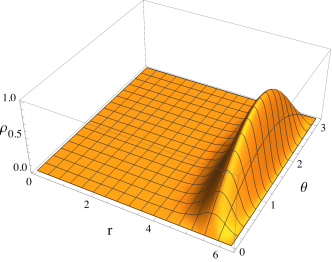
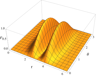
Figure 3: Modulation of the topological density contribution of the matter fields, see Eq. (60), obtained for $n=1$, left hand side, and $n=2$, right hand side. The topological density has been normalized to the value at the maximum.

The topological charge of the solitonic configuration can be written as

$$B_{\text{m}}=\frac{\ell^{3}}{24\pi^{2}}\int drd\theta d\phi\ \rho_{\text{m}}\ \,,$$ (58)

where

$$\rho_{\text{m}}=\epsilon^{ijk}\text{Tr}\left\{\left(\Sigma^{-1}\partial_{i}\Sigma\right)\left(\Sigma^{-1}\partial_{j}\Sigma\right)\left(\Sigma^{-1}\partial_{k}\Sigma\right)\right\}\ ,$$ (59)

is the topological density contribution of the matter fields. The expression in Eq. (59) shows that when the $SU(2)$-valued scalar field $\Sigma$ depends on one or two coordinates, the topological density identically vanishes. Upon substituting Eq. (1) in Eq. (59), the topological density can be rewritten as

$$\rho_{\text{m}}=-12\frac{pq}{\ell^{3}}\sin(q\theta)\sin^{2}(\alpha)\eta$$ (60)

which can be readily integrating noticing that

$$\int dr\sin^{2}(\alpha)\eta=\int d\alpha\sin^{2}\alpha\,,$$ (61)

and since we have imposed the boundary condition in Eq. (46), the topological charge becomes

$$B_{\text{m}}=\begin{cases}-np&\text{if}\quad q\text{ odd}\ ,\\[6.45831pt] 0&\text{if}\quad q\text{ even}\ ,\end{cases}$$ (62)

which clarifies the choice of the $q$ parameter in Eq. (36). We report in Fig. 3 the topological charge densities for the cases with $n=1$, left panel, and $n=2$, right panel. Physically, the topological charge represents the baryonic charge of the system Callan and Witten (1984); Piette and Tchrakian (2000). Therefore, the spatial modulation of the fields is associated with the realization of a non-vanishing baryonic density. With reference to the $q=1$ and $n=2$ case we see from Eqs. (60) and (61) that the two maxima of the topological charge density correspond to $\theta=\pi/2$ and $\alpha=\pi/2$ and $\alpha=3\pi/2$. The normal and condensed phases correspond to values of $\alpha$ in the intervals $[0,\pi/2]$ and $[3\pi/2,2\pi]$, see Eq. (18). These facts suggest that the spatial modulation of the $\alpha$ field in the interval $[0,2\pi]$ describes two (anti)baryons, approximately realized in the interval $[\pi/2,3\pi/2]$, surrounded by a cloud of pions forming a condensate that vanishes at the boundary of the system and reaching its maxima at the places where the the baryonic density takes its maximal values. Systems with a larger baryonic charge correspond to larger values of $n$.

IV Inhomogeneous phase including the gauge field

By including the electromagnetic interaction the matter Lagrangian turns to

$$\mathcal{L}_{\text{m}}= \frac{f_{\pi}^{2}}{2}\left[\partial_{\mu}\alpha\partial^{\mu}\alpha+\sin^{2}{\alpha}\partial_{\mu}\Theta\partial^{\mu}\Theta+2m_{\pi}^{2}\cos\alpha\right.$$

$$\left.+\sin^{2}{\alpha}\sin^{2}{\Theta}(\partial_{\mu}\Phi-2\tilde{A}_{\mu})(\partial^{\mu}\Phi-2\tilde{A}^{\mu})\right]\,,$$ (63)

where $\tilde{A}^{\mu}$ is defined in Eq. (5). From this expression, it is clear that only the $\Phi$ field is minimally coupled to the electromagnetic field. In the following we shall work in the Lorenz gauge $\partial_{\mu}A^{\mu}=0$; by using the particular classical fields in Eq. (36) and

$$A^{\mu}=(u,0,0,u)\,,$$ (64)

the $\alpha(r)$ field decouples and its classical solution satisfies Eq. (39). This means that although the gauge field is generated by the pions, for the particular choice in Eq. (64) it does not back react on the classical fields.

Let us now comment on the particular ansatz in Eq. (64) for the electromagnetic potential. It does not correspond to a particular gauge, but to a particular configuration of the electric and magnetic fields. With this ansatz we have that

$$\bm{E}=-\frac{1}{\ell}(\partial_{r}u,\partial_{\theta}u,0)\,,\qquad\bm{B}=\frac{1}{\ell}(\partial_{\theta}u,-\partial_{r}u,0)\,,$$ (65)

thus the electric and magnetic fields have equal magnitude $|\bm{E}|^{2}=|\bm{B}|^{2}=((\partial_{r}u)^{2}+(\partial_{\theta}u)^{2})/\ell^{2}$ and they are in the $r-\theta$ plane. It remains to be determined the expression of $u$ using the Maxwell equations. From Eq. (8) or Eq. (III) we obtain the electromagnetic current

$$J_{\mu}=-2f_{\pi}^{2}\sin^{2}{\alpha}\sin^{2}(q\theta)(\partial_{\mu}\Phi-2\tilde{A}_{\mu})\,,$$ (66)

therefore the non-vanishing components of the current are

$$J_{0} =-2\frac{f_{\pi}^{2}}{\ell}\sin^{2}(\alpha)\sin^{2}(q\theta)\left(p-2\ell u\right)\ ,$$ (67)

$$J_{\phi} =-J_{0}\,,$$ (68)

where we used Eqs. (22) and (38) with $b=1$, hence Eq. (7) reduces to the one single equation

$$\frac{1}{\ell^{2}}\left(\frac{\partial^{2}}{\partial r^{2}}+\frac{\partial^{2}}{\partial\theta^{2}}\right)u=2\frac{f_{\pi}^{2}}{\ell}\sin^{2}{\alpha}\sin^{2}\Theta\left(p-2\ell u\right)\,,$$ (69)

where we have used Eq. (64) and the Lorenz gauge condition. This expression can be rewritten as a time-independent Schrödinger-like equation in a periodic two-dimensional potential

$$\left(\frac{\partial^{2}}{\partial r^{2}}+\frac{\partial^{2}}{\partial\theta^{2}}\right)\Psi+V\Psi=0\ ,$$ (70)

where

$$\Psi=\frac{p}{\ell}-2u\quad\text{and}\quad V=4f_{\pi}^{2}\ell^{2}\sin^{2}\alpha\sin^{2}(q\theta)\,,$$ (71)

are the wave function and the effective potential, respectively. As boundary condition we assume the simplest one, that is $u=0$ along the whole boundary. The resulting plot of the potential is in Fig. 4, where we have taken $q=1$ and $p=1$. We tried different boundary conditions with a constant shift of the potential at different boundaries, obtaining similar results.

The corresponding electric and magnetic fields are reported in Fig. 5. The electric field is centered at the maxima of the two solitons and decreases its intensity approaching the soliton centers. This shows that the electric field is screened inside the solitons. Similarly, the magnetic field in the right panel of Fig. 5 is screened inside the solitons, where the electromagnetic current reaches its maximum, see Fig. 6. Therefore, there is a form of Meissner screening induced by the persistent electromagnetic current $J^{\phi}$ flowing perpendicularly to the $r-\theta$ plane.

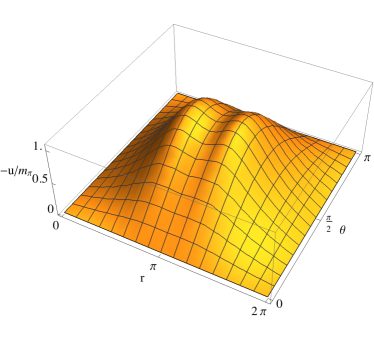
Figure 4: Modulation of the electromagnetic potential as a function of the $r$ and $\theta$ coordinates obtained solving the differential equation (70), where $\Psi=1/\ell-2u$, assuming that $u=0$ at the boundary.

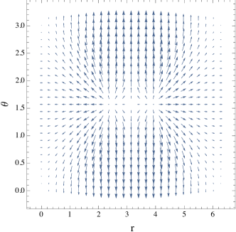
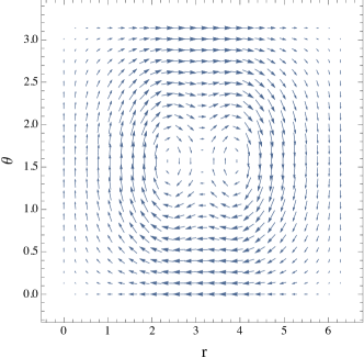
Figure 5: Electric field (left) and magnetic field (right) obtained with the values in Eq. (49) and assuming that the electromagnetic potential vanishes at the boundary.

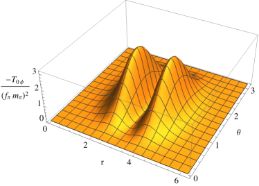
Figure 6: Intensity of the current $T_{0\phi}$ defined in Eq.  (57) flowing along the $\phi$ direction orthogonal to the $r-\theta$ plane. The current is concentrated in the regions where the magnetic field reaches its minimum and the topological matter density as well the energy density reach their maximum values.

Summarizing, we have reduced the three coupled field equations in Eq. (6) and the four coupled Maxwell equations in Eq. (7) to the two differential equations in Eqs. (39) and (70). This has been accomplished by the particular ansatz for the angular classical fields in Eq. (36) and the particularly choice of the gauge field in Eq. (64). This ansatz greatly simplifies the problem. The linear response of the system to the gauge field, Eq. (66), shows that the produced current has the same form of the energy density current in Eq. (57), with the additional gauge field contribution.

Indeed, in the presence of the electromagnetic interaction, there are two additional contributions to the energy-momentum tensor, one is a contribution determined by the minimal coupling with the $\Phi$ field and the other is the pure gauge one. The minimal coupling can be taken into account using Eq. (III.1), where now $\Sigma_{\mu}$ is defined in Eq. (3) and includes the gauge field. The pure gauge contribution has the standard expression

$$T_{\mu\nu}^{\text{em}}=-F_{\mu\alpha}F_{\nu}^{\;\alpha}+\frac{1}{4}F_{\alpha\beta}F^{\alpha\beta}g_{\mu\nu}\,,$$ (72)

which turns in

$$T_{\mu\nu}^{\text{em}}=|\bm{E}|^{2}\left(\begin{array}[]{cccc}1&0&0&1\\ 0&0&0&0\\ 0&0&0&0\\ 1&0&0&1\end{array}\right)\,,$$ (73)

using the particular expression in Eq. (64) of the gauge potential. The energy-density now turns in

$$\epsilon= \frac{f_{\pi}^{2}}{2\ell^{2}}\biggl{(}\eta^{2}+[q^{2}+2(p-2\ell u)^{2}\sin^{2}(q\theta)]\sin^{2}{\alpha}$$

$$\ \ \ +2m_{\pi}^{2}\ell^{2}(1-\cos{\alpha})\biggl{)}+|\bm{E}|^{2}\,,$$ (74)

and taking into account the ranges in Eq. (23), the total energy of the system is

$$E=E_{\text{m}}\ +E_{1}+E_{\text{g}}\,,$$ (75)

where $E_{\text{m}}$ is in Eq. (52) and

$$E_{1}\simeq 17.5\frac{f_{\pi}^{2}}{m_{\pi}}\,,\quad E_{\text{g}}\ \simeq 2.2m_{\pi}\,,$$ (76)

are obtained considering $\ell=1/m_{\pi}$.

The $P_{rr}$ and $P_{\theta\theta}$ pressure components have the same expressions reported in Eq. (55), while

$$P_{\phi\phi}\ = \ \frac{f_{\pi}^{2}}{2\ell^{2}}\left(2\ell^{2}m_{\pi}^{2}\cos{\alpha}-\eta^{2}-q^{2}\sin^{2}{\alpha}\right.$$

$$\left.+2\sin^{2}(q\theta)\sin^{2}(q\theta)(-p+2\ell u)^{2}\right)+|\bm{E}|^{2}\,.$$ (77)

Thus there are additional gauge field contributions only to the pressure in the $\phi$ direction. As before, the energy density and the pressure are not time dependent: the system is stationary with a constant energy transfer in the $\phi$ direction given by

$$T_{0\phi}=-\frac{f_{\pi}^{2}}{\ell}\sin^{2}{\alpha}\sin^{2}(q\theta)(p-2\ell u)^{2}-|\bm{E}|^{2}\ ,$$ (78)

where the last term on the right hand side is the electromagnetic Poynting vector.

For completeness, we notice that when gauging the $U(1)$ symmetry, one should include an additional contribution to the topological charge Callan and Witten (1984); Piette and Tchrakian (2000), which now reads

$$B=\frac{\ell^{3}}{24\pi^{2}}\int drd\theta d\phi\ (\rho_{\text{m}}+\rho_{g})=B_{\text{m}}\ +B_{\text{g}}\ ,$$ (79)

where $B_{\text{m}}$ is defined in Eq. (58). The gauge field contribution

$$\rho_{g}=-i\epsilon^{ijk}\text{Tr}\left\{\partial_{i}\left[3A_{j}\sigma_{3}\left(\Sigma^{-1}\partial_{k}\Sigma+\left(\partial_{k}\Sigma\right)\Sigma^{-1}\right)\right]\right\}\,,$$ (80)

is the Callan-Witten topological charge: it guarantees both the conservation and the gauge invariance of the topological charge. For the considered potential $A_{j}=\delta_{j3}u$, hence this topological density can be written as

$$\rho_{g}=-3i\epsilon^{i3k}\partial_{i}uT_{k}=\frac{3i}{\ell}[\partial_{r}(uT_{2})-\partial_{\theta}(uT_{1})]\,,$$ (81)

where

$$T_{k}=\text{Tr}\left[\sigma_{3}\left(\Sigma^{-1}\partial_{k}\Sigma+\left(\partial_{k}\Sigma\right)\Sigma^{-1}\right)\right]\,,$$ (82)

determine the dependence on the solitonic field. Then, for the considered solitonic configuration we have that

$$B_{g}=\frac{i\ell^{2}}{4\pi}\left\{\int_{0}^{\pi}d\theta\left.uT_{2}\right|_{r=0}^{r=2\pi}-\int_{0}^{2\pi}dr\left.uT_{1}\right|_{\theta=0}^{\theta=\pi}\right\}\,,$$ (83)

where

$$T_{1}=4i\frac{\eta}{\ell}\cos\Theta\ ,\qquad T_{2}=-2i\frac{q}{\ell}\sin 2\alpha\sin\Theta\,.$$ (84)

Since along the boundary the gauge field takes the fixed value $\bar{u}$ and since $\sin 2\alpha(r=2\pi)=\sin 2\alpha(r=0)=0$, see Eq. (46), we readily have that $\left.uT_{2}\right|_{r=0}^{r=2\pi}=0$. Then

$$B_{g}=\frac{\ell}{\pi}\bar{u}(\cos(q\pi)-1)\int_{0}^{2\pi}dr\eta\,.$$ (85)

For $\bar{u}=0$, corresponding to the boundary condition used to obtain Fig. 2, we have that $B_{g}=0$, meaning that there is no contribution of the gauge fields to the topological charge.

For different boundary conditions the topological charge may give a non-vanishing contribution. For instance, for $\bar{u}=p/2\ell$, corresponding to vanishing currents at the boundary, we have that

$$B_{g}=\begin{cases}-np&\text{if}\quad q\text{ odd}\ ,\\[6.45831pt] 0&\text{if}\quad q\text{ even}\ ,\end{cases}$$ (86)

and comparing with Eq. (62), we find that $B=B_{m}+B_{g}=2B_{m}=-2np$, where the last equality holds for $q$ odd.

V Conclusions and Perspectives

We have derived the first analytic example of topologically non-trivial inhomogeneous pion condensates in low-energy QCD in (3+1)-dimensions at finite isospin chemical potential. We have shown that for a particular condensate ansatz, the complete set of field equations both with and without the minimal coupling to the electromagnetic field can be consistently reduced to integrable equations, where the isospin chemical potential can be related to the system size. In these configurations the topological charge does not vanish and it is deeply related to the stationary properties of the system. We find that the energy density $\epsilon_{\text{m}}$, the topological density $\rho_{\text{m}}$ and the currents $J_{0}$, $J_{\phi}$ and $T_{0\phi}$ are constant in the $\phi$ direction while they depend non-trivially on the two spatial coordinates $r$ and $\theta$. The regions of maximal $\rho_{\text{m}}$ are three-dimensional tubes of length $2\pi\ell$ parallel to the $\phi$ direction (the same is true for $\epsilon$ and for the currents), forming a pasta-like phase (see Ravenhall et al. (1983); Hashimoto et al. (1984); Horowitz et al. (2015) and references therein for pasta phases in nuclear physics). It is worth emphasizing that the proposed inhomogeneous phase avoids the Derrick’s scaling argument for the existence of solitonic solutions because it is realized in a finite volume with appropriate non-trivial boundary conditions. Moreover, it is not static, because the $J_{0}$, $J_{\phi}$ and $T_{0\phi}$ currents do not vanish even when the electromagnetic potential vanishes ($u=0$), and are maximal where $\sin^{2}(\alpha)\sin^{2}(q\theta)=1$, see Eqs. (57) and (67), rapidly decreasing far from the peaks. Consequently, these currents cannot be turned off continuously: they are topologically protected. Therefore, these stationary currents are actually supercurrents. If the broken $U(1)$ symmetry is global, they correspond to superfluid currents. If the broken $U(1)$ symmetry is gauged, then they correspond to superconducting currents. Indeed, the typical expression of any supercurrent, see for instance Witten (1985), is

$$\bm{J}\sim\kappa\left(\bm{\nabla}\varphi+{\bm{A}}\right)\ ,$$ (87)

where $\kappa$ is a constant, $\varphi$ is a phase and ${\bm{A}}$ is the $U(1)$ gauge potential. In the standard settings Witten (1985) there is no topological number associated with $\kappa$: the linear stability of the configurations where $\kappa\neq 0$ is established by direct methods (such as linear perturbation theory) and is determined by a control parameter. In the present case, the factor $\sin^{2}(\alpha)\sin^{2}(q\theta)$ in the currents (which plays the role of $\kappa$ in Eq. (87)) is instead topologically protected.

As far as we know, these are the first analytic examples of gauged crystal-like structures in low-energy QCD. The realized configuration can be interpreted as consisting of $n$ baryons embedded in an inhomogeneous pion gas, characterized by the modulation of the $\alpha$, $\Theta$ and $\Phi$ fields. It would be interesting to compare the inhomogeneous and the homogeneous condensates in order to establish which one is more convenient thermodynamically. At a first glance, we could do this explicitly since we can compute the free energy (in a grand canonical ensemble with a chemical potential $\mu_{T}$ associated with the topological charge) both for the homogeneous and for the inhomogeneous condensates. However, the two condensates seem to be realized in different regimes. If we identify the topological charge with the baryonic charge, the inhomogeneous system corresponds to baryons embedded in a pion gas forming a condensate that reaches its maximum values where the baryonic density is larger. On the other hand, the homogeneous phases  attainable within our framework correspond to pure pionic systems. Therefore the two systems correspond to two different grand canonical ensembles. In principle, it is possible to extend chiral perturbation theory including baryons, see for instance Pich (1998); Scherer (2003); Scherer and Schindler (2005), however our procedure is different, because we have introduced baryons as topological objects in a cloud of pions with a non-vanishing isospin asymmetry.

Remarkably, in the presence of a non-vanishing isospin chemical potential it is possible to realize the solitonic configuration eliminating any time dependence of the condensate, thus the boundary conditions are time independent, as well. This is a clear improvement with respect to the case of vanishing $\mu_{I}$, in which the solitonic configuration has been realized with a time dependent $\Phi$ field and then with time dependent boundary conditions Canfora and Maeda (2013); Canfora (2013); Chen et al. (2014); Canfora et al. (2014, 2015); Ayon-Beato et al. (2016); Tallarita and Canfora (2017); Canfora et al. (2017); Giacomini et al. (2018); Astorino et al. (2018); Alvarez et al. (2017); Avilés et al. (2017); Canfora et al. (2018); Canfora (2018); Canfora et al. (2019a, b); Alvarez et al. (2020); Canfora et al. (2020a, b). We have found that when the isospin asymmetry is related to the system size by Eq. (38) any time dependence is eliminated, and only in this case the topologically stable crystalline phase is time independent. It would be interesting to compare our results with those of LQCD simulations, which should realize the condition in Eq. (38) by properly modulating the ratio between the lattice size and the isospin chemical potential. It may well be that the LQCD simulations find that a different configuration is energetically favored. Although stable, the solution we obtained may not correspond to the energetically favored solitonic configuration: to derive our results we have indeed employed a number of simplifying assumptions.

We also notice that in principle one can use numerical techniques to solve the set of differential Eqs. (27), (28) and (29). The comparison with the outcome of these numerical simulations would be quite interesting, as well. In any case, as we have shown, the analytic solutions are not just of academic interest as they disclose relevant physical properties of complex structures that may somehow be hidden in the numerical procedures.

Given the non-trivial crystalline structure of our system, it would also be interesting to investigate the spectrum of its low-energy excitations. While our configurations are protected by their topological charge against decay, the presence of non-trivial pole structures at finite momentum might signal strong fluctuation effects (see eg. Pisarski et al. (2020) for a discussion on how an inhomogeneous chiral phase is turned into a quantum spin liquid by fluctuations). For the modulations considered in this work, we expect at least some of the low-energy excitations to have a phonon-like linear dispersion relation (see Takayama and Oka (1993) for a study in a similar scenario), but a more detailed investigation would definitely be of interest, and we plan to come back to this issue in a future work.

We note that we have derived our results employing leading order $\chi$PT, however the results reported in Alvarez et al. (2020); Canfora et al. (2020a, b), where additional interaction terms have been introduced, strongly suggest that the present construction could be valid even beyond leading order $\chi$PT.

If the crystals discussed in this work are realized in dense stellar objects, they may have various phenomenological effects on their properties. Since a solitonic crystal supports superfluid and/or superconductive flows, it would manifest in a pasta-like structure that influences the thermal transport properties inside the star. Moreover, it should be characterized by a certain rigidity, meaning that deforming the structure should result in a certain energy cost. Thus, for rotating compact stars, it could be relevant for vortex pinning and may be associated with peculiar stellar glitches. Finally, our results suggest that even pion stars, completely made by pions and electrons Carignano et al. (2017); Brandt et al. (2018c); Andersen and Kneschke , could have a rigid crust made by a solitonic crystal. In this case, this phase should manifest not only in peculiar stellar glitches, but it could as well support quadrupolar mass deformations associated with the continuous emission of gravitational waves. We plan to come back on these very interesting issues in a future publication.

Acknowledgements

We thank Rob Pisarski for useful discussions. F. C. has been funded by Fondecyt Grants 1200022. M. L. and A. V. are funded by FONDECYT post-doctoral grant 3190873 and 3200884. The Centro de Estudios Científicos (CECs) is funded by the Chilean Government through the Centers of Excellence Base Financing Program of Conicyt. S. C. has been supported by the MINECO (Spain) under the projects FPA2016-76005-C2-1-P and PID2019- 105614GB-C21, and by the 2017-SGR-929 grant (Catalonia).

References

- Cabibbo and Parisi (1975) N. Cabibbo and G. Parisi, Phys. Lett. 59 B, 67 (1975).
- Gyulassy (2004) M. Gyulassy, in Structure and dynamics of elementary matter. Proceedings, NATO Advanced Study Institute, Camyuva-Kemer, Turkey, September 22-October 2, 2003 (2004) pp. 159–182, arXiv:nucl-th/0403032 [nucl-th] .
- Shuryak (2009) E. Shuryak, Prog. Part. Nucl. Phys. 62, 48 (2009), arXiv:0807.3033 [hep-ph] .
- Satz (2012) H. Satz, Lect. Notes Phys. 841, 1 (2012).
- Shapiro and Teukolsky (1983) S. L. Shapiro and S. A. Teukolsky, Black holes, white dwarfs, and neutron stars: The physics of compact objects (1983).
- Glendenning (1997) N. K. Glendenning, Compact stars: Nuclear physics, particle physics, and general relativity (1997).
- Brambilla et al. (2014) N. Brambilla et al., Eur. Phys. J. C74, 2981 (2014), arXiv:1404.3723 [hep-ph] .
- Smit (2002) J. Smit, Cambridge Lect. Notes Phys. 15, 1 (2002).
- Gattringer and Lang (2010) C. Gattringer and C. B. Lang, Lect. Notes Phys. 788, 1 (2010).
- Muroya et al. (2003) S. Muroya, A. Nakamura, C. Nonaka, and T. Takaishi, Prog. Theor. Phys. 110, 615 (2003), arXiv:hep-lat/0306031 [hep-lat] .
- Schmidt (2006) C. Schmidt, Proceedings, 24th International Symposium on Lattice Field Theory (Lattice 2006): Tucson, USA, July 23-28, 2006, PoS LAT2006, 021 (2006), arXiv:hep-lat/0610116 [hep-lat] .
- de Forcrand (2009) P. de Forcrand, Proceedings, 27th International Symposium on Lattice field theory (Lattice 2009): Beijing, P.R. China, July 26-31, 2009, PoS LAT2009, 010 (2009), arXiv:1005.0539 [hep-lat] .
- Philipsen (2013) O. Philipsen, Prog. Part. Nucl. Phys. 70, 55 (2013), arXiv:1207.5999 [hep-lat] .
- Aarts (2016) G. Aarts, Proceedings, 13th International Workshop on Hadron Physics: Angra dos Reis, Rio de Janeiro, Brazil, March 22-27, 2015, J. Phys. Conf. Ser. 706, 022004 (2016), arXiv:1512.05145 [hep-lat] .
- Alford et al. (1999) M. G. Alford, A. Kapustin, and F. Wilczek, Phys. Rev. D 59, 054502 (1999), arXiv:hep-lat/9807039 [hep-lat] .
- Kogut and Sinclair (2002a) J. B. Kogut and D. K. Sinclair, Phys. Rev. D66, 014508 (2002a), arXiv:hep-lat/0201017 [hep-lat] .
- Kogut and Sinclair (2002b) J. B. Kogut and D. K. Sinclair, Phys. Rev. D 66, 034505 (2002b), arXiv:hep-lat/0202028 [hep-lat] .
- Kogut and Sinclair (2004) J. B. Kogut and D. K. Sinclair, Phys. Rev. D70, 094501 (2004), arXiv:hep-lat/0407027 [hep-lat] .
- Beane et al. (2008) S. R. Beane, W. Detmold, T. C. Luu, K. Orginos, M. J. Savage, and A. Torok, Phys. Rev. Lett. 100, 082004 (2008), arXiv:0710.1827 [hep-lat] .
- Detmold et al. (2008a) W. Detmold, M. J. Savage, A. Torok, S. R. Beane, T. C. Luu, K. Orginos, and A. Parreno, Phys. Rev. D78, 014507 (2008a), arXiv:0803.2728 [hep-lat] .
- Detmold et al. (2008b) W. Detmold, K. Orginos, M. J. Savage, and A. Walker-Loud, Phys. Rev. D 78, 054514 (2008b), arXiv:0807.1856 [hep-lat] .
- Detmold and Smigielski (2011) W. Detmold and B. Smigielski, Phys. Rev. D84, 014508 (2011), arXiv:1103.4362 [hep-lat] .
- Detmold et al. (2012) W. Detmold, K. Orginos, and Z. Shi, Phys. Rev. D 86, 054507 (2012), arXiv:1205.4224 [hep-lat] .
- Endrödi (2014) G. Endrödi, Phys. Rev. D 90, 094501 (2014), arXiv:1407.1216 [hep-lat] .
- Janssen et al. (2016) O. Janssen, M. Kieburg, K. Splittorff, J. J. M. Verbaarschot, and S. Zafeiropoulos, Phys. Rev. D93, 094502 (2016), arXiv:1509.02760 [hep-lat] .
- Brandt and Endrodi (2016) B. B. Brandt and G. Endrodi, Proceedings, 34th International Symposium on Lattice Field Theory (Lattice 2016): Southampton, UK, July 24-30, 2016, PoS LATTICE2016, 039 (2016), arXiv:1611.06758 [hep-lat] .
- Brandt and Endrodi (2019) B. B. Brandt and G. Endrodi, Phys. Rev. D99, 014518 (2019), arXiv:1810.11045 [hep-lat] .
- Brandt et al. (2018a) B. B. Brandt, G. Endrodi, and S. Schmalzbauer, Proceedings, 35th International Symposium on Lattice Field Theory (Lattice 2017): Granada, Spain, June 18-24, 2017, EPJ Web Conf. 175, 07020 (2018a), arXiv:1709.10487 [hep-lat] .
- Brandt et al. (2018b) B. B. Brandt, G. Endrodi, and S. Schmalzbauer (2018) arXiv:1811.06004 [hep-lat] .
- Baym and Campbell (1978) G. Baym and D. K. Campbell, in Mesons in Nuclei, 1979 (1978) p. 1031.
- Kaplan and Nelson (1986) D. B. Kaplan and A. E. Nelson, Phys. Lett. B175, 57 (1986).
- Dominguez et al. (1994) C. Dominguez, M. Loewe, and J. Rojas, Phys.Lett. B320, 377 (1994).
- Son and Stephanov (2001) D. Son and M. A. Stephanov, Phys. Rev. Lett. 86, 592 (2001), arXiv:hep-ph/0005225 [hep-ph] .
- Kogut and Toublan (2001) J. Kogut and D. Toublan, Phys. Rev. D 64, 034007 (2001), arXiv:hep-ph/0103271 [hep-ph] .
- Birse et al. (2001) M. C. Birse, T. D. Cohen, and J. A. McGovern, Phys. Lett. B516, 27 (2001), arXiv:hep-ph/0104282 [hep-ph] .
- Splittorff et al. (2002) K. Splittorff, D. Toublan, and J. J. M. Verbaarschot, Nucl. Phys. B639, 524 (2002), arXiv:hep-ph/0204076 [hep-ph] .
- Loewe and Villavicencio (2003) M. Loewe and C. Villavicencio, Phys.Rev. D67, 074034 (2003), arXiv:hep-ph/0212275 [hep-ph] .
- Loewe and Villavicencio (2004) M. Loewe and C. Villavicencio, Phys.Rev. D70, 074005 (2004), arXiv:hep-ph/0404232 [hep-ph] .
- Loewe and Villavicencio (2011) M. Loewe and C. Villavicencio, (2011), arXiv:1107.3859 [hep-ph] .
- Mammarella and Mannarelli (2015) A. Mammarella and M. Mannarelli, Phys. Rev. D 92, 085025 (2015), arXiv:1507.02934 [hep-ph] .
- Adhikari et al. (2015) P. Adhikari, T. D. Cohen, and J. Sakowitz, Phys. Rev. C 91, 045202 (2015), arXiv:1501.02737 [nucl-th] .
- Carignano et al. (2016) S. Carignano, A. Mammarella, and M. Mannarelli, Phys. Rev. D 93, 051503 (2016), arXiv:1602.01317 [hep-ph] .
- Loewe et al. (2016) M. Loewe, A. Raya, and C. Villavicencio, (2016), arXiv:1610.05751 [hep-ph] .
- Carignano et al. (2017) S. Carignano, L. Lepori, A. Mammarella, M. Mannarelli, and G. Pagliaroli, Eur. Phys. J. A 53, 35 (2017), arXiv:1610.06097 [hep-ph] .
- Adhikari (2019) P. Adhikari, Phys. Lett. B 790, 211 (2019), arXiv:1810.03663 [nucl-th] .
- Lepori and Mannarelli (2019) L. Lepori and M. Mannarelli, Phys. Rev. D99, 096011 (2019), arXiv:1901.07488 [hep-ph] .
- Adhikari et al. (2019) P. Adhikari, J. O. Andersen, and P. Kneschke, (2019), arXiv:1904.03887 [hep-ph] .
- Tawfik et al. (2019) A. N. Tawfik, A. M. Diab, M. T. Ghoneim, and H. Anwer, (2019), arXiv:1904.09890 [hep-ph] .
- Mishustin et al. (2019) I. N. Mishustin, D. V. Anchishkin, L. M. Satarov, O. S. Stashko, and H. Stoecker, (2019), arXiv:1905.09567 [nucl-th] .
- Adhikari and Andersen (2020a) P. Adhikari and J. O. Andersen, Phys. Lett. B 804, 135352 (2020a), arXiv:1909.01131 [hep-ph] .
- Adhikari and Andersen (2020b) P. Adhikari and J. O. Andersen, JHEP 06, 170 (2020b), arXiv:1909.10575 [hep-ph] .
- Adhikari and Nguyen (2020) P. Adhikari and H. Nguyen, (2020), arXiv:2002.04052 [hep-ph] .
- Adhikari and Andersen (2020c) P. Adhikari and J. O. Andersen, (2020c), arXiv:2003.12567 [hep-ph] .
- Agasian (2020) N. Agasian, JETP Lett. 111, 201 (2020).
- Adhikari et al. (2021) P. Adhikari, J. O. Andersen, and M. A. Mojahed, Eur. Phys. J. C 81, 173 (2021), arXiv:2010.13655 [hep-ph] .
- Barducci et al. (1990) A. Barducci, R. Casalbuoni, S. De Curtis, R. Gatto, and G. Pettini, Phys. Rev. D 42, 1757 (1990).
- Toublan and Kogut (2003) D. Toublan and J. B. Kogut, Phys. Lett. B564, 212 (2003), arXiv:hep-ph/0301183 [hep-ph] .
- Barducci et al. (2004) A. Barducci, R. Casalbuoni, G. Pettini, and L. Ravagli, Phys. Rev. D 69, 096004 (2004), arXiv:hep-ph/0402104 [hep-ph] .
- Barducci et al. (2005) A. Barducci, R. Casalbuoni, G. Pettini, and L. Ravagli, Phys. Rev. D 71, 016011 (2005), arXiv:hep-ph/0410250 [hep-ph] .
- He et al. (2005) L.-Y. He, M. Jin, and P.-F. Zhuang, Phys. Rev. D 71, 116001 (2005), arXiv:hep-ph/0503272 [hep-ph] .
- Ebert and Klimenko (2006a) D. Ebert and K. G. Klimenko, J. Phys. G32, 599 (2006a), arXiv:hep-ph/0507007 [hep-ph] .
- Ebert and Klimenko (2006b) D. Ebert and K. G. Klimenko, Eur. Phys. J. C46, 771 (2006b), arXiv:hep-ph/0510222 [hep-ph] .
- Mukherjee et al. (2007) S. Mukherjee, M. G. Mustafa, and R. Ray, Phys. Rev. D75, 094015 (2007), arXiv:hep-ph/0609249 [hep-ph] .
- He and Zhuang (2005) L. He and P. Zhuang, Phys. Lett. B615, 93 (2005), arXiv:hep-ph/0501024 [hep-ph] .
- He et al. (2006) L. He, M. Jin, and P. Zhuang, Phys. Rev. D74, 036005 (2006), arXiv:hep-ph/0604224 [hep-ph] .
- Sun et al. (2007) G.-f. Sun, L. He, and P. Zhuang, Phys. Rev. D75, 096004 (2007), arXiv:hep-ph/0703159 [hep-ph] .
- Andersen and Kyllingstad (2009) J. O. Andersen and L. Kyllingstad, J. Phys. G37, 015003 (2009), arXiv:hep-ph/0701033 [hep-ph] .
- Abuki et al. (2008) H. Abuki, M. Ciminale, R. Gatto, N. D. Ippolito, G. Nardulli, and M. Ruggieri, Phys. Rev. D78, 014002 (2008), arXiv:0801.4254 [hep-ph] .
- Abuki et al. (2009) H. Abuki, R. Anglani, R. Gatto, M. Pellicoro, and M. Ruggieri, Phys. Rev. D79, 034032 (2009), arXiv:0809.2658 [hep-ph] .
- Mu et al. (2010) C.-f. Mu, L.-y. He, and Y.-x. Liu, Phys. Rev. D82, 056006 (2010).
- Xia et al. (2013) T. Xia, L. He, and P. Zhuang, Phys. Rev. D88, 056013 (2013), arXiv:1307.4622 [hep-ph] .
- Xia and Zhuang (2014) T. Xia and P. Zhuang, (2014), arXiv:1411.6713 [hep-ph] .
- Chao et al. (2018) J. Chao, M. Huang, and A. Radzhabov, (2018), arXiv:1805.00614 [hep-ph] .
- Khunjua et al. (2019a) T. G. Khunjua, K. G. Klimenko, and R. N. Zhokhov, JHEP 06, 006 (2019a), arXiv:1901.02855 [hep-ph] .
- Khunjua et al. (2019b) T. Khunjua, K. Klimenko, and R. Zhokhov, Symmetry 11, 778 (2019b).
- Avancini et al. (2019) S. S. Avancini, A. Bandyopadhyay, D. C. Duarte, and R. L. S. Farias, (2019), arXiv:1907.09880 [hep-ph] .
- Lu et al. (2019) Z.-Y. Lu, C.-J. Xia, and M. Ruggieri, (2019), arXiv:1907.11497 [hep-ph] .
- Cao and He (2019) G. Cao and L. He, Phys. Rev. D 100, 094015 (2019), arXiv:1910.02728 [nucl-th] .
- Khunjua et al. (2020a) T. Khunjua, K. Klimenko, and R. Zhokhov, JHEP 06, 148 (2020a), arXiv:2003.10562 [hep-ph] .
- Khunjua et al. (2020b) T. Khunjua, K. Klimenko, and R. Zhokhov, (2020b), arXiv:2005.05488 [hep-ph] .
- Mao (2020) S. Mao, (2020), arXiv:2009.11550 [nucl-th] .
- Mannarelli (2019) M. Mannarelli, Particles 2, 411 (2019), arXiv:1908.02042 [hep-ph] .
- Fukushima and Hatsuda (2011) K. Fukushima and T. Hatsuda, Rept. Prog. Phys. 74, 014001 (2011), arXiv:1005.4814 [hep-ph] .
- Anglani et al. (2014) R. Anglani, R. Casalbuoni, M. Ciminale, N. Ippolito, R. Gatto, et al., Rev. Mod. Phys. 86, 509 (2014), arXiv:1302.4264 [hep-ph] .
- Buballa and Carignano (2015) M. Buballa and S. Carignano, Prog. Part. Nucl. Phys. 81, 39 (2015), arXiv:1406.1367 [hep-ph] .
- Harada et al. (2015) M. Harada, H. K. Lee, Y.-L. Ma, and M. Rho, Phys. Rev. D 91, 096011 (2015), arXiv:1502.02508 [hep-ph] .
- Kaplunovsky et al. (2015) V. Kaplunovsky, D. Melnikov, and J. Sonnenschein, Mod. Phys. Lett. B 29, 1540052 (2015), arXiv:1501.04655 [hep-th] .
- Park et al. (2019) B.-Y. Park, W.-G. Paeng, and V. Vento, Nucl. Phys. A 989, 231 (2019), arXiv:1904.04483 [hep-ph] .
- Basar and Dunne (2008a) G. Basar and G. V. Dunne, Phys. Rev. Lett. 100, 200404 (2008a), arXiv:0803.1501 [hep-th] .
- Basar and Dunne (2008b) G. Basar and G. V. Dunne, Phys. Rev. D78, 065022 (2008b), arXiv:0806.2659 [hep-th] .
- Basar et al. (2009) G. Basar, G. V. Dunne, and M. Thies, Phys. Rev. D79, 105012 (2009), arXiv:0903.1868 [hep-th] .
- Thies (2004) M. Thies, Phys. Rev. D69, 067703 (2004), arXiv:hep-th/0308164 [hep-th] .
- Bringoltz (2009) B. Bringoltz, Phys. Rev. D79, 125006 (2009), arXiv:0901.4035 [hep-lat] .
- Nickel (2009) D. Nickel, Phys.Rev. D80, 074025 (2009), arXiv:0906.5295 [hep-ph] .
- Karbstein and Thies (2007) F. Karbstein and M. Thies, Phys. Rev. D75, 025003 (2007), arXiv:hep-th/0610243 [hep-th] .
- Takayama and Oka (1993) K. Takayama and M. Oka, Nucl. Phys. A551, 637 (1993).
- Schon and Thies (2000) V. Schon and M. Thies, Phys. Rev. D62, 096002 (2000), arXiv:hep-th/0003195 [hep-th] .
- Gubina et al. (2012) N. Gubina, K. Klimenko, S. Kurbanov, and V. Zhukovsky, Phys. Rev. D 86, 085011 (2012), arXiv:1206.2519 [hep-ph] .
- Andersen and Kneschke (2018) J. O. Andersen and P. Kneschke, Phys. Rev. D97, 076005 (2018), arXiv:1802.01832 [hep-ph] .
- Brauner and Yamamoto (2017) T. Brauner and N. Yamamoto, JHEP 04, 132 (2017), arXiv:1609.05213 [hep-ph] .
- Huang et al. (2018) X.-G. Huang, K. Nishimura, and N. Yamamoto, JHEP 02, 069 (2018), arXiv:1711.02190 [hep-ph] .
- Gross and Neveu (1974) D. J. Gross and A. Neveu, Phys.Rev. D10, 3235 (1974).
- Dashen et al. (1975) R. F. Dashen, B. Hasslacher, and A. Neveu, Phys. Rev. D12, 2443 (1975).
- Shei (1976) S.-S. Shei, Phys. Rev. D14, 535 (1976).
- Feinberg and Zee (1997) J. Feinberg and A. Zee, Phys. Rev. D56, 5050 (1997), arXiv:cond-mat/9603173 [cond-mat] .
- Schroers (1995) B. J. Schroers, Phys. Lett. B356, 291 (1995), arXiv:hep-th/9506004 [hep-th] .
- Arthur and Tchrakian (1996) K. Arthur and D. H. Tchrakian, Phys. Lett. B378, 187 (1996), arXiv:hep-th/9601053 [hep-th] .
- Gladikowski et al. (1996) J. Gladikowski, B. M. A. G. Piette, and B. J. Schroers, Phys. Rev. D53, 844 (1996), arXiv:hep-th/9506099 [hep-th] .
- Cho and Kimm (1995) Y. M. Cho and K. Kimm, Phys. Rev. D52, 7325 (1995).
- Loginov and Gauzshtein (2018) A. Yu. Loginov and V. V. Gauzshtein, Phys. Lett. B784, 112 (2018), arXiv:1901.04471 [hep-th] .
- Adam et al. (2015) C. Adam, C. Naya, T. Romanczukiewicz, J. Sanchez-Guillen, and A. Wereszczynski, JHEP 05, 155 (2015), arXiv:1501.03817 [hep-th] .
- Adam et al. (2014) C. Adam, T. Romanczukiewicz, J. Sanchez-Guillen, and A. Wereszczynski, JHEP 11, 095 (2014), arXiv:1405.5215 [hep-th] .
- Alonso-Izquierdo et al. (2015) A. Alonso-Izquierdo, W. G. Fuertes, and J. Mateos Guilarte, JHEP 02, 139 (2015), arXiv:1409.8419 [hep-th] .
- Chimento et al. (2018) S. Chimento, T. Ortin, and A. Ruipérez, JHEP 05, 107 (2018), arXiv:1802.03332 [hep-th] .
- Baym et al. (1982) G. Baym, B. L. Friman, and G. Grinstein, Nucl. Phys. B210, 193 (1982).
- Skyrme (1961a) T. H. R. Skyrme, Proc. Roy. Soc. Lond. A260, 127 (1961a).
- Skyrme (1961b) T. H. R. Skyrme, Proc. Roy. Soc. Lond. A262, 237 (1961b).
- Skyrme (1962) T. H. R. Skyrme, Lewes Center for Physics: An East Coast Summer Physics Center Lewes, Del., June 2-July 27, 1984, Nucl. Phys. 31, 556 (1962), [,13(1962)].
- Derrick (1964) G. H. Derrick, J. Math. Phys. 5, 1252 (1964).
- Canfora and Maeda (2013) F. Canfora and H. Maeda, Phys. Rev. D87, 084049 (2013), arXiv:1302.3232 [gr-qc] .
- Canfora (2013) F. Canfora, Phys. Rev. D88, 065028 (2013), arXiv:1307.0211 [hep-th] .
- Chen et al. (2014) S. Chen, Y. Li, and Y. Yang, Phys. Rev. D 89, 025007 (2014).
- Canfora et al. (2014) F. Canfora, F. Correa, and J. Zanelli, Phys. Rev. D90, 085002 (2014), arXiv:1406.4136 [hep-th] .
- Canfora et al. (2015) F. Canfora, M. Di Mauro, M. A. Kurkov, and A. Naddeo, Eur. Phys. J. C75, 443 (2015), arXiv:1508.07055 [hep-th] .
- Ayon-Beato et al. (2016) E. Ayon-Beato, F. Canfora, and J. Zanelli, Phys. Lett. B752, 201 (2016), arXiv:1509.02659 [gr-qc] .
- Tallarita and Canfora (2017) G. Tallarita and F. Canfora, Nucl. Phys. B921, 394 (2017), arXiv:1706.01397 [hep-th] .
- Canfora et al. (2017) F. Canfora, A. Paliathanasis, T. Taves, and J. Zanelli, Phys. Rev. D95, 065032 (2017), arXiv:1703.04860 [hep-th] .
- Giacomini et al. (2018) A. Giacomini, M. Lagos, J. Oliva, and A. Vera, Phys. Lett. B783, 193 (2018), arXiv:1708.06863 [hep-th] .
- Astorino et al. (2018) M. Astorino, F. Canfora, M. Lagos, and A. Vera, Phys. Rev. D97, 124032 (2018), arXiv:1805.12252 [hep-th] .
- Alvarez et al. (2017) P. D. Alvarez, F. Canfora, N. Dimakis, and A. Paliathanasis, Phys. Lett. B773, 401 (2017), arXiv:1707.07421 [hep-th] .
- Avilés et al. (2017) L. Avilés, F. Canfora, N. Dimakis, and D. Hidalgo, Phys. Rev. D96, 125005 (2017), arXiv:1711.07408 [hep-th] .
- Canfora et al. (2018) F. Canfora, M. Lagos, S. H. Oh, J. Oliva, and A. Vera, Phys. Rev. D98, 085003 (2018), arXiv:1809.10386 [hep-th] .
- Canfora (2018) F. Canfora, Eur. Phys. J. C78, 929 (2018), arXiv:1807.02090 [hep-th] .
- Canfora et al. (2019a) F. Canfora, N. Dimakis, and A. Paliathanasis, Eur. Phys. J. C79, 139 (2019a), arXiv:1902.01563 [hep-th] .
- Canfora et al. (2019b) F. Canfora, S. H. Oh, and A. Vera, Eur. Phys. J. C 79, 485 (2019b), arXiv:1905.12818 [hep-th] .
- Alvarez et al. (2020) P. D. Alvarez, S. L. Cacciatori, F. Canfora, and B. L. Cerchiai, Phys. Rev. D 101, 125011 (2020), arXiv:2005.11301 [hep-th] .
- Canfora et al. (2020a) F. Canfora, M. Lagos, and A. Vera, Eur. Phys. J. C 80, 697 (2020a), arXiv:2007.11543 [hep-th] .
- Canfora et al. (2020b) F. Canfora, A. Giacomini, M. Lagos, S. H. Oh, and A. Vera, (2020b), arXiv:2001.11910 [hep-th] .
- Weinberg (1979) S. Weinberg, Physica A 96, 327 (1979).
- Gasser and Leutwyler (1984) J. Gasser and H. Leutwyler, Ann. Phys. 158, 142 (1984).
- Georgi (1984) H. Georgi, Weak Interactions and Modern Particle Theory (1984).
- Leutwyler (1994) H. Leutwyler, Ann. Phys. 235, 165 (1994), arXiv:hep-ph/9311274 [hep-ph] .
- Ecker (1995) G. Ecker, Prog. Part. Nucl. Phys. 35, 1 (1995), arXiv:hep-ph/9501357 [hep-ph] .
- Leutwyler (1997) H. Leutwyler, Helv. Phys. Acta 70, 275 (1997), arXiv:hep-ph/9609466 [hep-ph] .
- Pich (1998) A. Pich, in Probing the standard model of particle interactions. Proceedings, Summer School in Theoretical Physics, NATO Advanced Study Institute, 68th session, Les Houches, France, July 28-September 5, 1997. Pt. 1, 2 (1998) pp. 949–1049, arXiv:hep-ph/9806303 [hep-ph] .
- Scherer (2003) S. Scherer, Adv. Nucl. Phys. 27, 277 (2003), arXiv:hep-ph/0210398 [hep-ph] .
- Scherer and Schindler (2005) S. Scherer and M. R. Schindler, (2005), arXiv:hep-ph/0505265 [hep-ph] .
- Kogut et al. (1999) J. B. Kogut, M. A. Stephanov, and D. Toublan, Phys. Lett. B 464, 183 (1999), arXiv:hep-ph/9906346 [hep-ph] .
- Kogut et al. (2000) J. B. Kogut, M. A. Stephanov, D. Toublan, J. J. M. Verbaarschot, and A. Zhitnitsky, Nucl. Phys. B 582, 477 (2000), arXiv:hep-ph/0001171 [hep-ph] .
- Hands et al. (2000) S. Hands, I. Montvay, S. Morrison, M. Oevers, L. Scorzato, and J. Skullerud, Eur. Phys. J. C 17, 285 (2000), arXiv:hep-lat/0006018 [hep-lat] .
- Kogut et al. (2001) J. B. Kogut, D. K. Sinclair, S. J. Hands, and S. E. Morrison, Phys. Rev. D 64, 094505 (2001), arXiv:hep-lat/0105026 [hep-lat] .
- Brauner (2006) T. Brauner, Mod. Phys. Lett. A 21, 559 (2006), arXiv:hep-ph/0601010 [hep-ph] .
- Braguta et al. (2016) V. V. Braguta, E. M. Ilgenfritz, A. Yu. Kotov, A. V. Molochkov, and A. A. Nikolaev, Phys. Rev. D 94, 114510 (2016), arXiv:1605.04090 [hep-lat] .
- Adhikari et al. (2018) P. Adhikari, S. B. Beleznay, and M. Mannarelli, Eur. Phys. J. C 78, 441 (2018), arXiv:1803.00490 [hep-th] .
- Callan and Witten (1984) C. G. Callan, Jr. and E. Witten, Nucl. Phys. B239, 161 (1984).
- Piette and Tchrakian (2000) B. M. A. G. Piette and D. H. Tchrakian, Phys. Rev. D62, 025020 (2000), arXiv:hep-th/9709189 [hep-th] .
- Ravenhall et al. (1983) D. G. Ravenhall, C. J. Pethick, and J. R. Wilson, Phys. Rev. Lett. 50, 2066 (1983).
- Hashimoto et al. (1984) M. Hashimoto, H. Seki, and M. Yamada, Progress of Theoretical Physics 71, 320 (1984), https://academic.oup.com/ptp/article-pdf/71/2/320/5459325/71-2-320.pdf .
- Horowitz et al. (2015) C. Horowitz, D. Berry, C. Briggs, M. Caplan, A. Cumming, and A. Schneider, Phys. Rev. Lett. 114, 031102 (2015), arXiv:1410.2197 [astro-ph.HE] .
- Witten (1985) E. Witten, Nucl. Phys. B249, 557 (1985).
- Pisarski et al. (2020) R. D. Pisarski, A. M. Tsvelik, and S. Valgushev, Phys. Rev. D 102, 016015 (2020), arXiv:2005.10259 [hep-ph] .
- Brandt et al. (2018c) B. B. Brandt, G. Endrődi, E. S. Fraga, M. Hippert, J. Schaffner-Bielich, and S. Schmalzbauer, Phys. Rev. D 98, 094510 (2018c).
- (163) J. O. Andersen and P. Kneschke, arXiv:1807.08951 [hep-ph] .