Ensemble of Discriminators for Domain Adaptation
in Multiple Sound Source 2D Localization

Abstract

This paper introduces an ensemble of discriminators that improves the accuracy of a domain adaptation technique for the localization of multiple sound sources. Recently, deep neural networks have led to promising results for this task, yet they require a large amount of labeled data for training. Recording and labeling such datasets is very costly, especially because data needs to be diverse enough to cover different acoustic conditions. In this paper, we leverage acoustic simulators to inexpensively generate labeled training samples. However, models trained on synthetic data tend to perform poorly with real-world recordings due to the domain mismatch. For this, we explore two domain adaptation methods using adversarial learning for sound source localization which use labeled synthetic data and unlabeled real data. We propose a novel ensemble approach that combines discriminators applied at different feature levels of the localization model. Experiments show that our ensemble discrimination method significantly improves the localization performance without requiring any label from the real data.

Index Terms: adversarial domain adaptation, 2D sound localization, multiple sound sources, deep learning

1 Introduction

Sound source localization (SSL) aims at estimating a pose/location of sound sources. With an increasing popularity in installing smart speakers in home environments, source location provides additional knowledge that could enable a variety of applications such as monitoring human activities in daily life [1], speech enhancement [2] and human-robot interaction [3]. SSL is an active research topic for which various signal processing methods have been proposed [3, 4]. These data-independent methods work well under strict assumptions [4], e.g. high signal-to-noise ratio, known number of sources, low reverberation, etc. Such ideal conditions hardly hold true in real-world applications and usually require special treatments [5, 6, 7, 8]. Recently, data-driven approaches and in particular deep learning have outperformed classical signal processing methods for various audio tasks [9, 10] including SSL [11, 12, 13, 14, 15, 16, 17, 18].

Multiple network architectures have been proposed to localize sound sources. An advantage of these methods, apart from their ability to adapt to challenging acoustic conditions and microphone configurations, is that they can be trained to solve multiple tasks at the same time like simultaneous localization and classification of sounds [13]. However, a significant downside is that they require lots of training data, which is expensive to gather and label [19, 20] Acoustic simulators are an appealing solution as they can abundantly generate high-quality labeled datasets. However, models trained on synthetic data as a source domain can suffer from a critical drop in performance when exposed to real-world data as the target domain. This is due to acoustic conditions which are outside the distribution of the synthetic training dataset [21, 22], thus resulting in a domain shift [23].

Recently, there have been several works about domain adaptation for SSL. For example, [24, 25] proposed unsupervised methods using entropy minimization of the localization output. However, such methods are not suitable to our problem because entropy minimization encourages the prediction of only a single source whereas we must cater to multiple outputs. In this context, [19] has proposed two adaptation methods compatible for multiple SSL; (m₁) a weakly supervised method in which the number of sources is provided for real-world data; (m₂) an unsupervised method based on Domain Adversarial Neural Networks (DANN) [26] which intends to align latent feature distributions for synthetic and real-world domains by adding a discriminative model at a certain feature level of the localization model. They reported that m₁ increased the localization performance whereas m₂ did not yield significant improvements. However, adversarial methods such as [26] are popular outside SSL. For example, [27] proposes an adversarial domain adaptation method for the semantic segmentation problem in computer vision. Moreover, similar approaches have been successfully applied to other audio tasks such as Acoustic Scene Classification (ASC) [28] and Sound Event Detection (SED) [29]. Since it is not clear whether adversarial methods are suitable for SSL, we also present extensive experiments with such methods.

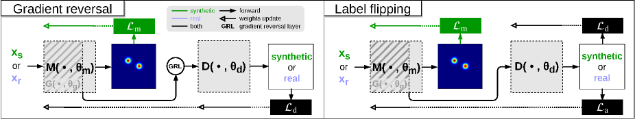
Figure 1: Outline of the domain adaptation framework for the two studied methods with intermediate discrimination.

In this paper, we tackle the lack-of-data problem for 2D multiple SSL by leveraging simulation to cheaply generate a large amount of labeled data. We then address the domain shift issue by training the localization model in such a way that the knowledge is transferable to the real-world. The main contributions of this work are: (a) We explore two domain adaptation methods based on adversarial learning: gradient reversal and label flipping. We analyse the difference of the two methods and show that they work for multiple SSL. (b) We propose a novel ensemble discrimination method for domain adaptation in SSL. It consists of placing a discriminator at different levels of the localization model: the intermediate and output space. (c) We evaluate our proposed method extensively on data captured from a real environment. For each method, we ensure the consistency of the results by performing the experiments on different random seeds and reporting their mean and variance. Through our experiments, we show that our ensemble discrimination method outperforms the standard adversarial learning approaches and can perform similarly to localization models that were trained in a supervised fashion on labeled real-world data. To the best of our knowledge, this is the first successful attempt in tackling domain adaptation for multiple SSL that does not require any label from the real-world data.

2 Domain Adaptation for Multiple Sound Source 2D Localization

Supervised learning relies on the assumption that data is independently and identically distributed. So training a deep learning model on synthetic data and testing without further training on real-world data usually results in a performance drop due to the distributions being different, that is, the simulator is not perfect. However, improving the simulation model is often too difficult. A more practical approach is randomizing the simulator parameters [30]. This expands the source domain in the hopes of covering the target domain. In acoustic simulators, parameters such as noise and reverberation can be randomized to get this effect. However, this can still be insufficient for more difficult tasks [30]. Assuming we can no longer improve the simulator and the model performance on real data is still insufficient, we need to use domain adaptation techniques [23]. Such methods consists in making the model aware of the domain mismatch during the training process. This paper focuses on these methods, and in particular those that use adversarial learning.

To start, we formally describe the base task of learning to predict the location of multiple simultaneous sound sources in a 2D horizontal plane. First, we extract spectral features $\mathcal{X}$ from the sound recorded by a set of microphones. Then, a localization model $M$, with parameters $\theta_{m}$, is trained to map spectral features to a localization heatmap $\mathcal{Y}$: a discretized grid with Gaussian distributions centered at the source locations. Training the model amounts to solving:

$$\min_{\theta_{m}}\sum_{x\in\mathcal{X}}\mathcal{L}_{\text{m}}(M(x),y),$$ (1)

where $y\in\mathcal{Y}$ and the mean squared error (MSE) is used as the localization model loss ($\mathcal{L}_{\text{m}}$). Such a framework was introduced in [20], to which readers are referred for further details.

We wish to augment (1) so as to perform well on real-world data $\mathcal{X}_{r}$ while only having labels $\mathcal{Y}_{s}$ for the synthetic data $\mathcal{X}_{s}$. Without labels $\mathcal{Y}_{r}$, (1) cannot be used directly to learn the mapping from real-world sound features to location cues. This is an Unsupervised Domain Adaptation problem. To solve this, we use the adversarial learning approach to make features generalizable and indistinguishable between the synthetic and real domains. A discriminative model $D$, with parameters $\theta_{d}$, is plugged at a given layer of the localization neural network model. Namely, we cut the neural network at a given stage, and feature maps outputted from this layer are fed not only to the second part of the localization model but also to the discriminator model. We denote the subpart of the localisation model up to this layer as $G$, with parameters $\theta_{g}$ (a subset of $\theta_{m}$). Fig. 1 shows this framework. Here, $M$ is always trained with (1), using only synthetic labeled data. $D$ is trained to assign domain class labels ($1$ for synthetic domain and $0$ for real-world domain) by using a binary cross entropy (BCE) loss ($\mathcal{L}_{\text{d}}$). Meanwhile, $G$ tries to generate features that cannot be distinguished by $D$. This can be formalized as a minimax objective [31] which is solved to jointly train $G$ and $D$:

$$\small\min_{\theta_{d}}\max_{\theta_{g}}\sum_{x_{s}\in\mathcal{X}_{s}}\mathcal{L}_{\text{d}}(D(G({x_{s}})),1)+\sum_{x_{r}\in\mathcal{X}_{r}}\mathcal{L}_{\text{d}}(D(G({x_{r}})),0).$$ (2)

One cannot straightforwardly implement (2), because backpropagation algorithms are meant to deal with cost-function minimization. There are two ways to solve this in practice.

Gradient reversal was introduced to train DANN [26] where it is called the Gradient Reversal Layer (GRL). It is an unweighted layer, placed between $G$ and $D$. It behaves as the identity function during forward pass and negates the gradients during backward pass. This allows optimizing the weights $\theta_{g}$ by changing the max to a min.

Label flipping is another method that is commonly used by the adversarial learning community. It consists in decomposing the minimax objective (2), into two minimization problems. Both are expressed as:

$$\min_{\theta}\sum_{x_{s}\in\mathcal{X}_{s}}\mathcal{L}_{\text{d}}(D(G({x_{s}})),\alpha)+\sum_{x_{r}\in\mathcal{X}_{r}}\mathcal{L}_{\text{d}}(D(G({x_{r}})),\beta),$$ (3)

where the equation changes depending on the setting for $(\theta,\alpha,\beta)$. For optimizing $\theta_{d}$, we set it to $(\theta_{d},1,0)$ and refer to this as (3a). To optimize $\theta_{g}$, we flip the labels by using the setting $(\theta_{g},0,1)$ and refer to it as (3b). Furthermore, to help illustrate this difference in Fig. 1, we also use $\mathcal{L}_{\text{a}}$ (adversarial loss) instead of $\mathcal{L}_{\text{d}}$ when using (3b).

Although both GRL and label flipping are methods that intend to solve (2), there are important differences. Firstly, gradient reversal only requires one forward / backward pass in $D$ to solve (2). Whereas label flipping requires two passes, that is, one for each objective (3a), (3b). Secondly, the gradient computation differs in the magnitude at each update step. For label flipping, the weights update for $G$ and $D$ follows the same dynamic with respect to their objective so that the update is larger the farther away it is from the optimum. In contrast, the dynamic is inverted for gradient reversal for updates on $\theta_{g}$. This results in smaller updates farther away from the optimum, hence slowing down convergence. This can cause $D$ to converge faster than $G$ which may result in $D$ not being able to provide sufficient gradients to improve $G$ [31]. Although we present this basic analysis, the global effect on the learning dynamics of the complete SSL model is unclear. Furthermore, stable adversarial learning is still an active research topic. Due to this, we evaluate both methods by extensive empirical results for our task of SSL.

Ensemble of Discriminators: Discrimination level refers to the layer of $M$ at which we do adversarial learning. Although this can be continuously moved, we opt to take only the two extremes. First is intermediate discrimination (int-dist), where we place the discriminator, $D$, right after the encoder of the SSL model in [20]. In this case, the submodel $G$ is the encoder. We do not go further into the encoder to allow enough capacity for $G$ to learn the domain independent features. Second is output discrimination (out-dist), where we placed $D$ after the output layer such that $G$ is all of $M$. A prerequisite for the success of this method is that the distribution of sound sources (number and 2D location of sources) in $\mathcal{Y}_{s}$ and $\mathcal{Y}_{r}$ are very similar. If not, the discriminator can learn the dissimilarities and the generator will impair its localization predictions in order to satisfy the minimax objective (2). Constraining the output is common for domain adaptation in SSL with, for example, entropy methods [24, 25] or weak supervision [19]. However, such methods can degrade performance by boosting incorrect low confidence predictions [19] resulting in a higher risk of false positives. Using out-dist has this same concern. Lastly, we proposed a type of novel ensemble method by using both int-dist and out-dist. For this, the two discriminators are trained independently but there is only one $M$ trained by both adversarial losses together with $\mathcal{L}_{\text{m}}$. Our intuition is that doing so would improve $M$ in different ways leading to better results.

3 Experiments

3.1 Dataset

Our data-collection setup was completely described in [20] and we recall the main points here. Experiments are done in a $6\text{m}\times 6\text{m}$ area with two microphone arrays. Music clips from the classical-funk genres are used for recording training, validation and testing data splits. An additional testing dataset from a jazz genre was collected to further verify the generalizability of the model. One or two sources can be active simultaneously. We set the minimum distance between simultaneous sources to be $2\text{m}$ to ease the evaluation process.

For synthetic data, we used Pyroomacoustics [32], where we simulated a model similar to the real room. We generated $10^{6}$ samples with labels in an anechoic chamber with low noise setting as a training dataset, TrainS. We also synthesized another dataset with the same amount of data, TrainS+, by randomizing the distance to the walls around the area from $0$m up to $10$m and the SNR in a log-scale from $0.1$ up to $1$.

For testing and comparing, we also need real-world data. To ease labeling, we used the augmentation method described in [20], wherein we only captured one active source and then used sound superposition to generate samples with multiple sources. In each $1\text{m}\times 1\text{m}$ cell of the area, we randomly selected and recorded $7,1,1$ positions for training, validation and testing data, respectively. Each $0.16$s audio sample was generated by randomly choosing or mixing one or more segments of the audio clips. TrainR, ValidR, TestRc and TestRj are the real-world datasets for training, validating and testing respectively. All real-world datasets were generated from the classical-funk music clips, except for TestRj which is based on jazz. We generated $10^{6}$ samples for training sets and $5\times 10^{3}$ for validation and testing sets.

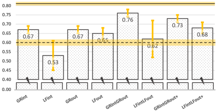
(a) TestRc

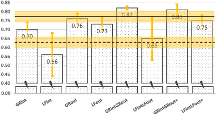
(b) TestRj

Figure 2: F1-Score of adversarial adaptation methods compared to upper bound and lower bound methods.

3.2 Experimental Protocols

Our localization model, $M$ has the encoder-decoder architecture from [20]. We also adopted the same input features which are short-time Fourier transform (STFT) detailed in [20]. These are first processed in individual encoders for each microphone array, merged and then decoded together. Weights between array-encoders are shared. Discrimination is conducted on the merged encoded features for int-dist, and localization heatmaps for out-dist. The discriminator architecture for int-dist consists of $4$ dense layers while out-dist is composed of $4$ convolutional layers followed by $3$ dense layers. A ReLu activation function is used for each layer, except the last one which has a sigmoid activation. ADAM optimizer is used with an initial learning rate of $10^{-4},\beta=(0.5,0.999)$ and a batch size of $256$ samples.

To evaluate, we used precision, recall and F1-score as described in [20]. The source coordinates are extracted from the output heatmap as predicted keypoints. These are matched with the groundtruth keypoints with a resolution threshold of $1$m. Based on the matches, we count true positives (TP), false positives (FP) and false negatives (FN), which are used to get the F1-score. Root mean square error (RMSE) of the matches is provided as an additional indicator of the quality.

Each method is trained for $200$ epochs and this model is tested on both TestRc and TestRj. For all domain adaptation methods, we also present results with model selection (from the $200$ epochs) using the best F1-score on ValidR. Although this is a common measure against overfitting, it can only be done by using some real labeled data so we separate this result into the Sel. column.

We report the mean and standard deviation of 5 independently trained models with different random seeds.

• Lower bound method S is a supervised method trained on labeled synthetic data (TrainS). It represents the minimum performance without any knowledge of the target domain.

• Upper bound method R is a supervised method trained on labeled real-world data (TrainR). It is an approximation of the maximum performance [23], when a lot of effort is spent to label real-world data which we would like to avoid in practice.

• Others refers to methods modifying the training data. Method R&S uses data augmentation by using TrainR and TrainS, both with labels, to train $M$. It sacrifices data quality by mixing domains, but has the same data quantity used in the adversarial methods. The main burden is that it requires labels for the real-world data. Method S+ uses domain randomization [30] by using TrainS+ instead of TrainS in method S.

• Adversarial Adaptation methods are the variations of unsupervised domain adaptation using adversarial learning that we described. These are trained on TrainS with labels and TrainR without labels. The studied methods are: G_rint, L_fint, G_rout, L_fout, and ensemble methods G_rintG_rout and L_fintL_fout. G_r and L_f, refer to gradient reversal and label flipping respectively. int and out are short for the discrimination level int-dist and out-dist. We also considered G_rintG_rout+ and L_fintL_fout+ which used TrainS+ instead of TrainS.

3.3 Results and Discussion

Table 1: Domain Adaptation Results on Additional Metrics

		TestRc (classical & funk)
Method		RMSE $\downarrow$	Precision $\uparrow$	Recall $\uparrow$
Low B.	S	.51$\pm$.01	.80$\pm$.03	.48$\pm$.03
Up B.	R	.34$\pm$.01	.95$\pm$.03	.71$\pm$.03
Others	R&S	.33$\pm$.02	.96$\pm$.03	.71$\pm$.04
	S+	.44$\pm$.00	.84$\pm$.01	.57$\pm$.01
Adv. Adap.	GRint	.48$\pm$.03	.81$\pm$.05	.57$\pm$.04
	LFint	.50$\pm$.03	.71$\pm$.06	.44$\pm$.09
	GRout	.51$\pm$.02	.68$\pm$.02	.67$\pm$.02
	LFout	.51$\pm$.02	.64$\pm$.04	.67$\pm$.02
	GRintGRout	.47$\pm$.05	.82$\pm$.05	.72$\pm$.03
	LFintLFout	.53$\pm$.03	.65$\pm$.10	.60$\pm$.09
	GRintGRout+	.46$\pm$.02	.76$\pm$.07	.71$\pm$.05
	LFintLFout+	.50$\pm$.02	.72$\pm$.09	.65$\pm$.02

Results for the 200^th epoch of training; Low B., Up B. and Adv. Adap. refer to

lower bound, upper bound and adversarial adaptation respectively;

$\uparrow$/$\downarrow$ represent the higher/lower is better respectively.

Insights about the localization performance across all studied methods for TestRc can be found in Fig. 2a and Table 1. For method S, which is our lower bound baseline, there are not many detections (low recall) but they are mostly correct (relatively high precision). However, for these correct predictions, the RMSE is relatively high which indicates that the localization quality is low. In comparison, method R which uses labeled real-world data, yields significantly better performance across all metrics compared to method S. In theory [23], our domain adaptation methods should have results within this range. Method R&S marginally improves performance compared to method R on TestRc. Method S+ shows a slight improvement over S but is still far from method R and R&S. Most domain adaptation methods, especially the ensemble discrimination methods, improve the performance compared to the lower bound method S. In particular, the improvement of the recall for some of the proposed methods compared to S is significant and leads to higher F1-score as shown in Fig. 2a.

Fig. 2b shows F1-score of TestRj. The results of domain adaptation seems to be even better on TestRj even though the model is trained on classifical and funk excerpts. We speculate that this is due to TrainS being more similar to TestRj in terms of spectral features. This explains why lower bound S is slightly higher for TestRj while upper bound R is slightly lower.

One of our proposed ensemble discrimination methods, G_rintG_rout, lead to the best results across all test sets. From Table 1 we can see that methods with int-dist lead to a higher precision and a lower RMSE while out-dist mainly increases recall. We think that aligning the intermediate features improves the existing detections while out-dist encourages more detections but at a higher risk of false positives. This interpretation is further supported by our ensembling results. Whereas, int-dist and out-dist can independently lead to a similar F1-score, combining them gives the best results. The best emsemble method is able to perform almost as good as method R while not having any label for the real data. Our attempt to further improve the ensembling results with randomization (using TrainS+ instead of TrainS) did not show any clear benefit.

Table 2: Comparison of F1-Score with/without Model Selection.

		F1-Score $\uparrow$
Test Data		TestRc (classical&funk)			TestRj (jazz)
Stopping Epoch		200th	Sel.		200th	Sel.
Adv. Adap.	GRint	.67$\pm$.02	.71$\pm$.02		.70$\pm$.04	.77$\pm$.03
	LFint	.53$\pm$.08	.64$\pm$.03		.56$\pm$.12	.69$\pm$.03
	GRout	.67$\pm$.02	.72$\pm$.03		.76$\pm$.03	.79$\pm$.03
	LFout	.65$\pm$.03	.73$\pm$.02		.73$\pm$.04	.80$\pm$.01
	GRintGRout	.76$\pm$.02	.79$\pm$.01		.82$\pm$.01	.84$\pm$.01
	LFintLFout	.62$\pm$.10	.74$\pm$.03		.65$\pm$.12	.81$\pm$.03
	GRintGRout+	.73$\pm$.02	.78$\pm$.02		.81$\pm$.03	.85$\pm$.03
	LFintLFout+	.68$\pm$.03	.79$\pm$.02		.75$\pm$.03	.84$\pm$.01

Adv. Adap., and Sel. is short for adversarial adaptation, and model selection;

$\uparrow$ represent the higher is better.

Up to this point, the domain adaptation methods that have been presented did not use any label for the real data. As we can see in Table 2, model selection can further improve performance across all methods at the price of requiring a small labeled real-world dataset for validation (ValidR). Methods based on G_r and L_f generally provide improved F1-score compared to S except for L_fint. Methods based on L_f have lower performance and higher variance when using the last epoch model. Model selection mitigates both issues but G_r is still marginally better.

Finally, we note that although most of our results are contrary to the results in [19], adversarial methods are notoriously difficult to train [33]. The high variance of L_f in our experimental results further supports this.

4 Conclusion

In this paper we studied adversarial domain adaptation methods from synthetic to real-world data for deep learning based multiple sound source 2D localization. These methods, using labeled synthetic data and unlabeled real-world data, yield a significant improvement compared to solely training on synthetic data at a much lower cost than training on labeled real-world data. Moreover, extensive experiments showed that our novel ensemble discrimination method led to the best results, improving over single discrimination methods by a clear margin.

References

- [1] M. Vacher, F. Portet, A. Fleury, and N. Noury, “Development of audio sensing technology for ambient assisted living: Applications and challenges,” in International Journal of E-Health and Medical Communications (IJEHMC), 2011.
- [2] P. Jeyasingh and M. Mohamed Ismail, “Real-time multi source speech enhancement based on sound source separation using microphone array,” in 2018 Conference on Emerging Devices and Smart Systems (ICEDSS), 2018, pp. 183–187.
- [3] S. Argentieri, P. Danes, and P. Souères, “A survey on sound source localization in robotics: From binaural to array processing methods,” Computer Speech & Language, vol. 34, no. 1, pp. 87–112, 2015.
- [4] M. Cobos, F. Antonacci, A. Alexandridis, A. Mouchtaris, and B. Le, “A survey of sound source localization methods in wireless acoustic sensor networks,” Wireless Communications and Mobile Computing, 2017.
- [5] L. Netsch and J. Stachurski, “Robust low-resource sound localization in correlated noise,” in INTERSPEECH 2014, 15th Annual Conference of the International Speech Communication Association, Singapore, September 14-18, 2014. ISCA, 2014, pp. 2218–2222.
- [6] W.-K. Ma, B.-N. Vo, S. S. Singh, and A. Baddeley, “Tracking an unknown time-varying number of speakers using tdoa measurements: a random finite set approach,” IEEE Transactions on Signal Processing, vol. 54, no. 9, pp. 3291–3304, Sep. 2006.
- [7] A. Alexandridis and A. Mouchtaris, “Multiple sound source location estimation in wireless acoustic sensor networks using doa estimates: The data-association problem,” IEEE/ACM Trans. Audio, Speech and Lang. Proc., vol. 26, no. 2, pp. 342–356, Feb. 2018.
- [8] Y. Guo, X. Wang, C. Wu, Q. Fu, N. Ma, and G. Brown, “A robust dual-microphone speech source localization algorithm for reverberant environments,” in Interspeech. ISCA, September 2016.
- [9] J. Salamon and J. Bello, “Deep convolutional neural networks and data augmentation for environmental sound classification,” IEEE Signal Processing Letters, vol. 24, no. 3, pp. 279–283, 3 2017.
- [10] T. Inoue, P. Vinayavekhin, S. Wang, D. Wood, N. Greco, and R. Tachibana, “Domestic activities classification based on CNN using shuffling and mixing data augmentation,” DCASE2018 Challenge, Tech. Rep., September 2018.
- [11] P. Pertilä and E. Cakir, “Robust direction estimation with convolutional neural networks based steered response power,” in 2017 IEEE International Conference on Acoustics, Speech and Signal Processing (ICASSP), March 2017, pp. 6125–6129.
- [12] S. Adavanne, A. Politis, and T. Virtanen, “Direction of arrival estimation for multiple sound sources using convolutional recurrent neural network,” in 26th European Signal Processing Conference (EUSIPCO), Sep. 2018, pp. 1462–1466.
- [13] W. He, P. Motlicek, and J.-M. Odobez, “Joint localization and classification of multiple sound sources using a multi-task neural network,” in Proc. Interspeech, 2018, pp. 312–316.
- [14] W. He, P. Motlicek, and J. Odobez, “Deep neural networks for multiple speaker detection and localization,” in IEEE International Conference on Robotics and Automation (ICRA), May 2018, pp. 74–79.
- [15] R. Takeda and K. Komatani, “Sound source localization based on deep neural networks with directional activate function exploiting phase information,” in IEEE International Conference on Acoustics, Speech and Signal Processing (ICASSP), March 2016, pp. 405–409.
- [16] J. Vera-Diaz, D. Pizarro, and J. Macias-Guarasa, “Towards end-to-end acoustic localization using deep learning: From audio signals to source position coordinates,” Sensors, vol. 18, no. 10, p. 3418, Oct 2018.
- [17] H. Pujol, E. Bavu, and A. Garcia, “Source localization in reverberant rooms using deep learning and microphone arrays,” in 23rd International Congress on Acoustics (ICA 2019 Aachen), 2019.
- [18] N. Ma, T. May, and G. J. Brown, “Exploiting deep neural networks and head movements for robust binaural localization of multiple sources in reverberant environments,” IEEE/ACM Transactions on Audio, Speech, and Language Processing, vol. 25, no. 12, pp. 2444–2453, Dec 2017.
- [19] W. He, P. Motlicek, and J. Odobez, “Adaptation of multiple sound source localization neural networks with weak supervision and domain-adversarial training,” in IEEE International Conference on Acoustics, Speech and Signal Processing (ICASSP), May 2019, pp. 770–774.
- [20] G. Le Moing, P. Vinayavekhin, T. Inoue, J. Vongkulbhisal, A. Munawar, R. Tachibana, and D. J. Agravante, “Learning multiple sound source 2d localization,” in IEEE 21st International Workshop on Multimedia Signal Processing (MMSP), 2019.
- [21] N. Yalta, K. Nakadai, and T. Ogata, “Sound source localization using deep learning models,” Journal of Robotics and Mechatronics, vol. 29, no. 1, pp. 37–48, 2017.
- [22] D. D. Carlo, A. Deleforge, and N.Bertin, “Mirage: 2d source localization using microphone pair augmentation with echoes,” in ICASSP 2019 - 2019 IEEE International Conference on Acoustics, Speech and Signal Processing (ICASSP), 2019, pp. 775–779.
- [23] S. Ben-David, J. Blitzer, K. Crammer, A. Kulesza, F. Pereira, and J. Vaughan, “A theory of learning from different domains,” Machine Learning, vol. 79, pp. 151–175, 2010.
- [24] R. Takeda and K. Komatani, “Unsupervised adaptation of deep neural networks for sound source localization using entropy minimization,” in IEEE International Conference on Acoustics, Speech and Signal Processing (ICASSP), March 2017, pp. 2217–2221.
- [25] R. Takeda, Y. Kudo, K. Takashima, Y. Kitamura, and K. Komatani, “Unsupervised adaptation of neural networks for discriminative sound source localization with eliminative constraint,” in IEEE International Conference on Acoustics, Speech and Signal Processing (ICASSP), April 2018, pp. 3514–3518.
- [26] Y. Ganin, E. Ustinova, H. Ajakan, P. Germain, H. Larochelle, F. Laviolette, M. March, and V. Lempitsky, “Domain-adversarial training of neural networks,” Journal of Machine Learning Research, vol. 17, no. 59, pp. 1–35, 2016.
- [27] T.-H. Vu, H. Jain, M. Bucher, M. Cord, and P. Pérez, “Advent: Adversarial entropy minimization for domain adaptation in semantic segmentation,” in CVPR, 2019.
- [28] W. Wei, H. Zhu, E. Benetos, and Y. Wang, “A-crnn: A domain adaptation model for sound event detection,” in ICASSP 2020 - 2020 IEEE International Conference on Acoustics, Speech and Signal Processing (ICASSP), 2020, pp. 276–280.
- [29] S. Gharib, K. Drossos, E. Cakir, D. Serdyuk, and T. Virtanen, “Unsupervised adversarial domain adaptation for acoustic scene classification,” in Proceedings of the Detection and Classification of Acoustic Scenes and Events 2018 Workshop (DCASE2018), November 2018, pp. 138–142.
- [30] J. Tobin, R. Fong, A. Ray, J. Schneider, W. Zaremba, and P. Abbeel, “Domain randomization for transferring deep neural networks from simulation to the real world,” IEEE/RSJ International Conference on Intelligent Robots and Systems (IROS), pp. 23–30, 2017.
- [31] I. Goodfellow, J. Pouget-Abadie, M. Mirza, B. Xu, D. Warde-Farley, S. Ozair, A. Courville, and Y. Bengio, “Generative adversarial nets,” in Advances in Neural Information Processing Systems 27, 2014, pp. 2672–2680.
- [32] R. Scheibler, E. Bezzam, and I. Dokmanic, “Pyroomacoustics: A python package for audio room simulation and array processing algorithms,” in IEEE International Conference on Acoustics, Speech, and Signal Processing (ICASSP), 9 2018.
- [33] M. Lucic, K. Kurach, M. Michalski, S. Gelly, and O. Bousquet, “Are gans created equal? a large-scale study,” in Advances in Neural Information Processing Systems 31, 2018, pp. 700–709.