Domain walls and CP violation with left right supersymmetry :

implications for leptogenesis and electron EDM

Piyali Banerjee and Urjit A. Yajnik

Department of Physics, Indian Institute of Technology Bombay, Mumbai 400076, India

Abstract

Low scale leptogenesis scenarios are difficult to verify due to our inability to relate the parameters involved in the early universe processes with the low energy or collider observables. Here we show that one can in principle relate the parameters giving rise to the transient $CP$ violating phase involved in leptogenesis with those that can be deduced from the observation of electric dipole moment (EDM) of the electron. We work out the details of this in the context of the left right symmetric supersymmetric model (LRSUSY) which provides a strong connection between such parameters. In particular, we show that baryon asymmetry requirements imply the scale $M_{B-L}$ of $U(1)_{B-L}$ symmetry breaking to be larger than $10^{4.5}~{}\mathrm{GeV}$. Moreover the scale $M_{R}$ of $\mathrm{SU}(2)_{R}$ symmetry breaking is tightly constrained to lie in a narrow band significantly below $M_{B-L}^{2}/M_{EW}$. These are the most stringent constraints on the parameter space of LRSUSY model being considered.

PACS Numbers:

I Introduction

One of the three necessary Sakharov conditions for dynamical generation of baryon asymmetry of the universe is CP violation Sakharov . The Standard Model (SM) of particle physics has the ingredients to satisfy all the three Sakharov conditions and could, in principle, generate some baryon asymmetryKuzmin . However the requirement of a first order Electroweak Phase Transition (EWPT) requires the mass of the Higgs to remain less than about 80 GeV Kajantie1 ; Kajantie2 ; Csikor which is far below the mass of the recently discovered SM Higgs boson Exptmass1 ; Exptmass2 . Furthermore the CP violation in the CKM matrix of SM is too small to produce a reasonably large baryon asymmetry Gavela .

The left right symmetric model of Mohapatra and Senjanović MohapatraLR (LRSM) is a minimal extension of the Standard Model based on the gauge group $\mathrm{SU}(3)_{c}\times\mathrm{SU}(2)_{L}\times\mathrm{SU}(2)_{R}\times\mathrm{U}(1)_{B-L}$ augmented with the discrete $Z_{2}$ left-right symmetry. The usual $\mathrm{SU}(2)_{L}$ Higgs doublet of SM is extended to a $\mathrm{SU}(2)_{L}\times\mathrm{SU}(2)_{R}$ bidoublet. The model naturally accommodates the parity violation of SM as a result of spontaneous symmetry breaking of $\mathrm{SU}(2)_{R}\times\mathrm{U}(1)_{B-L}$ and also elegantly explains small neutrino masses via the seesaw mechanism. Both goals are achieved by adding new heavy Higgs $\mathrm{SU}(2)$ triplets in the theory.

The supersymmetric extension of LRSM, which we call the Simplified Left Right Symmetric Supersymmetric Standard Model (SLRSUSY), marries the desirable features of both LRSM and supersymmetry. However it suffers from the drawback that spontaneous parity violation cannot take place without violating R-parity also Kuchimanchi . To remedy this, one can take the supersymmetry breaking scale $M_{S}$ to be larger than the $\mathrm{SU}(2)_{R}\times\mathrm{U}(1)_{B-L}$ breaking scale $M_{B-L}$ but that would lose out on several desirable features of supersymmetry. Alternatively, one can introduce additional heavy Higgs $\mathrm{SU}(2)$ triplets with appropriate gauge group charges. This was done in the two papers Aulakh:1997ba ; Aulakh:1997fq , which we shall call the Left Right Symmetric Supersymmetric Standard Model (LRSUSY). The LRSUSY model contains two distinct high mass scales, $M_{R}$ the scale of $\mathrm{SU}(2)_{R}$ symmetry breaking, and $M_{B-L}$ the scale of $U(1)_{B-L}$ symmetry breaking satisfying $M_{R}\gg M_{B-L}$, an intermediate SUSY breaking scale $M_{S}$ and a low mass scale $M_{H}$ where the bidoublet Higgs get vevs. Thus, the LRSUSY model has several desirable features not possessed by SLRSUSY like spontaneous parity violation without R-parity violation, low scale supersymmetry with exact R-parity and existence of a stable lightest supersymmetric particle.

Breaking of the $Z_{2}$ discrete symmetry of left-right symmetric models in the early universe ensures the occurrence of domain walls, but also begs for the $Z_{2}$ symmetry to be not exact to avoid conflict with the observed homogeneous universe. However an approximate $Z_{2}$ is adequate to generate the domain walls which are a robust topological prediction independent of details of parameters, and can play the same role as the phase transition bubble walls for the purpose of leptogenesis.

In the context of non-supersymmetric LRSM, fate of the $CP$ violating phase was studied in ClineYajnik for the purpose of explaining leptogenesis. It was shown that a spatially varying CP violating phase occurs inside the domain walls separating the left handed and right handed domains. They showed that in order to explain the observed baryon asymmetry of the universe, the Yukawa coupling of the right handed neutrino to the $\mathrm{SU}(2)$-triplet Higgs must be larger than $10^{-2}$. They also obtained some heuristic constraints on the mass of the left handed neutrinos or alternatively, the temperature scale of LR symmetry breaking. Since the LRSUSY model has additional Higgs bosons as well as additional CP violating phases, it may be able to generate the necessary conditions for successful baryogenesis in the early universe. The first step in this direction was taken in Anjishnu by showing the possibility of having a spatially varying CP violating phase in the domain walls in the context of LRSUSY. However they did not provide any quantitative estimates and left open the question of whether LRSUSY is actually capable of generating the baryon asymmetry of the universe.

The core idea of such proposals is that the spatially varying phase implies a spatially varying complex mass for left handed neutrinos inside the wall. Studying the diffusion equation for lepton number density with spatially varying complex mass results in the preferential transmission of left handed neutrinos across a slowly moving thick domain wall. The moving wall encroaches upon the energetically disfavoured right handed domain. We solve the diffusion equation numerically for various wall speeds and thicknesses, obtaining excesses of almost massless left handed neutrinos inside the left handed domain. After the wall disappears, electroweak sphaelerons convert a part of the neutrino excess to baryon excess. We calculate the amount of baryon excess that survives the washout processes. Requiring the surviving baryon excess to be not much above the experimental limit of around $6\times 10^{-10}$ for the baryon asymmetry to entropy ratio Canetti allows us to constrain the $(M_{R},M_{B-L})$ parameter space of LRSUSY.

A smoking gun signature of CP violation in a theory is the presence of a non-zero EDM of the electron and neutron. The Standard Model predicts a non-zero electron EDM at the three loop level but the effect is estimated to be very small, around $1.9\times 10^{-39}~{}\mathrm{e~{}cm}$ YamaguchiYamanaka . This is way below the current experimental upper bound of $1.1\times 10^{-29}~{}\mathrm{e~{}cm}$ obtained by the ACME II experiment ACME2 . Left right symmetric theories contain many additional sources of CP violation as compared to the Standard Model, and so predict larger electron and neutron EDMs. Thus the experimental bound on EDMs serve to constrain the parameters of these theories. Electron and neutron EDMs in the non-supersymmetric LRSM have been studied in several earlier works e.g. Nieves ; Xu , obtaining lower bounds on the scale $M_{B-L}$ of $\mathrm{SU}(2)_{R}\times U(1)_{B-L}$ symmetry breaking and on the mass $M_{H^{\prime}}$ of the heavier scalar Higgs in the two Higgs doublets arising from breaking of left right symmetry in the bidoublet Higgs of LRSM. Electron and neutron EDMs have been studied in the SLRSUSY model by FrankE ; FrankN , obtaining bounds on the masses of certain superpartners and some other parameters of SLRSUSY.

The LRSUSY modelAulakh:1997fq contains essentially only one major unknown, the $M_{R}$ scale and a trilinear Higgs coupling parameter $\alpha$ that is used to ensure that only two out of four SM type Higgs doublets arising after $\mathrm{SU}(2)_{R}\times\mathrm{U}(1)_{B-L}$ symmetry breaking remain lighter, with a relative phase between their vacuum expectation values. In this paper we study the CP violating phase of the bidoublet fields in LRSUSY by setting up the domain wall solutions. The parameters relevant for the domain wall solutions are understood to involve the high temperature corrections needed in the early Universe, at the temperature $T_{B-L}\sim M_{B-L}$. We separately investigate the contribution of the lighter two mass eigenstates of the bidoublets to the electron EDM at zero temperature, which differ only by the $T_{B-L}$ corrections. We compute the contribution of this low energy phase to the EDM at one loop and two loop levels as a function of $\alpha$. The two loop computation follows along the lines of the seminal work of Barr and Zee BarrZee on the electron EDM in multi Higgs doublet models. A similar calculation of electron EDM arising as a residual effect of domain wall collapse in two Higgs doublet models was done in Chen . It turns out that successful leptogenesis in LRSUSY requires $\alpha\gtrsim 0.1$. Combining this with the requirement that the EDM obtained be less than the experimental limit of $1.1\times 10^{-29}~{}\mbox{e cm}$, we get an allowed region in the $(M_{B-L},M_{R})$-parameter space of LRSUSY.

It turns out that the limit on the parameter space arising from baryon asymmetry is more stringent than the limit from electron EDM. Further requiring that the observed baryon asymmetry be explained to within an order of magnitude by LRSUSY puts stringent constraints on the $(M_{B-L},M_{R})$-parameter space of LRSUSY. In particular $M_{B-L}<10^{4.5}~{}\mathrm{GeV}$ is ruled out. These are the most stringent constraints on the parameter space of LRSUSY by far.

II The LRSUSY model revisited

The gauge group of LRSUSY is the left-right symmetric group $\mathrm{SU}(3)_{c}\times\mathrm{SU}(2)_{L}\times\mathrm{SU}(2)_{R}\times\mathrm{U}(1)_{B-L}$. The Higgs sector consists of two Higgs bidoublets $\Phi_{1}$ and $\Phi_{2}$, three left handed Higgs triplets $\Delta$, $\bar{\Delta}$ and $\Omega$, and three right handed Higgs triplets $\Delta_{c}$, $\bar{\Delta}_{c}$ and $\Omega_{c}$. Following Kuchimanchi-Mohapatra Kuchimanchi , the gauge group charges are

$$\begin{array}[]{c c l c c l c c l}\Phi_{1}&=&(1,2,2^{*},0),&\Phi_{2}&=&(1,2,2^{*},0),&\\ \Omega&=&(1,3,1,0),&\Delta&=&(1,3,1,2),&\bar{\Delta}&=&(1,3,1,-2),\\ \Omega_{c}&=&(1,1,3^{*},0),&\Delta_{c}&=&(1,1,3^{*},-2),&\bar{\Delta}_{c}&=&(1,1,3^{*},2).\end{array}$$ (1)

In other words, the group action is given by

$$\{\Phi_{1},\Phi_{2}\}\rightarrow U_{L}\{\Phi_{1},\Phi_{2}\}U_{R}^{\dagger},~{}~{}~{}\{\Delta,\bar{\Delta},\Omega\}\rightarrow U_{L}\{\Delta,\bar{\Delta},\Omega\}U_{L}^{\dagger},~{}~{}~{}\{\Delta_{c},\bar{\Delta}_{c},\Omega_{c}\}\rightarrow U_{R}^{*}\{\Delta_{c},\bar{\Delta}_{c},\Omega_{c}\}U_{R}^{T}.$$ (2)

The electric charge is given by $Q=T_{3L}+T_{3R}+\frac{B-L}{2}.$ From Aulakh et al. Aulakh:1997fq the Higgs part of the superpotential is given by

$$\begin{array}[]{rcl}W&=&m_{\Delta}(\mathrm{Tr}\,\Delta\bar{\Delta}+\Delta_{c}\bar{\Delta}_{c})+\frac{m_{\Omega}}{2}(\mathrm{Tr}\,\Omega^{2}+\mathrm{Tr}\,\Omega_{c}^{2})+\mu_{ij}\mathrm{Tr}\,\tau_{2}\Phi_{i}^{T}\tau_{2}\Phi_{j}\\ &&{}+a(\mathrm{Tr}\,\Delta\Omega\bar{\Delta}+\mathrm{Tr}\,\Delta_{c}\Omega_{c}\bar{\Delta}_{c})+\alpha_{ij}(\mathrm{Tr}\,\Omega\Phi_{i}\tau_{2}\Phi_{j}^{T}\tau_{2}+\mathrm{Tr}\,\Omega_{c}\Phi_{i}^{T}\tau_{2}\Phi_{j}\tau_{2}),\end{array}$$ (3)

where $\alpha_{ij}$, $\mu_{ij}$ are complex numbers satisfying $\mu_{12}=\mu_{21}$, $\alpha_{ij}=-\alpha_{ji}$. Define $\alpha=\alpha_{12}$. Then $\alpha_{21}=-\alpha$ and $\alpha_{11}=\alpha_{22}=0$.

The charge zero condition forces the vevs of the Higgs fields to be

$$\begin{array}[]{c c l c c l c c l}\langle\Phi_{1}\rangle&=&\left(\begin{array}[]{c c}k_{1}&0\\ 0&k_{1}^{\prime}\end{array}\right),&\langle\Phi_{2}\rangle&=&\left(\begin{array}[]{c c}k_{2}&0\\ 0&k_{2}^{\prime}\end{array}\right),&\\ \langle\Omega\rangle&=&\left(\begin{array}[]{c c}\omega&0\\ 0&-\omega\end{array}\right),&\langle\Delta\rangle&=&\left(\begin{array}[]{c c}0&0\\ d&0\end{array}\right),&\langle\bar{\Delta}\rangle&=&\left(\begin{array}[]{c c}0&\bar{d}\\ 0&0\end{array}\right),\\ \langle\Omega_{c}\rangle&=&\left(\begin{array}[]{c c}\omega_{c}&0\\ 0&-\omega_{c}\end{array}\right),&\langle\Delta_{c}\rangle&=&\left(\begin{array}[]{c c}0&0\\ d_{c}&0\end{array}\right),&\langle\bar{\Delta}_{c}\rangle&=&\left(\begin{array}[]{c c}0&\bar{d}_{c}\\ 0&0\end{array}\right),\end{array}$$ (4)

where the quantities above are in general complex numbers.

The D-terms are given by (where $m=1,2,3$ refer to the three generators of $\mathrm{SU}(2)$) Kuchimanchi

$$\begin{array}[]{rcl}D_{L,m}&=&\mathrm{Tr}\,(2\Omega^{\dagger}\tau_{m}\Omega+2\Delta^{\dagger}\tau_{m}\Delta+2\bar{\Delta}^{\dagger}\tau_{m}\bar{\Delta}+\Phi_{1}^{\dagger}\tau_{m}\Phi_{1}+\Phi_{2}^{\dagger}\tau_{m}\Phi_{2})\\ D_{R,m}&=&\mathrm{Tr}\,(2\Omega_{c}^{\dagger}\tau_{m}\Omega_{c}+2\Delta_{c}^{\dagger}\tau_{m}\Delta_{c}+2\bar{\Delta}_{c}^{\dagger}\tau_{m}\bar{\Delta}_{c}+\Phi_{1}\tau_{m}^{T}\Phi_{1}^{\dagger}+\Phi_{2}\tau_{m}^{T}\Phi_{2}^{\dagger})\\ D_{B-L}&=&\mathrm{Tr}\,(2\Delta^{\dagger}\Delta-2\bar{\Delta}^{\dagger}\bar{\Delta}-2\Delta_{c}^{\dagger}\Delta_{c}+2\bar{\Delta}_{c}^{\dagger}\bar{\Delta}_{c}).\end{array}$$ (5)

After substituting the vevs into the D-term expressions we get

$$\begin{array}[]{rcl}\langle D_{B-L}\rangle&=&2(|d|^{2}-|\bar{d}|^{2}-|d_{c}|^{2}+|\bar{d}_{c}|^{2}),\\ \langle D_{L,1}\rangle&=&\langle D_{L,2}\rangle=\langle D_{R,1}\rangle=\langle D_{R,2}\rangle=0,\\ \langle D_{L,3}\rangle&=&2(-|d|^{2}+|\bar{d}|^{2})+|k_{1}|^{2}-|k_{1}^{\prime}|^{2}+|k_{2}|^{2}-|k_{2}^{\prime}|^{2},\\ \langle D_{R,3}\rangle&=&2(-|d_{c}|^{2}+|\bar{d}_{c}|^{2})+|k_{1}|^{2}-|k_{1}^{\prime}|^{2}+|k_{2}|^{2}-|k_{2}^{\prime}|^{2}.\end{array}$$ (6)

Taking $|d|=|\bar{d}|$ and $|d_{c}|=|\bar{d}_{c}|$ ensures the vanishing of $D_{B-L}$-term always. We can use the $B-L$ gauge invariance to ensure that $d$, $\bar{d}$ have the same complex phase. Subsequently using $\mathrm{SU}(2)_{L}$ invariance, we can ensure that $d=\bar{d}$ and real positive.

Extending Aulakh et al, we see that the resulting F-terms are:

$$\begin{array}[]{rcl}F_{\bar{\Delta}}&=&m_{\Delta}\Delta+a(\Delta\Omega-\frac{\mathrm{Tr}\,\Delta\Omega}{2}),\\ F_{\Delta}&=&m_{\Delta}\bar{\Delta}+a(\Omega\bar{\Delta}-\frac{\mathrm{Tr}\,\Omega\bar{\Delta}}{2}),\\ F_{\Omega}&=&m_{\Omega}\Omega+a(\bar{\Delta}\Delta-\frac{\mathrm{Tr}\,\bar{\Delta}\Delta}{2})+\alpha(\Phi_{1}\tau_{2}\Phi_{2}^{T}\tau_{2}-\Phi_{2}\tau_{2}\Phi_{1}^{T}\tau_{2}),\\ F_{\bar{\Delta_{c}}}&=&m_{\Delta}\Delta_{c}+a(\Delta_{c}\Omega_{c}-\frac{\mathrm{Tr}\,\Delta_{c}\Omega_{c}}{2}),\\ F_{\Delta_{c}}&=&m_{\Delta}\bar{\Delta_{c}}+a(\Omega_{c}\bar{\Delta_{c}}-\frac{\mathrm{Tr}\,\Omega_{c}\bar{\Delta_{c}}}{2}),\\ F_{\Omega_{c}}&=&m_{\Omega}\Omega_{c}+a(\bar{\Delta_{c}}\Delta_{c}-\frac{\mathrm{Tr}\,\bar{\Delta_{c}}\Delta_{c}}{2})+\alpha(\Phi_{1}^{T}\tau_{2}\Phi_{2}\tau_{2}-\Phi_{2}^{T}\tau_{2}\Phi_{1}\tau_{2}),\\ F_{\Phi_{1}}&=&2\mu_{11}\tau_{2}\Phi_{1}^{T}\tau_{2}+2\mu_{12}\tau_{2}\Phi_{2}^{T}\tau_{2}+\alpha(\tau_{2}\Phi_{2}^{T}\tau_{2}\Omega-\tau_{2}\Phi_{2}^{T}\Omega^{T}\tau_{2}+\tau_{2}\Omega_{c}\Phi_{2}^{T}\tau_{2}-\Omega_{c}^{T}\tau_{2}\Phi_{2}^{T}\tau_{2}),\\ F_{\Phi_{2}}&=&2\mu_{12}\tau_{2}\Phi_{1}^{T}\tau_{2}+2\mu_{22}\tau_{2}\Phi_{2}^{T}\tau_{2}-\alpha(\tau_{2}\Phi_{1}^{T}\tau_{2}\Omega-\tau_{2}\Phi_{1}^{T}\Omega^{T}\tau_{2}+\tau_{2}\Omega_{c}\Phi_{1}^{T}\tau_{2}-\Omega_{c}^{T}\tau_{2}\Phi_{1}^{T}\tau_{2}).\end{array}$$ (7)

After substituting the vevs, the expressions for the F-terms become

$$\begin{array}[]{rcl}\langle F_{\bar{\Delta}}\rangle&=&\left(\begin{array}[]{c c}0&0\\ d(m_{\Delta}+a\omega)&0\end{array}\right),\\ \langle F_{\Delta}\rangle&=&\left(\begin{array}[]{c c}0&\bar{d}(m_{\Delta}+a\omega)\\ 0&0\end{array}\right),\\ \langle F_{\Omega}\rangle&=&\left(\begin{array}[]{c c}m_{\Omega}\omega+\frac{ad\bar{d}}{2}+\alpha(k_{1}k_{2}^{\prime}-k_{1}^{\prime}k_{2})&0\\ 0&-(m_{\Omega}\omega+\frac{ad\bar{d}}{2}+\alpha(k_{1}k_{2}^{\prime}-k_{1}^{\prime}k_{2}))\end{array}\right),\\ \langle F_{\bar{\Delta}_{c}}\rangle&=&\left(\begin{array}[]{c c}0&d_{c}(m_{\Delta}+a\omega_{c})\\ 0&0\end{array}\right),\\ \langle F_{\Delta_{c}}\rangle&=&\left(\begin{array}[]{c c}0&0\\ \bar{d}_{c}(m_{\Delta}+a\omega_{c})&0\end{array}\right),\\ \langle F_{\Omega_{c}}\rangle&=&\left(\begin{array}[]{c c}m_{\Omega}\omega_{c}+\frac{ad_{c}\bar{d}_{c}}{2}+\alpha(k_{1}k_{2}^{\prime}-k_{1}^{\prime}k_{2})&0\\ 0&-(m_{\Omega}\omega_{c}+\frac{ad_{c}\bar{d}_{c}}{2}+\alpha(k_{1}k_{2}^{\prime}-k_{1}^{\prime}k_{2}))\end{array}\right),\\ \langle F_{\Phi_{1}}\rangle&=&\left(\begin{array}[]{c c}2\mu_{11}k_{1}^{\prime}+2\mu_{12}k_{2}^{\prime}+2\alpha k_{2}^{\prime}(\omega-\omega_{c})&0\\ 0&2\mu_{11}k_{1}+2\mu_{12}k_{2}-2\alpha k_{2}(\omega-\omega_{c})\\ \end{array}\right),\\ \langle F_{\Phi_{2}}\rangle&=&\left(\begin{array}[]{c c}2\mu_{12}k_{1}^{\prime}+2\mu_{22}k_{2}^{\prime}-2\alpha k_{1}^{\prime}(\omega-\omega_{c})&0\\ 0&2\mu_{12}k_{1}+2\mu_{22}k_{2}+2\alpha k_{1}(\omega-\omega_{c})\\ \end{array}\right).\end{array}$$ (8)

We now investigate what vevs ensure flatness conditions for all the F-terms and all the D-terms. For generic values of $\mu_{11}$, $\mu_{12}$ and $\mu_{22}$, the entries of $F_{\Phi_{1}}$ and $F_{\Phi_{2}}$ are linearly independent. Hence flatness of $F_{\Phi_{1}}$ and $F_{\Phi_{2}}$ implies that the vevs of $k_{1}$, $k^{\prime}_{1}$, $k_{2}$, $k^{\prime}_{2}$ are all zero. This automatically makes $D_{L,3}$ and $D_{R,3}$ flat.

Proceeding ahead, we now see that the F-flatness conditions split into two subsets viz. the left handed conditions and right handed conditions. This allows to conclude, as noted first by Aulakh et al., that the complete solution set for F-flatness and D-flatness is obtained by taking $(\omega,d)=(0,0)$ or $(\omega,d)=(\frac{m_{\Delta}}{-a},\frac{\sqrt{2m_{\Omega}m_{\Delta}}}{-a})$, and $(\omega_{c},d_{c})=(0,0)$ or $(\omega_{c},d_{c})=(\frac{m_{\Delta}}{-a},\frac{\sqrt{2m_{\Omega}m_{\Delta}}}{-a})$ and $(k_{1},k^{\prime}_{1},k_{2},k^{\prime}_{2})=(0,0,0,0)$ (note $a<0$). Thus, the complete SUSY preserving solution set has, beside the trivial all zero solution, three non-trivial solutions. Of these, the solution $(\omega,d,\omega_{c},d_{c},k_{1},k_{1}^{\prime},k_{2},k_{2}^{\prime})=(\frac{m_{\Delta}}{-a},\frac{\sqrt{2m_{\Omega}m_{\Delta}}}{-a},\frac{m_{\Delta}}{-a},\frac{\sqrt{2m_{\Omega}m_{\Delta}}}{-a},0,0,0,0)$ is unphysical because it breaks down the gauge symmetry to $\mathrm{SU}(3)_{c}$ even though it preserves SUSY. The other two solutions are indeed physical and can be interpreted as breaking down the left-right symmetric gauge group $\mathrm{SU}(3)_{c}\times\mathrm{SU}(2)_{L}\times\mathrm{SU}(2)_{R}\times U(1)_{B-L}$ into either the left-handed Minimal Supersymmetric Standard Model (MSSM) $\mathrm{SU}(3)_{c}\times\mathrm{SU}(2)_{L}\times U(1)_{Y}$, or into the right-handed MSSM $\mathrm{SU}(3)_{c}\times\mathrm{SU}(2)_{R}\times U(1)_{Y}$.

The expressions for the vevs must be related to the two physical scales in LRSUSY. We need to set

$$M_{R} \cong \frac{m_{\Delta}}{-a}$$ (9)

$$M_{B-L} \cong \frac{\sqrt{2m_{\Omega}m_{\Delta}}}{-a}$$ (10)

in the LH regions and likewise in the RH regions. A solution to the proliferation of mass scales was sought in Aulakh:1997fq by invoking an $R$ symmetry of the superpotential which forbids the terms $\Omega^{2}$ and $\Omega_{c}^{2}$. The $R$ charge values can be set to

$$\Delta,\bar{\Delta},\Delta_{c},\bar{\Delta_{c}},\Phi_{i} \rightarrow 1$$ (11)

$$\Omega \rightarrow 0$$ (12)

$$L,L_{c},Q,Q_{c} \rightarrow \frac{1}{2}$$ (13)

where the $L$, $Q$ etc are matter superfields which are not relevant to this paper. The terms $\Omega^{2}$ and $\Omega_{c}^{2}$ can then be introduced only as soft terms, with the coefficients $m_{\Omega}=m_{\Omega_{c}}$ determined by SUSY breaking scale $\cong M_{EW}$. This leads to an elegant simplification giving rise to the see-saw relation

$$M_{B-L}^{2}\cong M_{R}M_{EW}$$ (14)

From the cosmological viewpoint, the early universe enters an epoch with two types of domains. In the left handed (LH) domains, the right handed vevs take non-zero values and in the right handed (RH) domains, the left handed vevs take non-zero values. The corresponding SUSY preserving vevs are

$$\begin{array}[]{r c l}(\omega,d,\omega_{c},d_{c},k_{1},k_{1}^{\prime},k_{2},k_{2}^{\prime})&=&(0,0,\frac{m_{\Delta}}{-a},\frac{\sqrt{2m_{\Omega}m_{\Delta}}}{-a},0,0,0,0)~{}~{}~{}\mbox{LH domain},\\ (\omega,d,\omega_{c},d_{c},k_{1},k_{1}^{\prime},k_{2},k_{2}^{\prime})&=&(\frac{m_{\Delta}}{-a},\frac{\sqrt{2m_{\Omega}m_{\Delta}}}{-a},0,0,0,0,0,0)~{}~{}~{}\mbox{RH domain}.\end{array}$$ (15)

The formation of the two types of domains also leads to topological domain walls separating them. This is because together with the breaking of the gauge symmetry, a discrete left-right symmetry is also broken. The presence of these walls or energy barriers conflicts with current cosmology. Several earlier works have discussed how such walls may be made to disappear fast enough so as to be consistent with present day observations Mishra . The older study Anjishnu demonstrated the existence of domain walls containing a CP violating phase in LRSUSY with implications to leptogenesis, but only as a proof-of-concept study. In this paper, we extend their ideas greatly and come up with quantitative estimates relating the parameter ranges that can give rise to the required spatially varying CP violating phase within the domain wall with the non-zero phase required for electron EDM in zero temperature translation invariant theory. The next section provides the details.

To the SUSY scalar potential

$$\begin{array}[]{r c l}V_{\mathrm{SUSY}}&=&|F_{\bar{\Delta}}|^{2}+|F_{\Delta}|^{2}+|F_{\bar{\Delta}_{c}}|^{2}+|F_{\Delta_{c}}|^{2}+|F_{\Omega}|^{2}+|F_{\Omega_{c}}|^{2}+|F_{\Phi_{1}}|^{2}+|F_{\Phi_{2}}|^{2}\\ &&{}+\sum_{m=1}^{3}(|D_{L,m}|^{2}+|D_{R,m}|^{2})+|D_{B-L}|^{2},\end{array}$$ (16)

we add the following soft mass terms for the bidoublets

$$\begin{array}[]{r c l}V_{\mathrm{soft}}&=&-\mu_{1}^{2}\mathrm{Tr}\,(\Phi_{1}^{\dagger}\Phi_{1})-\mu_{2}^{2}\mathrm{Tr}\,(\Phi_{2}^{\dagger}\Phi_{2})\\ &&{}-e^{i\beta_{3}}\mu_{3}^{2}\mathrm{Tr}\,(\Phi_{1}^{\dagger}\tau_{2}\Phi_{1}^{*}\tau_{2})-e^{i\beta_{4}}\mu_{4}^{2}\mathrm{Tr}\,(\Phi_{2}^{\dagger}\tau_{2}\Phi_{2}^{*}\tau_{2})-e^{i\beta_{5}}\mu_{5}^{2}\mathrm{Tr}\,(\Phi_{1}^{\dagger}\tau_{2}\Phi_{2}^{*}\tau_{2})+\mathrm{h.c.},\end{array}$$ (17)

where $\mu_{i}^{2}>0$ and $\beta_{3}$, $\beta_{4}$, $\beta_{5}$ are explicit CP phases. Substituting the vevs we get $\langle V\rangle=\langle V_{\mathrm{SUSY}}\rangle+\langle V_{\mathrm{soft}}\rangle,$ where

$$\langle V_{\mathrm{SUSY}}\rangle = |\langle F_{\bar{\Delta}}\rangle|^{2}+|\langle F_{\Delta}\rangle|^{2}+|\langle F_{\bar{\Delta}_{c}}\rangle|^{2}+|\langle F_{\Delta_{c}}\rangle|^{2}+|\langle F_{\Omega}\rangle|^{2}+|\langle F_{\Omega_{c}}\rangle|^{2}+|\langle F_{\Phi_{1}}\rangle|^{2}+|\langle F_{\Phi_{2}}\rangle|^{2}$$

$${}+|\langle D_{L,3}\rangle|^{2}+|\langle D_{R,3}\rangle|^{2}+|\langle D_{B-L}\rangle|^{2},$$

and

$$\begin{array}[]{rcl}\langle V_{\mathrm{soft}}\rangle&=&-\mu_{1}^{2}(|k_{1}|^{2}+|k^{\prime}_{1}|^{2})-\mu_{2}^{2}(|k_{2}|^{2}+|k^{\prime}_{2}|^{2})\\ &&{}-4\mu_{3}^{2}\mathrm{Re}(e^{i\beta_{3}}k_{1}^{*}(k^{\prime}_{1})^{*})-4\mu_{4}^{2}\mathrm{Re}(e^{i\beta_{4}}k_{2}^{*}(k^{\prime}_{2})^{*})-2\mu_{5}^{2}\mathrm{Re}(e^{i\beta_{5}}(k_{1}^{*}(k^{\prime}_{2})^{*}+(k^{\prime}_{1})^{*}k_{2}^{*})).\end{array}$$ (18)

We shall take the fine tuning condition $\mu_{12}^{2}\approx\mu_{11}\mu_{22}+\alpha^{2}M_{R}^{2}$ of Aulakh et el. Aulakh:1997fq which ensures that out of the four neutral Higgs scalars that arise from the bidoublets after the breaking of $\mathrm{SU}(2)_{R}\times\mathrm{U}(1)_{B-L}$ symmetry, two of them have masses near zero (the other two end up having mass near $M_{R}$). Our soft masses $\mu_{1},\ldots,\mu_{5}$ are chosen to be around $\alpha^{2}M_{R}$, so that at temperatures below the SUSY breaking scale, the two light Higgs scalars eventually become the Higgs bosons of a two Higgs doublet model (2HDM) satisfying $\mathrm{SU}(3)_{c}\times\mathrm{SU}(2)_{L}\times U(1)_{Y}$ gauge symmetry. At even lower temperatures, the SM Higgs boson arises from the 2HDM.

III Spatially varying Higgs vevs

The SUSY scalar potential and the soft mass terms for the bidoublets receive temperature corrections determined by the scale $M_{B-L}$. The temperature dependence of the squared mass term of a Higgs scalar has been evaluated at the one loop level in earlier works Dolan . For this indicative study we shall take the temperature correction to each mass matrix element to beCline2HDM ; AndersonHall ; RamseyEWBG ,

$$(\Delta m^{2})^{T}\sim O(g^{2}T^{2})$$ (19)

The full temperature dependent mass matrix can be found in Appendix B. Thus, going from temperature $M_{B-L}$ to zero temperature entails the lowering of the mass matrix elements by $O(g^{2}T^{2})$. For the leptogenesis calculations, we work at the high temperature $T=M_{B-L}$ with the mass matrix arising from the SUSY scalar potential and the soft masses described above. These choices for the mass parameters ensure that the mass matrix of the bidoublets has a negative eigenvalue inside the wall whereas all its eigenvalues are positive outside. This in turn means that it is energetically favourable for the bidoublet fields to take non-zero vevs inside the wall while continuing to take zero vevs outside, even though the soft terms have negative squared masses. For the zero temperature electron EDM calculation that we do later, we can work in a four Higgs doublet model Cline2HDM ; Fromme with temperature corrections dropped from the mass matrix of Appendix B.

In this section we shall see that, for a certain choice of soft SUSY breaking mass terms for the bidoublets, it becomes energetically favourable for the bidoublet fields to take non-zero vevs within the wall while continuing to take (almost) zero vevs outside it. Moreover, the generic $O(1)$ phases in the soft mass terms entail a consequence that the bidoublet fields take on spatially varying $CP$ violating phases inside the wall while returning to constant non-zero phases outside the wall.

Let the spatial coordinate giving the distance from the wall, in units of inverse temperature $1/T$, be denoted by $x$. The fields constituting the wall have substantial variation only in a narrow region $\Delta x\sim(L/v)$ where $v$ is a generic scalar vacuum expectation value and $L^{-1}\sim\sqrt{\lambda}$ is derived from a generic quartic coupling $\lambda$ of a renormalisable field theory. The SUSY preserving vev 8-tuples inside the two domains are given by Equation 15. We want a smooth variation of the vev 8-tuple as a function of $x$, going from the LH domain to the RH domain passing through the wall on the way. By the argument in the previous section, this necessarily entails breaking SUSY inside the wall. Thus in order to get the shapes of the $x$-dependent vevs of the Higgs fields, we need to first write down a functional for the energy per unit area of the wall and then minimise the functional via Euler-Lagrange equations.

Let $\dot{f}$ denote the derivative of vev of field $f$ with respect to $x$. Let $r_{1}$, $i_{1}$ be the real and imaginary parts of vev of $k_{1}$, $r_{2},i_{2},\ldots,r^{\prime}_{2},i^{\prime}_{2}$ the real and imaginary parts of the vevs of the respective bidoublet fields. We make the simplifying assumptions that the non-bidoublet Higgs fields are real everywhere. The finite temperature energy per unit area, which is the sum of gradient energies and potential energies of all the fields, plus field dependent temperature corrections can now be taken to be,

$$\begin{array}[]{rcl}H^{T}&=&\int\,dx\,(\frac{1}{2}(\dot{\omega}^{2}+\dot{\omega_{c}}^{2}+\dot{d}^{2}+\dot{\bar{d}}^{2}+\dot{d_{c}}^{2}+\dot{\bar{d}_{c}}^{2}\\ &&~{}~{}~{}~{}~{}~{}~{}~{}~{}~{}~{}+\dot{r_{1}}^{2}+\dot{i_{1}}^{2}+\dot{r^{\prime}_{1}}^{2}+\dot{i^{\prime}_{1}}^{2}+\dot{r_{2}}^{2}+\dot{i_{2}}^{2}+\dot{r^{\prime}_{2}}^{2}+\dot{i^{\prime}_{2}}^{2})\\ &&~{}~{}~{}~{}~{}~{}~{}~{}~{}~{}~{}+\langle V_{\mathrm{SUSY}}\rangle+\langle V^{T}_{\mathrm{soft}}\rangle).\end{array}$$ (20)

Here a superscript $T$ on $H$ and $V_{\mathrm{soft}}$ is a reminder of the temperature dependence. We determine the domain wall solutions such that SUSY is preserved asymptotically by the vevs upto relatively small temperature correction. It is only in the narrow region of the wall where the omega fields become small that the temperature dependent terms and soft terms become more significant. In the equations below, all the vev are meant to be temperature dependent, though for simplicity of notation we drop the superscript $T$.

$$\begin{array}[]{c}\langle\omega(-\infty)\rangle=\langle d(-\infty)\rangle=\langle\bar{d}(-\infty)\rangle=0,\\ \langle\omega_{c}(-\infty)\rangle=M_{R},\langle d_{c}(-\infty)\rangle=\langle\bar{d}_{c}(-\infty)\rangle=M_{B-L},\\ \langle r_{1}(-\infty)\rangle=\langle i_{1}(-\infty)\rangle=\langle r^{\prime}_{1}(-\infty)\rangle=\langle i^{\prime}_{1}(-\infty)\rangle=0,\\ \langle r_{2}(-\infty)\rangle=\langle i_{2}(-\infty)\rangle=\langle r^{\prime}_{2}(-\infty)\rangle=\langle i^{\prime}_{2}(-\infty)\rangle=0\end{array}$$ (21)

in the left domain and

$$\begin{array}[]{c}\langle\omega_{c}(\infty)\rangle=\langle d_{c}(\infty)\rangle=\langle\bar{d}_{c}(\infty)\rangle=0,\\ \langle\omega(-\infty)\rangle=M_{R},\langle d(\infty)\rangle=\langle\bar{d}(\infty)\rangle=M_{B-L},\\ \langle r_{1}(\infty)\rangle=\langle i_{1}(\infty)\rangle=\langle r^{\prime}_{1}(\infty)\rangle=\langle i^{\prime}_{1}(\infty)\rangle=0,\\ \langle r_{2}(\infty)\rangle=\langle i_{2}(\infty)\rangle=\langle r^{\prime}_{2}(\infty)\rangle=\langle i^{\prime}_{2}(\infty)\rangle=0\end{array}$$ (22)

in the right domain.

With all the parameters in place, we can now minimise the energy density per unit area by solving the Euler-Lagrange equations arising from Equation 20. The equations are given explicitly in Appendix A for completeness. In the next section we describe how to solve them numerically in order to obtain the shapes of the spatially varying vevs of the Higgs fields both within and outside the wall. The vevs take the limiting values described in Equations 21, 22 outside the wall.

IV Solving the Euler-Lagrange equations for Higgs vevs

The Euler-Lagrange equations in Appendix A form a coupled system of second order non-linear differential equations satisfying the boundary conditions of Equation 21 in the left domain and Equation 22 in the right domain. Since the derivatives of the vevs are zero in both left and right domains, these equations are not well-suited for numerical solution by shooting methods. Because of the large number of non-linear equations, their numerical solution also faces difficulties under finite element or path deformation Wainwright methods.

Naive attempts to solve the Euler-Lagrange equations as an initial value system also run into problems. This is because if we take the initial conditions at a point in the left domain, the algorithms give us the SUSY flat left domain solution only as that solution minimises the energy density to zero. A similar statement holds if we take the initial conditions at a point in the right domain. We have to somehow model the loss of translation invariance due to the domain wall in our solution.

Since $\Omega$, $\Omega_{c}$ have the heaviest vevs outside the wall, we fix a natural ansatz for them that smoothly goes from the LH solution to the RH solution while passing through the wall on the way. The wall is assumed to extend from $-L$ to $L$ in units of inverse temperature. The ansatz takes the form of kink functions:

$$\begin{array}[]{rcl}\omega_{c}(x)&=&(1-\tanh(\frac{m_{\Delta}}{-2aL}x))\frac{m_{\Delta}}{-2a},\\ \omega(x)&=&(1+\tanh(\frac{m_{\Delta}}{-2aL}x))\frac{m_{\Delta}}{-2a}.\\ \end{array}$$ (23)

The ansatz has the property that $\omega(x)$, $\omega_{c}(x)$ take the correct limiting values outside the wall in both domains, but are non-zero within the wall. In the example plots later on, we shall be taking $L\sim(\sqrt{\lambda})^{-1}\sim 5$ for concreteness.

Fixing the ansatz for the vevs of $\Omega$, $\Omega_{c}$ models the effect of the wall and reduces the Euler-Lagrange equations to a set of 12 coupled second order differential equations for the four triplet Higgs vevs $d$, $\bar{d}$, $d_{c}$, $\bar{d}_{c}$ and the eight vevs corresponding to the real and imaginary parts of the bidoublet Higgs fields.

With this setting we solve the Euler-Lagrange equations as an initial value problem numerically using the GSL 2.6 library, setting the stepping function to be Runge-Kutta Dormand-Prince (8,9) with step size, absolute error and relative error of $10^{-6}$. The obtained solutions for the bidoublet vevs are non-zero and spatially varying inside the wall but become zero outside. For the triplet vevs the obtained solutions are spatially varying inside the wall and approach their constant SUSY determined values outside. The vevs of $\Delta$, $\Delta_{c}$ are very sensitive to the values of the vevs of $\Omega$, $\Omega_{c}$ and quickly drop to zero towards the centre of the wall as that minimises the energy density.

Figures 1 and 2 show how the vacuum expectation values of the heavy triplet Higgs fields $\Omega$, $\Omega_{c}$, $\Delta$, $\Delta_{c}$ vary as a function of the distance $x$ from the wall for an ad hoc setting of parameters $a=-1.5$, $\alpha=0.006$, $\mu_{11}=0.7M_{R}$, $\mu_{22}=0.7M_{R}$, $\mu_{1}=0.2\alpha^{2}M_{R}$, $\mu_{2}=0.3\alpha^{2}M_{R}$, $\mu_{3}=0.5\alpha^{2}M_{R}$, $\beta_{3}=-0.5$, $\mu_{4}=1.5\alpha^{2}M_{R}$, $\beta_{4}=1.2$, $\mu_{5}=0.1\alpha^{2}M_{R}$, $\beta_{5}=-1.4$, $M_{R}=10^{11}~{}\mathrm{GeV}$ and $M_{B-L}=10^{6.5}~{}\mathrm{GeV}$. Finally the generic quartic coupling $\lambda$ which can be determined from those appearing in the potential, is taken to be $\lambda\sim L^{-2}=0.04$.

Figure 1: Above: Plots of vacuum expectation values $\omega$, $\omega_{c}$ as a function of the distance $x$, in units of $1/T$, from the domain wall, plotted for $T=M_{B-L}=10^{6.5}~{}\mathrm{GeV}$, $M_{R}=10^{11}~{}\mathrm{GeV}$, $L=5$, $\lambda\sim L^{-2}=0.04$ and the choice of the other parameters, $a=-1.5$, $\alpha=0.006$, $\mu_{11}=0.7M_{R}$, $\mu_{22}=0.7M_{R}$, $\mu_{1}=0.2\alpha^{2}M_{R}$, $\mu_{2}=0.3\alpha^{2}M_{R}$, $\mu_{3}=0.5\alpha^{2}M_{R}$, $\beta_{3}=-0.5$, $\mu_{4}=1.5\alpha^{2}M_{R}$, $\beta_{4}=1.2$, $\mu_{5}=0.1\alpha^{2}M_{R}$, $\beta_{5}=-1.4$. The domain wall stretches from $-L$ to $L$. Below: The same plot magnfied, showing the gradual drop of the vevs of $\omega$, $\omega_{c}$ just inside the wall around $x=\pm L$.

Figure 2: Plots of vacuum expectation values $d$, $d_{c}$ obtained for $T=M_{B-L}=10^{6.5}~{}\mathrm{GeV}$, $M_{R}=10^{11}~{}\mathrm{GeV}$, and for the ansatz and and parameters as in Fig. 1.

Figure 3 exhibits the spatial variation of the real and imaginary parts of the vacuum expectation values of the bidoublets. It turns out that the vevs of the fields $k_{1}$ and $k_{2}$ are real throughout while $k^{\prime}_{1}$ and $k^{\prime}_{2}$ do take spatially varying complex vevs. In Figure 4, we plot the complex phases of vevs of $k^{\prime}_{1}$ and $k^{\prime}_{2}$ as a function of $x$. Observe that the phases vary inside the wall but converge to a constant non-zero value outside.

Figure 3: Left: Real and imaginary parts of the bidoublet Higgs fields, $r_{1}$, $r^{\prime}_{1}$, $i^{\prime}_{1}$, $r_{2}$, $r^{\prime}_{2}$, $i^{\prime}_{2}$, as a function of the distance $x$, in units of $1/T$, from the domain wall, plotted for $T=M_{B-L}=10^{6.5}~{}\mathrm{GeV}$, $M_{R}=10^{11}~{}\mathrm{GeV}$, and other parameters as in Fig. 1.

Figure 4: The phases of $k^{\prime}_{1}$, $k^{\prime}_{2}$ plotted as a function of $x$ for the same parameters as in Fig. 1 and Fig. 3.

These considerations show that a spatially varying CP violating phase can indeed be produced by the bidoublet Higgs vevs inside the domain wall in the early universe. This phase persists as a constant non-zero quantity outside the wall. In the next two sections, we investigate the implications of this phenomenon for the electric dipole moment of the electron and the baryon asymmetry of the universe.

V Electron EDM constraints on LRSUSY

The zero temperature mass matrix of the neutral components of the bidoublet Higgs fields is given in Appendix B. As there are two neutral complex components in each bidoublet, we get in total eight real neutral fields and so the mass matrix is $8\times 8$. It turns out that the neutral mass eigenstates induce complex phases for the bidoublet Higgs fields relative to each other. This is true both within the wall as well as outside it. This feature gives rise to an electric dipole moment (EDM) for the electron at one loop and two loop levels. The maximum effect on the electron EDM is exerted by the lightest mass eigenstate.

The one loop contribution to electron EDM $d_{e}$ is given by RamseyEWBG

$$(d_{e}/e)|_{\mathrm{one~{}loop}}\sim\frac{\alpha m_{e}}{4\pi M_{h}^{2}}\sin\delta,$$ (24)

where $M_{h}$ is the mass of the lightest eigenstate of the bidoublet Higgs, $\alpha$ is the fine structure constant evaluated at the scale $M_{h}$ and $\delta$ is the complex relative phase between the neutral scalars induced by the lightest mass eigenstate. Surprisingly however, for large values of $M_{B-L}$ and $M_{R}$ two loop effects arising from the neutral scalars dominate the one loop effect. This was first realised by Barr and Zee BarrZee and then refined by several other authors. We use the formulas of Chang, Keung and Yuan Chang in order to compute the two loop contribution. The two loop contribution is a sum of contributions from several diagrams. Most important amongst those are four diagrams coming from Figure 5 arising from the choice of top quark or $W$ boson in the inner loop, and the choice of $H\gamma\gamma$ or $HZ\gamma$ as the bosons interacting with this inner loop.

 

Figure 5: The two loop diagram giving the maximum contribution to the electron EDM in our model. Four such diagrams have to be calculated, corresponding to the choice of top quark or $W$ boson in the inner loop, and the choice of $H_{i}\gamma\gamma$ or $H_{i}Z\gamma$ as the bosons interacting with this inner loop. Here $H_{0}$ denotes the lightest mass eigenstate of the bidoublet Higgs.

 

Their total contribution is of the form

$$\begin{array}[]{r c l}(d_{e}/e)|_{\mathrm{two~{}loop}}&=&\frac{G_{F}m_{e}\alpha\sin\delta}{\pi^{3}\sqrt{2}}(f_{W,H\gamma\gamma}(M_{W}^{2}/M_{h}^{2})+f_{W,HZ\gamma}(M_{W}^{2}/M_{h}^{2})\\ &&~{}~{}~{}~{}~{}~{}~{}~{}~{}~{}~{}~{}~{}~{}{}+f_{t,H\gamma\gamma}(M_{t}^{2}/M_{h}^{2})+f_{t,HZ\gamma}(M_{t}^{2}/M_{h}^{2})).\end{array}$$ (25)

where the functions $f$ are certain logarithmically growing functions defined in BarrZee ; Chang .

We calculate the electron EDM numerically as a function of the LRSUSY model parameters $M_{B-L}$ and $M_{R}$ using ROOT version 6.16 libraries. We let $M_{B-L}$ range from $10^{4}$ to $10^{10}~{}\mathrm{GeV}$. For a given $M_{B-L}$, we let $M_{R}$ range from a low of $10^{2}M_{B-L}$ to a high of $M_{B-L}^{2}/M_{\mathrm{EW}}$. The lower bound on $M_{R}$ allows us to safely break parity and left-right symmetry before breaking R-parity, and the upper bound on $M_{R}$ allows the $\Omega$ fields in the left handed domain, which have a mass of about $M_{B-L}^{2}/M_{R}$, to stay heavier than the electroweak scale or the supersymmetry breaking scale Aulakh:1997fq . The lower bound on $M_{B-L}$ ensures that it is above any reasonable supersymmetry breaking scale $M_{S}$ and so one can comfortably break the $U(1)_{B-L}$ gauge symmetry to reduce to the MSSM. In other words, as argued in more detail in Aulakh:1997fq , the low energy effective theory of LRSUSY turns out to be the MSSM with strictly unbroken R-parity, and so the lightest supersymmetric particle is stable. The upper bound on $M_{B-L}$ follows from the consideration that for $M_{B-L}\geq 10^{10}~{}\mathrm{GeV}$ we have to take $M_{R}\geq 10^{12}~{}\mathrm{GeV}$ which is rather high for parity breaking. The experimentally allowed region, where the electron EDM, is less than $1.1\times 10^{-29}~{}\mathrm{e~{}cm}$ ACME2 , is plotted as the green hatched region in the $(M_{B-L},M_{R})$-plane in Figure 6.

VI Leptogenesis constraints on LRSUSY

The non-supersymmetric LR model was studied in the context of conventional electroweak baryogenesis mechanisms in MohapatraZhang ; Frere , and in a domain wall mediated baryogenesis via leptogenesis mechanism in ClineYajnik . The possibility of extending the latter mechanism to LRSUSY was indicated in Anjishnu , but no concrete numerical calculations were performed there. In this paper, we address this deficiency.

Adequate amount of CP violation as well as strong loss of equilibrium conditions have been major challenges for low energy baryogenesis. The presence of a moving domain wall, a topological defect, towards the energetically disfavoured right handed domain immediately guarantees a strong loss of equilibrium. The main LRSUSY model per se does not explain why this happens, but we assume that this occurs because of tiny effects like soft SUSY terms Anjishnu or Planck suppressed non-renormalisable terms Mishra breaking exact left-right symmetry. A similar calculation has recently been done SO10DomainWall showing how Planck suppressed non-renormalisable terms can remove a pseudo domain wall in supersymmetric $\mathrm{SO}(10)$ GUT without conflicting with standard cosmology. Given that the domain wall in LRSUSY has somehow disappeared early enough so as not to conflict with present day cosmology, we can exploit it to obtain leptogenesis and consequent baryogenesis consistent with experimental bounds on baryon asymmetry. This is done as follows.

The lepton-Higgs Yukawa part of the superpotential of LRSUSY is Aulakh:1997fq

$$W_{Y}=\mathbf{h}_{l}^{(j)}L^{T}\tau_{2}\Phi_{j}\tau_{2}L_{c}+i\mathbf{f}(L^{T}\tau_{2}\Delta L+L_{c}^{T}\tau_{2}\Delta_{c}L_{c}),$$ (26)

where $j=1,2$ and $\mathbf{h}$, $\mathbf{f}$ are $3\times 3$ real symmetric matrices. The Majorana mass terms above corresponding to the Yukawa coupling matrix $\mathbf{f}$ are a source of lepton number violation. However, in LRSUSY they do not favour conventional thermal leptogenesis because at the usual scale of thermal leptogenesis, the $B-L$ gauged symmetry is unbroken Anjishnu . That is why we have to resort to domain wall mediated leptogenesis in LRSUSY. The lepton number violating decay of the heavy Majorana RH neutrino will instead give rise to a lepton asymmetry washout which will dilute any lepton asymmetry mediated by the domain wall. Nevertheless, as we will see below, it is possible to obtain baryon asymmetry consistent with experimental data for a certain region of the LRSUSY parameter space.

Consider a domain wall moving slowly with speed $v_{w}$ in the $+x$ direction i.e. encroaching upon the energetically disfavoured RH domain. The wall is assumed to stretch from $-L$ to $+L$ in the $x$ direction and be flat in the $yz$ plane. Slow speed means that $v_{w}<1/\sqrt{3}$, the speed of sound in the hot plasma, allowing one to get a solution to the chemical potential of the neutrinos in terms of a fluid approximation Joyce . Since the wall is assumed to move due to tiny energy differences between the LH and RH domain, this is a reasonable assumption. We consider the case of thick walls i.e. $2L>1/T$, the de Broglie wavelength of the neutrinos at temperature $T$ Joyce . This is a reasonable assumption ensuring that the mean free path of the neutrinos is smaller than the wall thickness, leading to multiple interactions between neutrinos and the CP violating condensate in the wall and allowing a classical WKB treatment of the neutrinos. A wall thickness of $10/T$ will be typical in our analysis. We assume that the neutrino diffusion coefficient $D<2L/(3v_{w})$ Joyce , allowing us to do a thermalised fluid analysis of the chemical potential of the LH neutrinos. The expression for $D$ below easily satisfies this constraint.

Consider the interaction of LH neutrinos with the domain wall. The LH neutrinos $\nu_{L}$ are massive in the RH domain due to the Majorana Yukawa coupling to the $\mathrm{SU}(2)_{L}$-triplet Higgs field $\Delta$ which takes a vev in the RH domain. Conversely they are massless in the LH domain where $\Delta$ has a vanishing vev. Due to the existence of a spatially varying CP violating condenstate arising from the complex bidoubet vevs inside the wall, one get an asymmetry between $\nu_{L}$ and its antiparticle $\bar{\nu}_{L}$ in terms of their reflection and transmission coefficients with respect to the wall. There will be a preference for transmission of, say, $\nu_{L}$ from RH domain to LH domain through the wall. The LH neutrinos reflected back into RH domain from the wall quickly equilibrate with their antiparticles around them because of the high rate of helicity flipping of LH neutrinos owing to their large Majorana mass in the RH domain. Thus the RH domain continues to have almost no particle antiparticle asymmetry. In contrast, the transmitted excess of LH neutrinos into LH domain survives because they are almost massless in LH domain and hardly flip helicity. This leads to a particle antiparticle asymmetry in LH domain. Eventually as the domain wall encroaches totally upon RH domain and destroys it, we end up with an excess of leptons in our left handed Universe. Weak sphaeleron processes convert a part of the early lepton excess into a baryon excess till they go out of equilibrium as our left handed Universe cools. Thus, one is left with a baryon excess in the present day Universe.

The diffusion equation for the chemical potential $\mu$ of the LH neutrino in the wall rest frame is given by ClineYajnik

$$-D\mu^{\prime\prime}+v_{w}\mu^{\prime}+\Gamma\Theta(x)\mu=S(x),$$ (27)

where $S(x)$ is the so-called source term defined below, $D$ is the neutrino diffusion coefficient, $v_{w}$ is the speed of the wall taken to be moving in the $+x$ direction, $\Theta(x)$ is the step function which takes value one if $x$ is positive and zero otherwise, $\Gamma$ is the rate of helicity flipping interactions at temperature $T$ which is very high in the RH domain due to the heavy Majorana mass of the LH neutrino in the RH domain and zero in the LH domain since the LH neutrino is almost massless in the LH domain. Observe that the LH neutrino mass $m_{\nu}(x)$ is spatially dependent and complex inside the wall since the neutrino couples to the spatially varying complex bidoublet Higgs and the triplet Higgs fields $\Delta$, $\Delta_{c}$ quickly vanish inside the wall (see Figures 2, 3).

The source term, which is a CP-violating non-zero force if the neutrino mass $m_{\nu}(x)$ and the domain wall CP phase $\delta(x)$ are spatially varying, is given by ClineSUSY

$$S(x)=-\frac{v_{w}D}{2\Gamma}\langle\frac{|p_{x}|}{E^{2}\tilde{E}}\rangle(m_{\nu}(x)\delta^{\prime}(x))^{\prime\prime},$$ (28)

where $p_{x}$ is the $x$-component of the LH neutrino’s momentum, $E$ is the neutrino energy, $\tilde{E}$ is the related quantity $\sqrt{m_{\nu}(x)^{2}+p_{x}^{2}}$, and the angular brackets indicate thermal averages. It was shown in ClineSUSY that

$$\langle\frac{|p_{x}|}{E^{2}\tilde{E}}\rangle=\frac{e^{-a}-aE_{1}(a)}{2T^{2}a^{2}K_{2}(a)},$$ (29)

where $a=m_{\nu}(\infty)/T$, $E_{1}$ is the error function, $K_{2}$ is the modified cylindrical Bessel function of the second kind and the LH neutrino mass is evaluated deep inside the RH domain. The source term is zero outside the wall but non-zero inside.

The helicity flipping rate can be calculated by Joyce

$$\Gamma=\frac{\alpha_{w}^{2}m_{\nu}(\infty)^{2}}{T},$$ (30)

where $\alpha_{w}$ is the weak coupling constant evaluated at temperature $T$. The diffusion coefficient has the expression ClineSUSY ,

$$D=\frac{\langle v_{x}^{2}\rangle}{\Gamma},~{}~{}~{}\langle v_{x}^{2}\rangle=\frac{3a+2}{a^{2}+3a+2},$$ (31)

where $v_{x}$ is the $x$-component of the neutrino velocity and $a$ is defined above.

We solve the diffusion equation (Equation 27) numerically the using GSL version 2.6 library under the same settings as before, and take the limiting value $\mu(-\infty)$ in the LH domain as the steady state chemical potential of the LH neutrino. Then, the steady state neutrino-antineutrino asymmetry in the LH domain becomes ClineYajnik

$$\Delta_{\nu_{L}}=\frac{T^{2}}{6}\mu(-\infty).$$ (32)

To obtain the raw lepton asymmetry to entropy density ratio $\eta^{\mathrm{raw}}$, we need to divide the above quantity by $\frac{2\pi^{2}g_{*}T^{3}}{45}$, where $g_{*}\approx 110$ is the number of relativistic degrees of freedom. Doing so gives us

$$\eta^{\mathrm{raw}}_{L}=0.0035\frac{\mu(-\infty)}{T}.$$ (33)

Since the heavy neutrinos in this model have mass less than the temperature $M_{B-L}$, they can easily decay violating lepton number. This process washes out most of the raw lepton asymmetry $\eta^{\mathrm{raw}}_{L}$. The surviving lepton asymmetry by entropy density ratio becomes ClineYajnik

$$\eta_{L}=\eta^{\mathrm{raw}}\cdot 10^{-4\cdot 10^{-4}m_{\nu}M_{\mathrm{Planck}}v^{-2}}=3.054\cdot 10^{-11}\frac{\mu(-\infty)}{T},$$ (34)

where $m_{\nu}$ is the mass of the heaviest light neutrino and $v=174~{}\mathrm{GeV}$ is the SM Higgs vev. We take $m_{\nu}=0.05~{}\mathrm{eV}$ from the Nu-FIT Group NuFit .

Finally electroweak sphaelerons convert part of the lepton asymmetry to baryon asymmetry starting from the temperature $M_{B-L}$ till the universe cools to the sphaeleron scale of about one TeV. This gives the steady state baryon asymmetry to entropy density ratio ClineYajnik

$$\eta_{B}=\frac{28}{51}\eta_{L}=1.677\cdot 10^{-11}\frac{\mu(-\infty)}{T}.$$ (35)

The yellow strip in Figure 6 shows the $(M_{R},M_{B-L})$ tuples where the final baryon asymmetry to entropy density ratio is between $10^{-11}$ and $10^{-8}$, which can thus provide a good explanation of the experimentally observed baryon asymmetry of $6\cdot 10^{-10}$ Canetti . The parameter space of the yellow strip is consistent with the experimental upper bound on electron EDM indicated by the green hatched region in Figure 6.

Figure 6: The regions in the $(M_{B-L},M_{R})$-plane allowed by the experimental bounds on baryon asymmetry in yellow and electron EDM hatched green, plotted for the same parameter set as Fig. 1-4. The upper blue line denotes the setting $M_{R}=M_{B_{L}}^{2}/M_{EW}$ and the lower blue line $M_{R}=100M_{B-L}$. The baryon asymmetry allowed region is the narrow region entirely subsumed within that allowed by the EDM constraint and overlaid on the latter. The two regions run almost parallel at upper boundary with EDM allowed region somewhat larger. To be specific, $10^{6.5}<M_{B-L}<10^{10}\,\mathrm{GeV}$ and bears out the philosophy of Eq. (14) only towards the lowest end of the range.

VII Discussion and conclusion

Armed with our numerical calculation tools, we have made a strategic exploration of the parameter space of LRSUSY to find the subregion consistent with the current experimental bounds on electron EDM and baryon-antibaryon asymmetry. We have varied the trilinear $\Omega\Phi\Phi$ coupling parameter $\alpha$ from $0.001$ to $0.1$, and the mass parameters $\mu$ from $0.5$ to $1$ in order to study the shape of the Higgs fields inside the wall and have obtained similar results as described above. These ranges of the parameters were chosen from the following considerations. Values of $\alpha$ greater than $0.1$ make the soft terms not so soft anymore, and values of mass parameters $\mu$ outside the above range either make the bidoublets heavier than the largest mass scale $M_{R}$ or make our fine tuning ineffective. The manifestation of the limiting values of the parameters shows up in the observation that for $\mu_{11}$, $\mu_{22}$ smaller than $0.5M_{R}$, or for $\alpha>0.1$, there is no value of $M_{B-L}$ between $10^{4}$ to $10^{10}\,\mathrm{GeV}$ consistent with both electron EDM and baryon asymmetry experiments.

For parameter values in the above ranges, we see that the lowest $M_{B-L}$ consistent with the two experiments is $10^{4.5}\,\mathrm{GeV}$. The lowest allowed value of $M_{B-L}$ is most sensitive to $\alpha$, and is a decreasing function of $\alpha$. Figure 7 shows its variation when $\alpha$ ranges from $0.001$ to $0.1$.

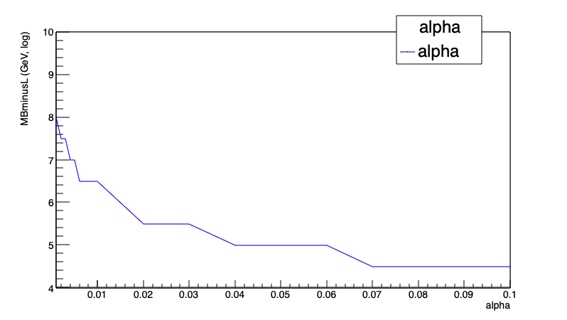
Figure 7: The lowest value of $M_{B-L}$ consistent with both electron EDM and baryon asymmetry experiments plotted as a function of $\alpha$.

It turns out that the lowest allowed value of $M_{B-L}$ is hardly sensitive to the mass parameters and variations in wall thickness and wall velocity. Thus, by scanning the parameter space we can conclude that for consistency with both electron EDM and baryon asymmetry experiments, the scale $M_{B-L}$ of $B-L$-symmetry breaking must be larger than $10^{4.5}\,\mathrm{GeV}$, and over the whole allowed range must be significantly less that $M_{B-L}^{2}/M_{EW}$. These novel bounds provide the most stringent constraints on the parameter space of LRSUSY by far.

More interestingly, our implication that $M_{R}$ must be significantly less than $M_{B-L}^{2}/M_{EW}$ accords with the simplifying proposal of Aulakh et al. Aulakh:1997fq viz. $M_{R}\gtrsim M_{B-L}^{2}/M_{EW}$, as discussed at (14), only at the lowest allowed value of $M_{B-L}$. Aulakh et al.’s proposal arose from gravity mediated TeV scale SUSY breaking where the gravitino is not much heavier than $M_{EW}$. Within the validity of this proposal this analysis makes a specific prediction of the $M_{B-L}$ and hence the $M_{R}$. Since LHC has not discovered any signatures of SUSY, TeV scale SUSY breaking is now a highly unlikely possibility though an exciting one to confirm if true.

On the other hand we can reject the $R$ charge proposed in Aulakh:1997fq , in order to allow the fact that the scale of parity breaking and $(B-L)$-symmetry breaking are not maximally far apart. The parameter $m_{\Omega}$ could then be intrinsic to the superpotential. In this case our results are perfectly consistent with PeV scale supersymmetry Wells also considered in the recent work Dhuria , where the gravitino can be much heavier. This places LRSUSY outside the experimental reach of colliders in the near future. On the other hand, the discovery of a non-zero electron EDM value can be taken to be a hint to a narrow range for the $M_{R}$ scale assuming a world with a renormalisable supersymmetric left-right model. Finally it is interesting that two very different low-energy probes viz. baryon asymmetry and electron EDM provide a strong constraint on the allowed parameter space of LRSUSY.

Appendix A Euler-Lagrange equations for spatially varying Higgs vevs

The Euler-Lagrange equations are written explicitly below, where $\ddot{f}$ represents the double derivative of vev of field $f$ with respect to $x$ and $F_{(\Phi_{i})_{j}}$ denotes the $(j,j)$ matrix element of the vev $\langle F_{\Phi_{i}}\rangle$. The expressions for the vevs of the F-terms and D-terms can be found in Equations 8 and 6 respectively. There are eight bidoublet field vevs $r_{1},i_{1},\ldots,r_{2}^{\prime},i_{2}^{\prime}$ which are the real and imaginary parts of the vev $k_{1},\ldots,k_{2}^{\prime}$ respectively. There are 4 triplet fields vevs viz. $d$, $\bar{d}$, $d_{c}$, $\bar{d}_{c}$. All these vevs vary as a function of distance $x$ from the centre of the wall, but we write field $f$ in the equations below and not $f(x)$ for clarity of notation. The vevs of the fields $\omega(x)$, $\omega_{c}(x)$ below take their values from the ansatz in Equation (23).

$$\begin{array}[]{r c l}\ddot{r}_{1}&=&4\alpha\mathrm{Re}(F_{\Omega}+F_{\Omega_{c}})r_{2}^{\prime}+8\alpha\mathrm{Im}(F_{\Omega})i_{2}^{\prime}+8\mu_{11}\mathrm{Re}(F_{(\Phi_{1})_{2}})+8(\mu_{12}+\alpha(\omega-\omega_{c}))\mathrm{Re}(F_{(\Phi_{2})_{2}})\\ &&{}+8g^{2}r_{1}D_{L,3}-2\mu_{1}^{2}r_{1}-4\mu_{3}^{2}(r_{1}^{\prime}\cos\beta_{3}+i_{1}^{\prime}\sin\beta_{3})-2\mu_{5}^{2}(r_{2}^{\prime}\cos\beta_{5}+i_{2}^{\prime}\sin\beta_{5}),\\ \ddot{i}_{1}&=&-4\alpha\mathrm{Re}(F_{\Omega}+F_{\Omega_{c}})i_{2}^{\prime}+8\alpha\mathrm{Im}(F_{\Omega})r_{2}^{\prime}+8\mu_{11}\mathrm{Im}(F_{(\Phi_{1})_{2}})+8(\mu_{12}+\alpha(\omega-\omega_{c}))\mathrm{Im}(F_{(\Phi_{2})_{2}})\\ &&{}+8g^{2}i_{1}D_{L,3}-2\mu_{1}^{2}i_{1}-4\mu_{3}^{2}(-i_{1}^{\prime}\cos\beta_{3}+r_{1}^{\prime}\sin\beta_{3})-2\mu_{5}^{2}(-i_{2}^{\prime}\cos\beta_{5}+r_{2}^{\prime}\sin\beta_{5}),\\ \ddot{r}_{2}&=&-4\alpha\mathrm{Re}(F_{\Omega}+F_{\Omega_{c}})r_{1}^{\prime}-8\alpha\mathrm{Im}(F_{\Omega})i_{1}^{\prime}+8(\mu_{12}-\alpha(\omega-\omega_{c}))\mathrm{Re}(F_{(\Phi_{1})_{2}})+8\mu_{22}\mathrm{Re}(F_{(\Phi_{2})_{2}})\\ &&{}+8g^{2}r_{2}D_{L,3}-2\mu_{2}^{2}r_{2}-4\mu_{4}^{2}(r_{2}^{\prime}\cos\beta_{4}+i_{2}^{\prime}\sin\beta_{4})-2\mu_{5}^{2}(r_{1}^{\prime}\cos\beta_{5}+i_{1}^{\prime}\sin\beta_{5}),\\ \ddot{i}_{2}&=&4\alpha\mathrm{Re}(F_{\Omega}+F_{\Omega_{c}})i_{1}^{\prime}-8\alpha\mathrm{Im}(F_{\Omega})r_{1}^{\prime}+8(\mu_{12}-\alpha(\omega-\omega_{c}))\mathrm{Im}(F_{(\Phi_{1})_{2}})+8\mu_{22}\mathrm{Im}(F_{(\Phi_{2})_{2}})\\ &&{}+8g^{2}i_{2}D_{L,3}-2\mu_{2}^{2}i_{2}-4\mu_{4}^{2}(-i_{2}^{\prime}\cos\beta_{4}+r_{2}^{\prime}\sin\beta_{4})-2\mu_{5}^{2}(-i_{1}^{\prime}\cos\beta_{5}+r_{1}^{\prime}\sin\beta_{5}),\\ \ddot{r}^{\prime}_{1}&=&-4\alpha\mathrm{Re}(F_{\Omega}+F_{\Omega_{c}})r_{2}-8\alpha\mathrm{Im}(F_{\Omega})i_{2}+8\mu_{11}\mathrm{Re}(F_{(\Phi_{1})_{1}})+8(\mu_{12}-\alpha(\omega-\omega_{c}))\mathrm{Re}(F_{(\Phi_{2})_{1}})\\ &&{}-8g^{2}r_{1}^{\prime}D_{L,3}-2\mu_{1}^{2}r_{1}^{\prime}-4\mu_{3}^{2}(r_{1}\cos\beta_{3}+i_{1}\sin\beta_{3})-2\mu_{5}^{2}(r_{2}\cos\beta_{5}+i_{2}\sin\beta_{5}),\\ \ddot{i}^{\prime}_{1}&=&4\alpha\mathrm{Re}(F_{\Omega}+F_{\Omega_{c}})i_{2}-8\alpha\mathrm{Im}(F_{\Omega})r_{2}+8\mu_{11}\mathrm{Im}(F_{(\Phi_{1})_{1}})+8(\mu_{12}-\alpha(\omega-\omega_{c}))\mathrm{Im}(F_{(\Phi_{2})_{1}})\\ &&{}-8g^{2}i_{1}^{\prime}D_{L,3}-2\mu_{1}^{2}i_{1}^{\prime}-4\mu_{3}^{2}(-i_{1}\cos\beta_{3}+r_{1}\sin\beta_{3})-2\mu_{5}^{2}(-i_{2}\cos\beta_{5}+r_{2}\sin\beta_{5}),\\ \ddot{r}^{\prime}_{2}&=&4\alpha\mathrm{Re}(F_{\Omega}+F_{\Omega_{c}})r_{1}+8\alpha\mathrm{Im}(F_{\Omega})i_{1}+8(\mu_{12}+\alpha(\omega-\omega_{c}))\mathrm{Re}(F_{(\Phi_{1})_{1}})+8\mu_{22}\mathrm{Re}(F_{(\Phi_{2})_{1}})\\ &&{}-8g^{2}r_{2}^{\prime}D_{L,3}-2\mu_{2}^{2}r_{2}^{\prime}-4\mu_{4}^{2}(r_{2}\cos\beta_{4}+i_{2}\sin\beta_{4})-2\mu_{5}^{2}(r_{1}\cos\beta_{5}+i_{1}\sin\beta_{5}),\\ \ddot{i}^{\prime}_{2}&=&-4\alpha\mathrm{Re}(F_{\Omega}+F_{\Omega_{c}})i_{1}+8\alpha\mathrm{Im}(F_{\Omega})r_{1}+8(\mu_{12}+\alpha(\omega-\omega_{c}))\mathrm{Im}(F_{(\Phi_{1})_{1}})+8\mu_{22}\mathrm{Im}(F_{(\Phi_{2})_{1}})\\ &&{}-8g^{2}i_{2}^{\prime}D_{L,3}-2\mu_{2}^{2}i_{2}^{\prime}-4\mu_{4}^{2}(-i_{2}\cos\beta_{4}+r_{2}\sin\beta_{4})-2\mu_{5}^{2}(-i_{1}\cos\beta_{5}+r_{1}\sin\beta_{5}).\end{array}$$ (36)

$$\begin{array}[]{rcl}\ddot{d}&=&2a\mathrm{Re}(F_{\Omega})\bar{d}+2F_{\bar{\Delta}}(m_{\Delta}+a\omega),\\ \ddot{\bar{d}}&=&2a\mathrm{Re}(F_{\Omega})d+2F_{\Delta}(m_{\Delta}+a\omega),\\ \ddot{d}_{c}&=&2a\mathrm{Re}(F_{\Omega_{c}})\bar{d}_{c}+2F_{\bar{\Delta_{c}}}(m_{\Delta}+a\omega_{c}),\\ \ddot{\bar{d}}_{c}&=&2a\mathrm{Re}(F_{\Omega_{c}})d_{c}+2F_{\Delta_{c}}(m_{\Delta}+a\omega_{c}).\end{array}$$ (37)

Appendix B Temperature dependent mass matrix of neutral bidoublet Higgs

Here we display the temperature dependent mass matrix corresponding to Equations 16, 17. This is a symmetric $8\times 8$ matrix in the fields $r_{1}$, $i_{1}$, $r_{2}$, $i_{2}$, $r^{\prime}_{1}$, $i^{\prime}_{1}$, $r^{\prime}_{2}$, $i^{\prime}_{2}$. The mass parameters $\mu$ are assumed to be corrected for the temperature of $T=M_{B-l}$. Following Cline2HDM , we can write the matrix with the zero temperature Debye mass corrections as shown below. In obtaining the domain wall profiles we use $T=0$ and for the electron EDM calculation we use $T=M_{B-L}$.

$$\begin{array}[]{rcl}M_{r_{1},r_{1}}&=&M_{i_{1},i_{1}}=\mu_{11}^{2}+(\mu_{12}-\alpha M_{R})^{2}-\mu_{1}^{2}-\frac{g^{2}T^{2}}{6}\\ M_{r_{2},r_{2}}&=&M_{i_{2},i_{2}}=(\mu_{12}+\alpha M_{R})^{2}+\mu_{22}^{2}-\mu_{2}^{2}-\frac{g^{2}T^{2}}{6}\\ M_{r^{\prime}_{1},r^{\prime}_{1}}&=&M_{i^{\prime}_{1},i^{\prime}_{1}}=\mu_{11}^{2}+(\mu_{12}+\alpha M_{R})^{2}-\mu_{1}^{2}-\frac{g^{2}T^{2}}{6}\\ M_{r^{\prime}_{2},r^{\prime}_{2}}&=&M_{i^{\prime}_{2},i^{\prime}_{2}}=(\mu_{12}-\alpha M_{R})^{2}+\mu_{22}^{2}-\mu_{2}^{2}-\frac{g^{2}T^{2}}{6}\\ &&\\ M_{r_{1},i_{1}}&=&M_{r_{2},i_{2}}=M_{r^{\prime}_{1},i^{\prime}_{1}}=M_{r^{\prime}_{2},i^{\prime}_{2}}=M_{r_{1},i_{2}}=M_{i_{1},r_{2}}=M_{r^{\prime}_{1},i^{\prime}_{2}}=M_{i^{\prime}_{1},r^{\prime}_{2}}=0\\ &&\\ M_{r_{1},r_{2}}&=&\mu_{11}(\mu_{12}+\alpha M_{R})+(\mu_{12}-\alpha M_{R})\mu_{22}\\ M_{i_{1},i_{2}}&=&\mu_{11}(\mu_{12}+\alpha M_{R})+(\mu_{12}-\alpha M_{R})\mu_{22}\\ M_{r^{\prime}_{1},r^{\prime}_{2}}&=&\mu_{11}(\mu_{12}-\alpha M_{R})+(\mu_{12}+\alpha M_{R})\mu_{22}\\ M_{i^{\prime}_{1},i^{\prime}_{2}}&=&\mu_{11}(\mu_{12}-\alpha M_{R})+(\mu_{12}+\alpha M_{R})\mu_{22}\\ &&\\ M_{r_{1},r^{\prime}_{1}}&=&-M_{i_{1},i^{\prime}_{1}}=-2\mu_{3}^{2}\cos\beta_{3}\\ M_{r_{1},i^{\prime}_{1}}&=&-M_{i_{1},r^{\prime}_{1}}=-2\mu_{3}^{2}\sin\beta_{3}\\ &&\\ M_{r_{1},r^{\prime}_{2}}&=&-M_{i_{1},i^{\prime}_{2}}=M_{r_{2},r^{\prime}_{1}}=-M_{i_{2},i^{\prime}_{1}}=-\mu_{5}^{2}\cos\beta_{5}\\ M_{r_{1},i^{\prime}_{2}}&=&M_{i_{1},r^{\prime}_{2}}=M_{r_{2},i^{\prime}_{1}}=M_{i_{2},r^{\prime}_{1}}=-\mu_{5}^{2}\sin\beta_{5}\\ &&\\ M_{r_{2},r^{\prime}_{2}}&=&-M_{i_{2},i^{\prime}_{2}}=-2\mu_{4}^{2}\cos\beta_{4}\\ M_{r_{2},i^{\prime}_{2}}&=&-M_{i_{2},r^{\prime}_{2}}=-2\mu_{4}^{2}\sin\beta_{4}\end{array}$$ (38)

References

• (1) A.Β D. Sakharov, β€œViolation of CP invariance, C asymmetry and baryon asymmetry of the Universe,” Pisma Zh. Eksp. Teor. Fiz., vol.Β 5, pp.Β 32––35, 1967. [JETP Lett. 5 (1967) 24].
• (2) V.Β Kuzmin, V.Β Rubakov, and M.Β Shaposhnikov, β€œOn the anomalous electroweak baryon number nonconservation in the early Universe,” Phys. Lett. B, vol.Β 155, pp.Β 36–42, 1985.
• (3) K.Β Kajantie, M.Β Laine, K.Β Rummukainen, and M.Β Shaposhnikov, β€œIs there a hot electroweak phase transition at $m_{h}\approx m_{w}$?,” Phys. Rev. Lett., vol.Β 77, pp.Β 2887–2890, 1996.
• (4) K.Β Kajantie, M.Β Laine, K.Β Rummukainen, and M.Β Shaposhnikov, β€œA non-perturbative analysis of the finite T phase transition in $\mathrm{SU}(2)\times\mathrm{U}(1)$ electroweak theory,” Nucl. Phys. B, vol.Β 493, pp.Β 413–438, 1997.
• (5) F.Β Csikor, Z.Β Fodor, and J.Β Heitger, β€œEndpoint of the hot electroweak phase transition,” Phys. Rev. Lett., vol.Β 82, no.Β 1, pp.Β 21–24, 1999.
• (6) ATLAS Collaboration, β€œObservation of a new particle in the search for the Standard Model Higgs boson with the ATLAS detector at the LHC,” Phys. Lett. B, vol.Β 716, no.Β 1, pp.Β 1–29, 2012.
• (7) CMS Collaboration, β€œObservation of a new boson at a mass of 125 GeV with the CMS experiment at the LHC,” Phys. Lett. B, vol.Β 716, no.Β 1, pp.Β 30–61, 2012.
• (8) M.Β Gavela, P.Β Hernandez, J.Β Orloff, O.Β Pene, and C.Β Quimbay, β€œStandard model CP-violation and baryon asymmetry (II). Finite temperature,” Nucl. Phys. B, vol.Β 430, no.Β 2, pp.Β 382–426, 1994.
• (9) R.Β Mohapatra and G.Β SenjanoviΔ‡, β€œNeutrino masses and mixings in gauge models with spontaneous parity violation,” Physical Review D, vol.Β 23, no.Β 1, pp.Β 165–180, 1981.
• (10) R.Β Kuchimanchi and R.Β Mohapatra, β€œNo parity violation without r-parity violation,” Physical Review D, vol.Β 48, no.Β 9, pp.Β 4352–4360, 1993.
• (11) C.Β S. Aulakh, K.Β Benakli, and G.Β Senjanovic, β€œReconciling supersymmetry and left-right symmetry,” Phys. Rev. Lett., vol.Β 79, pp.Β 2188–2191, 1997.
• (12) C.Β Aulakh, A.Β Melfo, A.Β RaΕ‘in, and G.Β SenjanoviΔ‡, β€œSupersymmetry and large scale left-right symmetry,” Physical Review D, vol.Β 58, pp.Β 115007:1 – 115007:12, 1998.
• (13) J.Β Cline, U.Β Yajnik, S.Β Nayak, and M.Β Rabikumar, β€œTransient domain walls and lepton asymmetry in the left-right symmetric model,” Phys. Rev. D, vol.Β 66, pp.Β 065001:1–065001:11, 2002.
• (14) A.Β Sarkar, Abhishek, and U.Β Yajnik, β€œPeV scale left–right symmetry and baryon asymmetry of the Universe,” Nucl. Phys. B, vol.Β 800, pp.Β 253–269, 2008.
• (15) L.Β Canetti, M.Β Drewes, and M.Β Shaposhnikov, β€œMatter and antimatter in the universe,” New Journal of Physics, vol.Β 14, pp.Β 095012:1–095012:20, 2012.
• (16) Y.Β Yamaguchi and N.Β Yamanaka, β€œLarge long-distance contributions to the electric dipole moments of charged leptons in the standard model,” Phys. Rev. Lett., vol.Β 125, pp.Β 241802:1–241802:7, 2020. Also available at arXiv:2003.08195. Full version at arXiv:2006.00281.
• (17) ACME Collaboration, β€œImproved limit on the electric dipole moment of the electron,” Nature, vol.Β 562, pp.Β 355–364, 2018.
• (18) J.Β Nieves, D.Β Chang, and P.Β Pal, β€œElectric dipole moment of the electron in left-right-symmetric theories,” Physical Review D, vol.Β 33, pp.Β 3324–3328, 1986.
• (19) F.Β Xu, H.Β An, and X.Β Ji, β€œNeutron electric dipole moment constraint on scale of minimal left-right symmetric model,” Journal of High Energy Physics, pp.Β 88:1–88:21, 2010.
• (20) M.Β Frank, β€œElectric dipole moment of the electron in the left-right supersymmetric model,” Physical Review D, vol.Β 59, pp.Β 055006:1–055006:12, 1999.
• (21) M.Β Frank, β€œThe electric dipole moment of the neutron in the left-right supersymmetric model,” Journal of Physics G: Nuclear and Particle Physics, vol.Β 25, no.Β 9, pp.Β 1813–1828, 1999.
• (22) S.Β Barr and A.Β Zee, β€œElectric dipole moment of the electron and of the neutron,” Phys. Rev. Lett., vol.Β 65, no.Β 1, pp.Β 21–24, 1990.
• (23) N.Β Chen, T.Β Li, Z.Β Teng, and Y.Β Wu, β€œCollapsing domain walls in the two-Higgs-doublet model and deep insights from the EDM,” Journal of High Energy Physics, pp.Β 081:0–081:30, 2020.
• (24) S.Β Mishra and U.Β Yajnik, β€œSpontaneously broken parity and consistent cosmology with transitory domain walls,” Physical Review D, vol.Β 81, pp.Β 045010:1–045010:13, 2010.
• (25) L.Β Dolan and R.Β Jackiw, β€œSymmetry behavior at finite temperature,” Physical Review D, vol.Β 9, pp.Β 3320–3341, 1974.
• (26) J.Β Cline, K.Β Kainulainen, and M.Β Trott, β€œElectroweak baryogenesis in two higgs doublet models and b meson anomalies,” Journal of High Energy Physics, pp.Β 089:0–089:47, 2011.
• (27) G.Β Anderson and L.Β Hall, β€œElectroweak phase transition and baryogenesis,” Phys. Rev. D, vol.Β 45, pp.Β 2685–2698, 1992.
• (28) D.Β Morrissey and M.Β Ramsey-Musolf, β€œElectroweak baryogenesis,” New Journal of Physics, vol.Β 14, pp.Β 125003:1–125003:39, 2012.
• (29) L.Β Fromme, S.Β Huber, and M.Β Seniuch, β€œBaryogenesis in the two-Higgs doublet model,” Journal of High Energy Physics, pp.Β 038:0–038:25, 2006.
• (30) C.Β Wainwright, β€œCosmotransitions: computing cosmological phase transition temperatures and bubble profiles with multiple fields,” Comput. Phys. Comm., vol.Β 183, pp.Β 2006–2013, 2012.
• (31) D.Β Chang, W.-Y. Keung, and T.Β Yuan, β€œTwo-loop bosonic contribution to the electron electric dipole moment,” Phys. Rev. D, vol.Β 43, no.Β 1, pp.Β 43:R14–43:R16, 1991.
• (32) R.Β Mohapatra and X.Β Zhang, β€œElectroweak baryogenesis in left-right-symmetric models,” Physical Review D, vol.Β 46, pp.Β 5331–5336, 1992.
• (33) J.-M. Frβ€˜ere, L.Β Houart, J.Β Moreno, J.Β Orloff, and M.Β Tytgat, β€œGeneration of the baryon asymmetry of the universe within the left-right symmetric model,” Physics Letters B, vol.Β 314, pp.Β 289–297, 1993.
• (34) P.Β Banerjee and U.Β Yajnik, β€œNew ultraviolet operators in supersymmetric so(10) gut and consistent cosmology,” Physical Review D, vol.Β 101, pp.Β 075041:1–075041:12, 2020.
• (35) M.Β Joyce, T.Β Prokopec, and N.Β Turok, β€œNonlocal electroweak baryogenesis. ii. the classical regime,” Physical Review D, vol.Β 53, pp.Β 2958–2980, 1996.
• (36) J.Β Cline, M.Β Joyce, and K.Β Kainulainen, β€œSupersymmetric electroweak baryogenesis,” Journal of High Energy Physics, pp.Β 018:0–018:50, 2000. Also the errata published in the same volume.
• (37) I.Β Esteban, M.Β Gonzalez-Garcia, M.Β Maltoni, T.Β Schwetz, and A.Β Zhou, β€œThe fate of hints: updated global analysis of three-flavor neutrino oscillations.” Available at arXiv::2007.14792, 2020.
• (38) J.Β Wells, β€œPeV-scale supersymmetry,” Physical Review D, vol.Β 71, pp.Β 015013:1–015013:5, 2005.
• (39) M.Β Dhuria and V.Β Rentala, β€œPeV scale supersymmetry breaking and the IceCube neutrino flux,” Journal of High Energy Physics, pp.Β 004:0–004:35, 2018.