The evolution of the low-density H i intergalactic medium from $z$ $=$ 3.6 to 0: Data, transmitted flux and H i column density

Abstract

We present a new, uniform analysis of the H i transmitted flux ($F$) and H i column density ($N_{\mathrm{{\mathrm{H\,\mathsc{i}}}}}$) distribution in the low-density IGM as a function of redshift $z$ for 0 $<$ $z$ $<$ 3.6 using 55 HST/COS FUV ($\Delta z$ $=$ 7.2 at $z$ $<$ 0.5), five HST/STIS+COS NUV ($\Delta z$ $=$ 1.3 at $z$ $\sim$ 1) and 24 VLT/UVES and Keck/HIRES ($\Delta z$ $=$ 11.6 at 1.7 $<$ $z$ $<$ 3.6) AGN spectra. We performed a consistent, uniform Voigt profile analysis to combine spectra taken with different instruments, to reduce systematics and to remove metal-line contamination. We confirm previously known conclusions on firmer quantitative grounds in particular by improving the measurements at $z$ $\sim$ 1. Two flux statistics at 0 $<$ $F$ $<$ 1, the mean H i flux and the flux probability distribution function (PDF), show that considerable evolution occurs from $z$ $=$ 3.6 to $z$ $=$ 1.5, after which it slows down to become effectively stable for $z$ $<$ 0.5. However, there are large sightline variations. For the H i column density distribution function (CDDF, $f$ $\propto$ $N_{{\mathrm{H\,\mathsc{i}}}}^{-\beta}$) at $\log(N_{\mathrm{{\mathrm{H\,\mathsc{i}}}}}/1\,{\mathrm{cm}^{-2}})$ $\in$ [13.5, 16.0], $\beta$ increases as $z$ decreases from $\beta\!=\!1.60$ at $z$ $\sim$ 3.4 to $\beta$ $=$ 1.82 at $z$ $\sim$ 0.1. The CDDF shape at lower redshifts can be reproduced by a small amount of clockwise rotation of a higher-$z$ CDDF with a slightly larger CDDF normalisation. The absorption line number per $z$ ($dn/dz$) shows a similar evolutionary break at $z$ $\sim$ 1.5 as seen in the flux statistics. High-$N_{\mathrm{{\mathrm{H\,\mathsc{i}}}}}$ absorbers evolve more rapidly than low-$N_{\mathrm{{\mathrm{H\,\mathsc{i}}}}}$ absorbers to decrease in number or cross-section with time. The individual $dn/dz$ shows a large scatter at a given $z$. The scatter increases toward lower $z$, possibly caused by a stronger clustering at lower $z$.

1 Introduction

The small amount of neutral hydrogen (H i) in the diffuse, warm ($\sim\!10^{4}$ K), highly ionised intergalactic medium (IGM) produces a rich series of narrow absorption lines blueward of the Ly$\alpha$ emission line in the spectra of AGN, also known as the Ly$\alpha$ forest. Combined with theory and state-of-art cosmological, hydrodynamic simulations, the evolution of the Ly$\alpha$ forest over cosmic time provides some of the most powerful cosmological and astrophysical constraints as 1) hydrogen is the most abundant element and a mostly unbiased basic building block of stars and galaxies, 2) the forest is the largest reservoir of baryons at all epochs, 3) it traces the underlying dark matter in a simple manner, thus outlining the skeleton of the large-scale structure, 4) its thermal state provides clues on the reionisation history, and 5) it contains information on galaxy formation and evolution through the gas infall from the surrounding IGM and galactic feedback (Sargent et al. 1980; Cen et al. 1994; Weymann et al. 1998; Schaye 2001; Lehner et al. 2007; Davé et al. 2010; Shen et al. 2012; Ford et al. 2013; Danforth et al. 2016; Martizzi et al. 2019).

The physics of the Ly$\alpha$ forest is largely determined by a combination of the Hubble expansion, the changes in the ionising UV background radiation field (UVB) and the formation and evolution of the large-scale structure and galaxies. The Hubble expansion cools the gas adiabatically and decreases the gas density and the recombination rate. This process is fairly well-constrained by the cosmological parameters from WMAP and Planck observations (Jarosik et al. 2011; Planck collaboration 2016).

On the other hand, the UVB assumed to originate primarily from AGN and in some degree also from star-forming galaxies photoionises and heats the IGM. If the intensity of the UVB decreases, the H i fraction increases. Unfortunately, the UVB and its evolution are less well constrained both theoretically and observationally. The relative contributions from AGN and galaxies are poorly known as a function of redshift, in part since the escape fraction of H i ionising photons and the amount of dust attenuation of galaxies is uncertain and since the AGN spectral energy distribution including both obscured and unobscured AGN is poorly constrained. The process of the photoionisation and recombination of the integrated UV emission through the clumpy, opaque IGM is also complex (Bolton et al. 2005; Faucher-Giguère et al. 2008b; Haardt & Madau 2012; Kollmeier et al. 2014; Khaire & Srianand 2019; Puchwein et al. 2019; Faucher-Giguère 2020). At the same time, outflows from star formation and AGN activity change the dynamical, chemical and thermal states of galaxy halos and the surrounding IGM, slowing down the gas infall (Davé et al. 2010; Steidel et al. 2010; Suresh et al. 2015). In addition, structure evolution is expected to create collisionally-ionised hot gas known as the Warm-Hot Intergalactic Medium (WHIM) with temperature $\sim\!10^{5-7}$ K through gravitational shock heating. The WHIM becomes a more dominant phase at $z\!<\!1$ and could hide a large fraction of missing baryons (Fukugita et al. 1998; Cen & Ostriker 1999; Savage et al. 2014; Haider et al. 2016).

All of these physical processes leave their footprints on the evolutionary properties of the diffuse IGM in the expanding universe through the shape and number of absorption profiles. The H i column density $N_{\mathrm{{\mathrm{H\,\mathsc{i}}}}}$ is determined by a combination of the neutral fraction of photoionised hydrogen, the gas density and the UVB, while the absorption line width constrains the temperature and non-thermal turbulent motion of the IGM.

At 1.5 $<$ $z$ $<$ 3.6, the evolution of the Ly$\alpha$ forest is well-established observationally from the Voigt profile fitting analysis of high-resolution and high signal-to-noise (S/N) ground-based optical QSO spectra taken with instruments such as the HIRES (HIgh-Resolution Echelle Spectrometer, Vogt (1994, 2002)) on Keck I and the UVES (UV-Visible Echelle Spectrograph, Dekker et al. (2000)) on the VLT (Very Large Telescope), as the H i absorption lines at $N_{\mathrm{{\mathrm{H\,\mathsc{i}}}}}\!\leq\!10^{17}$ cm^-2 are usually fully resolved.

At $z$ $<$ 1.5, the H i Ly$\alpha$ can be observed only in the UV region from space due to the atmospheric cutoff at $\sim$3050 Å. Before the installation of COS (Cosmic Origins Spectrograph) onboard HST in 2009, the low sensitivity of available UV spectrographs such as HST/STIS (Space Telescope Imaging Spectrograph) had seriously limited the sample size and data quality, hindering a consistent analysis of the IGM combined at $z$ $>$ 1.5 from optical data and at $z$ $<$ 1.5 from UV data (Weymann et al. 1998; Janknecht et al. 2006; Lehner et al. 2007). With its factor of $\sim$10 higher throughput than STIS, COS has opened a new era for the low-$z$ IGM study from a unprecedented large number of good-quality AGN spectra (Danforth et al. 2016). Although the COS G130M/G160M grating has a factor of 3 lower resolution ($\sim$ 19  km s^-1) than the UVES/HIRES resolution, most low-$z$ H i lines are resolved at the COS resolution (Fig. 1) and line blending is not as problematic as at $z$ $>$ 1.

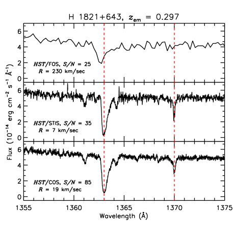
Figure 1: Comparisons of H 1821+643 spectra taken with HST/FOS (upper panel, from the HST archive for high-level products), HST/STIS (middle panel, Wakker & Savage (2009)) and HST/COS (lower panel, taken at Lifetime Position 1). The low-resolution FOS spectrum does not show an asymmetric profile of the H i Ly$\alpha$ at 1363 Å as convincingly as STIS E140M and COS G130M spectra. Two weak absorption lines with $\log N_{\mathrm{{\mathrm{H\,\mathsc{i}}}}}\!\sim\!12.65$ are clearly present at 1366.2 Å and 1368.4 Å in the higher-S/N COS spectrum. Being usually much narrower than H i, most metal lines are not resolved at the COS resolution, as seen in the profiles of Galactic ISM Ni ii $\lambda$1370.13 from STIS and COS.

Here in the first of a series from our ongoing observational study on the redshift evolution of the IGM, we present the properties of the transmitted flux $F$ at 0 $<$ $F$ $<$ 1 and H i column density $N_{\mathrm{{\mathrm{H\,\mathsc{i}}}}}$ at $N_{\mathrm{{\mathrm{H\,\mathsc{i}}}}}$ $\in$ [13.5, 17] of the low-density intergalactic H i from $z$ $=$ 3.6 to $z$ $=$ 0, i.e. since the universe was 1.8 Gyr old. We constructed a high-quality IGM sample from three public archives: 55 HST/COS FUV G130M/G160M AGN spectra covering the Ly$\alpha$ forest at $z$ $<$ 0.47, two QSO spectra from the HST/STIS E230M archive supplemented with our new observations of three QSOs with the HST/COS NUV G225M grating at $z$ $\sim$ 1 and 24 VLT-UVES/Keck I-HIRES QSO spectra at 1.7 $<$ $z$ $<$ 3.6.

We have performed our own consistent, uniform in-depth Voigt profile fitting analysis to the three data sets, instead of compiling fitted line parameters from literature, cf. Tilton et al. (2012). Although time-intensive, this approach is the only viable option to reduce any systematics, to account for the different spectral characteristics of each spectrograph and to remove metal contamination. One of our primary aims is to provide the fundamental measurements of the low-density IGM from the self-consistent analysis for theoreticians to test cosmological simulations and theories on structure/galaxy formation and evolution.

We produced two sets of the fitted parameters: one using only the Ly$\alpha$ (the Ly$\alpha$-only fit) as most simulations use the Ly$\alpha$ forest region and another using all the available Lyman series (the Lyman series fit) to derive reliable line parameters of saturated Ly$\alpha$ lines. Although the redshift coverage is not continuous and the sample size at $z$ $\sim$ 1 is rather small, the analysed redshift range is the best compromise within the capabilities of currently available ground-based and space-based spectrographs.

This paper is organised as follows. Our data sets are presented in Section 2. The Voigt profile fitting technique and its caveats are discussed in Section 3. The H i continuous flux statistics are found in Section 4. The distribution of H i column densities is discussed in Section 5. We summarise our results in Section 6. All the long tables are published electronically on the MNRAS webpage. Throughout this study, the cosmological parameters are assumed to be the matter density $\Omega_{\mathrm{m}}$ $=$ 0.3, the cosmological constant $\Omega_{\mathrm{\Lambda}}$ $=$ 0.7, and the current Hubble constant $\mathrm{H_{0}}$ $=$ 100 $h$  km s^-1Mpc^-1 with $h$ $=$ 0.7. The logarithm $N_{{\mathrm{H\,\mathsc{i}}}}$ is defined as $\log N_{{\mathrm{H\,\mathsc{i}}}}$ $=$ $\log(N_{{\mathrm{H\,\mathsc{i}}}}/1\,{\mathrm{cm}}^{-2})$. All the quoted S/N ratios are per resolution element. The atomic parameters are taken from the atomic parameter file in the Voigt profile fitting package VPFIT (Carswell & Webb 2014), with some unlisted values from the NIST (National Institute of Standards and Technology) Atomic Spectra Database. We also use the terms “absorbers”, “components” and “absorption lines” interchangeably.

2 Data

2.1 General description of the analysed data

The most physically meaningful analysis of absorption spectra is to decompose absorption lines into discrete components to derive column densities and line widths, assuming the profile shape to be the Voigt function. The commonly used curve-of-growth analysis from the equivalent width measurement is straightforward with the mathematically well-characterised associated error (Ebbets 1995). However, its derived column density is degenerate with the absorption line width for a single-line transition, such as typical IGM H i Ly$\alpha$ with $\log N_{{\mathrm{H\,\mathsc{i}}}}$ $\leq$ 13.5 for which Ly$\beta$ cannot be detected in COS spectra with $S/N$ $\leq$ 25. Since about 60% of IGM H i lines with $\log N_{{\mathrm{H\,\mathsc{i}}}}$ $\in$ [13, 15] at $z$ $\sim$ 0.2 have $\log N_{{\mathrm{H\,\mathsc{i}}}}$ $\leq$ 13.5, inability of constraining the line width, thus the column density in some degree, is a serious drawback of the curve-of-growth analysis. Moreover, deblending of absorption complexes is not straightforward in the curve-of-growth analysis. High-$z$ IGM spectra suffer from severe blending and measuring the equivalent width in high-resolution UVES/HIRES spectra is almost impossible and meaningless.

The Voigt profile fitting analysis requires high-quality spectra in which absorption lines are resolved and deblending is possible. In order to achieve a data quality adequate enough for the profile fitting analysis, we have built the three IGM data sets by selecting good-quality AGN spectra publicly available as of the end of 2017 from HST, FUSE, VLT and Keck archives. Due to the rapid increase of the number of absorption lines with $z$, it is essential to have high-resolution, high-S/N spectra that allow for deblending at $z$ $>$ 1.5. At lower redshifts, high resolution is not as crucial due to much less blending, but a high S/N is still required to place a reliable continuum and to obtain robust fitted line parameters. Our main AGN selection criteria are:

1. Sightlines without damped Ly$\alpha$ systems (DLA, $\log N_{\mathrm{{\mathrm{H\,\mathsc{i}}}}}$ $\geq$ 20.3) in the Ly$\alpha$ forest region and only a few Lyman limit systems ($\log N_{\mathrm{{\mathrm{H\,\mathsc{i}}}}}$ $\geq$ 17.2) in the entire spectrum in order to maximise useful wavelength regions.

2. Spectra covering higher-order H i Lyman lines, at least Ly$\beta$, to obtain a reliable line parameter for saturated Ly$\alpha$ lines. Available FUSE spectra were included to cover the corresponding Lyman series of COS Ly$\alpha$.

3. For COS FUV, STIS and UVES/HIRES spectra, the S/N cut is set to be $\geq$ 18, $\geq$ 18 and $\geq$40 per resolution element in a large fraction of forest regions. This rather arbitrary S/N cut is a compromise between having well measurable lines and as large a sample as possible.

4. To increase the sample size at $z$ $\sim$ 1, we relax the S/N cut and include our three new COS NUV QSO spectra obtained through HST GO program 14265. Two have $S/N$ $\sim$ 15–18, while one has $S/N$ $\sim$ 10–15. Since high-order Lyman regions of the three sightlines are only partly observed, we use these spectra only for the Ly$\alpha$-only analysis. The lower-S/N increases the lowest reliable value for $N_{{\mathrm{H\,\mathsc{i}}}}$ and leads to a unreliable measurement of the transmitted flux (see Section 4.2). However, including the three COS NUV spectra does not change our conclusions.

5. For COS FUV/NUV spectra, a region with S/N lower than each S/N cut is discarded if it is longer than $\sim$5 Å, so as not to compromise the reliable Voigt profile fitting and flux statistics.

6. The forest region with $S/N$ $>$ 18 of the COS FUV spectra is required to be $\geq$ 100 Å wide. This limits the emission redshift to be $z_{\mathrm{em}}$ $>$ 0.1, for which the possible forest coverage is $\geq$ 120 Å. Considering that the forest is $\sim$550 Å long at $z$ $\sim$ 2.5, such a small wavelength coverage makes cosmic variance a major issue. To avoid confusion with high-order Lyman lines in the FUV spectra, the maximum forest $z$ is set to be 0.47.

7. No broad absorption line (BAL) AGN. Mini-BALs are included with the affected wavelength region excluded.

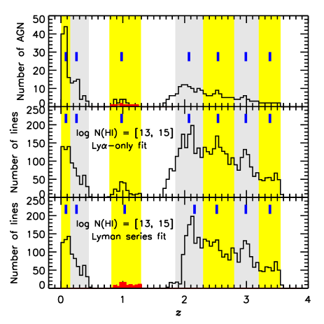
Figure 2: Upper panel: Number of AGN covering the Ly$\alpha$ forest using a $\Delta z$ $=$ 0.05 bin. Any excluded regions due to a low S/N, Milky Way ISM contamination or detector gap are not counted in the number of AGN and IGM H i lines. The red histogram is from the two STIS E230M spectra used for both Ly$\alpha$-only and Lyman series fits. The thick vertical blue lines mark the median $z$ of each redshift bin used for the Ly$\alpha$-only fit. Each redshift bin is shaded as gray and yellow alternatively to clearly distinguish from each other. These bins are chosen to exclude the $z$ range at which the Lyman series fit does not contain enough lines. Middle and lower panels: Number of H i lines from the Ly$\alpha$-only and Lyman series fits, respectively.

The COS FUV (1100–1800 Å), COS NUV (2225–2525 Å), and STIS NUV E230M (1850–3050 Å) spectra contain many Galactic ISM lines, such as Si ii $\lambda\lambda$  1260.42, 1304.37, 1526.70, C ii $\lambda$ 1334.53, Mg ii $\lambda\lambda$, 2796.35, 2803.53, and Fe ii $\lambda\lambda$ 1608.45, 2382.76, 2600.17. The profile fit can easily reveal typical IGM lines blended with ISM lines, if multiple transitions of the same ISM ion are available and if some of the clean transitions are not saturated. However, broad and/or weak blended IGM lines can not be always validated when the spectrum has a low resolution, low S/N or fixed pattern noise. The most noticeable ISM line in the NUV region of our interest is multiple Fe ii including non-saturated transitions so that blended IGM lines above the detection limit are easily detected. However, the COS FUV region contain many single/multiple ISM lines as well as geocoronal emission lines. Therefore, regions contaminated with strong and medium-strength ISM lines are excluded in our IGM study, regardless of available multiple transitions of the same ion.

Our final sample consists of 24 UVES/HIRES QSOs covering the forest at 1.67 $<$ $z$ $<$ 3.56 with the total analyzed $z$ range $\Delta z$ $=$ 11.6, five STIS E230M and COS NUV QSOs at 0.76 $<$ $z$ $<$ 1.30 with $\Delta z$ $=$ 1.3 and 55 COS FUV AGN at 0.00 $<$ $z$ $<$ 0.47 with $\Delta z$ $=$ 7.2. The upper panel of Fig. 2 shows the number of AGN per unit $z$. The thick vertical line notes the median redshift of the seven redshift bins used in this study from the Ly$\alpha$-only fit: $z$ $\in$ [0.00, 0.15] ($\tilde{z}$ $=$ 0.08), [0.15, 0.45] ($\tilde{z}$ $=$ 0.25), [0.78, 1.29] ($\tilde{z}$ $=$ 0.98), [1.85, 2.30] ($\tilde{z}$ $=$ 2.07), [2.30, 2.80] ($\tilde{z}$ $=$ 2.54), [2.80, 3.20] ($\tilde{z}$ $=$ 2.99) and [3.20, 3.55] ($\tilde{z}$ $=$ 3.38), respectively. Median redshift of the seven redshift bins from the Lyman series fit is slightly different as this requires a coverage of the higher-order Lyman lines: $z$ $\in$ [0.00, 0.15] ($\tilde{z}$ $=$ 0.08), [0.15, 0.45] ($\tilde{z}$ $=$ 0.25), [0.82, 1.29] ($\tilde{z}$ $=$ 1.03), [1.85, 2.30] ($\tilde{z}$ $=$ 2.12), [2.30, 2.80] ($\tilde{z}$ $=$ 2.52), [2.80, 3.20] ($\tilde{z}$ $=$ 2.99) and [3.20, 3.55] ($\tilde{z}$ $=$ 3.38), respectively. At $z$ $>$ 1.5, a sightline with less than $\sim$100 Å-long in a redshift bin is excluded to reduce a sightline variation, since each $z$ bin samples a wavelength range with $\geq$400 Å. The middle and lower panels show the number of H i lines at $\log N_{\mathrm{{\mathrm{H\,\mathsc{i}}}}}\!\in\![13,15]$ from the Ly$\alpha$-only fit and Lyman series fits, respectively. The steep decrease of the number of H i lines from the Lyman series fit at $z$ $\sim$ 1.95 is caused by the atmospheric cutoff at 3050 Å in the optical spectra without a corresponding UV spectrum.

Table 1: Analysed UVES/HIRES QSOs

QSOs	$z_{\mathrm{em}}^{a}$	$z_{\mathrm{Ly\alpha}}$	$\lambda\lambda_{\mathrm{Ly\alpha}}$	$\lambda\lambda_{\mathrm{Ly\alpha\beta}}^{\mathrm{b}}$	S/Nc	$\Delta X_{\mathrm{Ly\alpha}}$	$\Delta X_{\mathrm{Ly\alpha\beta}}^{\mathrm{d}}$	Instrument
			(Å)	(Å)	p.r.
HE 1341–1020e	2.1356f	1.667–2.083	3242.0–3748.0	3609.0–3748.0	55–90	1.2289	0.3487	UVES
Q 1101–264g	2.1413	1.659–1.795	3233.0–3398.0	no coverage	45–90	0.3875	no value	UVES
		1.882–2.090	3503.0–3756.0	3607.0–3756.0	65–135	0.6294	0.3740
Q 0122–380	2.1895h	1.700–2.134	3282.0–3810.0	3619.0–3810.0	40–120	1.2941	0.4821	UVES
PKS 1448–232	2.2197	1.716–2.164	3302.0–3846.0	3615.0–3846.0	45–90	1.3399	0.5845	UVES
PKS 0237–23i	2.2219f	1.735–2.169	3325.0–3853.0	3615.0–3853.0	77–137	1.3039	0.6026	UVES
J 2233–6033e	2.2505	1.741–2.197	3332.0–3886.0	3332.0–3886.0j	35–56	1.3729		UVES, STISj
HE 0001–2340k	2.2641	1.752–2.143	3346.0–3821.0	3622.0–3821.0	55–130	1.1720	0.5028	UVES
Q 0109–3518	2.4047	1.873–2.348	3492.6–4070.0	3615.0–4070.0	82–110	1.4725	1.1720	UVES
HE 1122–1648	2.4050	1.891–2.348	3514.0–4070.0	3615.0–4070.0	80–205	1.4205	1.1720	UVES
HE 2217–2818	2.4134	1.886–2.355	3509.0–4078.2	3613.0–4078.2	85–140	1.4545	1.1988	UVES
Q 0329–385	2.4350	1.896–2.378	3521.0–4106.0	3617.0–4106.0	50–80	1.4996	1.2632	UVES
HE 1158–1843e	2.4478	1.940–2.391	3574.5–4122.0	3621.0–4122.0		1.4113	1.2962	UVES
HE 1347–2457	2.6261l	2.058–2.564	3717.5–4333.0		71–116	1.6297		UVES
Q 0453–423e,m	2.6569	2.086–2.260	3752.0–3962.5		70–137	0.5436		UVES
		2.347–2.593	4069.0–4368.4		85–151	0.8151
PKS 0329–255	2.7041n	2.134–2.642	3809.4–4427.0		40–80	1.6574		UVES
Q 0002–422	2.7676	2.183–2.705	3870.0–4504.0		66-145	1.7179		UVES
HE 0151–4326e	2.7810	2.206–2.631	3897.0–4414.0		95–170	1.3949		UVES
HE 2347–4342e	2.8740f	2.333–2.812	4052.4–4634.0		188-278	1.6098		UVES
HE 0940–1050	3.0836	2.452–3.014	4197.0–4880.0		103–145	1.9382		UVES
Q 0420–388o	3.1152p	2.480–3.044	4231.0–4916.0	4455.0–4916.0	103–210	1.9523	1.3321	UVES
Q 0636+6801	3.1752	2.525–3.097	4285.0–4981.0	4532.0–4981.0	65–105	1.9981	1.3084	HIRES
PKS 2126–158	3.2796	2.684–3.208	4479.0–5115.0		100–250	1.8618		UVES
Q 1422+2309	3.6288	2.919–3.552	4764.0–5533.3		122–165	2.3412		HIRES
Q 0055–269	3.6563	2.936–3.562	4785.0–5546.0		80–140	2.3201		UVES

Notes – a: The redshift is measured from the observed Ly$\alpha$ emission line of the QSO. b: The Ly$\alpha$ forest region having a corresponding Ly$\beta$. When left blank, it is the same as $\lambda\lambda_{\mathrm{Ly\alpha}}$. c: S/N per resolution element. d: The absorption line path length corresponding the Ly$\alpha\beta$ forest region. When left blank, it is the same as $\Delta X_{\mathrm{Ly\alpha}}$. e: Mini-BAL (broad absorption line) QSO. f: Due to the intrinsic absorbers around the Ly$\alpha$ emission line of the QSO, the redshift is less accurate. g: A sub-DLA at $z\!=\!1.839$ in the Ly$\alpha$ region. h: The emission feature is rather flat, in addition to several intrinsic absorption lines. The redshift is set to be the position of the highest flux. i: A sub-DLA at $z\!=\!1.673$ in the Ly$\beta$ region. j: The publicly available, science-ready STIS E230M spectrum (Savaglio et al. 1999) covers a high-order Lyman region at 2550–3057 Å. k: A sub-DLA at $z\!=\!2.187$ in the Ly$\alpha$ region. l: The Ly$\alpha$ emission is slightly double-peaked. The redshift is set to the wavelength of the highest flux. m: A sub-DLA at $z\!=\!2.305$ in the Ly$\alpha$ region. n: The emission feature is very flat with several intrinsic absorption lines. The redshift is set to be the center of the flat emission feature. o: A sub-DLA at $z\!=\!3.087$ in the Ly$\alpha$ region causes the flux to be zero at $\leq$3754 Å. p: As the right wing of the sub-DLA at $z\!=\!3.087$ covers the Ly$\alpha$ emission feature in addition to several intrinsic absorbers, the redshift is not accurate.

All the analysed spectra are in the heliocentric velocity frame. In order to avoid the proximity effect, the region of 5,000  km s^-1 blueward of the Ly$\alpha$ emission was excluded. When a sub-DLA with $\log N_{\mathrm{{\mathrm{H\,\mathsc{i}}}}}$ $\in$ [19.0, 20.3] is present in the Ly$\alpha$ forest region, a region of $\pm$50 Å centred at the sub-DLA was discarded, as the low-density H i around sub-DLAs is not likely to represent the typical IGM due to a strong influence by the galaxy producing the sub-DLA.

2.2 UVES and HIRES data

Table 1 lists the 24 QSOs observed with the UVES at the VLT or with the HIRES at Keck I, along with their emission redshift, analysed absorption redshift ranges and S/N per resolution element in the Ly$\alpha$ forest region. The UVES spectra are the same ones analysed by Kim et al. (2007, 2013, 2016), while the HIRES spectra are the same ones described by Boksenberg & Sargent (2015). The UVES and HIRES spectra were sampled at 0.05 Å and 0.04 Å, respectively. Their resolution is about 6.7  km s^-1. Although the S/N differs from QSO to QSO and even varies along the same QSO, the practical $N_{\mathrm{{\mathrm{H\,\mathsc{i}}}}}$ detection limit is $\log N_{\mathrm{{\mathrm{H\,\mathsc{i}}}}}\!\sim$ 12.5.

Table 1 also lists the absorption distance path length, $\Delta X$, which accounts for comoving coordinates at a given $z$ for the adopted cosmology:

$$\Delta X=\int dX=\int\frac{H_{0}}{H(z)}(1+z)^{2}dz,$$ (1)

where $H(z)=100\,h\,[\Omega_{\mathrm{m}}(1+z)^{3}+(1-\Omega_{\mathrm{m}}-\Omega_{\mathrm{\Lambda}})(1+z)^{2}+\Omega_{\mathrm{\Lambda}}]^{\frac{1}{2}}$ (Bahcall & Peebles 1969).

2.3 HST/STIS data

Table 2: Analysed STIS/COS NUV QSOs

QSOs	$z_{\mathrm{em}}^{\mathrm{a}}$	$z_{\mathrm{Ly\alpha}}^{\mathrm{b}}$	$\lambda\lambda_{\mathrm{Ly\alpha}}^{\mathrm{b}}$	$\lambda\lambda_{\mathrm{Ly\alpha\beta}}^{\mathrm{c}}$	Resolving	S/N	$\Delta X_{\mathrm{Ly\alpha}}^{\mathrm{d}}$	Inst	Program ID
			(Å)	(Å)	power	p.r.
PG 1718+481	1.0832	0.783–1.047	2167.0–2489.0	2207.0–2489.0	30,000	18–26	0.5793 (0.5113)	STIS	7292
HE 1211$-$1322	1.121	0.835–1.076	2231.0–2524.0	no coverage	24,000	10-15	0.5113	COS	14265
HE 0331$-$4112	1.124	0.832–1.076	2226.5–2524.0	no coverage	24,000	13–18	0.4935	COS	14265
HS 2154+2228	1.298	0.831–1.076	2225.5–2524.0	no coverage	24,000	$\sim$18	0.5172	COS	14265
PG 1634+706	1.3340	0.981–1.295	2402.5–2789.0	2402.5–2789.0	30,000	34–46	0.7612 (0.7612)	STIS	7292/8312

Notes – a: The redshift with a four decimal place is measured from the Ly$\alpha$ emission line of the QSO, while the one with a three decimal place is from Simbad. b: The Ly$\alpha$ forest region. c: The Ly$\alpha$ forest region covering the corresponding Ly$\beta$. The COS NUV spectra are used only for the Ly$\alpha$-only fit. d: The number in parentheses is $\Delta X$ for the Ly$\alpha\beta$ region. The excluded region due to a very-low S/N of the COS NUV spectra are taken into account.

Due to the low efficiency of STIS E230M, the HST archive offers only one good-quality AGN spectrum covering the forest at $z$ $\sim$ 1, QSO PG 1634+706. The spectrum has $S/N$ $\sim$ 40, comparable to UVES/HIRES data. In order to increase our sample at $z$ $\sim$ 1, PG 1718+481 with the second highest S/N ($\sim$20) is also included (Table 2). These spectra are same as those analysed by Wakker & Savage (2009). The resolution is $\sim$ 10  km s^-1, if the slightly non-Gaussian line spread function (LSF) is approximated as a Gaussian (see more details in Section 3.2). The typical detection limit is $\log N_{\mathrm{{\mathrm{H\,\mathsc{i}}}}}$ $\sim$ 13.0. The pixel size of the final combined STIS spectra continuously increases toward longer wavelengths, $\sim$0.034 Å per pixel at $\sim$2100 Å and $\sim$0.039 Å per pixel at $\sim$2400 Å.

2.4 HST/COS NUV data

The three selected QSOs observed with the COS NUV G225M grating are part of our observing program (HST GO 14265) to study the IGM at $z$ $\sim$ 1 (Table 2). The observations were obtained in TIME-TAG mode in 2015–2016. The central wavelength setting was setup to produce a continuous wavelength coverage at $\sim$2226–2524 Å. To increase the S/N of individual extractions, we ran the COS data reduction pipeline CalCOS version 3.3.4 with a 12-pixel-wide extraction box instead of the CalCOS default 57-pixel extraction box.

Coadding mis-aligned absorption lines due to wavelength calibration errors produces absorption lines artificially broader and smoother. While UVES, HIRES and STIS have a wavelength uncertainty less than 1  km s^-1, the CalCOS wavelength calibration uncertainty is quoted as $\sim$15  km s^-1 (Dashtamirova et al. 2019). In general, the Cal-COS wavelength uncertainty tends to vary with wavelength and becomes larger at the edges of detector segments. A custom-built semi-automatic IDL program was developed to improve the CalCOS wavelength calibration and to coadd the individual CalCOS extractions (Wakker et al. 2015, see their Appendix for details on the COS wavelength re-calibration procedure). We first recalibrate the CalCOS wavelength on a relative scale better than $\sim$5  km s^-1 between the same absorption features by cross-correlating the strong, clean Galactic ISM or IGM lines in all the available, individual extractions of the same QSO in the HST COS/STIS and FUSE archives. The absolute wavelength calibration was further performed using Galactic 21 cm emission toward the QSO by aligning this with the interstellar lines (Wakker et al. 2015). Since the majority of individual extractions have low S/N, it is not always straightforward to align weak/moderate-strength lines in the presence of fixed pattern noise, with the wavelength calibration uncertainty at 5–10  km s^-1. For strong lines, our wavelength recalibration has uncertainty better than 5  km s^-1 in general. However, when absorption lines fall on the edge of the COS detector, their wavelength uncertainty can be at 10–15  km s^-1 occasionally.

The final coadded spectrum is sampled at $\sim$0.034 Å per pixel, slightly smaller at longer wavelengths. The resolution is $\sim$12  km s^-1 with a time-independent non-Gaussian LSF. While the non-Gaussian LSF has an extended wing, the FWHM ($\sim$10.5  km s^-1) at the core is comparable to the one of STIS spectra. Unfortunately, the two QSOs, HE 1211$-$1322 and HE 0331$-$4112, had become fainter at the time of observations compared to earlier low-resolution spectra, causing a lower S/N than the expected $S/N\!\sim\,18$. The region having a much lower S/N than quoted in Table 2 is discarded to keep the spectral quality as high as the data allow. The typical COS NUV $N_{\mathrm{{\mathrm{H\,\mathsc{i}}}}}$ limit is $\log N_{\mathrm{{\mathrm{H\,\mathsc{i}}}}}\!\sim\!13.0$.

The Ly$\beta$ region and the higher-order Lyman regions are not observed or are only observed in part by other UV spectrographs. Since one of the selection criteria is the coverage of the Ly$\beta$ forest, the three NUV G225M spectra are only used for the Ly$\alpha$-only analysis.

Table 3: Analysed COS FUV AGN

AGN	$z_{\mathrm{em}}^{\mathrm{a}}$	$z_{\mathrm{Ly\alpha}},^{\mathrm{b}}$	$\lambda\lambda_{\mathrm{Ly\alpha}}(\lambda\lambda_{\mathrm{Ly\alpha\beta}})^{\mathrm{b}}$	Othersc	Excludedd	S/Ne	$\Delta X_{\mathrm{Ly\alpha}}^{\mathrm{f}}$	LPg	Prog.
		$z_{\mathrm{Ly\alpha\beta}}$	(Å)		region (Å)	p.r.	$\Delta X_{\mathrm{Ly\alpha\beta}}$		ID
PKS 2005–489	0.0711	0.003–0.053	1219.0–1280.5	F(17), D16		26–31	0.0505	LP1	11520
PG 0804+761	0.1002	0.002–0.082	1218.0–1315.0	F(28), D16		45–60	0.0804	LP1	11686
RBS 1897	0.1019	0.003–0.083	1219.0–1317.0	F(11)		31–53	0.0812	LP1	11686
1H 0419–577	0.1045	0.003–0.086	1219.0–1320.0	F(9), D16		33–86	0.0822	LP1	11686, 11692
PKS 2155–304h	$\sim$0.1103i	0.003–0.092	1219.0–1327.0	F(38), D16		30–42	0.0909	LP2	12038
Ton S210	0.1154	0.002–0.096	1218.0–1332.5	F(27), D16		35–50	0.0943	LP1	12204
HE 1228+0131	0.1168j	0.002–0.097	1218.0–1333.5	F(7), D16		40–72	0.0979	LP1	11686
Mrk 106	0.1233	0.003–0.105	1219.0–1343.0	F(10), D16		22–33	0.1006	LP1	12029
IRAS Z06229–6434	0.1290	0.003–0.110	1219.0–1349.5	F(7), D16	1272.3–1292.0	30–37	0.0866	LP1	11692
Mrk 876	0.1291	0.002–0.110	1218.0–1350.0	F(35), D16		58–62	0.1093	LP1	11686, 11524
PG 0838+770	0.1312	0.003–0.112	1219.5–1352.0	F(10), D16		21–40	0.1094	LP1	11520
PG 1626+554	0.1316	0.002–0.113	1218.0–1353.0	F(15), D16		20–35	0.1109	LP1	12029
RX J0048.3+3941	0.1344	0.003–0.115	1219.0–1356.0	F(20), D16		20–36	0.1136	LP1	11686
PKS 0558–504	0.1374	0.002–0.118	1219.0–1359.0	F(25)	1273.4–1300.4	18–23	0.0926	LP1	11692
PG 0026+129h	0.1452	0.003–0.126	1219.0–1369.0	F(7), D16	1270.6–1300.5	18–23	0.0980	LP1	12569
PG 1352+183	0.1508	0.002–0.131	1218.0–1375.5	F(4)	1273.1–1291.0	20–37	0.1191	LP2	13448
PG 1115+407	0.1542j	0.002–0.135	1218.0–1380.0	F(3), D16		20–34	0.1371	LP1	11519
PG 0052+251	0.1544	0.003–0.134	1219.0–1379.0	F(3)		19–33	0.1371	LP3	14268
PG 1307+085h	0.1544	0.003–0.135	1219.0–1380.0	F(6), D16	1295.3–1325.4	20–26	0.1143	LP1	12569
3C 273h	0.1565	0.002–0.135	1218.0–1382.0	F(38), D16		48–82	0.1429	LP1	12038
IRAS F09539–0439h	0.1568	0.003–0.138	1219.0–1383.0	D16	1273.4–1288.1	18–27	0.1265	LP1	12275
		(0.065–0.138)	(1295.0–1383.0)				(0.0763)
Mrk 1014h	0.1631	0.003–0.143	1219.0–1390.0	D16	1300.9–1325.1	18–22	0.1298	LP1	12569
HE 0056–3622	0.1631j	0.002–0.143	1218.0–1390.0	D16	1274.0–1294.0	24–37	0.1306	LP1	12604
		(0.045–0.143)	(1270.0–1390.0)				(0.0882)
IRAS F00040+4325	0.1636	0.003–0.144	1219.0–1391.0	F(5)		18–34	0.1481	LP3	14268
PG 1048+342	0.1667	0.002–0.148	1218.0–1395.0	F(4), D16		18–33	0.1537	LP1	12024
PG 2349–014h	0.1740	0.003–0.154	1219.0–1403.4	F(6), D16	1295.2–1325.5	18–24	0.1378	LP1	12569
PG 1116+215	0.1749	0..002–0.156	1218.0–1405.0	F(25), D16	1301.0–1307.5	33–50	0.1620	LP1	12038
RBS 1768	0.1831	0.003–0.164	1219.0–1415.0		1294.5–1311.0	23–31	0.1623	LP2	12936
PHL 1811	0.1914k	0.006–0.171	1223.0–1424.0	F(24), D16		33–56	0.1786	LP1	12038
PHL 2525	0.2004	0.014–0.180	1233.0–1435.0	F(7), D16	1270.6–1292.0	18–25	0.1634	LP2	12604
RBS 1892	0.2005	0.013–0.180	1231.0–1435.0	D16	1276.0–1306.9	20–28	0.1612	LP2	12604
		(0.084–0.180)	(1318.0–1435.0)				(0.1133)
PG 1121+423	0.2240	0.032–0.203	1255.0–1463.0	D16		18–27	0.1699	LP1	12024
1H 0717+714	$\sim$0.2314i	0.039–0.211	1263.5–1472.0	F(18), D16		28–52	0.1960	LP1	12025
PG 0953+415	0.2331j	0.042–0.221	1267.0–1484.0	F(25), D16		32–52	0.1954	LP1	12038
RBS 567	0.2412	0.078–0.221	1310.5–1484.0	D16		18–25	0.1727	LP1	11520
3C 323.1	0.2649	0.073–0.244	1304.8–1512.0			18–37	0.2091	LP1	12025
PG 1302–102	0.2775	0.078–0.255	1310.0–1526.0	F(20), D16		25–34	0.2203	LP1	12038
4C 25.01	0.2828j	0.084–0.261	1318.0–1533.5		1387.0–1435.5	18–24	0.1691	LP3	14268
Ton 580	0.2901	0.090–0.268	1325.5–1542.0	D16		20–27	0.2232	LP1	11519
H 1821+643	0.2967j	0.099–0.201l	1336.0–1460.0l	F(25), D16		35–80	0.1254	LP1	12038
PG 1001+291	0.3283	0.121–0.298	1363.0–1578.0	F(5), D16		20–27	0.2315	LP1	12038
PG 1216+069	0.3322	0.124–0.310	1366.5–1592.0	F(4), D16		20–33	0.2450	LP1	12025
3C 66A	$\sim$0.3347i	0.128–0.281	1371.5–1557.0	F(2), D16		20–27	0.1983	LP2	12863, 12612
RBS 877	$\sim$0.3373i	0.129–0.267	1373.0–1540.0			18–23	0.1769	LP1	12025
RBS 1795	0.3427	0.133–0.320	1377.5–1605.0	F(4), D16		18–33	0.2499	LP1	11541
MS 0117.2–2837	0.3487j	0.139–0.326	1385.0–1612.0	D16		18–37	0.2502	LP1	12204
PG 1553+113	$\sim$0.4131i	0.193–0.389	1450.0–1689.0	F(15), D16		22–40	0.2776	LP1	11520, 12025
CTS 487	0.4159	0.194–0.300	1452.0–1580.0			18–20	0.1422	LP2	13448
PG 1222+216	0.4333	0.210–0.409	1471.0–1713.0	D16		21–40	0.2877	LP2	12025
HE 0153–4520	0.4496	0.223–0.426	1487.0–1733.0	F(5), D16	1580.0–1614.0	18–36	0.2542	LP1	11541
PG 0003+158	0.4504	0.224–0.426	1488.0–1734.0	D16	1593.0–1617.0	20–27	0.2670	LP1	12038
PG 1259+593	0.4762	0.245–0.452	1514.0–1765.0	F(25), D16		22–36	0.3078	LP1	11541
HE 0226–4110	0.4934	0.261–0.456	1533.0–1770.0	F(28), D16		23–31	0.2973	LP1	11541
PKS 0405–123	0.5726	0.327–0.466	1613.0–1782.5	F(23), D16		27–45	0.2193	LP1	11541, 11508
PG 1424+240	$\sim$0.6035i,m	0.354–0.439	1645.5–1749.0			25–30	0.1330	LP1	12612

Notes – a: The redshift is measured from the observed Ly$\alpha$ emission line of the QSO in the COS FUV spectra. Otherwise, the redshift is taken from NED or Simbad. b: If the $z$/wavelength range of the Ly$\alpha\beta$ region in COS and/or FUSE spectra is different from the Ly$\alpha$ region, it is listed in parenthesis in the next row. c: F–An available FUSE spectrum is used to cover the high-order Lyman lines. The number in parenthesis is a S/N per resolution element at $\sim$1050 Å. D16–The AGN is also included in the low-$z$ COS IGM study in D16, although our adopted AGN naming is often different. d: The wavelength regions with $S/N\!<\!18$ and/or the unobserved regions due to a detector gap. Excluded regions due to the Galactic ISM contamination are not listed. These are Si ii $\lambda$ 1260.42, 1304.37, 1526.70, O i $\lambda$ 1302.16, C ii $\lambda$ 1334.53, Fe ii $\lambda$ 1608.45 and Al ii $\lambda$ 1670.78. When Fe ii $\lambda$ 1608.45 is not saturated and Fe ii $\lambda\lambda$ 1144.93, 1143.22, 1142.36 are covered in G130M, the region at $\sim$1608 Å is included. e: S/N per resolution element. f: The number in parentheses in the next row is $\Delta X$ of the Ly$\alpha\beta$ region. g: The COS FUV Lifetime Position: LP1 – before July 22, 2012, LP2 – from July 23, 2012 to February 8, 2015, LP3 – from February 9, 2015 to October 1, 2017, LP4 – since October 2, 2017. h: Only the G130M spectrum was obtained. i: The AGN is a BL Lac type, showing no conspicuous emission peak. The emission redshift is set to be that of the Ly$\alpha$ absorption at the highest redshift. j: Due to strong intrinsic absorbers on top of the emission peak, the redshift is slightly uncertain. k: The emission peak is relatively flat. The redshift is set to be at the highest flux around the peak. l: The S/N ratio changes abruptly in the forest region: $S/N$ $\geq$ 35 at $\leq$ 1460 Å and $\sim$14–17 at $\geq$ 1460 Å. To satisfy our S/N selection criteria, only the forest region at $\leq$ 1460 Å is included. m: Both NED and Simbad list its redshift as 0.16. However, the STIS E230M spectrum shows that it is a BL Lac type and the redshift is higher than 0.604 from the Ly$\alpha$ absorption features.

2.5 HST/COS FUV data

We select 55 COS G130M/G160M (1100–1800 Å) AGN spectra (Table 3). We note that 44 out of our 55 COS AGN are also included in the COS IGM sample of Danforth et al. (2016, D16 hereafter). However, our analysis methods are different and there is a difference in line identifications and fitted line parameters for $\sim$30% of the lines (see more details in Section 3.4).

All the raw, individual COS exposures were reduced with CalCOS versions 3.0 or 3.1 with the flat-field correction on. Similar to the treatment of COS NUV data as outlined in Section 2.4, we re-calibrated the CalCOS wavelength to an uncertainty better than $\sim$5–10  km s^-1 (Wakker et al. 2015, see their Appendix for details) and coadded the individual extractions sampled at 0.00997 Å (0.01223 Å) per pixel for the G130M (G160M) grating. Since COS spectra are highly oversampled, we binned the final coadded spectrum by 3 pixels, sampled at 0.02991 Å (0.03669 Å) per pixel for the G130M (G160M) grating. The resolving power of each individual extraction is quoted as $R$ $\sim$ 18,000 to 20,000, which corresponds to 15 to 17  km s^-1 for a Gaussian LSF. However, the COS FUV LSF shows the time-dependent non-Gaussianity and the resolving power degraded with time. The spectral resolution can be approximated to $\sim$19  km s^-1 for the COS non-Gaussian LSF at Lifetime Position 1 (see more details in Section 3.2). The wavelength regions contaminated by strong Galactic ISM lines are discarded. The typical COS FUV $N_{\mathrm{{\mathrm{H\,\mathsc{i}}}}}$ limit is $\log N_{\mathrm{{\mathrm{H\,\mathsc{i}}}}}$ $\sim$ 13.0.

The CalCOS flat-field correction corrects strong wire grid shadow features greater than $\sim$20% in intensity, but not weak ($\leq$10% in intensity) fixed pattern noise (FPN) produced by the hexagonal pattern of the fiber bundles in the COS FUV micro-channel plate known as MCP Hex (Dashtamirova et al. 2019). MPC Hex is supposed to be fixed in the detector pixel space, but not in the wavelength space. In practice, the position of MCP Hex and its intensity change along the pixel space. This sometimes produces false, equally-spaced weak absorption-like features in the high-S/N region of the coadded spectrum (Fig. 3). It is the most conspicuous when a high-flux Ly$\alpha$ emission region falls on the longer-wavelength edge of Segment B of the detector. Due to FPN, the noise is not Gaussian and the conventional way to quote noise as the reciprocal of 1 r.m.s. of the unabsorbed region underestimates true noise (Keeney et al. 2012). Since only an individual extraction with $S/N\,\geq$ 12 shows distinct FPN and the majority of our individual extractions has a lower S/N, we did not correct for MCP Hex (Fitzpatrick & Spitzer 1994; Savage et al. 2014; Wakker et al. 2015).

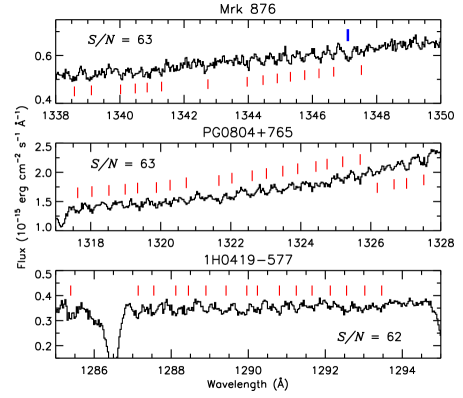
Figure 3: Examples of sawtooth-line MCP Hex fixed pattern noise (FPN) in coadded COS spectra. The red vertical ticks spaced at $\sim$0.4 Å mark the position of Hex FPN. The blue thick tick in the upper panel marks the position of the Milky Way Cl i $\lambda$1347.23. When assumed as a H i Ly$\alpha$, FPN has $\log N_{\mathrm{FPN}}$ $\sim$ 12.5. If a weak IGM H i absorption falls on FPN, the apparent $N_{\mathrm{{\mathrm{H\,\mathsc{i}}}}}$ increases.

2.6 FUSE data

Available FUSE spectra (917–1187 Å) were used to obtain a reliable column density of saturated COS FUV H i Ly$\alpha$ lines, since FUSE spectra cover high-order Lyman lines at $z$ $\leq$ 0.12. The 8th column of Table 3 lists whether the COS AGN has a corresponding FUSE spectrum. The FUSE spectra used in this study are the same ones analysed by Wakker (2006). They are sampled at $\sim$0.0066 Å per pixel, weakly dependent on the wavelength. As they are oversampled, we binned the FUSE spectra by 3, 5 or 7 pixels to increase the S/N. The S/N in general increases toward longer wavelengths, i.e. more reliable Ly$\beta$ profiles than Ly$\gamma$ profiles. The S/N per resolution element at $\sim$1050 Å is listed in parenthesis in the 5th column of Table 3. Since wavelength regions with $S/N$ $<$ 5 are not very useful to deblend saturated lines reliably, we excluded these low-S/N regions in our Lyman series fit. The 4th column in Table 3 accounts for this exclusion. AGN with low-$S/N$ FUSE spectra but with a low-$z$ limit $z$ $\sim$ 0.002 ($\sim$1218 Å) do not have a saturated Ly$\alpha$ (no need for FUSE spectra) or have a higher S/N in FUSE Ly$\beta$ regions of interest than the S/N at $\sim$1050 Å as quoted in Table 3. The resolution varies from AGN to AGN, usually ranging from $\sim$20  km s^-1 above 1000 Å to $\sim$25–30  km s^-1 below 1000 Å. For 3C273, its FUSE observations were taken in the early operation days when the telescope suffered from a focusing problem. This degraded the resolution to $\sim$30  km s^-1 at 1100 Å and to $\sim$60  km s^-1 at 930 Å. The wavelength uncertainty is about 5–10  km s^-1. However, if the Galactic molecular hydrogen with numerous transitions is detected, the wavelength uncertainty can be $\leq$5  km s^-1.

3 Voigt profile fitting analysis

Figure 4: Effect of the S/N on the VPFIT Voigt profile fitting analysis. Left panel: The velocity plot (the relative velocity vs normalised flux) of the $z$ $=$ 0.0030 absorber toward Mrk 876. The velocity centre is set to the redshift of the strongest H i component. The observed spectrum is shown as a black histogram, while the red profile is the generated spectrum using all the fitted components. Blue and magenta profiles with the ticks are the individual fitted components. The top and middle panels show a fiducial 2-component fit and a one-component fit for the COS spectrum, respectively. The bottom panel displays a one-component fit for the STIS E140M spectrum. The noisy STIS spectrum allows a single-component fit with a good $\chi^{2}_{\nu}$, while the higher-S/N COS spectrum requires a two-component fit. The lower part of each panel shows the residual of the fitted components with the normalised $\chi^{2}_{\nu}$. The three numbers in parentheses at the bottom of each panel are the relative velocity in  km s^-1, the $b$ parameter in  km s^-1 and the logarithmic column density, respectively. Right panel: Another absorber at $z$ $=$ 0.0116 toward Mrk 876.

3.1 The Voigt profile fitting analysis

From the profile fitting of identified lines, three line parameters are obtained, the redshift $z$, the column density $N$ in cm^-2 and the line width or the Doppler parameter $b$ in $\textrm{km s}^{-1}$. For thermal broadening, the $b$ parameter ($=\sqrt{2}\sigma$, where $\sigma$ is the standard deviation) is related to the gas temperature $T$ in K by $b$ $=$ $\sqrt{2k_{\mathrm{B}}T/m_{\mathrm{ion}}}$, where $k_{\mathrm{B}}$ is the Boltzmann constant and $m_{\mathrm{ion}}$ is the atomic mass of ions.

We have performed the profile analysis to all the AGN spectra in this study using VPFIT version 10.2 with the VPFIT continuum adjustment option on (Carswell & Webb 2014). We remind readers that the publicly available VPFIT code has been extensively tested by the IGM community over three decades, including comparisons to curve-of-growth fit results. Our already published UVES and HIRES spectra (Kim et al. 2007, 2013, 2016) were also refit with VPFIT v10.2 to be consistent with the new COS and STIS fits. While the new fits overall do not change significantly from the previous ones, the errors produced by VPFIT v10.2 tend to be larger when the components are at absorption wings. Also note that the COS FUV spectra and line lists used in this study are updated from our previous ones analysed in Viel et al. (2017).

Unfortunately, the Voigt profile fitting result is not unique (Kirkman & Tytler 1997; Tripp et al. 2008; Kim et al. 2013). The normalised $\chi^{2}_{\nu}$ criterion does not always guarantee a good actual fit, as illustrated in Fig. 4. The number of fitted components is more sensitive to S/N than the spectral resolution since both STIS and COS spectra resolve the IGM H i lines. As S/N increases, a fitting program often tends to include more narrow, weak components to reproduce small fluctuations. Although additional components added to improve $\chi^{2}_{\nu}$ are in general weak, $\log N_{\mathrm{{\mathrm{H\,\mathsc{i}}}}}\,\leq\!13.5$, an actual change in the fitted parameters depends on S/N and differs for each absorption complex. Despite the non-uniqueness, our fitting analysis uses the same program to fit similar-quality spectra within each data set. Any judgmental calls and systematics would be repeated in similar ways. Therefore, our final combined fitted parameters from different spectrographs can be considered consistent and uniform within our own data sets.

3.2 The COS FUV line spread function

The profile fitting technique requires an instrumental line spread function (LSF) to convolve with the model fit profile. The LSFs of UVES, HIRES, STIS and COS NUV spectra are straightforward and well-characterised (Vogt 1994; Dekker et al. 2000; Riley 2018; Dashtamirova et al. 2019).

The COS FUV LSF is more complicated and changes with wavelength and time. The COS optics do not correct for the mid-frequency wavefront errors due to polishing irregularities in the HST primary and secondary mirrors. This causes the non-Gaussian COS FUV LSF with an extended wing and a broader and shallower core. This is stronger at shorter wavelengths and in particular evident for strong, saturated absorption lines (Kriss 2011; Keeney et al. 2012). The non-Gaussianity produces a broader and shallower line, with the bottom of saturated lines not reaching to a zero flux. Therefore, the flux statistics directly obtained from observed COS spectra cannot be compared with the one from STIS, UVES and HIRES spectra. The non-Gaussian LSF also increases the $N_{\mathrm{{\mathrm{H\,\mathsc{i}}}}}$ detection limit compared to the same Gaussian resolving power.

In addition, the COS FUV detector loses its sensitivity from accumulated exposures known as gain sag. To avoid gain sagged regions, the position of the science spectrum on the FUV detector has been moved to a different Lifetime Position (LP) periodically in the cross-dispersion direction, as noted in the 9th column of Table 3. At the later lifetime positions, the COS FUV LSF has a broader core and more extended non-Gaussian wings (Dashtamirova et al. 2019). Both non-Gaussianity and LP change reduce the resolving power as a function of wavelength and time: at 1300 Å, the resolving power at LP3 decreases $\sim$12% from LP1. Note that $\sim$80% of our COS sample is taken at LP1.

3.3 Voigt profile fitting procedure

Our fitting approach is:

1. The COS FUV/NUV LSF is taken from the HST/COS Spectral Resolution homepage, taking account of the Lifetime Position of the FUV LSF. The STIS E230M LSF is taken from the HST/STIS Spectral Resolution homepage.

2. The error array is scaled to satisfy that the r.m.s. of the unabsorbed region is similar to the average of the errors in the same region, as the rebinning and interpolation during the data reduction often overestimates the error.

3. The appropriate good-fit $\chi^{2}_{\nu}$ is set to be $\sim$1.3, as the average error array does not always correspond to the r.m.s. of the science array and noise is not often Gaussian.

We followed the standard approach for absorption line analysis (Carswell et al. 2002; Kim et al. 2007). First, the entire spectrum was divided into several regions. The number of divided regions is dependent on an apparent underlying continuum shape. When the continuum varies smoothly, divided regions are $\sim$100 Å-long. However, when the continuum varies rapidly such as a region around the Ly$\alpha$ emission or the Ly$\beta$+O vi emission, the length of divided regions is adopted to accommodate the rapid change of the continuum, 5–30 Å. For COS, STIS and FUSE spectra, an initial continuum fit was obtained by iterating a cubic spline polynomial fit for each region, rejecting deviant regions at $|(\mathrm{flux}-\mathrm{fit})/\mathrm{fit}|$ $>$ 0.025 (Songaila 1998). The used fit order is between three and seven, depending on a underlying continuum shape. The continua of each region were joined to form an initial continuum of the entire spectrum. Any disjointed continua at the joined regions are adjusted manually as well as the global continuum after visual inspection, which often gives a better continuum placement. For UVES/HIRES spectra, we used the same normalised spectra analysed by Kim et al. (2013), which follows the same procedure to obtain a localised initial continuum except using the CONTINUUM/ECHELLE command in IRAF.

Second, all possible metal lines were searched for. We started from the most common metals found in the IGM (such as C iv, Si iv and O vi doublets, C ii and Si ii multiplets, and Si iii and C iii singlets) at their expected position for each H i, regardless of $N_{\mathrm{{\mathrm{H\,\mathsc{i}}}}}$. If any of these common metal lines are detected, we searched for other less common metals, such as Fe ii, Mg ii and Al ii. We also used empirically known facts, such as that Mg ii is not associated with low-$N_{\mathrm{{\mathrm{H\,\mathsc{i}}}}}$ lines. When metals were found, they were fit first, using the same $z$ and $b$ values for the same ionic transitions. When metal lines were blended with H i, these H i absorption regions were also included in the fit. The rest of the absorption features were assumed to be H i and were fitted, including all the available higher-order Lyman series, such as Ly$\beta$ and Ly$\gamma$. When $\chi^{2}_{\nu}$ $\geq$ 1.5, additional components are added manually and included only if they improve $\chi^{2}_{\nu}$ significantly. When lines are too narrow to be H i, i.e. $b$ $\leq$ 10  km s^-1, but without a robust line identification, the identification is noted as “??”, but fitted assuming H i. These lines are usually weak at $\log N_{{\mathrm{H\,\mathsc{i}}}}$ $\leq$ 12.8. The contamination by these unidentified metals is negligible at $z$ $<$ 1, but can be around 2–3% at $z$ $\sim$3.

For each fit, we checked whether the initial continuum was appropriate for the available Lyman series and different transitions by the same ion. When necessary, a small amount of continuum adjustment was applied to achieve $\chi^{2}_{\nu}$ $\leq$ 1.3. The entire spectrum was re-fitted with this re-adjusted continuum. In most cases, re-adjusting a local continuum makes it necessary to increase a previous continuum slightly, especially below the Ly$\beta$ emission where weak high-order Lyman absorptions at higher $z$ can depress the continuum. This iteration has been performed several times until the final fit of lines with $\geq$ 3–4$\sigma$ significance was obtained at $\chi^{2}_{\nu}$ $\leq$ 1.3. Due to un-removed fixed pattern noise and continuum uncertainties, we did not fit all the absorption features at $\sim$3.5$\sigma$ such as closely spaced several weak absorption lines as seen in Fig. 3. Any noticeable velocity shifts caused by the COS wavelength calibration uncertainty between the multiple transitions of the same ion are accounted for with the VPFIT “$<$$<$” option. The line identification and/or fitting are independently checked by B. P. Wakker for COS/STIS spectra and R. F. Carswell for STIS/UVES/HIRES spectra, and are finalised by T.-S. Kim.

Since most IGM simulations analyse the Ly$\alpha$ forest without incorporating high-order Lyman series, we also performed a fit using only Ly$\alpha$. Note that even including all the available high-order Lyman lines does not vouch for the completely resolved profile structure of heavily saturated lines at $\log N_{\mathrm{{\mathrm{H\,\mathsc{i}}}}}$ $\geq$ 17–18, if severe line blending and intervening Lyman limits leaves no clean high-order Lyman lines.

The line parameters from VPFIT include the uncertainty due to statistical flux fluctuations and fitting errors. However, they do not include the error due to the continuum placement uncertainty. For the Galactic ISM, the continuum uncertainty is often estimated simply by shifting a fraction of the r.m.s. of the continuum (Savage & Sembach 1991; Sembach et al. 1991) or by estimating all the uncertainties associated with a polynomial function fit to a continuum around an absorption line (Sembach & Savage 1992). In high-$z$ IGM spectra for which VPFIT was initially developed, line blending is too severe to estimate a realistic local continuum around each absorption feature and the flux calibration of high-resolution echelle spectra is not very reliable due to a lack of well-calibrated high-S/N, high-resolution spectra of flux standard stars. The continuum-adjustment $<$$>$ option in VPFIT does not use a similar procedure.

We estimated a continuum error by shifting $\pm$ 0.25$\sigma$ of our fiducial continuum for 50 COS H i absorption features as shown in Fig. 5, since COS IGM H i features are not much affected by line blending. The $\pm$ 0.25$\sigma$ shift is decided by visual inspection (see also Sembach et al. (1991); Penton et al. (2000); Kim et al. (2007)). Obviously the $-$0.25$\sigma$ ($+$0.25$\sigma$) continuum returns a smaller (larger) $b$ and $N_{{\mathrm{H\,\mathsc{i}}}}$. Both sets of line parameters are within the fiducial VPFIT 1$\sigma$ fitting error, with $b$ values being more sensitive to the continuum. In general, the continuum error is $\leq$5% of the fitting error when $\log N_{{\mathrm{H\,\mathsc{i}}}}$ $\geq$ 13.5 and $S/N$ $\geq$ 30 (upper panel). The continuum error becomes larger for low S/N and $N_{{\mathrm{H\,\mathsc{i}}}}$, especially for larger $b$ values. In the lower panel, the continuum error of $b$ and $N_{{\mathrm{H\,\mathsc{i}}}}$ is $\sim$25% for H i with $b$ $\sim$ 40  km s^-1 and $\log N_{{\mathrm{H\,\mathsc{i}}}}$ $\sim$ 13.0 at 1251.4 Å and is $\sim$15% with $b$ $\sim$ 33  km s^-1 and $\log N_{{\mathrm{H\,\mathsc{i}}}}$ $\sim$ 13.0 at 1252.2 Å. We remind that a large fraction of H i at $\log N_{{\mathrm{H\,\mathsc{i}}}}$ $\leq$ 13.1 can be spurious if $S/N$ $\leq$ 20–25.

Although VPFIT does not include a continuum error as in the ISM studies, its fitting errors are calibrated with the curve-of-growth analysis and the associated error array. Weak and broad lines at lower S/N have larger associated error arrays and continuum uncertainties, thus have larger fitting errors. Since our sample has mostly $S/N$ $>$ 20 and our analysed $N_{{\mathrm{H\,\mathsc{i}}}}$ range in the absorption line statistics is $\log N_{{\mathrm{H\,\mathsc{i}}}}$ $\geq$ 13.5, including the continuum fitting error will increase the fiducial fitting error by $\leq$ 5–10%. Our main scientific goal is to quantify the observational estimates as uniformly as possible, reducing a systematic bias. Since it is not clear how to define a reasonable continuum for highly-blended high-$z$ IGM spectra, we therefore used the VPFIT fitting error without including the $\pm$0.25$\sigma$ continuum error in this work for consistency.

A profile fit of a single-line of H i has been claimed to overestimate the true line width by $\sim$1.5 compared to a curve-of-growth fit using all available high-order Lyman lines in STIS, COS and FUSE spectra (Shull et al. 2000; Danforth et al. 2010). We do not find such a tendency when we compare the Ly$\alpha$-only and Lyman series fits for relatively clean, isolated and unsaturated H i Ly$\alpha$ from high-S/N, high-resolution optical UVES/HIRES spectra. Combined with large wavelength calibration uncertainties, imperfect line spread function (LSF) and fixed pattern noise, an observed absorption profile in lower-quality UV spectra does not necessarily show a Voigt-profile shape convolved with the true LSF. We often find that the profile shapes of Lyman lines, such as Ly$\alpha$ and Ly$\beta$ or Ly$\alpha$ and Ly$\gamma$, are inconsistent in COS and FUSE spectra. The discrepancy of $b$ measurements between the profile and curve-of-growth fits is likely to be caused by low-quality data or an inaccurate mathematical treatment in some private profile fitting codes, not by the fundamental inferiority of a profile fit to a curve-of-growth fit. We remind readers that the VPFIT profile fit compromises all the absorption profile shapes included in the fit as a function of S/N. The VPFIT fitting error can be used for reliability of fitted parameters.

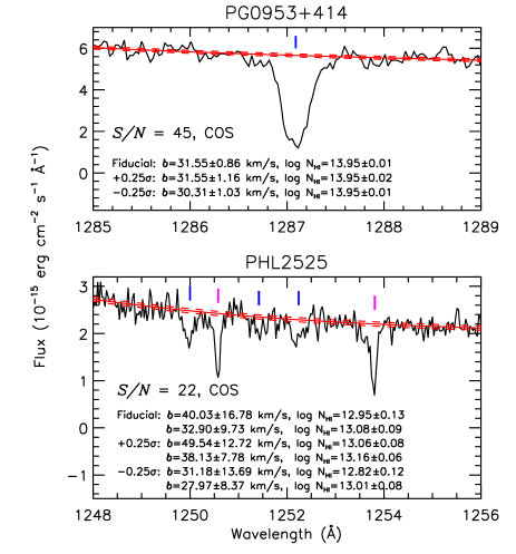
Figure 5: Upper panel: Red solid curve is our final continuum and the red dashed curves are the continuum shifted by $\pm$0.25$\sigma$. The blue vertical tick marks the typical IGM H i lines. The line parameters for each continuum are noted in the panel. Lower panel: Magenta ticks note the Galactic S ii. The first (second) set of line parameters are for the H i line at 1251.4 Å and 1252.2 Å, respectively.

Figure 6: Comparisons of $b$ and $N$ of common H i absorption lines between D16 and our work from the 14 highest-S/N COS AGN (PG 0804+761, 1H 0419–577, PKS 2155–304, TON S210, HE 1228+0131, Mrk 876, IRAS Z06229$-$6434, 3C 273, PG 1116+215, PHL 1811, 1H 0717+714, PG 0953+415, H 1821+643 and PKS 0405–123). The dotted lines delineate the one-to-one correspondence. Upper panels: 136 common H i components with $\log N_{\mathrm{{\mathrm{H\,\mathsc{i}}}}}$ $\in$ [13, 17]. Only components from a similar component structure in both studies are shown. Lower panels: 88 common H i with $\log N_{\mathrm{{\mathrm{H\,\mathsc{i}}}}}$ $\in$ [12.6, 13.0].

Figure 7: Comparisons of $b$ and $N$ of common H i from 30 COS AGN with $S/N\!<\!30$ between D16 and this study. All the symbols are the same as in Fig. 6. Components with $b$ $=$ 100  km s^-1 without errors in D16 indicate highly uncertain. Upper panels: Among our 337 secure H i components, 87% (293/337) shown have a similar component structure. About 6% (19/337) has unaccounted blending by metals or mis-identified as H i in D16. The remaining H i has a different component structure from D16. Lower panels: Out of our 189 secure H i components, 70% (133/189) are common with a similar component structure. About 10% (19/189) suffer from metal contamination or are mis-identified in D16.

3.4 Comparisons with published line parameters

Due to different data treatments and the non-uniqueness of the profile fit, discrepancies between different studies are inevitable. The discrepancy introduces a systematic uncertainty and can result in a contradictory result, especially for low-S/N data. Since only a few sightlines from UVES/HIRES spectra have published line lists besides our own, we compare the fit measurements exclusively using the D16 COS FUV line parameters. D16 sometimes misidentifies the weak Galactic ISM lines such as Mg ii $\lambda\lambda$ 1239.92, 1240.39 and orphaned high-velocity components as intergalactic H i Ly$\alpha$ and does not fully account for contaminations by the ISM lines. Misidentification as metals and unaccounted metal contamination affects $\sim$10% of the D16 lines at their $\log N_{\mathrm{{\mathrm{H\,\mathsc{i}}}}}$ $\in$ [12.6, 17.0]. We use our own line identification and measurements as a reference in this section.

D16 adopts the H i absorption line parameter from a Voigt profile fit at $\log N_{\mathrm{{\mathrm{H\,\mathsc{i}}}}}$ $\leq$ 14 (no other Lyman lines can be detected in low-S/N COS spectra) and a curve-of-growth fit at $\log N_{\mathrm{{\mathrm{H\,\mathsc{i}}}}}$ $\geq$ 14 (high-order Lyman lines can be detected), respectively. Without including FUSE spectra, D16 measures H i line parameters only from a single-line Ly$\alpha$ at $z$ $<$ 0.1. The vast majority ($\sim$86%) of detected IGM H i lines at $z$ $\sim$ 0.15 have $\log N_{\mathrm{{\mathrm{H\,\mathsc{i}}}}}$ $\leq$ 14. Therefore, the comparison is done for our Ly$\alpha$-only fit and their Ly$\alpha$-only profile fit and Ly$\alpha$ curve-of-growth measurements. Both $N$ measurements for a saturated Ly$\alpha$ should be treated as lower limits, although VPFIT gives a very reliable column density for mildly saturated lines.

The two upper panels of Fig. 6 show the comparison of $b$ and $N$ of 136 common H i components for $\log N_{\mathrm{{\mathrm{H\,\mathsc{i}}}}}$ $\in$ [13, 17] from the 14 highest-S/N ($S/N$ $>$ 30) COS AGN analysed by both studies. Only absorption features to have a similar component structure, i.e. a single-component or two-component absorption features, are shown. Among our 173 securely detected H i at $\log N_{{\mathrm{H\,\mathsc{i}}}}$ $\in$ [13, 17], 136 components (79%) have a similar component structure. About 5% (9/173) have unaccounted metal-line blending or are incorrectly identified as H i in D16. For example, an absorption at $\sim$1362.4 Å toward PHL 1811 is identified as H i at $z$ $=$ 0.120700 in D16, but we identify it as Si ii $\lambda$1260.42 at $z$ $=$ 0.08093. The remaining components have a different multi-component structure including saturated absorption complexes or a different line identification from D16. Since both studies do not include a continuum fitting error, the errors are comparable and the VPFIT errors are often larger.

While the column density of common lines is mostly in good agreement, their $b$ shows a larger difference, especially at larger $b$. Twenty components out of 21 with $b$ $>$ 60  km s^-1(12%, 21/173) have $\log N_{\mathrm{{\mathrm{H\,\mathsc{i}}}}}$ $\leq$ 14. At the typical COS S/N in our sample, these broad, weak lines are highly susceptible to the continuum placement and the line alignment among individual extractions to coadd, which reflects in the large $b$ errors. The mean difference and its standard error ($=$ $1\sigma/\sqrt{N}$ with $N$ being the number of common lines) of 173 common H i lines is $\Delta b$ $=$ $0.6\pm 0.4$  km s^-1 and $\Delta\log N_{\mathrm{{\mathrm{H\,\mathsc{i}}}}}$ $=$ $0.03\pm 0.07$. The difference in line parameters for the lines not shown due to a different one-to-one component structure or uncorrected metal blending is obviously much larger.

The difference becomes increasingly larger for 88 common weaker lines at $\log\!N_{\mathrm{{\mathrm{H\,\mathsc{i}}}}}$ $\in$ [12.6, 13.0] (lower panels). As the profile fitting is exclusively based on the absorption profile, the discrepancy is largely due to the difference in the profile shape of weak lines in the two studies, likely caused by the different coaddition procedure and by our improved wavelength re-calibration. As broader lines are highly sensitive to the local S/N and continuum, only 7% (8 out of a total of our 119 secure H i) have $b$ $>$ 60  km s^-1. About 12% (14/119) have unaccounted metal contamination or are wrongly identified as metals in D16. The mean difference and its standard error of common lines is $\Delta b$ $=$ $1.2\pm 0.6$  km s^-1 and $\Delta\log N_{\mathrm{{\mathrm{H\,\mathsc{i}}}}}$ $=$ $0.03\pm 0.01$.

The difference is even larger for lower-S/N spectra (Fig. 7), since the coadded profile shape is more sensitive to the coaddition procedure and line alignment. At $\log N_{\mathrm{{\mathrm{H\,\mathsc{i}}}}}$ $\in$ [13.2, 17.0] ([12.8, 13.2]), the mean difference and its standard error of 293 (133) common lines noted as filled circles is $\Delta b$ $=$ $0.7\pm 0.4$  km s^-1 ($\Delta b$ $=$ $1.2\pm 1.0$  km s^-1) and $\Delta\log N_{\mathrm{{\mathrm{H\,\mathsc{i}}}}}$ $=$ $0.01\pm 0.01$ ($\Delta\log N_{\mathrm{{\mathrm{H\,\mathsc{i}}}}}$ $=$ $0.02\pm 0.01$).

Figure 8 displays the histogram of weak H i components in both studies. With wavelength calibration uncertainties at 5–10  km s^-1 and fixed pattern noise (FPN), the fitted line parameters, in particular $b$, and identifications of weak lines are not as reliable as for strong lines. We measured 580 components at $\log N_{\mathrm{{\mathrm{H\,\mathsc{i}}}}}$ $\leq$ 13.2. Certain and uncertain ($\sim$3.5$\sigma$) components are 73% (422/580) and 25% (146/580), respectively. The remaining is FPN features (gray-shade histogram, Fig. 3). Real weak absorption features can be missed easily in noisy spectra and a large fraction of detected weak lines can be spurious at $\log N_{\mathrm{{\mathrm{H\,\mathsc{i}}}}}$ $\leq$ 12.8. This incompleteness decreases the number of detected H i lines toward lower-$N_{{\mathrm{H\,\mathsc{i}}}}$ end. We did not attempt to remove any FPN in our coadding procedure (Wakker et al. 2015). With a very conservative approach, we flagged weak absorption features in coadded spectra as FPN only when we were certain by examining individual extractions. Not all of flagged fixed pattern noise were fitted.

In the lower panel of Fig. 8, the distribution of their 576 H i components and 468 FPN features from D16 suggests that FPN features become dominant at $\log N_{\mathrm{{\mathrm{H\,\mathsc{i}}}}}$ $\leq$ 12.8. D16 strictly measures all the absorption features at $\geq$3$\sigma$, thus their detection of weak absorption features is likely to be more objective and less biased. About 61% (287/468) of absorption features flagged as FPN in D16 are not measured in our study. However, their identification of weak lines should be taken with caution. For example, their H i features at $\sim$1288 Å toward HE 1228+0131 (their Q 1230+0115) and at $\sim$1292 Å toward 1H 0419$-$577 (their RBS 542) are likely to be FPN as shown in Fig. 3.

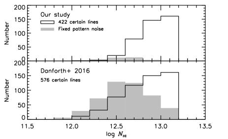
Figure 8: Histograms of $N_{{\mathrm{H\,\mathsc{i}}}}$ of weak H i from the 44 COS AGN in common. The number distribution of H i clearly shows a turnover at $\log N_{\mathrm{{\mathrm{H\,\mathsc{i}}}}}$ $\leq$ 13 due to missed detections by noise.

4 Transmitted H i flux statistics

4.1 The mean flux and the flux PDF

The two simplest measurements of the amount of intergalactic H i are the transmitted mean flux and the transmitted flux probability distribution function (PDF). Both measurements are motivated by the current picture of the IGM in which the absorption arises from continuous matter fluctuations instead of discrete clouds, so are measured from the continuous spectrum and often referred to as “continuous flux statistics”.

The mean H i flux is the average intervening absorption along the sightline and is proportional to the mean $N_{\mathrm{{\mathrm{H\,\mathsc{i}}}}}$ through a combination of the gas density, the number of lines and line widths in redshift space. For the highly photoionised IGM, $N_{\mathrm{{\mathrm{H\,\mathsc{i}}}}}$ is inversely proportional to the UV background intensity. In practice, the mean flux is used to calibrate simulations to observations and constrains the combined effect of the baryon density, the amplitude of the matter density fluctuation $\sigma_{\mathrm{8}}$, the temperature-density relation and the UVB (Rauch et al. 1997; Kirkman et al. 2007; Becker et al. 2013; Oñorbe et al. 2017).

The mean H i flux is related to the effective opacity $\tau_{\mathrm{eff}}$,

$$<\!F\!>\,=\,<\!f_{\mathrm{obs}}/f_{\mathrm{cont}}\!>\,=\,<\!e^{-\tau}\!>\,=e^{-\tau_{\mathrm{eff}}},$$ (2)

where $f_{\mathrm{obs}}$ is the observed flux, $f_{\mathrm{cont}}$ is the continuum flux, $\tau$ is the optical depth and $\tau_{\mathrm{eff}}$ is the effective optical depth. The effective optical depth is introduced to account for the fact that when close to 0 the normalised flux cannot be converted to the correct $\tau$. The uncertainty is largely due to the continuum placement and the amount of unremoved metal lines, but this is not straightforward to determine. Based on a visual inspection of each spectrum, we arbitrarlly define the error as 0.25 times the r.m.s. of the unabsorbed region.

The probability distribution function (PDF or $P(F)$) of the transmitted flux $F$ is a higher order continuous statistic. It is defined as the fraction of pixels having a flux between $F$ and $F$ $+$ $\Delta F$ for a given flux $F$ (Jenkins & Ostriker 1991; Rauch et al. 1997; McDonald et al. 2000). While the mean H i flux is a one-parameter function of $z$, the flux PDF is a two-parameter function that constrains the amount of absorptions as a function of $z$ and absorption strength $F$. Being a higher-order statistic, the PDF is more sensitive to the profile shape of absorption lines through the density distribution and thermal state of the IGM than the mean H i flux (Bolton et al. 2008). In practice, the PDF is also sensitive to the continuum uncertainties at $F$ $\sim$ 1 and to the amount of unremoved metal lines at $F$ $\sim$ 0.4 (Kim et al. 2007; Calura et al. 2012; Lee 2012; Rollinde et al. 2013).

With a large number of pixels per redshift bin, the conventional standard deviation significantly underestimates the actual PDF errors. Therefore, the errors were calculated using a modified jackknife method as outlined in Lidz et al. (2006). First, all the individual spectra longer than 50 Å in each $z$ bin are put together to generate a single, long spectrum to calculate the averaged PDF, with the bin size $\Delta F$ $=$ 0.05 at 0 $<$ $F$ $<$ 1. Pixels with $F$ $\leq$ 0.025 or $F$ $\geq$ 0.975 are included in the $F$ $=$ 0.0 and the $F$ $=$ 1.0 bins. Second, this long spectrum was divided into $n_{c}$ chunks with a length of $\sim$50 Å. In the $\tilde{z}\!=\!0.08$ bin, $n_{c}$ is 40 from the single long spectrum composed from 24 individual spectra. If the PDF estimated at the flux bin $F_{i}$ is $\widehat{P}(F_{i})$ and the PDF estimated without the $k$-th chunk at the flux bin $F_{i}$ is $\widetilde{P}_{k}(F_{i})$, then the variance at a flux bin $F_{i}$ becomes

$$\sigma_{i}^{2}=\sum_{k=1}^{n_{c}}[\widehat{P}(F_{i})-\widetilde{P}_{k}(F_{i})]^{2}.$$ (3)

This modified jackknife method is not sensitive to the length of chunks, but the errors become larger when the number of chunks is too small.

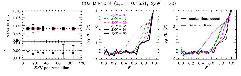
Figure 9: The effect of S/N and undetected weak lines on the flux statistics. The metal-free spectrum of Mrk 1014 (COS FUV AGN) was generated from the detected lines, assuming the Gaussian LSF of 19  km s^-1. We also added the several, different artificial Gaussian noise and/or supposedly undetected weak lines at $\log N_{\mathrm{{\mathrm{H\,\mathsc{i}}}}}$ $\in$ [12.3, 13.0]. Left panel: The mean H i flux (filled circles) does not change with S/N. Undetected weak lines due to a low S/N (open red squares without errors for clarity) do not have any noticeable effect seen from $\Delta\!=\!\bar{F}_{\mathrm{weak\,lines}}\!-\!\bar{F}$ in the lower panel. Middle panel: The flux PDF converges at $0.1\!<\!F\!<\!0.7$ if $S/N\!>\!23$. Right panel: The PDFs including artificially added undetected weak lines (thicker curves) are indistinguishable from the PDFs from detected H i at $\log N_{\mathrm{{\mathrm{H\,\mathsc{i}}}}}\!\geq\!13$ (thin curves). The black curves are for $S/N\!=\!68$, while the colour at other S/N is the same as used in the middle panel.

4.2 Data quality on the flux statistics

Removing the metal contamination in the AGN spectrum is not straightforward, especially when metals can be often blended with strong H i complexes over a considerable wavelength range. In addition, due to the non-Gaussian LSF of COS and STIS, the flux statistics directly measured from these spectra cannot be compared to the UVES/HIRES spectra (see Section 3.2).

To avoid these drawbacks, a set of H i-only spectra was generated for each AGN. We included the fitted H i only with $\log N_{\mathrm{{\mathrm{H\,\mathsc{i}}}}}$ $<$ 19, excluding sub-DLAs. A Gaussian LSF was assumed to be 19  km s^-1, 12  km s^-1, 10  km s^-1 and 6.7  km s^-1  for COS FUV, COS NUV, STIS and UVES/HIRES data, respectively. Note that the majority of our COS FUV spectra were taken at Lifetime Position 1 when the approximated Gaussian resolution was $\sim$19  km s^-1. As almost all COS H i lines are resolved, accounting for a degraded resolution by a few km/sec at a later Lifetime Position does not make any difference in the generated spectrum. The wavelength coverage used for the Ly$\alpha$-only fit is in general larger than for the Lyman series fit, while both fits reproduce the observed absorption profiles within noise. Therefore, we used the Ly$\alpha$-only fit to generate the metal-free spectrum to study the flux statistics. Lowest $N_{\mathrm{{\mathrm{H\,\mathsc{i}}}}}$ included differs for each AGN. We also added artificial Gaussian noise to each generated spectrum, using the observed S/N ($S/N$ $=$ $1/\sigma$, where 1$\sigma$ is the r.m.s. of the unabsorbed region).

The effect of different S/N and undetected weak lines on the continuous flux statistics is demonstrated in Fig. 9. In the left panel, the filled circles are $<$$F$$>$ measured from the generated spectrum of Mrk 1014 as a function of artificially added S/N. The mean flux is not sensitive to S/N as expected from Gaussian noise being symmetrical at $F$ $=$ 1, although the errors (0.25 times the r.m.s. of the unabsorbed region) are larger at lower S/N by definition.

Mrk 1014 is one of the lowest-S/N COS FUV spectra in this study with a detection limit $\log N_{\mathrm{{\mathrm{H\,\mathsc{i}}}}}$ $\sim$ 13.0. However, the highest-S/N COS FUV spectra (3C 273 and Mrk 876) show H i at $\log N_{\mathrm{{\mathrm{H\,\mathsc{i}}}}}$ $<$ 13.0, indicating that real weak absorptions are undetected in low-S/N spectra. We manually add the expected number of H i lines at $\log N_{\mathrm{{\mathrm{H\,\mathsc{i}}}}}$ $\in$ [12.3, 13.0] by extrapolating from the number of lines at $N_{\mathrm{{\mathrm{H\,\mathsc{i}}}}}$ $>$ 13.0 per $N_{\mathrm{{\mathrm{H\,\mathsc{i}}}}}$ (Section 5.1 for details). The red open squares are the mean H i flux averaged from 10 generated spectra including artificial weak lines at each S/N. Added weak lines produce more absorption, but $<$$F$$>$ decreases insignificantly by $\sim$0.004, less than 0.5%. The expected decrease becomes even lower for higher-S/N sightlines since they have a lower $N_{\mathrm{{\mathrm{H\,\mathsc{i}}}}}$ detection limit so that the number of added weak lines below the detection limit down to $\log N_{\mathrm{{\mathrm{H\,\mathsc{i}}}}}$ $\sim$ 12.3 is smaller. We conclude that undetected weak lines do not have any meaningful impact on the mean H i flux.

The S/N has a significant impact on the PDF, as shown in the middle panel of Fig. 9. The PDF at 0.1 $<$ $F$ $<$ 0.7 converges if $S/N$ $>$ 23. In the right panel, adding supposedly undetected weak lines has a noticeable impact on the PDF only when $S/N$ $>$ 60 at $F$ $\geq$ 0.85 since added weak lines with $\log N_{\mathrm{{\mathrm{H\,\mathsc{i}}}}}$ $\leq$ 13.0 ($F$ $\geq$ 0.9) can be detected only at high S/N. Note that this discrepancy is negligible for COS FUV spectra with observed $S/N$ $>$ 60, since H i at $\log N_{\mathrm{{\mathrm{H\,\mathsc{i}}}}}$ $\in$ [12.5, 13.0] is detected and included in the PDF at $F$ $\geq$ 0.9.

The PDF at $F$ $\sim$ 1 is also subject to continuum placement uncertainty, especially at high redshifts (Kim et al. 1997; Calura et al. 2012; Lee 2012). The largest systematic uncertainty comes from the unknown, possible overall continuum depression by the Gunn-Peterson effect (Faucher-Giguére et al. 2008a), which is likely to be removed during the local continuum fit as we did. At $z_{\mathrm{em}}$ $<$ 3.5–3.7, the profile fit using all the available Lyman lines of the highest-S/N QSO spectra does not require a significant Gunn-Peterson depression (Calura et al. 2012). Our previous work (Kim et al. 2007, their Fig. 2) and our experience on high-S/N UVES/HIRES QSO spectra suggest that a continuum in general changes very smoothly over large wavelength ranges. Therefore, we do not expect our continuum error is much larger than $\sim$2% at $z$ $\sim$ 3 if the S/N is larger than $\sim$70 per resolution element. Note that 21 out of our 24 UVES/HIRES QSO spectra have $S/N$ $\geq$ 70. Since we apply the same procedure to the continuum placement for our high-$z$ QSO spectra, we assume that a systematic continuum uncertainty is smaller than the statistical uncertainty at $z$ $<$ 3.5.

Our approach directly removes the metal contribution from the IGM, instead of commonly-used masking the metal regions (McDonald et al. 2001; Kirkman et al. 2007) or removing statistically using the metal contribution above the Ly$\alpha$ emission (Faucher-Giguére et al. 2008a). At $z$ $<$ 0.5, metals are almost fully identified, as line blending is low and the Ly$\alpha$ line is observed down to $z$ $=$ 0 so that associated metals are easily identified. At $z$ $>$ 1, most medium-strength/strong metal lines are fully identified, however, weak narrow lines are not. Fortunately, when medium-strength/weak unidentified metal lines are blended with H i lines, their contribution to the whole blended profile is often negligible. We empirically conclude that the unremoved metal contamination contributes $\leq$1% to $<$$F$$>$ at $z$ $\sim$ 3 and only affect the PDF at $F$ $\sim$ 1.

The PDF from most COS FUV and STIS spectra (S/N $\sim$ 18–40) is sensitive to the continuum placement at $F$ $\sim$ 1 and to S/N at $F$ $>$ 0.7, and the PDF from most UVES/HIRES spectra (S/N $\geq\!60$) has the largest uncertainty at $F$ $\sim$ 1 due to the continuum error. Out of five COS NUV spectra, only one (HE 1211–1322) has a lower S/N (10–15) than the S/N cut of 18 for COS FUV data. However, its contribution to the total wavelength length at $z$ $\sim$ 1 is only 18%. Therefore, we will consider the PDF only at 0.1 $<$ $F$ $<$ 0.7 at 0 $<$ $z$ $<$ 3.6 in this study.

4.3 The observed mean H i flux

Table 4: Averaged mean H i flux $<$$F$$>_{\mathrm{ave}}$

$\tilde{z}$	$z$ range	# of AGN	$<$$F$$>_{\mathrm{ave}}{\bf{}^{\mathrm{a}}}$
0.08	0.00–0.15	40	0.983$\pm$0.003$\pm$0.006
0.25	0.15–0.45	24	0.978$\pm$0.002$\pm$0.005
0.98	0.78–1.29	5	0.943$\pm$0.006$\pm$0.010
2.07	1.85–2.30	17	0.872$\pm$0.013$\pm$0.001
2.54	2.30–2.80	12	0.790$\pm$0.014$\pm$0.001
2.99	2.80–3.20	6	0.719$\pm$0.017$\pm$0.001
3.38	3.20–3.55	2	0.642$\pm$0.016$\pm$0.001

Notes – a: The first error is the jackknife error of individual $<$$F$$>$ values and the second error is the standard deviation of their adopted associated error (0.25$\sigma$).

The upper panel of Fig. 10 plots the mean H i flux of individual AGN from the Ly$\alpha$-only fit as a function of $\log(1$ $+$ $z)$ with gray filled circles. The mean flux toward each sightline is available as an online table on the MNRAS website (Table S1). The adopted error of 0.25$\sigma$ of unabsorbed regions does not reflect a true relative error, but the S/N of each spectrum, and this adopted error is likely to be over-estimated. The filled circles are the averaged mean H i flux $<$$F$$>_{\mathrm{ave}}$, listed in Table 4. This is not an arithmetic mean of individual $<$$F$$>$ at each $z$ bin, but is estimated from a single long spectrum combined from all the generated H i-only spectra with an appropriate Gaussian noise. Due to a large number of pixels in each $z$ bin, any standard error estimates significantly under-estimate a true error. Therefore, we used the sum of the two error estimates: the jackknife error of individual $<$$F$$>$ values in the $z$ bin and the standard deviation of the associated error (0.25$\sigma$) of individual $<$$F$$>$ to account for a continuum uncertainty. Our measurement is consistent with the previous observations within the errors.

The mean flux from each sightline shows a large scatter (the inset plot). This scatter is more clearly seen in the lower panel. The deviation from the averaged mean flux at each sightline is calculated using the standard error ($1\sigma_{<F>}$ $=$ $1\sigma/\sqrt{N}$ with $N$ being the number of sightlines) of the arithmetic mean of all the sightlines within a given redshift range $\Delta z$, but excluding the sightline in consideration. Due to the paucity of data points at higher redshifts, we use a different $\Delta z$ at different redshifts: $\Delta z$ $=$ 0.05 at $z$ $<$ 0.45, $\Delta z$ $=$ 0.51 at $z$ $\sim$ 1, $\Delta z$ $=$ 0.2 at 1.9 $<$ $z$ $<$ 3.0 and $\Delta z$ $=$ 0.35 at 3.0 $<$ $z$ $<$ 3.6, respectively. About 71% of the sightlines have a mean flux at $\geq$1$\sigma_{<F>}$ and about 55% have a mean flux at $\geq$2$\sigma_{<F>}$. This considerable cosmic variance depends largely on the occurrence rate of passing through intervening overdense or underdense environments such as galaxy groups or galaxy voids. Note that the large discrepancy from the Becker measurement noted as the cyan cross (Becker et al. 2013) is mainly caused by the fact that our sample does not have enough sightlines at $z$ $>$ 3, given that the cosmic variance is important.

The overlaid solid black curve is a conventional single power-law fit to individual measurements at 0 $<$ $z$ $<$ 3.6, $\ln<$$F$$>$ $=$ $-\tau_{\mathrm{eff}}$ $=$ $A_{0}(1+z)^{\alpha}$ with $A_{0}$ $=$ $-0.0060\pm 0.0001$ and $\alpha$ $=$ $2.87\pm 0.01$. Note that we used a median error $\pm$0.005 of the UVES/HIRES data as the error of both COS/STIS individual $<$$F$$>$ for this fit, since the adopted error of the latter incorrectly gives more weight to the UVES/HIRES data at $z$ $>$ 1.5. This simple single power law over-predicts $<$$F$$>$ at $z$ $<$ 1.5, i.e. less absorption than the observations. The suggested single exponential fit (red curve) by Oñorbe et al. (2017) also overpredicts the observations at $z$ $<$ 1.5, more than a simple power law.

In fact, $<$$F$$>$ increases faster (less absorption) from $z$ $=$ 3.6 $\rightarrow$ 1.5, slows down at $z$ $\sim$ 1, then becomes almost invariant at $z$ $<$ 0.5. This requires a more complicated fitting function. If a double power law to individual data points is assumed, $A_{0}$ $=$ $-0.0145\pm 0.0003$ and $\alpha$ $=$ $1.86\pm 0.07$ at $z$ $<$ 1.5 (magenta dashed curve) and $A_{0}$ $=$ $-0.0040\pm 0.0001$ and $\alpha$ $=$ $3.18\pm 0.02$ at $z$ $>$ 1.5 (orange dashed curve), respectively. Note that a single power-law fit at $z$ $<$ 0.5 is similar to the fit at $z$ $<$ 1.5: $A_{0}$ $=$ $-0.0142\pm 0.0004$ and $\alpha$ $=$ $2.06\pm 0.16$ (not shown). This means that the mean flux does not show any abrupt evolutionary change at $z$ $<$ 1.5.

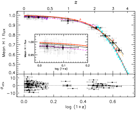
Figure 10: Upper panel: The mean H i flux as a function of $z$ (upper x-axis) and $\log(1$ $+$ $z)$ (lower x-axis) is plotted as gray filled circles for individual sightlines and as filled circles for the averaged mean flux for each $z$ bin. The x-axis error is the $z$ range. The y-axis error is the 0.25 r.m.s. of unabsorbed regions for individual sightlines and is the sum of the jackknife error and standard deviation of the errors of individual $<$$F$$>$ in each bin for the averaged mean flux. The inset plot shows the sightline variation at low $z$ more clearly. In both panels, the solid curve is a single power-law model for our individual measurements at 0 $<$ $z$ $<$ 3.6, while the magenta and orange dashed curves are the fit for $z$ $<$ 1.5 and $z$ $>$ 1.5, respectively. The red curve is the single exponential fit $\tau$ $=$ $0.00126\times e^{(3.294\times\sqrt{z})}$ suggested by Oñorbe et al. (2017). The dark-orange triangles, upside-down purple triangles and cyan crosses are taken from Kirkman et al. (2007), Danforth et al. (2016) and Becker et al. (2013), respectively. Lower panel: Deviation of the individual mean flux from $<$$F$$>_{\mathrm{ave}}$.

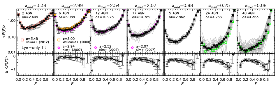
Figure 11: Upper panel: The observed mean PDF $<$$P(F)$$>$ as a function of $F$ with the filled circles. The overlaid thin gray curves are the PDF of individual AGN. The x-axis error shows the $F$ bin size of 0.05, while the y-axis error is from the modified jackknife method. The green open squares at $z$ $\sim$ 0.08 and 0.25 are $<$$P(F)$$>$ measured from a subset of 14 ($\Delta X$ $=$ 1.467) and 4 ($\Delta X$ $=$ 0.414) high-S/N COS spectra with $S/N$ $\geq$ 30. The absorption path length from the subset is only 30% and 10%, which leads to the spiky $<$$P(F)$$>$ as a function of $F$. In the $\tilde{z}$ $=$ 2.54 and 2.07 panels, our new measurements (filled circles) are indistinguishable from our previous ones (open magenta diamonds, Kim et al. (2007)). Lower panel: The difference between the mean PDF at $\tilde{z}$ $=$ 3.38 and at the given redshift.

4.4 The observed flux PDF

The upper panel of Fig. 11 shows the mean PDF, $<$$P(F)$$>$, measured from a single, long spectrum combined from all the H i-only AGN spectra as filled circles at each $z$ bin. Table 5 lists $<$$P(F)$$>$ and their errors estimated from the modified jackknife method. The absorption path length $\Delta X$ noted in each panel provides a relative sample size, as the number of included pixels is meaningless due to the different pixel size for the different data sets. The green open squares at $z$ $\sim$ 0.08 and 0.25 are from a subset of high-S/N COS spectra. A factor of 10 smaller $\Delta X$ at $z$ $\sim$ 0.25 causes $<$$P(F)$$>$ from the subset sample to be $\sim$25% smaller, demonstrating importance of a large sample to reduce systematic bias.

At the redshift bin with a large number of AGN, the individual PDF (thin gray curves) varies significantly, 40–50% at $F$ $\sim$ 0.5. This sightline variance becomes stronger at lower redshifts. This is in part caused by the fact that the number of pixels per sightline is on average a factor of 18 smaller at $z$ $<$ 0.5 than at $z$ $>$ 2.5, i.e. coverage bias, and in part by the fact that the forest clustering increases at lower redshifts (Kim et al. 1997).

In the $\tilde{z}$ $=$ 3.38 panel, a noticeable difference exists between the PDF measured by Calura et al. (2012) (open dark-orange squares) and our measurements at $F$ $>$ 0.5. Although within 1$\sigma$ errors, the amount of difference depends on $F$, suggesting that the main cause of the discrepancy might be the continuum uncertainties at high redshifts (Calura et al. 2012), in addition to the small number of sightlines included in both studies and the different redshift range studied. In the $\tilde{z}$ $=$ 2.99 panel, the open orange squares are the PDF at $z$ $=$ 3.0 measured by McDonald et al. (2000), about 1.7$\sigma$ larger than our present measurements. The discrepancy is in part caused by their imperfect metal removal as metal contamination increases $<$$P(F)$$>$ especially at 0.2 $<$ $F$ $<$ 0.6 (Kim et al. 2007), and in part by the sightline variance as their sample size is smaller by a factor of 2. In the same panel, the open purple triangles are our previous measurement at $z$ $=$ 2.94 which are $\sim$1.4$\sigma$ smaller (Kim et al. 2007). Since we treated the data in a similar manner in both studies, the discrepancy is likely due to the fact that our older sample size is 2 times smaller and the measurement was done at a slightly lower $z$.

At each $z$, the overall shape of $<$$P(F)$$>$ is a convex function with the $z$-independent minimum at $F$ $\sim$ 0.2: $<$$P(F)$$>$ rapidly decreases at $F$ $=$ 0.0 $\rightarrow$ 0.2, then it increases slowly at $F$ $=$ 0.2 $\rightarrow$ 0.6 and rapidly at $F$ $=$ 0.6 $\rightarrow$ 1.0. At a given $F$, $<$$P(F)$$>$ decreases rapidly as $z$ decreases (the lower panel), consistent with the higher mean flux (lower H i absorption) at lower $z$. If the line width of a typical H i line is assumed to be $b$ $\sim$ 25  km s^-1, $F$ $=$ 0.3 ($F$ $=$ 0.7) corresponds to $\log N_{\mathrm{{\mathrm{H\,\mathsc{i}}}}}$ $\sim$ 13.7 (13.1). This approximately translates that only lines with $\log N_{\mathrm{{\mathrm{H\,\mathsc{i}}}}}$ $\geq$ 13.7 can contribute to the PDF at $F$ $\sim$ 0.3. If we ignore the $b$-dependence on $z$ and $N_{\mathrm{{\mathrm{H\,\mathsc{i}}}}}$, a factor of 18 lower $<$$P(F$ $=$ $0.3)$$>$ at $\tilde{z}$ $=$ 0.08 than at $z$ $\sim$ 3.37 indicates that the number of H i absorbers with $\log N_{\mathrm{{\mathrm{H\,\mathsc{i}}}}}$ $\geq$ 13.7 is a factor of 18 lower at $\tilde{z}$ $=$ 0.08.

Table 5: Averaged H i PDF from the Ly$\alpha$-only fit

$F$	$\tilde{z}$ $=$ 0.08	$\tilde{z}$ $=$ 0.25	$\tilde{z}$ $=$ 0.98	$\tilde{z}$ $=$ 2.07	$\tilde{z}$ $=$ 2.54	$\tilde{z}$ $=$ 2.99	$\tilde{z}$ $=$ 3.38
	$z$ $=$ 0.00–0.15	$z$ $=$ 0.15–0.45	$z$ $=$ 0.78–1.29	$z$ $=$ 1.85–2.30	$z$ $=$ 2.30–2.80	$z$ $=$ 2.80–3.20	$z$ $=$ 3.20–3.55
0.00	0.039$\pm$0.009	0.042$\pm$0.011	0.225$\pm$0.063	0.493$\pm$0.074	1.024$\pm$0.646	1.729$\pm$0.930	2.152$\pm$0.609
0.05	0.022$\pm$0.007	0.026$\pm$0.007	0.107$\pm$0.029	0.207$\pm$0.028	0.383$\pm$0.094	0.471$\pm$0.274	0.721$\pm$0.187
0.10	0.018$\pm$0.006	0.024$\pm$0.005	0.067$\pm$0.017	0.129$\pm$0.021	0.244$\pm$0.074	0.286$\pm$0.124	0.445$\pm$0.123
0.15	0.015$\pm$0.007	0.019$\pm$0.004	0.061$\pm$0.015	0.128$\pm$0.026	0.207$\pm$0.056	0.285$\pm$0.107	0.359$\pm$0.096
0.20	0.014$\pm$0.003	0.020$\pm$0.004	0.059$\pm$0.014	0.125$\pm$0.026	0.193$\pm$0.059	0.256$\pm$0.086	0.310$\pm$0.085
0.25	0.015$\pm$0.003	0.019$\pm$0.003	0.049$\pm$0.013	0.115$\pm$0.023	0.207$\pm$0.041	0.243$\pm$0.091	0.359$\pm$0.096
0.30	0.019$\pm$0.005	0.023$\pm$0.004	0.050$\pm$0.013	0.119$\pm$0.020	0.203$\pm$0.044	0.256$\pm$0.109	0.328$\pm$0.107
0.35	0.019$\pm$0.004	0.029$\pm$0.006	0.051$\pm$0.013	0.128$\pm$0.026	0.198$\pm$0.041	0.266$\pm$0.098	0.367$\pm$0.112
0.40	0.021$\pm$0.005	0.026$\pm$0.005	0.060$\pm$0.015	0.138$\pm$0.033	0.218$\pm$0.047	0.284$\pm$0.115	0.411$\pm$0.142
0.45	0.025$\pm$0.008	0.029$\pm$0.006	0.064$\pm$0.015	0.151$\pm$0.031	0.250$\pm$0.044	0.281$\pm$0.110	0.394$\pm$0.122
0.50	0.029$\pm$0.007	0.039$\pm$0.008	0.084$\pm$0.020	0.177$\pm$0.036	0.281$\pm$0.058	0.312$\pm$0.128	0.444$\pm$0.142
0.55	0.033$\pm$0.008	0.044$\pm$0.010	0.105$\pm$0.026	0.189$\pm$0.035	0.307$\pm$0.061	0.379$\pm$0.139	0.504$\pm$0.172
0.60	0.040$\pm$0.020	0.054$\pm$0.010	0.109$\pm$0.024	0.216$\pm$0.049	0.361$\pm$0.083	0.459$\pm$0.158	0.543$\pm$0.176
0.65	0.046$\pm$0.011	0.074$\pm$0.011	0.151$\pm$0.035	0.265$\pm$0.043	0.386$\pm$0.092	0.530$\pm$0.177	0.654$\pm$0.210
0.70	0.063$\pm$0.015	0.092$\pm$0.015	0.202$\pm$0.047	0.316$\pm$0.050	0.451$\pm$0.121	0.644$\pm$0.166	0.763$\pm$0.220
0.75	0.102$\pm$0.022	0.157$\pm$0.023	0.359$\pm$0.079	0.403$\pm$0.070	0.586$\pm$0.120	0.740$\pm$0.185	0.926$\pm$0.275
0.80	0.220$\pm$0.055	0.351$\pm$0.052	0.565$\pm$0.120	0.568$\pm$0.101	0.825$\pm$0.183	0.999$\pm$0.291	1.234$\pm$0.359
0.85	0.540$\pm$0.092	0.851$\pm$0.123	1.132$\pm$0.236	0.827$\pm$0.151	1.199$\pm$0.216	1.397$\pm$0.373	1.620$\pm$0.506
0.90	1.533$\pm$0.246	2.043$\pm$0.285	2.078$\pm$0.426	1.595$\pm$0.335	1.977$\pm$0.450	2.118$\pm$0.623	1.928$\pm$0.622
0.95	4.123$\pm$0.852	4.049$\pm$0.544	3.685$\pm$0.746	4.216$\pm$0.819	4.007$\pm$0.834	3.463$\pm$0.955	2.670$\pm$0.948
1.00	13.066$\pm$2.807	11.988$\pm$1.628	10.738$\pm$2.208	9.494$\pm$2.014	6.494$\pm$1.117	4.601$\pm$1.099	2.870$\pm$1.145

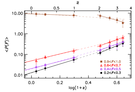
Figure 12: The redshift evolution of $<$$P(F)$$>$ at the larger $F$ bin size of 0.1. The $F$ $=$ 0.95 bin is included only for a qualitative comparison.

The $z$-evolution of the PDF is more clearly illustrated in Fig. 12 with a larger $F$ bin size $\Delta F$ $=$ 0.1 to decrease a statistical fluctuation caused by a smaller $F$ range. The overlaid dashed line is a single power-law fit $P(F,z)$ $=$ $C_{0}(1$ $+$ $z)^{C_{1}}$ at 0 $<$ $z$ $<$ 3.6, while the solid line is a double power-law fit at $z$ $<$ 1.5 and $z$ $>$ 1.5, respectively, with the fit parameters listed in online Table S2 on the MNRAS web site.

This evolution reflects the fact that Ly$\alpha$ forest absorption typically probes rarer, higher density gas toward lower redshift due to the evolution of the UVB and the decrease in the proper density of gas in the IGM (Khaire & Srianand 2019). Although a different IGM structure corresponds to a different $F$ (or $N_{\mathrm{{\mathrm{H\,\mathsc{i}}}}}$) at a different $z$ due to large-scale structure evolution (Davé et al. 1999; Schaye 2001; Hiss et al. 2018), the pixels with 0.2 $<$ $F$ $<$ 0.7 and $F$ $\sim$ 1 can be considered to sample roughly the filaments/sheets and cosmic flux voids (under-dense regions and regions under enhanced ionisation radiation) of the low-density IGM structure, respectively. The $<$$P(F,z)$$>$ measurements shown in Fig. 12 qualitatively suggest that the volume fraction of flux voids increases rapidly from $z$ $\sim$ 3.5 down to $z$ $\sim$ 1.5, reflecting the higher Hubble expansion rate and also probably the rapidly increasing number of UV H i ionising photons compared to lower redshifts (Theuns et al. 1998a; Davé et al. 1999; Haardt & Madau 2012). The volume fraction increases slowly at $z$ $<$ 1.5. In contrast, the volume fraction occupied by IGM filaments and sheets decreases continuously with time, faster at $z$ $>$ 1.5 and slower at $z$ $<$ 1.5.

5 Absorption line statistics

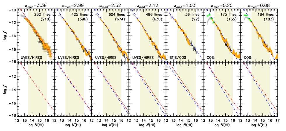
Figure 13: Upper panel: The logarithmic CDDF ($\log f$) as a function of $\log N_{\mathrm{{\mathrm{H\,\mathsc{i}}}}}$. The orange and black dots are the CDDF measured from the Lyman series and the Ly$\alpha$-only fits above the detection limit for each $z$ bin, while gray dots are measured from the Lyman series fit below the detection limit. The filled green circles at $\tilde{z}\!=\!0.08$ and $\tilde{z}\!=\!0.25$ plot the CDDF at $\log N_{\mathrm{{\mathrm{H\,\mathsc{i}}}}}$ $\leq$ 13.5 measured from a subset of the high-S/N COS spectra used in Fig. 11, clearly demonstrating the impact of incompleteness. For clarity, the Poisson errors are shown only in the $\tilde{z}$ $=$ 3.38 panel for selected data points. In the upper right corner the first (second) value is the number of lines at $\log N_{\mathrm{{\mathrm{H\,\mathsc{i}}}}}$ $\in$ [13.5, 16.0] from the Lyman series (Ly$\alpha$-only) fit. The red dot-dashed line on the $\tilde{z}$ $=$ 3.38 panel the is a power-law fit to the lines from the Lyman series fit at $\log N_{\mathrm{{\mathrm{H\,\mathsc{i}}}}}$ $\in$ [13.5, 16.0] (beige shaded regions), while the blue dashed line on every panel is a power-law at the given $z$ for the Lyman-series-fit lines over the same $N_{\mathrm{{\mathrm{H\,\mathsc{i}}}}}$ range. Lower panel: Comparison between a power-law fit at $\tilde{z}$ $=$ 3.38 (red dot-dashed line) and other redshifts (blue dashed lines).

Our three data sets almost fully resolve the IGM H i at $\log N_{\mathrm{{\mathrm{H\,\mathsc{i}}}}}\!\leq\!17$. Therefore, the reliability of absorption line statistics combined from lower-S/N COS/STIS data and higher-S/N UVES/HIRES data is largely dependent on the chosen H i column density range for which each data set provides robust fitted line parameters, i.e. above the detection limit of $N_{\mathrm{{\mathrm{H\,\mathsc{i}}}}}$. In order to obtain a reliable $N_{\mathrm{{\mathrm{H\,\mathsc{i}}}}}$ of saturated lines, our fiducial line parameter for absorption line statistics is from the Lyman series fit.

5.1 The H i column density distribution function

The H i column density distribution function (CDDF) is an analogue of the galaxy luminosity function. It is defined by the number of absorbers per H i column density and per absorption distance path length $dX$ as defined by Eq. 1 (Rahmati et al. 2012):

$$f(N_{\mathrm{{\mathrm{H\,\mathsc{i}}}}},dX)\equiv\frac{d^{2}n}{dN_{\mathrm{{\mathrm{H\,\mathsc{i}}}}}\,dX}\equiv\frac{d^{2}n}{dN_{\mathrm{{\mathrm{H\,\mathsc{i}}}}}\,dz}\frac{H(z)}{H_{0}}\frac{1}{(1+z)^{2}},$$ (4)

where $n$ is the number of absorbers in a column density range $dN_{\mathrm{{\mathrm{H\,\mathsc{i}}}}}$ centred on $N_{\mathrm{{\mathrm{H\,\mathsc{i}}}}}$ and in the redshift range $dz$ centred on $z$. Tables 1, 2 and 3 list $dX$ without excluded regions, i.e. the Galactic ISM-contaminated regions. Since photons produced by the UVB, stellar and/or AGN feedback affect the observed $N_{\mathrm{{\mathrm{H\,\mathsc{i}}}}}$, comparisons between the observed and simulated CDDFs have been used to probe the importance of these effects (Kollmeier et al. 2014; Shull et al. 2015; Gurvich et al. 2017; Viel et al. 2017; Gaikwad et al. 2019).

At $z$ $\sim$ 3, the shape of the CDDF at the entire observable range $\log N_{\mathrm{{\mathrm{H\,\mathsc{i}}}}}$ $\in$ [12.5, 22.0] displays various dips and knees due to the non-uniform spatial distribution of H i absorbers, importance of self-shielding, changes in the UVB and the ionisation state of absorbers and galaxy feedback (Noterdaeme et al. 2009; Davé et al. 2010; Prochaska et al. 2010; Altay et al. 2011; Rahmati et al. 2012; Kim et al. 2013; O’Meara et al. 2013; Rudie et al. 2013). However, it has been customary to fit the CDDF with a power law over a smaller $N_{\mathrm{{\mathrm{H\,\mathsc{i}}}}}$ range, $f$ $=$ $BN_{\mathrm{{\mathrm{H\,\mathsc{i}}}}}^{-\beta}$, with $\beta$ $\sim$ 1.5 at $z$ $\sim$ 3 for the forest (Carswell et al. 1987; Petitjean et al. 1993; Hu et al. 1995; Kim et al. 2013; Rudie et al. 2013).

Since the same $N_{\mathrm{{\mathrm{H\,\mathsc{i}}}}}$ samples a higher overdensity at lower $z$, i.e. probing different structures at different $z$, the slope $\beta$ is also expected to change with $z$ due to structure formation/evolution. Indeed, various simulations have predicted a steepening of the CDDF slope from $\sim$1.5 at $z$ $=$ 2 to $\sim$1.9 at $z$ $\sim$ 0 (Paschos et al. 2009; Davé et al. 2010; Tepper-García et al. 2012; Nasir et al. 2017). A few existing low-$z$ IGM studies at $z$ $<$ 2 find indeed a steeper $\beta$ $\sim$ 1.7 at $\log N_{\mathrm{{\mathrm{H\,\mathsc{i}}}}}$ $\in$ [13, 16], without any hint of dips and knees (Lehner et al. 2007; Janknecht et al. 2006; Tilton et al. 2012; Danforth et al. 2016). Penton et al. (2004) suggested a deviation from a single power law at $z$ $\sim$ 0.03. However, their H i column density was converted from the equivalent width assuming a fixed $b$ value for all H i lines, which may result in an incorrect conclusion.

The upper panel of Fig. 13 shows the logarithmic CDDF, $\log f$, measured from the Lyman series fit (orange dots) and the Ly$\alpha$-only fit (black dots). The shown CDDF is measured at $\log N_{\mathrm{{\mathrm{H\,\mathsc{i}}}}}$ $\in$ [12.5, 17.0] with a $\log N_{\mathrm{{\mathrm{H\,\mathsc{i}}}}}$ bin size varying randomly between 0.1 and 0.5 to capture the various CDDF features in details. A total of 53 such measurements were performed with $\sim$500 data points per unit $\log N_{\mathrm{{\mathrm{H\,\mathsc{i}}}}}$. This approach can produce several CDDF measurements at the same $N_{\mathrm{{\mathrm{H\,\mathsc{i}}}}}$, but each CDDF is measured over a different $\Delta\log N_{\mathrm{{\mathrm{H\,\mathsc{i}}}}}$, e.g. the number of lines whose $N_{\mathrm{{\mathrm{H\,\mathsc{i}}}}}$ is in $\log N_{\mathrm{{\mathrm{H\,\mathsc{i}}}}}$ $=$ 13.5 $\pm$ 0.3 vs $\log N_{\mathrm{{\mathrm{H\,\mathsc{i}}}}}$ $=$ 13.5 $\pm$ 0.5. A large scatter at a given $N_{\mathrm{{\mathrm{H\,\mathsc{i}}}}}$ indicates that the lines whose $N_{\mathrm{{\mathrm{H\,\mathsc{i}}}}}$ is around this $N_{\mathrm{{\mathrm{H\,\mathsc{i}}}}}$ are rare and are not uniformly distributed in redshift space. At $z$ $\sim$ 0.25, there are no lines with $\log N_{\mathrm{{\mathrm{H\,\mathsc{i}}}}}$ $\sim$ 15.7.

When there are no lines at $N_{\mathrm{{\mathrm{H\,\mathsc{i}}}}}$ $\pm$ $\Delta N_{\mathrm{{\mathrm{H\,\mathsc{i}}}}}$, the CDDF is not shown. This is more evident at $\log N_{\mathrm{{\mathrm{H\,\mathsc{i}}}}}$ $\geq$ 15.5, as higher-$N_{\mathrm{{\mathrm{H\,\mathsc{i}}}}}$ lines are rarer, thus requiring more sightlines. At $z$ $\sim$ 1, there exist no lines at $\log N_{\mathrm{{\mathrm{H\,\mathsc{i}}}}}$ $\in$ $[15.2,17.2]$ from the Lyman series fit (only 39 lines at $\log N_{\mathrm{{\mathrm{H\,\mathsc{i}}}}}$ $\in$ $[13.5,16.0]$ vs 92 lines from the Ly$\alpha$-only fit). Therefore, there is no CDDF measurement at $\log N_{\mathrm{{\mathrm{H\,\mathsc{i}}}}}$ $\geq$ 15.3 from the Lyman series fit (orange dots). The difference between the CDDFs measured from the Lyman series and Ly$\alpha$-only fits is evident at $\log N_{\mathrm{{\mathrm{H\,\mathsc{i}}}}}$ $>$ 14.5, where the line parameters of saturated lines cannot be reliably measured from Ly$\alpha$ only.

The turnover of the CDDF at $\log N_{\mathrm{{\mathrm{H\,\mathsc{i}}}}}$ $\sim$ 12.5–13.0 is mainly caused by incompleteness as expected from Fig. 8. Due to noise including COS fixed pattern noise (FPN), limited S/N and line blending, all the real absorption lines around the detection limits of $N_{\mathrm{{\mathrm{H\,\mathsc{i}}}}}$ and $b$ cannot be detected, causing a CDDF turnover below the $N_{\mathrm{{\mathrm{H\,\mathsc{i}}}}}$ detection limit. In fact, the CDDF measured from a subset of highest-S/N COS data ($S/N$ $>$ 30) at $\tilde{z}$ $=$ 0.08 shows the higher CDDF at $\log N_{\mathrm{{\mathrm{H\,\mathsc{i}}}}}$ $\leq$ 13.1 (green circles). Without a full FPN characterisation, the non-Gaussian COS LSF and low-S/N varying along the same COS spectrum, we did not attempt to do incompleteness corrections for COS data. Similarly, without knowing the amount of line blending at higher redshifts in addition to the continuum uncertainty, we also did not correct incompleteness for STIS/UVES/HIRES data.

In the upper and lower panels, the red dot-dashed line is a power-law fit to the Lyman-series-fit H i lines at $\log N_{\mathrm{{\mathrm{H\,\mathsc{i}}}}}$ $\in$ [13.5, 16.0] at $\tilde{z}$ $=$ 3.38, while the blue dashed line is a power-law fit at each $z$ (Table 6). The fit error is the standard deviation of the 53 sets of the CDDF measurements shown in Fig. 13. The slope $\beta$ of the CDDF is sensitive to the column density range fitted (Kim et al. 2013). The fit becomes more reliable with a larger fitting range because small-scale deviations from the power law are smoothed out. At $\log N_{\mathrm{{\mathrm{H\,\mathsc{i}}}}}$ $<$ 14.5, IGM H i lines are more uniformly distributed in the intergalactic space for the CDDF to follow a power-law distribution. In contrast, at $\log N_{\mathrm{{\mathrm{H\,\mathsc{i}}}}}$ $>$ 14.5, the IGM distribution starts to show irregularity. This is in part due to a stronger clustering of higher-$N_{\mathrm{{\mathrm{H\,\mathsc{i}}}}}$ absorbers (Kim et al. 1997, D16) and in part due to a lower number of higher-$N_{\mathrm{{\mathrm{H\,\mathsc{i}}}}}$ absorbers, i.e. 81 absorbers at $\log N_{\mathrm{{\mathrm{H\,\mathsc{i}}}}}$ $\in$ [13.5, 13.8] versus two absorbers at $\log N_{\mathrm{{\mathrm{H\,\mathsc{i}}}}}$ $\in$ [15.5, 15.8] from the Lyman series fit at $\tilde{z}$ $=$ 3.38. Therefore, determining a reliable shape for the CDDF at $N_{\mathrm{{\mathrm{H\,\mathsc{i}}}}}$ $\geq$ 14.5 requires a larger total path length to decrease the fluctuations by these effects. Interestingly, this $N_{\mathrm{{\mathrm{H\,\mathsc{i}}}}}$ range at $\log N_{\mathrm{{\mathrm{H\,\mathsc{i}}}}}$ $\geq$ 14.5 is also where the intergalactic H i starts to reside in collapsed regions and to interact with galaxies through IGM accretion and stellar/AGN feedback. The interaction between the IGM and galactic outflows affects the small-scale distribution of high-$N_{\mathrm{{\mathrm{H\,\mathsc{i}}}}}$ absorbers around galaxies, which might result in the stronger clustering and the deviation from a power-law CDDF. In addition, the IGM temperature-density relation starts to break down at $\log N_{\mathrm{{\mathrm{H\,\mathsc{i}}}}}$ $>$ 14.5 (Hui & Gnedin 1997; Theuns et al. 1998b; Davé et al. 2010; Peeples et al. 2010; Martizzi et al. 2019).

Table 6: The CDDF power-law fit at $\log N_{\mathrm{{\mathrm{H\,\mathsc{i}}}}}$ $\in$ [13.5, 16.0]

Ly$\alpha$-only fit			Lyman series fit
$\tilde{z}_{\mathrm{Ly}\alpha}$	$\log B$	$\beta$	$\tilde{z}_{\mathrm{Ly}\alpha\beta}$	$\log B$	$\beta$
0.08	12.63$\pm$0.43	1.82$\pm$0.03	0.08	12.66$\pm$0.41	1.82$\pm$0.03
0.25	14.37$\pm$0.52	1.95$\pm$0.04	0.25	12.76$\pm$0.28	1.83$\pm$0.02
0.98	9.52$\pm$0.65	1.61$\pm$0.05	1.03	8.59$\pm$1.09	1.54$\pm$0.08
2.07	12.16$\pm$0.17	1.79$\pm$0.01	2.12	11.40$\pm$0.14	1.73$\pm$0.01
2.54	11.78$\pm$0.16	1.75$\pm$0.01	2.52	11.00$\pm$0.13	1.69$\pm$0.01
2.99	10.53$\pm$0.16	1.66$\pm$0.01	2.99	9.05$\pm$0.17	1.55$\pm$0.01
3.38	10.90$\pm$0.33	1.68$\pm$0.02	3.38	9.88$\pm$0.26	1.60$\pm$0.02

The impact of incompleteness and the non-uniqueness of fitted line parameters including spurious lines on the CDDF are more significant at low $N_{\mathrm{{\mathrm{H\,\mathsc{i}}}}}$ as better illustrated in Fig. 14. Our Ly$\alpha$-fit CDDF (filled circles) shows a turnover at $\log N_{\mathrm{{\mathrm{H\,\mathsc{i}}}}}$ $\sim$ 13.1. At $\log N_{{\mathrm{H\,\mathsc{i}}}}$ $\leq$ 13.5, a typical IGM H i is too weak to produce detectable Ly$\beta$ in COS spectra with $S/N$ $<$ 25 and there is no significant difference between the Ly$\alpha$-only and Lyman series fits. The incompleteness-corrected D16 COS CDDF (filled purple upside triangles) continuously increases at $\log N_{\mathrm{{\mathrm{H\,\mathsc{i}}}}}$ $\leq$ 13.1, while the raw D16 CDDF is expected to show a similar turnover from Fig. 8. The STIS CDDF (open red diamonds) is shown only at $\log N_{\mathrm{{\mathrm{H\,\mathsc{i}}}}}$ $\geq$ 13.0 where the impact of incompleteness becomes negligible (Tilton et al. 2012). Matching the observations and simulations at low-$N_{\mathrm{{\mathrm{H\,\mathsc{i}}}}}$ end should be approached with caution.

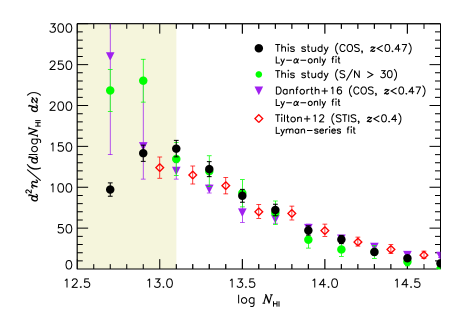
Figure 14: Comparisons between the four CDDF measurements per unit redshift $dz$ instead of $dX$ at the low-$N_{\mathrm{{\mathrm{H\,\mathsc{i}}}}}$ end. Incompleteness causes a turnover in our COS CDDF (filled circles) at $\log N_{\mathrm{{\mathrm{H\,\mathsc{i}}}}}$ $\sim$ 13.1 (the shaded region), while the incompleteness-corrected D16 COS CDDF continuously increases at $\log N_{\mathrm{{\mathrm{H\,\mathsc{i}}}}}$ $\leq$ 13.1. The CDDF calculated from the high-S/N subsample (green filled circles) used in Fig. 13 abruptly increases at $\log N_{\mathrm{{\mathrm{H\,\mathsc{i}}}}}$ $\sim$ 13.0. Note that the CDDF plotted depends both on $\log N_{\mathrm{{\mathrm{H\,\mathsc{i}}}}}$ and $\Delta N_{\mathrm{{\mathrm{H\,\mathsc{i}}}}}$.

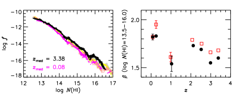
Figure 15: Left panel: The CDDF from the Lyman series fit at the seven redshift bins. The symbol sizes at $\tilde{z}$ $=$ 3.38 (highest $z$) and 0.08 (lowest $z$) are a factor of 2 larger to contrast the CDDF over the largest $z$ interval as its $z$-evolution is weak. The Poisson errors are not shown for clarity. Right panel: The CDDF slope $\beta$ measured at $\log N_{\mathrm{{\mathrm{H\,\mathsc{i}}}}}$ $\in$ [13.5, 16.0] from the Lyman series fit (filled circles) and the Ly-$\alpha$-only fit (open red squares). Only errors larger than the symbol size are plotted.

The left panel of Fig. 15 displays the redshift evolution of the overall shape of the CDDF. The CDDF shape at lower redshifts can be reproduced by a small amount of clockwise rotation of a higher-$z$ CDDF with a slightly larger CDDF normalisation $B$. This is caused by a fact that the number of H i absorbers decreases faster at higher $N_{\mathrm{{\mathrm{H\,\mathsc{i}}}}}$ and at lower $z$ with a self-similar manner in terms of the evolution of the large-scale structure and the degree of the IGM-galaxy interaction as a function of $z$.

The right panel indicates that the CDDF slope $\beta$ from the Lyman series fit in general becomes steeper as $z$ decreases, if the $\tilde{z}_{\alpha\beta}$ $=$ 1.03 CDDF is excluded due to the small-number statistics (Table 6). At $\tilde{z}_{\alpha\beta}$ $=$ 1.03, a very small $\Delta X$ coverage also decreases a probability of detecting less common H i absorbers at $\log N_{{\mathrm{H\,\mathsc{i}}}}$ $>$ 15.0. These lead to a factor of 3 larger statistical error than at other redshifts. This trend also holds for $\beta$ estimated from the Ly$\alpha$-only fit. On the other hand, the lower $\beta$ at $z\!\sim\!3$ compared to at the adjacent $z$ seems to be real as the number of analysed lines are large enough to obtain a reliable $\beta$. Due to a lack of data at $z\!>\!3.5$ we cannot discard a possibility of $\beta$ continuously increasing at $z\!=\!3\!\rightarrow\!4$ with a local minimum at $z\!\sim\!3$, which could be caused by a change in the IGM $N_{\mathrm{{\mathrm{H\,\mathsc{i}}}}}$ distribution due to extra heating and ionisation by He ii reionisation at $z\!\sim\!3$. (Reimers et al. 1997; Songaila 1998; Syphers & Shull 2013; Worseck et al. 2016).

5.2 The forest gas-phase mass density

One of the key cosmological parameters constrained by the IGM is the gas-phase hydrogen mass density relative to the critical density of the universe ($\Omega_{\mathrm{H}}$). This $\Omega_{\mathrm{H}}$ is model-dependent and is bound to be revised with an advent of more realistic models and with a better constraint on the UVB, the characteristic size of the IGM geometry and a density profile (Schaye 2001; Penton et al. 2004; Tilton et al. 2012). We used a simple method developed by Schaye (2001) to obtain a qualitative trend over time:

$$\Omega_{\mathrm{H}} \!\sim\! 2.2\!\times\!10^{-9}h^{-1}\Gamma_{12}^{1/3}\left({f_{g}\over 0.16}\right)^{1/3}\!T_{4}^{0.59}$$ (5)

$$\times\!\int\!N_{{\mathrm{H\,\mathsc{i}}}}^{1/3}f(N_{{\mathrm{H\,\mathsc{i}}}},dX)\,dN_{{\mathrm{H\,\mathsc{i}}}},$$

where $f_{g}$ is a mass fraction in gas-phase hydrogen, the hydrogen photoionisation rate $\Gamma_{12}\!\equiv\!\Gamma_{\mathrm{{\mathrm{H\,\mathsc{i}}}}}\!\times\!10^{-12}$ s^-1 and the gas temperature $T\!\equiv\!T_{4}\!\times\!10^{4}$ K, respectively, for our assumed cosmology $h=0.7$ (Schaye 2001). Strictly speaking, this holds only for overdense regions, i.e. $\log N_{{\mathrm{H\,\mathsc{i}}}}$ $\geq$ 13.5 at $z$ $\sim$ 3 and $\Omega_{\mathrm{H}}$ can be under-estimated by $\sim$20% at $\log N_{{\mathrm{H\,\mathsc{i}}}}$ $\leq$ 13.5 (Penton et al. 2004).

We directly integrated $f(N_{\mathrm{{\mathrm{H\,\mathsc{i}}}}},dX)$ as shown in Fig. 13 over several different column density ranges with the $\pm$1$\sigma$ Poisson errors. The model-independent factor 2.2 $\times$ $10^{-9}h^{-1}\!\int\!N_{HI}^{1/3}f(N_{HI},dX)\,dN_{HI}$ and the model-dependent $\Omega_{\mathrm{H}}$ are are tabulated in an online table on the MNRAS website (Table S3). The model-independent factor is a purely observational quantity and will not be likely to be changed significantly within our adopted column density range at $\log N_{{\mathrm{H\,\mathsc{i}}}}$ $\in$ [13, 16] in the near future. For the model-dependent $\Omega_{\mathrm{H}}$, $\Gamma_{12}$ is interpolated from the HM01 QG UVB at the given $z$, while $f_{g}$ and $T$ were interpolated from the IllustrisTNG simulation (Martizzi et al. 2019, their Table 1 and Fig. 4, respectively). For simplicity, we assume that the observed Ly$\alpha$ forest is mostly from the cool diffuse IGM and the halo gas in filaments and sheets and that the minimum temperature of simulated filaments at $\log n_{\mathrm{H}}\!=\!-4$ is a fair representative of the IGM temperature. An uncertainty of 10% in $\Gamma_{12}$, $f_{g}$ and $T_{4}$ changes $\Omega_{\mathrm{H}}$ by $\sim$3%, $\sim$3% and $\sim$6%, respectively, indicating that $T_{4}$ is the most important model-dependent parameter. However, the uncertainties associated with $T_{4}$ and $\Gamma_{12}$ are likely to be different, especially at low redshifts. Simulated distributions of H i line widths which are determined by gas temperature and non-thermal motion are not in agreement with observations by a factor of $\sim$2 at $z$ $\sim$ 0.1 (Viel et al. 2017). Several studies also suggest a factor of 2–5 larger $\Gamma_{12}$ than the widely-used theoretical prediction by Haardt & Madau (2012) at $z$ $\sim$ 0.2 (Kollmeier et al. 2014; Shull et al. 2015; Wakker et al. 2015; Khaire & Srianand 2019; Faucher-Giguère 2020).

Being fully consistent with previous studies, the low-$N_{\mathrm{{\mathrm{H\,\mathsc{i}}}}}$ absorbers at $\log N_{\mathrm{{\mathrm{H\,\mathsc{i}}}}}\!\in\![13,15]$ contain most baryons at $z$ $>$ 2.5, but their contribution decreases down to about 22% at $z$ $\sim$ 0 (Rauch et al. 1997; Shull et al. 2012; Danforth et al. 2016). The relative contribution to $\Omega_{\mathrm{b}}$ by absorbers at $\log N_{\mathrm{{\mathrm{H\,\mathsc{i}}}}}$ $\in$ [13.0, 14.5] and at $\log N_{\mathrm{{\mathrm{H\,\mathsc{i}}}}}$ $\in$ [14.5, 16.0] is about 4.5 at $z$ $\sim$ 0 and 2 at $z$ $\sim$ 3.4, which reflects a steeper slope of the CDDF at lower $z$. Due to incompleteness at $\log N_{\mathrm{{\mathrm{H\,\mathsc{i}}}}}$ $\sim$ 13, it is not currently possible to constrain the contribution to $\Omega_{\mathrm{b}}$ by these weaker absorbers.

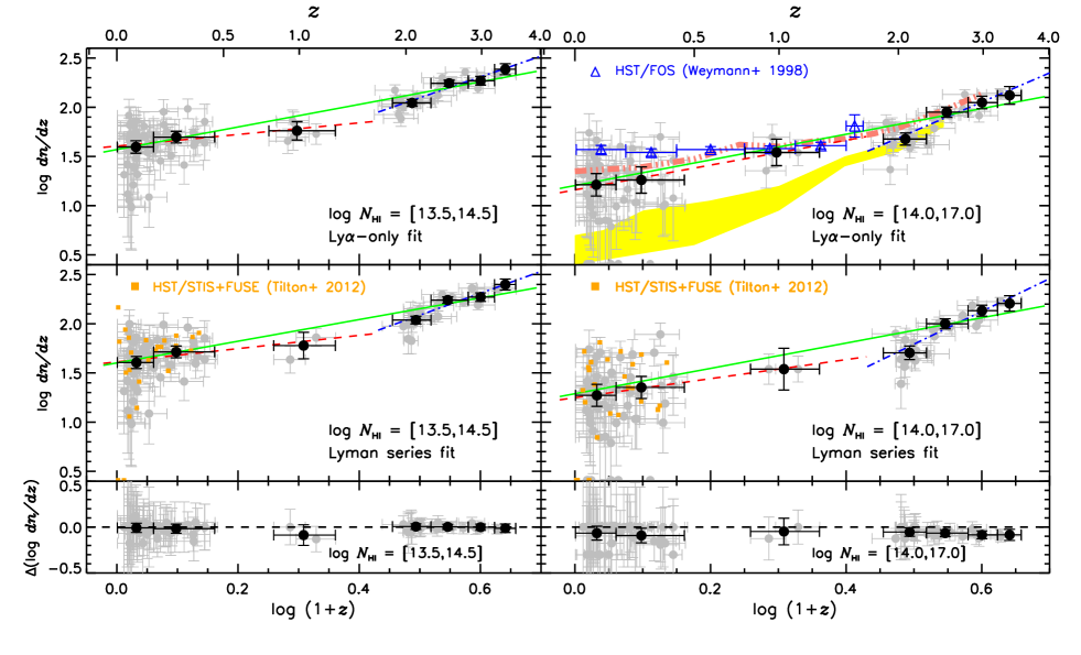
Figure 16: Left upper panel: The redshift evolution of the number of absorbers per unit $z$, $dn/dz$, from the Ly$\alpha$-only fit at $\log N_{\mathrm{{\mathrm{H\,\mathsc{i}}}}}$ $\in$ [13.5, 14.5]. The individual and averaged $dn/dz$ are shown as filled gray and black circles, respectively. The x-axis errors indicate the redshift range, while the y-axis errors are the 1$\sigma$ Poisson error accounting for lines with a questionable identification. The blue dot-dashed and red dashed lines are a best-fit single power law to the averaged $dn/dz$ at $z$ $>$ 1.5 and $z$ $<$ 1.5, respectively. The green solid line is a single power-law fit to the individual $dn/dz$ at 0 $<$ $z$ $<$ 3.6. Left middle panel: $dn/dz$ from the Lyman series fit. Left lower panel: The difference in $\log dn/dz$ between the Ly$\alpha$-only and Lyman series fits. The line number density $dn/dz$ from the Ly$\alpha$-only fit was recalculated over the same $z$ range used in the Lyman series fit. Right panels: Same as the left panels except for $\log N_{\mathrm{{\mathrm{H\,\mathsc{i}}}}}$ $\in$ [14, 17]. When there is no line, $\log dn/dz$ is set to be 0.41 without y-axis errors at the bottom of the panel. The open blue triangles are $dn/dz$ from HST/FOS spectra (Weymann et al. 1998), converted from equivalent width measurements assuming $b$ $=$ 25  km s^-1. In the upper panel, the yellow shade outlines the $dn/dz$ range from theoretical predictions by Davé et al. (2010) and Nasir et al. (2017), while the pink dot-dot-dot-dashed curve is a prediction by Davé et al. (1999).

5.3 Absorption line number density $dn/dz$

The H i absorber number density, $dn/dz$, is defined as the number of absorbers per unit redshift. It is proportional to the cross section and comoving number density of absorbers. It is usually measured over a specified H i column density range and its evolution as a function of $z$ is traditionally described as a single power law, $dn/dz$ $=$ $n_{0}\!\times\!(1\!+\!z)^{\gamma_{n}}$, where $n_{0}$ is the number density at $z$ $=$ 0.

Table 7: Averaged $dn/dz$

		$\log N_{\mathrm{{\mathrm{H\,\mathsc{i}}}}}\in[13.5,14.5]$			$\log N_{\mathrm{{\mathrm{H\,\mathsc{i}}}}}\in[14.0,17.0]$
$\log(1$ $+$ $\tilde{z})$	$dz$	# of			# of
		lines	$\log dn/dz$		lines	$\log dn/dz$
Ly$\alpha$-only fit
0.032${}_{-0.031}^{+0.029}$	3.926	155	1.60$\pm$0.03$\pm$0.03		64	1.21$\pm$0.05$\pm$0.06
0.098${}_{-0.037}^{+0.063}$	3.018	150	1.70$\pm$0.04$\pm$0.02		55	1.26$\pm$0.06$\pm$0.08
0.297${}_{-0.046}^{+0.063}$	1.267	73	1.76$\pm$0.05$\pm$0.04		44	1.54$\pm$0.07$\pm$0.07
0.487${}_{-0.032}^{+0.031}$	4.804	532	2.04$\pm$0.02$\pm$0.02		228	1.68$\pm$0.03$\pm$0.03
0.548${}_{-0.030}^{+0.031}$	3.281	575	2.24$\pm$0.02$\pm$0.01		292	1.95$\pm$0.03$\pm$0.03
0.600${}_{-0.021}^{+0.023}$	1.700	316	2.27$\pm$0.02$\pm$0.02		190	2.05$\pm$0.03$\pm$0.03
0.641${}_{-0.018}^{+0.017}$	0.703	171	2.39$\pm$0.03$\pm$0.02		93	2.12$\pm$0.05$\pm$0.05
Lyman series fit
0.032${}_{-0.032}^{+0.028}$	3.792	153	1.61$\pm$0.04$\pm$0.03		71	1.27$\pm$0.05$\pm$0.06
0.098${}_{-0.037}^{+0.063}$	3.018	156	1.71$\pm$0.04$\pm$0.03		70	1.37$\pm$0.05$\pm$0.06
0.308${}_{-0.049}^{+0.052}$	0.550	33	1.78$\pm$0.08$\pm$0.06		19	1.54$\pm$0.10$\pm$0.11
0.494${}_{-0.039}^{+0.025}$	3.709	404	2.04$\pm$0.02$\pm$0.02		188	1.70$\pm$0.03$\pm$0.04
0.546${}_{-0.028}^{+0.034}$	2.893	503	2.24$\pm$0.02$\pm$0.01		289	2.00$\pm$0.03$\pm$0.03
0.600${}_{-0.021}^{+0.023}$	1.700	317	2.27$\pm$0.02$\pm$0.02		231	2.13$\pm$0.03$\pm$0.03
0.641${}_{-0.018}^{+0.017}$	0.703	176	2.40$\pm$0.03$\pm$0.02		113	2.21$\pm$0.04$\pm$0.04

Due to the growth of structure, the same H i column density corresponds to a higher overdensity at lower $z$ (overdensity $\delta$ $=$ $\rho/\rho_{\mathrm{o}}$, where $\rho_{\mathrm{o}}$ is the cosmic mean matter density): $\log N_{\mathrm{{\mathrm{H\,\mathsc{i}}}}}$ $=$ 15 corresponds to $\delta$ $\sim$ 100 (inside halos) at $z$ $=$ 0 and $\delta$ $\sim$ 6 (the diffuse IGM) at $z$ $=$ 3 (Davé et al. 1999). In addition, star formation and feedback is predicted to affect the H i absorbers close to galaxies (Davé et al. 2010; Nasir et al. 2017). Therefore, $dn/dz$ is expected to change with $N_{\mathrm{{\mathrm{H\,\mathsc{i}}}}}$ and $z$, constraining structure evolution (Theuns et al. 1998a; Schaye 2001; Davé et al. 2010; Williger et al. 2010; Kim et al. 2013).

Figure 16 displays the $dn/dz$ evolution from the Ly$\alpha$-only (upper panels) and Lyman series (middle panels) fits at two different $N_{\mathrm{{\mathrm{H\,\mathsc{i}}}}}$ ranges, at $\log N_{\mathrm{{\mathrm{H\,\mathsc{i}}}}}$ $\in$ [13.5, 14.5] (left panels) and at $\log N_{\mathrm{{\mathrm{H\,\mathsc{i}}}}}$ $\in$ [14, 17] (right panels), respectively. The criterion of $S/N\!>\!18$ for COS/STIS spectra enables detection of H i at $\log N_{\mathrm{{\mathrm{H\,\mathsc{i}}}}}$ $\leq$ 13. However, since the $N_{\mathrm{{\mathrm{H\,\mathsc{i}}}}}$ detection limit varies with $b$ and the two sightlines at $z$ $\sim$ 1 have $S/N$ $\sim$ 10–18, to be conservative we use a lower $N_{\mathrm{{\mathrm{H\,\mathsc{i}}}}}$ limit of $\log N_{\mathrm{{\mathrm{H\,\mathsc{i}}}}}$ $=$ 13.5.

The most striking feature of $dn/dz$ in the upper and middle panels of Fig. 16 is a large scatter in individual $dn/dz$ (gray filled circles, tabulated in the supplementary online Tables S4 and S5 on the MNRAS webpage) at any given redshift for both $N_{\mathrm{{\mathrm{H\,\mathsc{i}}}}}$ ranges. The scatter becomes larger at lower redshifts, spanning about an order of magnitude at $z$ $\sim$ 0 (Fig. 17). About half the COS AGN sightlines at $z$ $<$ 0.5 do not contain an absorber at $\log N_{\mathrm{{\mathrm{H\,\mathsc{i}}}}}$ $\geq$ 14.5. At the same time, Fig. 17 indicates that 9% (5/55) of sightlines at $z$ $<$ 0.5 contain more absorbers with $\geq$8$\sigma$ at $\log N_{\mathrm{{\mathrm{H\,\mathsc{i}}}}}$ $\in$ [13.5, 14.5] than the averaged $dn/dz$, compared to none at $z$ $>$ 1.5. The contrast between extremely high and low $dn/dz$ becomes more prominent at a higher column density range and at low redshifts. A $dn/dz$ study based on 27 STIS/FUSE spectra at $z$ $>$ 0.02 (Tilton et al. 2012, filled orange squares) is consistent with our individual COS $dn/dz$: although the STIS resolution is 3 times higher, its S/N is much lower and a different method was used for estimating $N_{\mathrm{{\mathrm{H\,\mathsc{i}}}}}$. Even though not shown, the D16 individual $dn/dz$ also shows a large scatter.

This large scatter is in part intrinsic caused by a stronger clustering of stronger absorbers (a large positive $\sigma_{dn/dz}$ combined with a sightline without strong absorbers) toward lower $z$ as a result of structure evolution, cooled-down galactic outflows near star-forming galaxies and enhanced H i ionizing photons (Dobrzycki et al. 2002; Dall’Aglio et al. 2008; Davé et al. 2010; Nasir et al. 2017). The scatter is also in part caused by the different $z$ coverage for each sightline. This redshift coverage bias is especially significant at $z$ $\sim$ 0 and $z$ $\sim$ 2 as the wavelength coverage is smaller due to the rest-frame Ly$\alpha$ and atmospheric cutoffs, respectively. The large scatter due to both cosmic variance and redshift coverage bias implies that the $dn/dz$ study requires many sightlines, especially at lower $z$. A small sample size is the primary reason of the earlier discrepancy between the FOS and STIS $dn/dz$ studies as the STIS $dn/dz$ was measured using only a few sightlines (Lehner et al. 2007; Williger et al. 2010).

Figure 17: Deviation of the individual $dn/dz$ from the averaged $dn/dz$ for the Lyman series fit. The deviation is calculated using the Poisson error of the averaged $dn/dz$ within a given redshift range $\Delta z$ excluding the sightline in consideration: $\Delta z$ $=$ 0.05 at $z$ $<$ 0.45, $\Delta z$ $=$ 0.48 at $z$ $\sim$ 1, $\Delta z$ $=$ 0.2 at 1.9 $<$ $z$ $<$ 3.0 and $\Delta z$ $=$ 0.35 at 3.0 $<$ $z$ $<$ 3.6, respectively. For a sightline without H i absorbers in a given column density range, $\sigma_{dn/dz}$ is assigned to be $-10$ with gray circles. The positive deviation indicates that the sightline contains more H i absorbers than the averaged $dn/dz$.

While the parameter space occupied by individual $dn/dz$ measurements on the $z$–$dn/dz$ plane is important for constraining the inhomogeneity of H i distribution, the averaged $dn/dz$ (filled circles) is a better quantity to directly compare to simulations which usually average thousands of sightlines. To reduce redshift coverage bias, the averaged $dn/dz$ is measured from the combined line lists of all the AGN per $N_{\mathrm{{\mathrm{H\,\mathsc{i}}}}}$ and per $z$ instead of an arithmetic mean. Considering the large scatter in the individual $dn/dz$, the commonly-used Poisson errors seem to underestimate the real errors. Therefore, we include the bootstrap error measured from the combined lines for each $z$ bin in addition to the Poisson errors. The averaged $dn/dz$ is tabulated in Table 7 with the first $dndz$ error being the Poisson error and the second error being 0.5 times the standard deviation.

In Fig. 16, the green solid line is a single power-law fit to the individual $dn/dz$ at $0$ $<$ $z$ $<$ 3.6. Due to the large scatter at a given $z$, this single power-law fit roughly describes the overall individual $dn/dz$ evolution, although a underprediction of $dn/dz$ is suggested at $z$ $>$ 3.6. The blue dot-dashed line shows a best-fit single power law to the averaged $dn/dz$ at $z$ $>$ 1.5. At both $N_{\mathrm{{\mathrm{H\,\mathsc{i}}}}}$ ranges for the Ly$\alpha$-only and Lyman series fits, this fit underpredicts the $dn/dz$ at $z$ $<$ 0.5 (Weymann et al. 1998; Kim et al. 2013). The discrepancy is larger at the higher-$N_{\mathrm{{\mathrm{H\,\mathsc{i}}}}}$ range, since stronger absorbers are expected to disappear more rapidly at lower $z$ when extrapolated from high $z$. The red dashed lines represents a best-fit single power law to the averaged $dn/dz$ at $z$ $<$ 1.5. This fit underpredicts the observed $dn/dz$ at $z$ $>$ 1.5. The fit parameters are listed in Table 8. Note that there is no significant difference between the single power-law fits to the averaged $dn/dz$ (not shown) and the individual $dn/dz$ (green solid line).

For both $N_{\mathrm{{\mathrm{H\,\mathsc{i}}}}}$ ranges, the inadequacy of a single power-law fit is consistent with the evolution of $<$$F$$>$ and the PDF – there exists an IGM evolutionary break at $z$ $\sim$ 1.5–1.7 and the stronger absorbers evolve more strongly, i.e. a larger $\gamma_{n}$ (Theuns et al. 1998a; Scott et al. 2000; Kim et al. 2013). Ribaudo et al. (2011) find that the averaged $dn/dz$ of Lyman limit systems at $\log N_{\mathrm{{\mathrm{H\,\mathsc{i}}}}}$ $\geq$ 17.5 at $0.0$ $<$ $z$ $<$ 2.6 is well described with $\gamma_{n}$ $=$ 1.33$\pm$0.61. Although the errors are large for both studies and their $dn/dz$ does not show any evolutionary break at $z$ $\sim$ 1.5, their $\gamma_{n}$ combined with ours at 0 $<$ $z$ $<$ 3.6 at $\log N_{\mathrm{{\mathrm{H\,\mathsc{i}}}}}$ $\in$ [13.5, 14.0] ($\gamma_{n}$ $\sim$ 1.10) and [14.0, 17.0] ($\gamma_{n}$ $\sim$ 1.27) suggests that $\gamma_{n}$ increases with $N_{\mathrm{{\mathrm{H\,\mathsc{i}}}}}$.

At $\log N_{\mathrm{{\mathrm{H\,\mathsc{i}}}}}$ $\in$ [14, 17] (right upper panel), the yellow shade represents the predicted $dn/dz$ evolution in terms of $N_{\mathrm{{\mathrm{H\,\mathsc{i}}}}}$ instead of the equivalent width, compiled from various simulations from outflow models to no-wind models under a quasars+galaxies UVB (Davé et al. 2010; Nasir et al. 2017). As outflows eject the processed gas into halos, which subsequently cools down and produces strong absorbers, outflow models tend to predict higher $dn/dz$. However, it is clear that these models significantly underpredict the observed $dn/dz$ by a factor of $\sim$3–5, suggesting that saturated Ly$\alpha$ absorbers at low redshift are not yet correctly simulated.

In the same panel, the pink dot-dot-dot-dashed line is a predicted $dn/dz$ by Davé et al. (1999) under the quasars-only UVB. Their prediction is in a strikingly good agreement with our measurement. This can indicate that the quasars-only UVB is more preferable than the quasars+galaxies UVB under which latest simulations including more recent models by Davé et al. (2010) do not reproduce the observations. However, this comparison is potentially complicated by the fact that their $\Lambda$-CDM model is based on outdated cosmological parameters such as $\Omega_{\Lambda}$ $=$ 0.6 without incorporating any extra heating source such as He ii photo-heating at $z$ $>$ 2 (Syphers & Shull 2013; Worseck et al. 2016; Nasir et al. 2017) nor any stellar/AGN feedback. The simulation includes only $64^{3}$ particles in a small box of side length 11$h^{-1}$ comoving Mpc so that it does not resolve the IGM gas particles as well as some of current IGM simulations (Davé et al. 2010; Nasir et al. 2017; Martizzi et al. 2019).

The lower left panel displays the difference in $dn/dz$ between the Ly$\alpha$-only and Lyman series fits. At $\log N_{\mathrm{{\mathrm{H\,\mathsc{i}}}}}$ $\in$ [13.5, 14.5], a few individual sightlines display a difference up to $\sim$20%. However, there is no noticeable difference in the average except at $z$ $\sim$ 1 where the averaged $dn/dz$ suffers from small number statistics. At $\log N_{\mathrm{{\mathrm{H\,\mathsc{i}}}}}$ $\geq$ 14.5, Ly$\alpha$ lines start to saturate in the UVES/HIRES spectra. Since some saturated lines can be resolved into several weaker components in higher order lines and since the Ly$\alpha$-only fit in general gives a lower $N_{\mathrm{{\mathrm{H\,\mathsc{i}}}}}$ limit for saturated lines, the difference between the two sets becomes more noticeable at higher $N_{\mathrm{{\mathrm{H\,\mathsc{i}}}}}$ (lower right panel). At $\log N_{\mathrm{{\mathrm{H\,\mathsc{i}}}}}$ $\in$ [14, 17], the $dn/dz$ from the Lyman series fit is about a factor of 1.2 larger than from the Ly$\alpha$-only fit.

Table 8: Power-law fit parameters to the number density $dn/dz$

	Ly$\alpha$-only fit		Lyman series fit
$\log N_{\mathrm{{\mathrm{H\,\mathsc{i}}}}}$	$\log n_{\mathrm{0}}$	$\gamma_{n}$	$\log n_{\mathrm{0}}$	$\gamma_{n}$
	0 $<$ $z$ $<$ 3.6 for the individual $dn/dz$
13.5–14.5	1.57$\pm$0.03	1.15$\pm$0.05	1.60$\pm$0.03	1.10$\pm$0.05
14.0–17.0	1.20$\pm$0.04	1.30$\pm$0.08	1.29$\pm$0.04	1.28$\pm$0.07
	$z$ $>$ 1.5 for the averaged $dn/dz$
13.5–14.5	1.04$\pm$0.20	2.12$\pm$0.37	0.97$\pm$0.23	2.23$\pm$0.41
14.0–17.0	0.27$\pm$0.34	2.96$\pm$0.61	0.13$\pm$0.36	3.33$\pm$0.64
	$z$ $<$ 1.5 for the averaged $dn/dz$
13.5–14.5	1.61$\pm$0.06	0.59$\pm$0.42	1.61$\pm$0.06	0.67$\pm$0.53
14.0–17.0	1.16$\pm$0.11	1.26$\pm$0.65	1.25$\pm$0.11	0.97$\pm$0.87

6 Conclusions

We performed a new uniform, consistent Voigt profile fitting analysis on the 84 high-quality AGN spectra from the HST/COS, HST/STIS, VLT/UVES and Keck/HIRES archives in order to characterise the redshift evolution of the transmitted flux $F$ and column density of neutral hydrogen H i of the low-density IGM at 0 $<$ $z$ $<$ 3.6. Although this data set does not sample the IGM continuously in redshift space, the selected redshift ranges are the best compromise within the capabilities of currently available ground-based and space-based spectrographs:

• VLT-UVES/Keck I-HIRES set consists of 24 QSO spectra with a resolution of $\sim$6.7  km s^-1 and a S/N ratio per resolution element of 40–250, sampling the IGM at 1.7 $<$ $z$ $<$ 3.6 with the total $z$ coverage $\Delta z$ $=$ 11.59 for the Ly$\alpha$-only fit range. The typical $N_{\mathrm{{\mathrm{H\,\mathsc{i}}}}}$ detection limit is $\log N_{\mathrm{{\mathrm{H\,\mathsc{i}}}}}$ $\sim$ 12.5.

• HST/STIS+COS NUV set covers the IGM at $z$ $\sim$ 1 with $\Delta z$ $=$ 1.27 (the Ly$\alpha$-only fit). The set includes two QSO spectra from the HST/STIS archive supplemented with our new observations of three QSO spectra taken with the HST/COS NUV G225M grating. The approximated Gaussian resolution of STIS E230M and COS NUV spectra is $\sim$10  km s^-1 and $\sim$12  km s^-1, respectively, with a non-Gaussian wing. The $S/N$ range is $\sim$13–46. The $\log N_{\mathrm{{\mathrm{H\,\mathsc{i}}}}}$ detection limit is $\sim$13.

• HST/COS FUV set has 55 AGN spectra with $S/N$ $\sim$ 18–85 covering the IGM at 0 $<$ $z$ $<$ 0.5 with $\Delta z$ $=$ 7.20 (the Ly$\alpha$-only fit). The resolution can be approximated to $\sim$19  km s^-1 with a non-Gaussian wing. The $\log N_{\mathrm{{\mathrm{H\,\mathsc{i}}}}}$ detection limit is $\sim$13.

For the continuous flux statistics, we used artificial spectra generated from the Ly$\alpha$-only fit since it can use a larger wavelength range than the Lyman series fit for which the useful wavelength is sometimes shortened due to the need for coverage of high-order Lyman lines. The generated spectra also enable to combine the COS/STIS spectra having a non-Gaussian line spread function with the UVES/HIRES data having a Gaussian one and to remove the metal contamination. Our consistent analysis based on the best data currently available confirms previous findings qualitatively (Weymann et al. 1998; Penton et al. 2004; Lehner et al. 2007; Tilton et al. 2012; Danforth et al. 2016) and provides more robust quantitative results. We have found:

1. The mean transmitted H i flux is not sensitive to S/N, nor supposedly undetected weak lines due to noise. While the flux PDF (probability distribution function, the fraction of pixels having a given normalized flux $F$) is not sensitive to undetected weak lines, the flux PDF is directly comparable among different S/N data only at 0.1 $<$ $F$ $<$ 0.7.

2. The mean H i flux increases fast at $z$ $=$ 3.6 $\rightarrow$ 1.5, slows down at $z$ $\sim$ 1, then does not show any significant change at $z$ $=$ 0.5 $\rightarrow$ 0.0. A best-fit double power-law to the individual $<$$F$$>$ measurements is $\ln<$$F$$>$ $=$ $(-0.0145\pm 0.0003)\times(1+z)^{1.86\pm 0.07}$ at $z$ $<$ 1.5 and $\ln<$$F$$>$ $=$ $(-0.0040\pm 0.0001)\times(1+z)^{3.18\pm 0.02}$ at $z$ $>$ 1.5, respectively.

3. The mean PDF as a function of $F$ and $z$, $<$$P(F,z)$$>$, qualitatively suggests that the volume fraction occupied by flux voids ($F$ $\sim$ 1) increases rapidly at $z$ $=$ 3.6 $\rightarrow$ 1.5, then increases slowly at $z$ $<$ 1.5. With no absorption defined as $F$ $=$ 1, this evolution reflects the thinning of the forest toward lower redshift, due to the evolution in the gas proper density and the intensity of the UV background.

For the $N_{\mathrm{{\mathrm{H\,\mathsc{i}}}}}$ distribution, we used the Lyman series fit for more reliable determination of $N_{\mathrm{{\mathrm{H\,\mathsc{i}}}}}$ for saturated H i Ly$\alpha$. For the UV spectra taken with the HST, a corresponding non-Gaussian LSF provided for each instrument setting and observation date is used. At $\log N_{\mathrm{{\mathrm{H\,\mathsc{i}}}}}$ $\in$ [13.5, 16.0] where incompleteness is negligible, 24 UVES/HIRES spectra at 1.9 $<$ $z$ $<$ 3.6, two STIS+three COS NUV spectra at $z$ $\sim$ 1 and 55 COS FUV spectra at 0 $<$ $z$ $<$ 0.45 provide 1798 (2043), 39 (93) and 371 (360) H i lines, respectively, for the Lyman series (Ly$\alpha$-only) fit. We have found:

1. The redshift evolution of the column density distribution function (CDDF), albeit weak over a small $z$ range, is such that the overall shape of the CDDF at lower redshifts can be reproduced by a small amount of clockwise rotation of a higher-$z$ CDDF with a slightly larger normalisation (bottom panels of Fig. 13 and left panel of Fig. 15).

2. For a conventional fit to the CDDF, $f$ $\propto$ $N_{\mathrm{{\mathrm{H\,\mathsc{i}}}}}^{-\beta}$, the slope $\beta$ at $\log N_{\mathrm{{\mathrm{H\,\mathsc{i}}}}}$ $\in$ [13.5, 16.0] in general becomes steeper at lower $z$: $\beta$ $=$ 1.60$\pm$0.02 at $z$ $\sim$ 3.4 and $\beta$ $=$ 1.82$\pm$0.03 at $z$ $\sim$ 0.1. This reflects that higher-$N_{\mathrm{{\mathrm{H\,\mathsc{i}}}}}$ absorbers disappear more rapidly and decrease in number or cross-section over time.

3. The slope $\beta$ is lower than the overall trend at $z$ $\sim$ 1 where an evolutionary break in the flux statistics is seen and at $z$ $\sim$ 3. The deviation at $z$ $\sim$ 1 could be spurious due to the small sample size, while the deviation at $z$ $\sim$ 3 could be caused by a change in the $N_{\mathrm{{\mathrm{H\,\mathsc{i}}}}}$ distribution due to extra heating and ionisation by the hypothetical He ii reionisation at $z$ $\sim$ 3. A further study with more data at $z$ $\sim$ 1 and at $z$ $>$ 3.6 is required to confirm the $\beta$ deviation.

4. The individual $dn/dz$ (the number of absorbers per unit $z$) shows a large scatter at a given $z$. The scatter increases toward lower $z$ and spans about an order of magnitude at $z$ $\sim$ 0, possibly caused by a combination of a stronger clustering at lower $z$, outflows near star-forming galaxies, locally enhanced H i ionization rates and a shorter redshift coverage of some sightlines.

5. The averaged $dn/dz$ ($dn/dz$ $\propto$ $(1\!+\!z)^{\gamma_{n}}$) is described better with a double power-law fit with an evolutionary break at $z$ $\sim$ 1.5, consistent with the evolution of transmitted flux. For the more reliable Lyman series fit, at $N_{\mathrm{{\mathrm{H\,\mathsc{i}}}}}$ $\in$ [13.5, 14.5], $\gamma_{n}$ $=$ 2.23$\pm$0.41 at $z$ $>$ 1.5 and $\gamma_{n}$ $=$ 0.67$\pm$0.53 at $z$ $<$ 1.5, while at $N_{\mathrm{{\mathrm{H\,\mathsc{i}}}}}$ $\in$ [14, 17], $\gamma_{n}$ $=$ 3.33$\pm$0.64 at $z$ $>$ 1.5 and $\gamma_{n}$ $=$ 0.97$\pm$0.87 at $z$ $<$ 1.5, consistent with the rapid disappearance of higher-$N_{\mathrm{{\mathrm{H\,\mathsc{i}}}}}$ absorbers with time.

7 Data availability

The data underlying this article are available in the article and in its online supplementary material. When the fitted line parameters will be completely analysed in our future papers, the entire fitted line list will be available online.

References

- Altay et al. (2011) Altay G., Theuns T., Schaye J., Crighton N. H. M., Dalla Vecchia C., 2011, ApJ, 737, L37
- Bahcall & Peebles (1969) Bahcall J. N., Peebles P. J. E., 1969, ApJ, 156, L7
- Becker et al. (2013) Becker G. D., Hewett P. C., Worseck G., Prochaska J. X., 2013, MNRAS, 430, 2067
- Boksenberg & Sargent (2015) Boksenberg A., Sargent W. L. W., 2015, ApJS, 218, 7
- Bolton et al. (2005) Bolton J. S., Haehnelt M. G., Viel M., Springel V., 2005, MNRAS, 357, 1178
- Bolton et al. (2008) Bolton J. S., Viel M., Kim T.-S., Haehnelt M. G., Carswell R. F., 2008, MNRAS, 386, 1131
- Calura et al. (2012) Calura F., Tescari E., D’Odorico V., Viel M., Cristiani S., Kim T.-S., Bolton J. S., 2012, MNRAS, 422, 3019
- Carswell & Webb (2014) Carswell R. F., Webb J. K., 2014, VPFIT, Astrophysics Source Code Library, record ascl:1408.015,
- Carswell et al. (1987) Carswell R. F., Webb J. K., Baldwin J. A., Atwood B., 1987, ApJ, 319, 709
- Carswell et al. (2002) Carswell R. F., Schaye J., Kim T. S., 2002, ApJ, 578, 43
- Cen & Ostriker (1999) Cen R., Ostriker J. P., 1999, ApJ, 514, 1
- Cen et al. (1994) Cen R., Miralda-Escudé J., Ostriker J. P., Rauch M., 1994, ApJl, 437, L9
- Dall’Aglio et al. (2008) Dall’Aglio A., Wisotzki L., Worseck G., 2008, A&A, 480, 359
- Danforth et al. (2010) Danforth C. W., Stocke J. T., Shull J. M., 2010, ApJ, 710, 613
- Danforth et al. (2016) Danforth C. W., Keeney B. A., Tilton E. M., Shull J. M., Stocke J. T., Stevans M., Pieri M. M., Savage B. D. e. a., 2016, ApJ, 817, 111
- Dashtamirova et al. (2019) Dashtamirova et al. 2019, Cosmic Origins Spectrograph Instrument Handbook, Version 12.0 (Baltimore: STScI)
- Davé et al. (1999) Davé R., Hernquist L., Katz N., Weinberg D. H., 1999, ApJ, 511, 521
- Davé et al. (2010) Davé R., Oppenheimer B. D., Katz N., Kollmeier J. A., Weinberg D. H., 2010, MNRAS, 408, 2051
- Dekker et al. (2000) Dekker H., D’Odorico S., Kaufer A., Delabre B., Kotzlowski H., 2000, SPIE, 4008, 534
- Dobrzycki et al. (2002) Dobrzycki A., Bechtold J., Scott J., Morita M., 2002, ApJ, 571, 654
- Ebbets (1995) Ebbets D., 1995, in Koratkar A., Leitherer C., eds, Proc. STScI Workshop, Calibrating Hubble Space Telescope: Post Servicing Mission, Space Telescope Science Institute, Baltimore, p. 207
- Faucher-Giguère (2020) Faucher-Giguère C., 2020, MNRAS, 493, 1614
- Faucher-Giguére et al. (2008a) Faucher-Giguére C.-A., Prochaska J. X., Lidz A., Hernquist L., Zaldarriaga M., 2008a, ApJ, 681, 831
- Faucher-Giguère et al. (2008b) Faucher-Giguère C., Lidz A., Hernquist L., Zaldarriaga M., 2008b, ApJ, 688, 85
- Fitzpatrick & Spitzer (1994) Fitzpatrick E. L., Spitzer L. J., 1994, ApJ, 427, 232
- Ford et al. (2013) Ford A. B., Oppenheimer B. D., Davé R., Katz N., Kollmeier J. A., Weinberg D. H., 2013, MNRAS, 432, 89
- Fukugita et al. (1998) Fukugita M., Hogan C. J., Peebles P. J. E., 1998, ApJ, 503, 518
- Gaikwad et al. (2019) Gaikwad P., Srianand R., Khaire V., Choudhury T. R., 2019, MNRAS, 490, 1588
- Gurvich et al. (2017) Gurvich A., Burkhart B., Bird S., 2017, ApJ, 835, 175
- Haardt & Madau (2012) Haardt F., Madau P., 2012, ApJ, 746, 125
- Haider et al. (2016) Haider M., Steinhauser D., Vogelsberger M., Genel S., Springel V., Torrey P., Hernquist L., 2016, MNRAS, 457, 3024
- Hiss et al. (2018) Hiss H., Walther M., Hennawi J. F., Oñorbe J., O’Meara J. M., Rorai A., Lukić J., 2018, ApJ, 865, 42
- Hu et al. (1995) Hu E. M., Kim T., Cowie L. L., Songaila A., Rauch M., 1995, AJ, 110, 1526
- Hui & Gnedin (1997) Hui L., Gnedin N. Y., 1997, MNRAS, 292, 27
- Janknecht et al. (2006) Janknecht E., Reimers D., Lopez S., Tytler D., 2006, A&A, 458, 427
- Jarosik et al. (2011) Jarosik N., et al., 2011, ApJS, 192
- Jenkins & Ostriker (1991) Jenkins E. B., Ostriker J. P., 1991, ApJ, 376, 33
- Keeney et al. (2012) Keeney B. A., Danforth C. W., Stocke J. T., France K., Green J. C., 2012, pasp, 124, 830
- Khaire & Srianand (2019) Khaire V., Srianand R., 2019, MNRAS, 484, 4174
- Kim et al. (1997) Kim T., Hu E. M., Cowie L. L., Songaila A., 1997, AJ, 114, 1
- Kim et al. (2007) Kim T., Bolton J. S., Viel M., Haehnelt M. G., Carswell R. F., 2007, MNRAS, 382, 1657
- Kim et al. (2013) Kim T.-S., Partl A. J., Carswell R. F., Müller V., 2013, å, 731, 6
- Kim et al. (2016) Kim T.-S., Carswell R. F., Mongardi C., Partl A., Mücket J. P., Barai P., Cristiani S., 2016, MNRAS, 770, 138
- Kirkman & Tytler (1997) Kirkman D., Tytler D., 1997, ApJ, 484, 672
- Kirkman et al. (2007) Kirkman D., Tytler D., Lubin D., Charlton J., 2007, MNRAS, 376, 1227
- Kollmeier et al. (2014) Kollmeier J. A., Weinberg D. H., Oppenheimer B. D., Haardt F., Katz N., Dav’e R., Fardal M. e. a., 2014, ApJ, 789, 32
- Kriss (2011) Kriss G. A., 2011, COS Instrument Science Report 2011-01
- Lee (2012) Lee K.-G., 2012, ApJ, 753, 136
- Lehner et al. (2007) Lehner N., Savage B. D., Richter P., Sembach K. R., Tripp T. M., Wakker B. P., 2007, ApJ, 658, 680
- Lidz et al. (2006) Lidz A., Heitmann K., Hui L., Habib S., Rauch M., Sargent W. L. W., 2006, ApJ, 638, 27
- Martizzi et al. (2019) Martizzi D., et al., 2019, MNRAS, 486, 3766
- McDonald et al. (2000) McDonald P., Miralda-Escudé J., Rauch M., Sargent W. L. W., Barlow T. A., Cen R., Ostriker J. P., 2000, ApJ, 543, 1
- McDonald et al. (2001) McDonald P., Miralda-Escudé J., Rauch M., Sargent W. L. W., Barlow T. A., Cen R., 2001, ApJ, 562, 52
- Nasir et al. (2017) Nasir F., Bolton J. S., Viel M., Kim T.-S., Haehnelt M. G., Puchwein E., Sijacki D., 2017, MNRAS, 471, 1056
- Noterdaeme et al. (2009) Noterdaeme P., Petitjean P., Ledoux C., Srianand R., 2009, A&A, 505, 1087
- Oñorbe et al. (2017) Oñorbe J., Hennawi J. F., Lukić J., 2017, ApJ, 837, 106
- O’Meara et al. (2013) O’Meara J. M., Prochaska J. X., Worseck G., Chen H.-W., Madau P., 2013, ApJ, 765, 137
- Paschos et al. (2009) Paschos P., Jena T., Tytler D., Kirkman D., Norman M. L., 2009, MNRAS, 399, 1934
- Peeples et al. (2010) Peeples M. S., Weinberg D. H., Davé R., 2010, MNRAS, 404, 1281
- Penton et al. (2000) Penton S. V., Shull J. M., Stocke J. T., 2000, ApJ, 544, 150
- Penton et al. (2004) Penton S. V., Stocke J. T., Shull J. M., 2004, ApJS, 152, 29
- Petitjean et al. (1993) Petitjean P., Webb J. K., Rauch M., Carswell R. F., Lanzetta K., 1993, MNRAS, 262, 499
- Planck collaboration (2016) Planck collaboration e. a., 2016, A&A, 594
- Prochaska et al. (2010) Prochaska J. X., OḾeara J. M., Worseck G., 2010, ApJ, 718, 392
- Puchwein et al. (2019) Puchwein E., Haardt F., Haehnelt M. G., Madau P., 2019, MNRAS, 485, 47
- Rahmati et al. (2012) Rahmati A., Pawlik A. H., Raičevic̀ O., Schaye J., 2012, MNRAS, 423, 149
- Rauch et al. (1997) Rauch M., et al., 1997, ApJ, 489, 7
- Reimers et al. (1997) Reimers D., Kohler S., Wisotzki L., Groote D., Rodriguez-Pascual P., Wamsteker W., 1997, aa, 327, 890
- Ribaudo et al. (2011) Ribaudo J., Lehner L., Howk J. C., 2011, ApJ, 736, 42
- Riley (2018) Riley A. e. a., 2018, “STIS Instrument Handbook”, Version 17.0, (Baltimore:STScI)
- Rollinde et al. (2013) Rollinde E., Theuns T., Schaye J., Pâris I., Petitjean P., 2013, MNRAS, 428, 540
- Rudie et al. (2013) Rudie G. C., Steidel C. C., Shapley A. E., Pettini M., 2013, ApJ, 769, 146
- Sargent et al. (1980) Sargent W. L. W., Young P. J., Boksenberg A., Tytler D., 1980, ApJS, 42, 41
- Savage & Sembach (1991) Savage B. D., Sembach K. R., 1991, ApJ, 379, 245
- Savage et al. (2014) Savage B. D., Kim T. S., Wakker B. P., Keeney B., Shull J. M., Stocke J. T., Green J. C., 2014, ApJS, 212, 8
- Savaglio et al. (1999) Savaglio S., et al., 1999, ApJl, 515, L5
- Schaye (2001) Schaye J., 2001, ApJ, 559, 507
- Scott et al. (2000) Scott J., Bechtold J., Dobrzycki A., 2000, ApJS, 130, 37
- Sembach & Savage (1992) Sembach K. R., Savage B. D., 1992, ApJS, 83, 147
- Sembach et al. (1991) Sembach K. R., Savage B. D., Massa D., 1991, ApJ, 372, 81
- Shen et al. (2012) Shen S., Madau P., Aguirre A., Guedes J., Mayer L., Wadsley J., 2012, ApJ, 760, 50
- Shull et al. (2000) Shull J. M., et al., 2000, ApJL, 538, 13
- Shull et al. (2012) Shull M., Smith B. D., Danforth C. W., 2012, ApJ, 759, 23
- Shull et al. (2015) Shull J. M., Maloney J., Danforth C. W., Tilton E. M., 2015, ApJ, 811, 3
- Songaila (1998) Songaila A., 1998, AJ, 115, 2184
- Steidel et al. (2010) Steidel C. C., Erb D. K., Shapley A. E., Pettini M., Reddy N., Bogosavljević M., Rudie G. C., Rakic O., 2010, ApJ, 717, 289
- Suresh et al. (2015) Suresh J., Bird S., Vogelsberger M., Genel S., Torrey P., Sijacki D., Springel V., Hernquist L., 2015, MNRAS, 448, 895
- Syphers & Shull (2013) Syphers D., Shull J. M., 2013, ApJ, 765, 119
- Tepper-García et al. (2012) Tepper-García T., Richter P., Schaye J., Booth C. M., Dalla Vecchia C., Theuns T., 2012, MNRAS, 425, 1640
- Theuns et al. (1998a) Theuns T., Leonard A., Efstathiou G., 1998a, MNRAS, 297, L49
- Theuns et al. (1998b) Theuns T., Leonard A., Efstathiou G., Pearce F. R., Thomas P. A., 1998b, MNRAS, 301, 478
- Tilton et al. (2012) Tilton E. M., Danforth C. W., Shull J. M., Ross T. L., 2012, ApJ, 759, 112
- Tripp et al. (2008) Tripp T. M., Sembach K. B., Bowen D. V., Savage B. D., Jenkins E. B., Lehner N., Richter P., 2008, ApJS, 177, 39
- Viel et al. (2017) Viel M., Haehnelt M. G., Bolton J. S., Kim T.-S., Puchwein E., Nasir F., Wakker B. P., 2017, MNRAS, 467, 86
- Vogt (1994) Vogt S. S. e. a., 1994, Proc. SPIE, 2198, 362
- Vogt (2002) Vogt S. S., 2002, ASPC, 270, 5
- Wakker (2006) Wakker B. P., 2006, ApJS, 163, 282
- Wakker & Savage (2009) Wakker B. P., Savage B. D., 2009, ApJS, 182, 378
- Wakker et al. (2015) Wakker B. P., Hernandez A. K., French D. M., Kim T.-S., Oppenheimer B. D., Savage B. D., 2015, ApJ, 814, 40
- Weymann et al. (1998) Weymann R. J., et al., 1998, ApJ, 506, 1
- Williger et al. (2010) Williger G. M., et al., 2010, MNRAS, 405, 1736
- Worseck et al. (2016) Worseck G., Prochaska J. X., Hennawi J. F., McQuinn M., 2016, ApJ, 825, 144