Charging power and stability of always-on transitionless driven quantum batteries

Abstract

The storage and transfer of energy through quantum batteries are key elements in quantum networks. Here, we propose a charger design based on transitionless quantum driving (TQD), which allows for inherent control over the battery charging time, with the speed of charging coming at the cost of the internal energy available to implement the dynamics. Moreover, the TQD-based charger is also shown to be locally stable, which means that the charger can be disconnected from the quantum battery (QB) at any time after the energy transfer to the QB, with no fully energy backflow to the charger. This provides a highly charged QB in an always-on asymptotic regime. We illustrate the robustness of the QB charge against time fluctuations and the full control over the evolution time for a feasible TQD-based charger.

1 Introduction

Quantum batteries (QBs) are quantum devices able to both temporarily store and then transfer energy [1, 2, 3, 4]. They can potentially benefit from entanglement and other quantum correlations to charge faster than conventional classical batteries. QBs are potentially relevant as fuel for other quantum devices and, more generally, for boosting the development of quantum networks. A number of distinct experimental architectures have been proposed to implement QBs, such as spin systems [5], quantum cavities [6, 7, 8, 9], superconducting transmon qubits [10], quantum oscillators [11, 12] and spin batteries in quantum dots [13].

A key challenge to implement QBs is to ensure the stability of the charging and energy transfer process. A QB is defined as stable if it can be charged, with respect to a reference state, with no energy backflow (spontaneous discharge) at future times. A solution for the stability problem based on the adiabatic theorem has been introduced in Ref. [14]. As a first step, it is introduced the energy current (EC) operator, whose expectation value quantifies the rate of internal energy transferred from the charger to the QB. By taking the QB in pure states both at initial and final evolution times, the expectation value of the EC operator at the final time will be the time derivative of the extractable work from the QB [14]. Then, it has been shown that the stability is achieved at the adiabatic time scale $\tau_{a}$ by initially preparing the charger-QB system in an eigenstate $|p_{0}\rangle$ of the total Hamiltonian acting on the charger-QB Hilbert space. Under such a condition, the expectation value of the EC operator adiabatically vanishes, preventing energy backflow to the charger [14]. Therefore, the QB can be manufactured to charge or discharge its stored energy at any fixed total time $\tau_{c}$ such that $\tau_{c}>\tau_{a}$. Even though this provides a general adiabatic-based approach to yield stable QBs, which is independent of architectures and corresponding Hamiltonians, it turns out to be still a partial solution for the stability problem. First of all, it requires the validity of the adiabatic approximation, which imposes constraints on the energy gap dynamics and makes the system potentially more susceptible to decoherence due to the competition between the adiabatic and the relaxation time scales. Moreover, Ref. [14] solves a particular stability problem, which we define here as the global stability problem. This means that stability is ensured by manufacturing the QB to complete the charge at a specific global time $\tau_{c}$ (such that $\tau_{c}>\tau_{a}$). The choice of $\tau_{c}$ is arbitrary as long as it is greater than $\tau_{a}$. However, the Hamiltonian dynamics is engineered to occur from the initial time $t=0$ up to $t=\tau_{c}$, with no time fluctuation. Therefore, global stability does not account for a possible energy backflow if the charger is still connected to the QB after the time $\tau_{c}$. The ability of keeping the QB charged with no energy revivals in the charger in an always-on asymptotic regime is what we define as local stability, which is not dealt with in the solution proposed in Ref. [14].

In this work, we propose a solution to the adiabatic time constraint as well as the local stability problem. The adiabatic hypothesis can be relaxed here by implementing transtionless quantum driving (TQD) [15, 16, 17]. TQD is a useful technique to mimic adiabatic quantum tasks at arbitrary finite time, providing a shortcut to adiabaticity. It has been applied for speeding up quantum gate Hamiltonians [18, 19, 20, 21], heat engines in quantum thermodynamics [22], quantum information processing [23, 24, 25], among other applications (see e.g., Ref. [26] and references there in). Naturally, there is a commitment between the speed of the evolution and the internal energy required to drive the dynamics. Moreover, the implementation of TQD usually requires many-body interaction terms in the Hamiltonian, whose number may exponentially grow with the size of the system. As we will show, the Hamiltonian complexity is tractable here, requiring up to three-body interactions. Concerning the local stability problem, we solve it through a suitable non-linear Hamiltonian interpolation, which yields local stability either in the adiabatic or in the TQD scenario. These non-linear interpolations keep a non-vanishing gap throughout the evolution while ensuring an asymptotically fueled QB. The extractable energy will be considered from the point of view of the ergotropy of the QB, which turns out to show robustness against time variation.

2 Ergotropy and QB stability

Let us begin by discussing some preliminary concepts, namely, the work extractable from a charger and the distinct kinds of stability behaviors in the charging and discharging energy transfer processes.

2.1 Ergotropy and internal energy

The usefulness of the energy tranferred by a charger can be quantified in terms of the ergotropy, which is defined as the maximum energy that can be extractable as work from a quantum system through unitary operations $V$. Ergotropy has been proposed by Allahverdyan et al. [27], reading

$$\mathcal{E}=\text{Tr}\left\{\rho H_{0}\right\}-\min_{V\in\mathcal{V}}\text{Tr}\left\{V\rho V^{\dagger}H_{0}\right\},$$ (1)

where $\rho$ denotes the charger state, $V$ is a unitary operator belonging to the set $\mathcal{V}$ of all possible unitary operations over the system, and $H_{0}$ is the reference Hamiltonian that defines the internal battery structure (defining the charger energy states). Without loss of generality, we can write $H_{0}$ by using its spectral decomposition $H_{0}\!=\!\sum\nolimits_{n=1}^{\mathcal{D}}\epsilon_{n}|\epsilon_{n}\rangle\langle\epsilon_{n}|$, with $\mathcal{D}$ being the dimension of the Hilbert space and $\epsilon_{1}\!\leq\!\epsilon_{2}\!\leq\!\cdots\!\leq\!\epsilon_{\mathcal{D}}$. Therefore, the empty battery energy is taken as $\epsilon_{1}$ and the full energy value as $\epsilon_{\mathcal{D}}$, so that the charger has an energy capacity given by $\mathcal{E}_{\text{max}}\!=\!\epsilon_{\mathcal{D}}-\epsilon_{1}$. Let us now consider the spectral decomposition of the charger density operator $\rho\!=\!\sum\nolimits_{n=1}^{\mathcal{D}}\varrho_{n}|\varrho_{n}\rangle\langle\varrho_{n}|$, where $|\varrho_{n}\rangle$ are eigenvectors of $\rho$ with eigenvalues $\varrho_{n}$, so that $\varrho_{1}\!\geq\!\varrho_{2}\!\geq\!\cdots\!\geq\!\varrho_{\mathcal{D}}$. By taking this arrangement order, the minimization in Eq. (1) is attained for $V=\sum\nolimits_{n}|\epsilon_{n}\rangle\langle\varrho_{n}|$, yielding

$$\mathcal{U}_{0}=\min_{V\in\mathcal{V}}\text{Tr}\left\{V\rho V^{\dagger}H_{0}\right\}=\sum_{n=1}^{\mathcal{D}}\varrho_{n}\epsilon_{n}.$$ (2)

Notice that $\mathcal{U}_{0}$ arises from the operation $V$ that drives $\rho$ to a diagonal form in the energy eigenbasis. Then, Eq. (1) can be rewritten in a more convenient way as [27, 28]

$$\mathcal{E}=\sum_{i=1}^{\mathcal{D}}\sum_{n=1}^{\mathcal{D}}\varrho_{n}\epsilon_{i}\left(|\langle\varrho_{n}|\epsilon_{i}\rangle|^{2}-\delta_{ni}\right).$$ (3)

From Eq. (3), it is worth emphasizing that not all the initial internal energy can be effectively transferred as work (see, e.g., Refs. [29, 30]). In fact, by writing the internal energy $\mathcal{U}(\rho,H_{0})$ for the reference Hamiltonian $H_{0}$, we have

$$\mathcal{U}(\rho,H_{0})=\text{Tr}\left\{\rho H_{0}\right\}=\sum_{i=1}^{\mathcal{D}}\sum_{n=1}^{\mathcal{D}}\varrho_{i}\epsilon_{n}|\langle\varrho_{n}|\epsilon_{i}\rangle|^{2},$$ (4)

which means that

$$\mathcal{E}=\mathcal{U}({\rho,H_{0}})-\mathcal{U}_{0}.$$ (5)

Therefore, since ergotropy is positive for any process (by construction), the internal energy of the system needs to satisfy $\mathcal{U}({\rho,H_{0}})\!>\!\mathcal{U}_{0}$ for an amount of extractable work to be available in the QB setup.

2.2 Stability criteria

A quantum system exhibiting discrete constant eigenvalues obeys the quantum version of the recurrence theorem of Poincaré [31], which establishes that, if $|\psi(t_{0})\rangle$ is the system state vector at time $t_{0}$ and $\epsilon$ is any positive number, then a future time $T$ will exist such that $\|\,|\psi(T)\rangle-|\psi(t_{0})\rangle\,\|^{2}\!<\!\epsilon$, with $\|\,|\phi\rangle\,\|$ denoting the vector norm $\|\,|\phi\rangle\,\|\!=\!\sqrt{\langle\phi|\phi\rangle}$. Therefore, any QB obeying the quantum recurrence theorem will be unstable, ı.e. subjected to spontaneous charging and discharging processes [10, 14, 30]. As a strategy to avoid spontaneous energy transfer between a charger and the QB, we may consider suitable time-dependent evolutions, such as the adiabatic dynamics [32, 33]. Indeed, this leads to the possibility of designing stable QBs [10, 14].

In this scenario, Ref. [14] introduced an adiabatic-based solution for a specific stability problem, which we define here as the global stability problem. Global stability requires the QB to complete the charge at a freely programmed global time $\tau_{c}$, which is required to be large enough to obey the adiabatic approximation [34, 35]. The dynamics is then assumed to globally occur from the initial time $t=0$ up to $t=\tau_{c}$, with absolutely no time fluctuation. Therefore, global stability does not account for a possible energy backflow if the charger is still connected to the QB after the time $\tau_{c}$.

In order to prevent energy revivals in the charger in the always-on time regime, we also introduce here the concept of local stability. By taking $\epsilon$ as a positive number, local stability is defined through the requirement that the QB ergotropy $\mathcal{E}_{{QB}}(t)$ is such that $\mathcal{E}_{{QB}}(t)>\epsilon$ after a finite charging time $\tau_{c}$. Notice then that local stability refers to the prevention of full energy backflow to the charger locally in time, as it would be expected from the quantum recurrence theorem. Naturally, the large the value of $\epsilon$ the higher the performance of the locally stable QB. Let us consider that systematic errors or an inherent longer turned-on charger-QB connection could lead us to an evolution time $\Delta t_{\text{real}}\!=\!\tau_{c}+\Delta t$. Then, the battery ergotropy can deviate from its maximum value as $\mathcal{E}_{\text{real}}(\Delta t)\!=\!\mathcal{E}_{\text{max}}-|\Delta\mathcal{E}_{\text{dev}}(\Delta t)|$. By rearranging this expression, we have

$$\mathcal{E}_{\text{real}}(\Delta t)/\mathcal{E}_{\text{max}}=1-\eta_{\text{ls}}(\Delta t),$$ (6)

where $\eta_{\text{ls}}(\Delta t)\equiv|\Delta\mathcal{E}_{\text{dev}}(\Delta t)|/\mathcal{E}_{\text{max}}\!\in\![0,1]$ can be understood as a local stability coefficient for the QB. There are situations in which the charge $\mathcal{E}_{\text{max}}$ is not achieved, but we have an asymptotic amount of ergotropy $\mathcal{E}_{\text{asy}}\!<\!\mathcal{E}_{\text{max}}$ [30]. In this case, Eq. (6) can be generalized by replacing $\mathcal{E}_{\text{max}}$ for $\mathcal{E}_{\text{asy}}$ ($\mathcal{E}_{\text{max}}$ is merely a chosen normalization). As an example, consider the case where one can use dark states to stabilize open system QBs [30]. Due to the effect of decoherence, the maximum ergotropy is not achieved. However, we have an asymptotic value $\mathcal{E}_{\text{asy}}\!>\!0$ for which, after some instant $t\!=\!\tau_{\text{c}}$, one gets $\eta_{\text{ls}}(\Delta t)\!=\!0$, for any $\Delta t\!>\!0$, since $\Delta\mathcal{E}_{\text{dev}}(\Delta t>0)\!=\!0$. In this situation, one has an optimal locally stable charging process. It is important mentioning that there are situations for which stability is achieved only for some finite interval $\Delta t$, such as recently reported in non-Markovian [29] and Floquet engineered QBs [36].

3 Stability of the adiabatic ergotropy transfer

In this section, we will discuss the energy transfer process of QBs driven by adiabatic Hamiltonians. Let us consider the spectral decomposition of a time-dependent Hamiltonian $H_{\text{ad}}(t)=\sum\nolimits_{n=1}^{\mathcal{D}}E_{n}(t)|n(t)\rangle\langle n(t)|$. We prepare the initial state $|\psi(0)\rangle$ of the system in a single non-degenerate eigenstate $|n(0)\rangle$ of $H_{\text{ad}}(0)$. By assuming an adiabatic evolution, the evolved state reads $|\psi(t)\rangle\!=\!e^{i\theta_{\text{ad}}(t)}|n(t)\rangle$, where the adiabatic phase is $\theta_{\text{ad}}(t)\!=\!-E_{n}(t)/\hbar+i\langle n(t)|\dot{n}(t)\rangle$. The density matrix is then $\rho_{\text{ad}}(t)\!=\!|n(t)\rangle\langle n(t)|$, with no contribution of the adiabatic phase.

The charger model adopted here is composed of a two-qubit cell (allowing for entanglement), whose internal structure is defined by the Hamiltonian $H_{0}\!=\!\hbar\omega(\sigma_{z}^{(1)}+\sigma_{z}^{(2)})$, with energy basis given by $\sigma_{z}|n\rangle\!=\!(-1)^{1-n}|n\rangle$ for $n\in\{0,1\}$. Under this configuration, each qubit has a storable energy capacity $\mathcal{E}_{\text{max}}^{\text{qubit}}\!=\!2\hbar\omega$, with the corresponding full charge state $|1\rangle$. Consequently, one can define the charger empty and full charge states as $|\text{emp}\rangle\!=\!|00\rangle$ and $|\text{full}\rangle\!=\!|11\rangle$, respectively, so that for the charger in the state $|\text{full}\rangle$ the ergotropy reads $\mathcal{E}_{\text{max}}^{\text{cell}}\!=\!2\mathcal{E}_{\text{max}}^{\text{qubit}}\!=\!4\hbar\omega$. The initial charger state is taken as in Ref. [14], which is given by the singlet state

$$|\psi(0)\rangle_{{\mathcal{C}}}=\frac{|0\rangle_{{\mathcal{C}}_{1}}|1\rangle_{{\mathcal{C}}_{2}}-|1\rangle_{{\mathcal{C}}_{1}}|0\rangle_{{\mathcal{C}}_{2}}}{\sqrt{2}},$$ (7)

with ${\mathcal{C}}_{i}$ denoting the $i$-th qubit of the charger ($i\in\{1,2\}$). The maximally entangled state in Eq. (7) is responsible for the quantumness of the charger, allowing for a more efficient energy transfer to a QB than a factorizable state and for the design of switchable chargers [14]. The process we will specifically consider here is the ergotropy transfer from the charger to the QB. The QB will be taken here a single qubit system, initially in the state $|0\rangle_{\text{{QB}}}$. Then, after some time $\tau_{\text{c}}$, we expect to transfer the ergotropy initially stored in the charger to the QB. By denoting ${\mathcal{C}}\!=\!{\mathcal{C}}_{1}\otimes{\mathcal{C}}_{2}$ as the charger Hilbert space, the dynamics is then expected to lead the system from the initial state $|\phi(0)\rangle\!=\!|\psi(0)\rangle_{{\mathcal{C}}}|0\rangle_{\text{{QB}}}$ to the final state $|\phi(\tau_{\text{c}})\rangle\!=\!|0\rangle_{{\mathcal{C}}_{1}}|0\rangle_{{\mathcal{C}}_{2}}|1\rangle_{\text{{QB}}}$ through a stable charging process of the QB. To this aim, we drive the system by a piece-wise time-dependent Hamiltonian given by

$$H_{\text{ad}}(t)=\left[1-f(t)\right]H_{\text{ini}}+f(t)\left[1-f(t)\right]H_{\text{inter}}+g(t)H_{\text{fin}},$$ (8)

where $f(t)$ and $g(t)$ are real functions satisfying $f(0)\!=\!g(0)\!=\!0$ and $f(\tau)\!=\!g(\tau)\!=\!1$, for some total evolution time $\tau$, and each time-independent Hamiltonian reads

$$H_{\text{ini}} =\hbar\Omega\left[\sigma_{x}^{({\mathcal{C}}_{1})}\sigma_{x}^{({\mathcal{C}}_{2})}+\sigma_{y}^{({\mathcal{C}}_{1})}\sigma_{y}^{({\mathcal{C}}_{2})}\right]\mathbbm{1}_{\text{{QB}}},$$ (9)

$$H_{\text{inter}} =\hbar\Omega\mathbbm{1}^{({\mathcal{C}}_{1})}\left[\sigma_{x}^{({\mathcal{C}}_{2})}\sigma_{x}^{\text{{QB}}}+\sigma_{y}^{({\mathcal{C}}_{2})}\sigma_{y}^{\text{{QB}}}\right],$$ (10)

$$H_{\text{fin}} =\hbar\Omega\left[\sigma_{z}^{({\mathcal{C}}_{1})}\mathbbm{1}^{({\mathcal{C}}_{2})}\sigma_{z}^{\text{{QB}}}+\mathbbm{1}^{({\mathcal{C}}_{1})}\sigma_{z}^{({\mathcal{C}}_{2})}\sigma_{z}^{\text{{QB}}}\right].$$ (11)

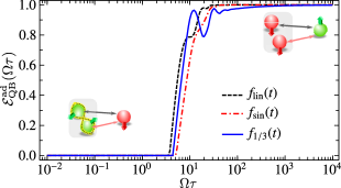
Figure 1: Ergotropy $\mathcal{E}^{\text{ad}}_{\text{{QB}}}(\tau)$ (as a multiple of $\mathcal{E}_{\text{max}}^{\text{qubit}}$) of the QB at the end of the adiabatic evolution (at time $t\!=\!\tau$). Global stability is achieved for $\tau$ at the adiabatic scale.

Each contribution to the Hamiltonian plays a specific role in the energy transfer process. $H_{\text{ini}}$ allows us to encode the state $|\phi(0)\rangle$ as one of its eigenstates. The final desired state $|\phi(\tau_{\text{c}})\rangle$ can then be correctly addressed because it is an eigenstate of $H_{\text{fin}}$ with identical energy and parity as the initial state [14]. Concerning $H_{\text{inter}}$, it is introduced here in order to ensure a non-crossing ground state energy gap.

It is worth mentioning that our choice of the function $f(t)$ may affect the ergotropy transfer rate and the stability of the battery, since the minimum instantaneous gap depends on the function $f(t)$. As an illustration, we will consider three different functions given by $f_{\text{lin}}(t)\!=\!g_{\text{lin}}(t)\!=\!t/\tau$, $f_{\text{sin}}(t)\!=\!g_{\text{sin}}(t)\!=\!\sin\left(\pi t/2\tau\right)$, and $f^{3}_{1/3}(t)\!=\!g_{1/3}(t)\!=\!t/\tau$. The performance of the functions $f(t)$ and $g(t)$ can now be promptly verified. By driving the system by the Hamiltonian $H_{\text{ad}}(t)$ and computing the ergotropy $\mathcal{E}^{\text{ad}}_{\text{{QB}}}(\tau)$ of the QB at the end of the evolution (at time $t\!=\!\tau$), we can analyze the global stability of the energy transfer process. To this end, the Hamiltonian and reduced density matrix used in Eq. (5) are given by $H_{0}^{\text{{QB}}}\!=\!\hbar\omega\sigma_{z}$ and $\rho^{\text{ad}}_{\text{{QB}}}(t)\!=\!\text{Tr}_{{\mathcal{C}}}[\rho_{\text{ad}}(t)]$, respectively. The result is shown in Fig. 1. Notice that, for a given total time $\tau$, the QB ergotropy is approximately equivalent for any interpolation scheme, with some advantage for the linear interpolation in most of regions except the region near $\Omega\tau=10$, where the interpolation via $f_{1/3}(t)$ and $g_{1/3}(t)$ is a better option. Concerning stability, all the three interpolations are globally stable at the adiabatic time scale. In fact, the power of adiabatic chargers is dictated by the energy gap structure of $H_{\text{ad}}(t)$, while its stability is achieved whenever the adiabatic dynamics takes place and the initial state is encoded in a single eigenstate of $H_{\text{ad}}(t)$ [10, 14].

We also consider the instantaneous charge as a function of $t$, for a fixed total time $\tau$. This is performed to study the local stability for different choices of the interpolating functions. Again, the ergotropy is computed for the QB as in Eq. (5). The results are shown in Fig. 2, where we have set $\Omega\tau\!=\!10$. We highlight the intant in which $\Omega t\!=\!10$ (vertical dotted line), so that we can see the efficiency in the stability of each evolution considered. Notice that the interpolation via $f_{1/3}(t)$ and $g_{1/3}(t)$ is able to asymptotically ensure local stability, since it is designed to favor $H_{fin}$ for large $t$. For an always-on connection, this interpolation prevents full backflow of energy from the QB to the charger. From the behavior of the ergotropy, it is straightforward to see that the efficiency $\eta_{\text{ls}}(\Delta t)$ can be drastically affected by the choice of the interpolating function for $H_{\text{ad}}(t)$.

4 Stability of TQD ergotropy transfer

As previously shown, adiabaticity provides an optimal strategy to achieve global stability, even though local stability will depend on the interpolation funtion adopted to drive the system. On the other hand, due to limitations imposed by the validity conditions of adiabatic dynamics, we inevitably have a loss of power in the charging/discharging stage. In order to provide an alternative approach to recover the high-power performance, keeping stability, we will use transitionless quantum driving (TQD) for speeding up the energy transfer process.

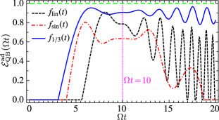
Figure 2: Ergotropy $\mathcal{E}^{\text{ad}}_{\text{{QB}}}(\tau)$ of the QB (as a multiple of $\mathcal{E}_{\text{max}}^{\text{qubit}}$) as a function of $t$, for $\Omega\tau\!=\!10$. The horizontal dashed line denotes the maximal charge, which has been normalized to 1. Local stability strongly depends on the interpolation function adopted.

As originally proposed, the TQD approach for speeding up the adiabatic evolution requires the inclusion of an additional term $H_{\text{cd}}(t)$, called counter-diabatic Hamiltonian, to the original adiabatic Hamiltonian $H_{\text{ad}}(t)$ so that the dynamics is governed by the TQD Hamiltonian $H_{\text{tqd}}(t)=H_{\text{ad}}(t)+H_{\text{cd}}(t)$, where

$$H_{\text{cd}}(t)=i\hbar\sum_{n}|\dot{n}(t)\rangle\langle n(t)|+\langle\dot{n}(t)|n(t)\rangle|n(t)\rangle\langle n(t)|,$$ (12)

with $|n(t)\rangle$ denoting the set of eigenstates of $H_{\text{ad}}(t)$. Under this consideration, one can speed up the adiabatic dynamics by the adiabatic path of $H_{\text{ad}}(t)$, since diabatic transitions are forbidden due to presence of the term $H_{\text{cd}}(t)$. It is known that we can arbitrarily speed up the dynamics, given that the $H_{\text{cd}}(t)$ can be efficiently implemented (or simulated) [18].

In general, the stability of the battery is not a priori guaranteed for TQD even in case where we have perfect control of the time evolution of $H_{\text{tqd}}(t)$. In fact, the stability of the adiabatic approach is obtained because the system state at instant $t\!=\!\tau$ is an eigenstate of $H_{\text{ad}}(t)$, so that the system continuously to evolve to the corresponding instantaneous eigenstate at latter times [14]. Therefore, we do not need to turn off the charger-QB coupling. In the TQD case, due to term $H_{\text{cd}}(t)$, the state of the system at instant $t\!=\!\tau$ is not eigenstate of $H_{\text{tqd}}(t)$, then some dynamics is expected if we do not turn off the charger-QB interaction. However, in cases where we use the boundary conditions to get $H_{\text{cd}}(t\!=\!0)\!=\!H_{\text{cd}}(t\!=\!\tau)\!=\!0$, the stability is recovered. It is known that such boundary condition can be obtained for a number of evolutions [37, 38, 26], but here we will adopt a milder assumption, with no boundary conditions on time taken. As we shall see, even under this assumption, we get considerable degree of stability while speeding up the ergotropy transfer process.

To study the performance of TQD charging, we consider the shortcut to the adiabatic evolution driven by the Hamiltonian in Eq. (8). First, let us consider global stability. To this end, given the counter-diabatic term $H_{\text{cd}}(t)$, we let the charger-QB evolve under $H_{\text{tqd}}(t)$ and then we compute the QB ergotropy at $t\!=\!\tau$. In Fig. 3 we show the ergotropy $\mathcal{E}^{\text{tqd}}_{\text{{QB}}}(\tau)$ of the QB after the TQD evolution, where we choose two different interpolations, namely, $f_{\text{lin}}(t)$ and $f_{1/3}(t)$ to get a comparison between the adiabatic and TQD charging performance. While adiabatic charging requires a specific minimum time $\tau$ to achieve maximum charge (or to get some non-zero amount of ergotropy), the counter-diabatic energy transfer leads to a maximum charge state at an arbitrary time interval. This is a consequence of the inverse engineering approach, where a suitable counter-diabatic contribution allows us to mimic the adiabatic dynamics at arbitrary $\tau$, as dictated by the quantum speed limit for counter-diabatic dynamics [18]. On the other hand, it is worth highlighting that such additional advantage comes at the well-known cost of some intensity-field demand in the term $H_{\text{cd}}(t)$ in $H_{\text{tqd}}(t)$ [18].

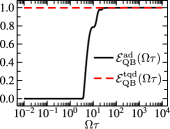
(a) $f_{\text{lin}}(t)$

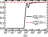
(b) $f_{1/3}(t)$

Figure 3: Adiabatic and TQD ergotropy transfer from the charger to the QB (as a multiple of $\mathcal{E}_{\text{max}}^{\text{qubit}}$) at instant $t\!=\!\tau$, as a function of $\Omega\tau$, for distinct interpolation functions, namely, $f_{\text{lin}}(t)$ [Fig. (3a)] and $f_{1/3}(t)$ [Fig. (3b)].

Concerning local stability, we can also show that the conter-diabatic approach provides a robust charge method even if fluctuations of the total time $\tau$ are taken into account. This is illustrated in Fig. 4, where both adiabatic and TQD ergotropy transfer from the charger to the QB (as a multiple of $\mathcal{E}_{\text{max}}$) are plotted as a function of $\Omega t$ for different total times $\tau$ and for the interpolation function given by $f_{1/3}(t)$ e $g_{1/3}(t)$. Notice that, by adopting $\Omega\tau=1$, the adiabatic condition is violated. Again, we highlight the instant $\Omega t\!=\!1$ as a vertical dotted line. In that case, the TQD approach is still able to mimic adiabaticity and to provide a locally stable ergotropy transfer. Even though we have the local stability coefficient $\eta_{\textrm{ls}}>0$, the QB ergotropy is kept in a large value in the asymptotic regime. In the inset of Fig. 4, we also consider a case of validity of adiabaticity by setting $\Omega\tau=10$ (vertical dotted line denotes the instant $\Omega t\!=\!10$). In this situation, both the adiabatic method and the TQD approach provide a locally stable charging process from the charger to the QB.

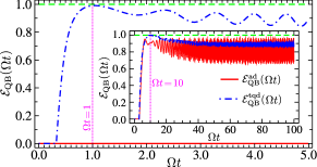
Figure 4: Adiabatic and TQD ergotropy transfer from the charger to the QB (as a multiple of $\mathcal{E}_{\text{max}}^{\text{qubit}}$) as a function of $\Omega t$, for the interpolation function given by $f_{1/3}(t)$ e $g_{1/3}(t)$. The ergotropy is shown for the case of $\Omega\tau=1$, where the TQD approach is able to provide a stable charge, while the adiabatic method fails. The horizontal dashed line denotes the maximal charge, which has been normalized to 1. In the inset, a slower evolution is adopted by setting $\Omega\tau\!=\!10$, so that both TQD and adiabatic dynamics achieve local stability.

5 Energy cost of the charging process

In this section we briefly discuss the external energy cost of implementing the TQD charging process in comparison with the adiabatic evolution. It is known that the standard approach of TQD is more energetically costly than its adiabatic counterpart [18]. However, as we shall see, it is possible to find a range of values of the total evolution time for which the TQD charging provides a beneficial setup. To this end, let us consider the measure $\Sigma(\tau)$ of energy cost for implementing a time-dependent Hamiltonian through the interval $t\in[0,\tau]$, which is provided by

$$\Sigma(\tau)=\frac{1}{\tau}\int_{0}^{\tau}||H(t)||_{\text{HS}}dt,$$ (13)

where $||A||_{\text{HS}}\!=\!(\text{Tr}\left\{AA^{\dagger}\right\})^{1/2}$ is the Hilbert-Schmidt norm of the operator $A$. We observe that $\Sigma(\tau)$ has been used in experimental implementations of TQD in order to quantify the energy cost of simulating adiabatic and TQD evolutions [39, 40]. Moreover, it has recently been shown in Ref. [41] that this quantity allows for quantifying the thermodynamic cost of implementing the dynamics driven by an arbitrary Hamiltonian $H(t)$. By explicitly evaluating the adiabatic and TQD energy costs, we then obtain

$$\Sigma_{\text{ad}} =\frac{1}{\tau}\int_{0}^{\tau}||H_{\text{ad}}(t)||_{\text{HS}}dt=\frac{1}{\tau}\int_{0}^{\tau}\sqrt{\sum_{n}E_{n}^{2}(t)}dt,$$ (14)

$$\Sigma_{\text{tqd}} =\frac{1}{\tau}\int_{0}^{\tau}||H_{\text{tqd}}(t)||_{\text{HS}}dt$$

$$=\frac{1}{\tau}\int_{0}^{\tau}\sqrt{\sum_{n}E_{n}^{2}(t)+\hbar^{2}\mu_{n}(t)}dt,$$

where $\mu_{n}(t)=\langle\dot{n}(t)|\dot{n}(t)\rangle-|\langle n(t)|\dot{n}(t)\rangle|^{2}$ [19]. Therefore, given the parameters $\Omega$ and $\tau$, and the functions $f(t)$ and $g(t)$, the quantities above can be directly computed. In our case, we consider the linear function $f_{\text{lin}}(t)$ and perform the integration by numerical methods, with results shown in Fig. 5. It is also convenient to define the ratio $\Sigma_{\text{rel}}=\Sigma_{\text{tqd}}/\Sigma_{\text{ad}}$, which quantifies how larger the energy cost is in the TQD dynamics in comparison with its adiabatic counterpart. The result for $\Sigma_{\text{rel}}$ is shown in the inset of Fig. 5.

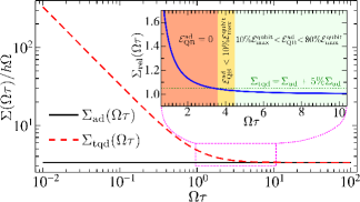
Figure 5: Energy cost (as a multiple of $\hbar\Omega$) as a function of $\Omega\tau$ for the implementation of the adiabatic and TQD charging of the QB. Inset: The relative cost of the TQD process in comparison with the adiabatic charging. Here we consider the interpolation function $f_{\text{lin}}(t)$.

As expected, the faster the charging process is, the larger the energy cost to implement it in a TQD process, as we can see in Fig. 5. However, it is possible to find a range of values for the charging time $\tau$ for which the TQD protocol presents better performance with respect to the adiabatic case. In fact, in the inset of Fig. 5, we consider the time interval between $\Omega\tau$ and $10\Omega\tau$. As previously shown in Fig. 3a, for this interval, the TQD process allows us for reaching the full charged state of the battery, while the adiabatic evolution cannot charge the battery efficiently ( with the maximum being around $80\%$ of $\mathcal{E}_{\text{max}}^{\text{qubit}}$). Then, by taking into account the cost of implementing the transitionless evolution, relatively to the adiabatic dynamics, it is worth supporting the charging process via TQD. For example, consider the range of values where $\mathcal{E}^{\text{ad}}_{\text{QB}}<10\%\mathcal{E}_{\text{max}}^{\text{qubit}}$, as highlighted in the yellow box in Fig. 5 (inset). For this interval of values for $\Omega\tau$, the maximum value for $\Sigma_{\text{tqd}}(\Omega\tau)$ corresponds to a mild TQD increasing cost, with $\Sigma_{\text{tqd}}\!=\Sigma_{\text{ad}}+\!5\%\Sigma_{\text{ad}}$.

6 Conclusion

We have proposed a solution for the local stability of QBs as well as for the inherent control of their charging power. This allows for the implementations of always-on chargers that are able to charge a QB as fast as the energy available for their internal dynamics. The charger-QB model proposed here is composed by a set of independent three-qubit cells, which ensures the locality of the interaction Hamiltonian. The energy resources can be further optimized by implementing a more general approach of TQD technique [42]. In this approach, the phase accompanying the state vector that mimics the adiabatic evolution is set as a free parameter that can be used to adjust the interaction Hamiltonian for a smoother TQD energy requirement. This is a certainly interesting point for further analysis. Moreover, it is also potentially fruitful the investigation of the relationship between the correlations present in the charger and its performance with respect to the energy storage and transfer. This may bring insights about possible generalizations of the charger model to favor the relevant correlations. These topics are left for future research.

It is worth mentioning that we recently became aware of a work in which the authors also consider TQD for speeding up the adiabatic charging process of three-level quantum batteries [43].

- [1] \NameAlicki R. Fannes M. \REVIEWPhys. Rev. E872013042123.
- [2] \NameHovhannisyan K. V., Perarnau-Llobet M., Huber M. Acín A. \REVIEWPhys. Rev. Lett.1112013240401.
- [3] \NameCampaioli F., Pollock F. A., Binder F. C., Céleri L., Goold J., Vinjanampathy S. Modi K. \REVIEWPhys. Rev. Lett.1182017150601.
- [4] \NameAndolina G. M., Keck M., Mari A., Campisi M., Giovannetti V. Polini M. \REVIEWPhys. Rev. Lett.1222019047702.
- [5] \NameLe T. P., Levinsen J., Modi K., Parish M. M. Pollock F. A. \REVIEWPhys. Rev. A972018022106.
- [6] \NameBinder F. C., Vinjanampathy S., Modi K. Goold J. \REVIEWNew J. Phys.172015075015.
- [7] \NameFusco L., Paternostro M. De Chiara G. \REVIEWPhys. Rev. E942016052122.
- [8] \NameZhang Y.-Y., Yang T.-R., Fu L. Wang X. \REVIEWPhys. Rev. E992019052106.
- [9] \NameFerraro D., Campisi M., Andolina G. M., Pellegrini V. Polini M. \REVIEWPhys. Rev. Lett.1202018117702.
- [10] \NameSantos A. C., Çakmak B., Campbell S. Zinner N. T. \REVIEWPhys. Rev. E1002019032107.
- [11] \NameAndolina G. M., Farina D., Mari A., Pellegrini V., Giovannetti V. Polini M. \REVIEWPhys. Rev. B982018205423.
- [12] \NameAndolina G. M., Keck M., Mari A., Giovannetti V. Polini M. \REVIEWPhys. Rev. B992019205437.
- [13] \NameLong W., Sun Q.-F., Guo H. Wang J. \REVIEWAppl. Phys. Lett.8320031397.
- [14] \NameSantos A. C., Saguia A. Sarandy M. S. \REVIEWPhys. Rev. E1012020062114.
- [15] \NameDemirplak M. Rice S. A. \REVIEWJ. Phys. Chem. A10720039937.
- [16] \NameDemirplak M. Rice S. A. \REVIEWJ. Phys. Chem. B10920056838.
- [17] \NameBerry M. \REVIEWJ. Phys. A: Math. Theor.422009365303.
- [18] \NameSantos A. C. Sarandy M. S. \REVIEWSci. Rep.5201515775.
- [19] \NameSantos A. C., Silva R. D. Sarandy M. S. \REVIEWPhys. Rev. A932016012311.
- [20] \NameCoulamy I. B., Santos A. C., Hen I. Sarandy M. S. \REVIEWFrontiers in ICT3201619.
- [21] \NameHegade N. N., Paul K., Ding Y., Sanz M., Albarrán-Arriagada F., Solano E. Chen X. \REVIEWPhys. Rev. Applied152021024038.
- [22] \NameBeau M., Jaramillo J. del Campo A. \REVIEWEntropy182016168.
- [23] \NameHerrera M., Sarandy M. S., Duzzioni E. I. Serra R. M. \REVIEWPhys. Rev. A892014022323.
- [24] \NameChen Z., Chen Y., Xia Y., Song J. Huang B. \REVIEWSci. Rep.6201622202.
- [25] \NameChen X., Lizuain I., Ruschhaupt A., Guéry-Odelin D. Muga J. G. \REVIEWPhys. Rev. Lett.1052010123003.
- [26] \NameGuéry-Odelin D., Ruschhaupt A., Kiely A., Torrontegui E., Martínez-Garaot S. Muga J. G. \REVIEWRev. Mod. Phys.912019045001.
- [27] \NameAllahverdyan A. E., Balian R. Nieuwenhuizen T. M. \REVIEWEurophys. Lett.672004565.
- [28] \NameÇakmak B. \REVIEWPhys. Rev. E1022020042111.
- [29] \NameKamian F. H., Tabesh F. T., Salimi S., Kheirandish F. Santos A. C. \REVIEWNew J. Phys.222020083007.
- [30] \NameQuach J. Q. Munro W. J. \REVIEWPhys. Rev. Applied142020024092.
- [31] \NameBocchieri P. Loinger A. \REVIEWPhys. Rev.1071957337.
- [32] \NameBorn M. Fock V. \REVIEWZeitschrift für Physik A Hadrons and Nuclei511928165.
- [33] \NameKato T. \REVIEWJournal of the Physical Society of Japan51950435.
- [34] \NameMessiah A. \BookQuantum Mechanics Quantum Mechanics (North-Holland Publishing Company) 1962.
- [35] \NameSarandy M. S., Wu L.-A. Lidar D. A. \REVIEWQuantum Information Processing32004331.
- [36] \NameBai S.-Y. An J.-H. \REVIEWPhys. Rev. A1022020060201.
- [37] \NameIbáñez S., Chen X., Torrontegui E., Muga J. G. Ruschhaupt A. \REVIEWPhys. Rev. Lett.1092012100403.
- [38] \NameTorrontegui E., Ibáñez S., Martínez-Garaot S., Modugno M., del Campo A., Guéry-Odelin D., Ruschhaupt A., Chen X. Muga J. G. \BookChapter 2 - shortcuts to adiabaticity in \BookAdvances in Atomic, Molecular, and Optical Physics, edited by \NameArimondo E., Berman P. R. Lin C. C. Vol. 62 of Advances In Atomic, Molecular, and Optical Physics (Academic Press) 2013 pp. 117 – 169.
- [39] \NameSantos A. C., Nicotina A., Souza A. M., Sarthour R. S., Oliveira I. S. Sarandy M. S. \REVIEWEPL (Europhysics Letters)129202030008.
- [40] \NameHu C.-K., Cui J.-M., Santos A. C., Huang Y.-F., Sarandy M. S., Li C.-F. Guo G.-C. \REVIEWOpt. Lett.4320183136.
- [41] \NameDeffner S. \REVIEWarXiv e-prints2021arXiv:2102.05118.
- [42] \NameSantos A. C. Sarandy M. S. \REVIEWJ. Phys. A: Math. Theor.512018025301.
- [43] \NameHu H., Qi S. Jing J. \REVIEWarXiv e-prints2021arXiv:2104.12143.