Semi-supervised novelty detection using
ensembles with regularized disagreement

Abstract

Deep neural networks often predict samples with high confidence even when they come from unseen classes and should instead be flagged for expert evaluation. Current novelty detection algorithms cannot reliably identify such near OOD points unless they have access to labeled data that is similar to these novel samples. In this paper, we develop a new ensemble-based procedure for semi-supervised novelty detection (SSND) that successfully leverages a mixture of unlabeled ID and novel-class samples to achieve good detection performance. In particular, we show how to achieve disagreement only on OOD data using early stopping regularization. While we prove this fact for a simple data distribution, our extensive experiments suggest that it holds true for more complex scenarios: our approach significantly outperforms state-of-the-art SSND methods on standard image data sets (SVHN/CIFAR-10/CIFAR-100) and medical image data sets with only a negligible increase in computation cost.

1 Introduction

Despite achieving great in-distribution (ID) prediction performance, deep neural networks (DNN) often have trouble dealing with test samples that are out-of-distribution (OOD), i.e. test inputs that are unlike the data seen during training. In particular, DNNs often make incorrect predictions with high confidence when new unseen classes emerge over time (e.g. undiscovered bacteria [41], new diseases [22]). Instead, we would like to automatically detect such novel samples and bring them to the attention of human experts.

Figure 1: Novelty detection is challenging since X-rays of novel diseases are remarkably similar to known conditions. The unlabeled batch of inference-time data can be used to adapt a semi-supervised novelty detection approach to emerging novel diseases.

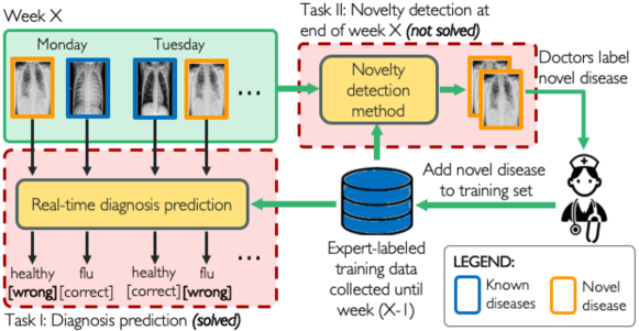
Consider, for instance, a hospital with a severe shortage of qualified personnel. To make up for the lack of doctors, the hospital would like to use an automated system for real-time diagnosis from X-ray images (Task I) and a novelty detection system, which can run at the end of each week, to detect outbreaks of novel disease variants (Task II) (see Figure 1). In particular, the detection algorithm can be fine-tuned weekly with the unlabeled batch of data collected during the respective week.

While the experts are examining the peculiar X-rays over the course of the next week, the novelty detection model helps to collect more instances of the same new condition and can request human review for these patients. The human experts can then label these images and include them in the labeled training set to update both the diagnostic prediction and the novelty detection systems. This process repeats each week and enables both diagnostic and novelty detection models to adjust to new emerging diseases.

Note that, in this example, the novelties are a particular kind of out-of-distribution samples with two properties. First, several novel-class samples may appear in the unlabeled batch at the end of a week, e.g. a contagious disease will lead to several people in a small area to be infected. This situation is different from cases when outliers are assumed to be singular, e.g. anomaly detection problems. Second, the novel-class samples share many features in common with the ID data, and only differ from known classes in certain minute details. For instance, both ID and OOD samples are frontal chest X-rays, with the OOD samples showing distinctive signs of a pneumonia caused by a new virus. In what follows, we use the terms novelty detection and OOD samples to refer to data with these characteristics.

Automated diagnostic prediction systems (Task I) can already often have satisfactory performance [5]. In contrast, novelty detection (Task II) still poses a challenging problem in these scenarios. Many prior approaches can be used for semi-supervised novelty detection (SSND), when a batch of unlabeled data that may contain OOD samples is available, like in Figure 1. However, all of these methods fail to detect novel-class data when used with complex models, like neural networks.

Figure 2: Left: Sketch of the SSND setting. Middle and Right: Novelty detection with a diverse ensemble.

Despite showing great success on simple benchmarks like SVHN vs CIFAR10, SOTA unsupervised OOD detection methods perform poorly on near OOD data [51] where OOD inputs are similar to the training samples. Furthermore, even though unlabeled data can benefit novelty detection scott09 [45], existing SSND methods for deep neural networks [24, 15, 57, 54] cannot improve upon unsupervised methods on near OOD data sets. Even methods that violate fundamental OOD detection assumptions by using known test OOD data for hyperparameter tuning [30, 28, 54] fail to work on challenging novelty detection tasks. Finally, large pretrained models seem to solve near OOD detection [11], but they only work for extremely specific OOD data sets (see Section 5 for details).

This situation naturally raises the following question:

Can we improve semi-supervised novelty detection for neural networks?

In this paper, we introduce a new method that successfully leverages unlabeled data to obtain diverse ensembles for novelty detection. Our contributions are as follows:

• We propose to find Ensembles with Regularized Disagreement (ERD), that is, disagreement only on OOD data. Our algorithm produces ensembles just diverse enough to be used for novelty detection with a disagreement test statistic (Section 2).

• We prove that training with early stopping leads to regularized disagreement, for data that satisfies certain simplifying assumptions (Section 3).

• We show experimentally that ERD significantly outperforms existing methods on novelty detection tasks derived from standard image data sets, as well as on medical image benchmarks (Section 4).

2 Proposed method

Input : Train set $S$, Validation set $V$, Unlabeled set $U$, Model $\tilde{f}$ pretrained on $S$, Ensemble size $K$

Result: ERD ensemble $\{f_{y_{i}}\}_{i=1}^{K}$

Sample $K$ different labels $\{y_{1},...,y_{K}\}$ from $\mathcal{Y}$

for $c\leftarrow\{y_{1},...,y_{K}\}$ do // fine-tune $K$ models

       $f_{c}\leftarrow\textit{Initialize}(\tilde{f})$

       $(U,c)\leftarrow\{(x,c):x\in U\}$

       $f_{c}\leftarrow\textit{EarlyStoppedFineTuning}\left(f_{c},S\cup(U,c);V\right)$

      

return $\{f_{y_{i}}\}_{i=1}^{K}$

Algorithm 1 Obtaining ERD ensemble via early stopping

Input : Ensemble $\{f_{y_{i}}\}_{i=1}^{K}$, Test set $T$, $O=\emptyset$, Threshold $t_{0}$, Disagreement metric $\rho$

Result: $O$, i.e. the novel-class samples from $T$

for $x\in T$ do // run hypothesis test

       if $(\text{Avg}\circ\rho)(f_{y_{1}},...,f_{y_{K}})(x)>t_{0}$ then

             $O\leftarrow O\cup\{x\}$

            

      

return $O$

Algorithm 2 Novelty detection using ERD

In this section we first introduce our proposed method to obtain Ensembles with Regularized Disagreement (ERD) and describe how they can be used for novelty detection.

2.1 Training ensembles with regularized disagreement (ERD)

Recall from Figure 1 that we have access to both a labeled training set $S=\{(x_{i},y_{i})\}_{i=1}^{n}\sim P$, with covariates $x_{i}\in\mathcal{X}_{ID}$ and discrete labels $y_{i}\in\mathcal{Y}$, and an unlabeled set $U$, which contains both ID and unknown OOD samples. Moreover, we initialize the models of the ensemble using the weights of a predictor with good in-distribution performance, pretrained on $S$. In the scenarios we consider, such a well-performing pretrained classifier is readily available, as it solves Task I in Figure 1.

The entire training procedure is described in Algorithm 1. For training a single model in the ensemble, we assign a label $c\in\mathcal{Y}$ to all the unlabeled points in $U$, resulting in the $c$-labeled set that we denote as $(U,c):=\{(x,c):x\in U\}$. We then fine-tune a classifier $f_{c}$ on the union $S\cup(U,c)$ of the correctly-labeled training set $S$, and the unlabeled set $(U,c)$. In particular, we choose an early stopping time at which validation accuracy is high and training error on $S\cup(U,c)$ is low. We create a diverse ensemble of $K$ classifiers $f_{c}$ by choosing a different artificial label $c\in\mathcal{Y}$ for every model.

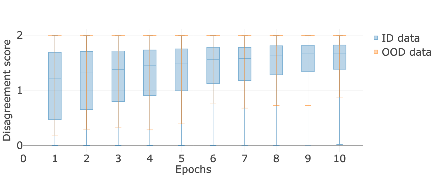
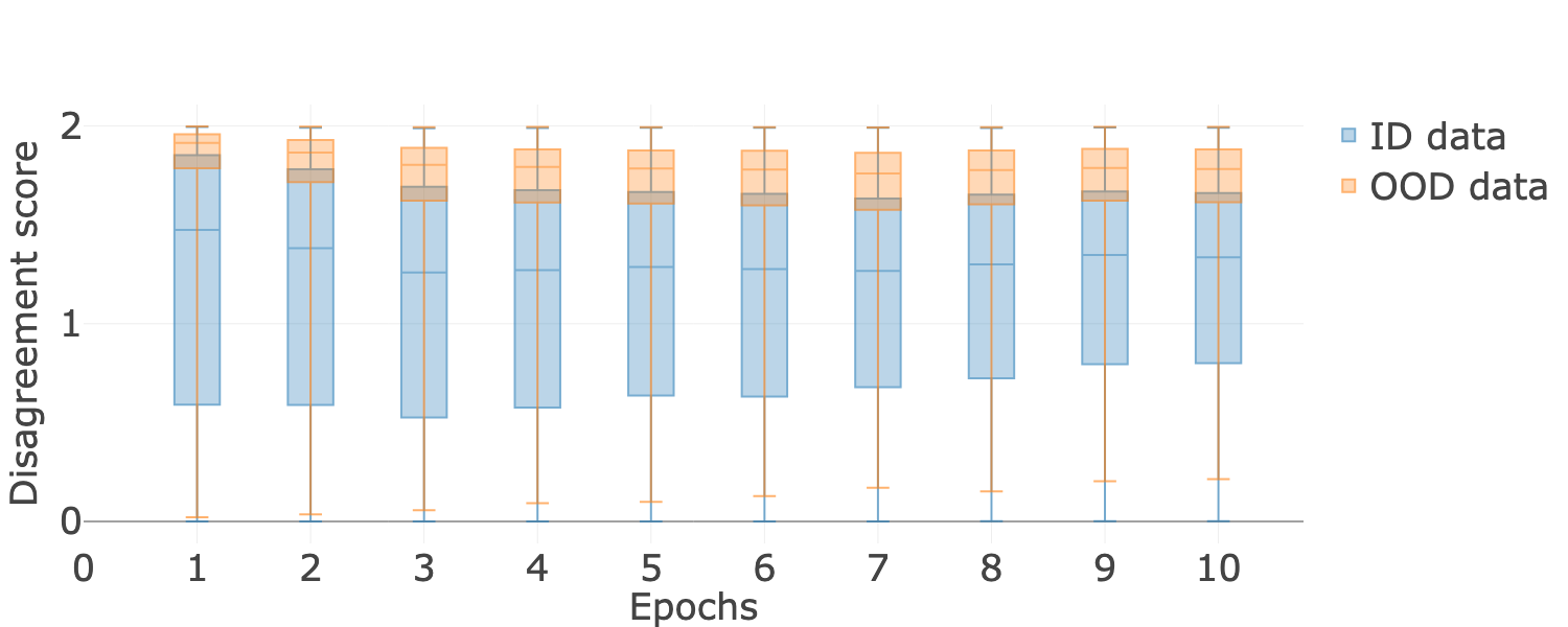
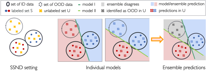
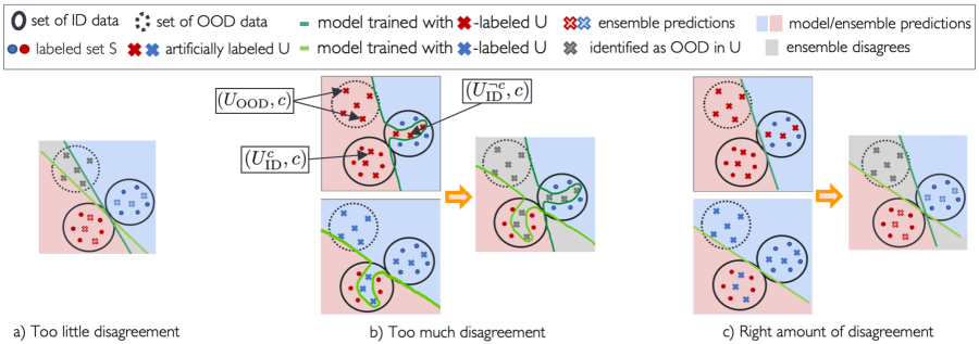
Intuitively, encouraging each model in the ensemble to fit different labels to the unlabeled set $U$ promotes disagreement, as shown in Figure 2. In the next sections, we elaborate on how to use diverse ensembles for novelty detection.

2.2 Ensemble disagreement for novelty detection

We now discuss how we can use ensembles with disagreement to detect OOD samples and why the right amount of diversity is crucial. Note that we can cast the novelty detection problem as a hypothesis test with the null hypothesis $H_{0}:x\in\mathcal{X}_{ID}$.

As usual, we test the null hypothesis by comparing a test statistic with a threshold $t_{0}$: The null hypothesis is rejected and we report $x$ as OOD (positive) if the test statistic is larger than $t_{0}$ (Section 4.3 elaborates on the choice of $t_{0}$). In particular, we use as test statistic the following disagreement score, which computes the average distance between the softmax outputs of the $K$ models in the ensemble:

$$(\text{Avg}\circ\rho)(f_{1}(x),...,f_{K}(x)):=\frac{2\sum_{i\neq j}\rho\left(f_{i}(x),f_{j}(x)\right)}{K(K-1)},$$

where $\rho$ is a measure of disagreement between the softmax outputs of two predictors, for example the total variation distance $\rho_{\text{TV}}(f_{i}(x),f_{j}(x))=\frac{1}{2}\|f_{i}(x)-f_{j}(x)\|_{1}$ used in our experiments. We provide a thorough discussion on the soundness of this test statistic for disagreeing models and compare it with previous metrics in Appendix B.

Even though previous work like mcd_ood [54] used a similar disagreement score, their detection performance is notably worse. The reason lies in the lack of diversity in their trained ensemble (see Figure 8(a) in Appendix B). On the other hand Algorithm 1 without early stopping would lead to a too diverse ensemble, that also disagrees on ID points, and hence, has a high false positive rate (see Appendix K). In the next section, we explain why novelty detection with this test statistic crucially relies on the right amount of ensemble diversity and how ensembles may achieve this goal if they are trained to have regularized disagreement.

Figure 3: a) Ensembles with too little disagreement fail to detect OOD samples. b) An ensemble of two models trained on $S\cup(U,c)$ disagrees on both ID and OOD data. b) Regularization prevents models from fitting $(U_{\mathrm{ID}}^{\neg c},c)$, limiting disagreement to only OOD samples.

2.3 Desired ensemble diversity via regularized disagreement

For simplicity of illustration, let us first assume a training set with binary labels and a semi-supervised novelty detection setting as depicted in Figure 2 a). For an ensemble with two models, like in Figure 2 b), the model predictions agree on the blue and red areas and disagree on the gray area depicted in Figure 2 c). Note that the two models in Figure 2 are just diverse enough to obtain both high power (flag true OOD as OOD) and low false positive rate (avoid flagging true ID as OOD) at the same time.

Previous methods that try to leverage unlabeled data to obtain more diverse ensembles either do not work with deep neural networks [3, 56, 21] or do not disagree enough on OOD data [54], leading to subpar novelty detection performance (see Figure 8(a) in Appendix B).

To obtain the right amount of diversity, it is crucial to train ensembles with regularized disagreement on the unlabeled set: The models should disagree on the unlabeled OOD samples, but agree on the unlabeled ID points (Figure 3c). Thus, we avoid having too little disagreement as in Figure 3a), which results in low power, or too much diversity, resulting in high false positive rate as in Figure 3b). In particular, if models $f_{c}$ predict the correct label on ID points and the label $c$ on OOD data, we can effectively use disagreement to detect novel-class samples. Since classifiers with good ID generalization need to be smooth, we expect the model predictions on holdout OOD data from the same distributions to be in line with the predictions on the unlabeled set.

In Section 3 we argue that the training procedure in Algorithm 1 successfully induces regularized disagreement and prove it in a synthetic setting. Our experiments in Section 4 further corroborate our theoretical statements. Finally, we note that one could also use other regularization techniques like dropout or weight decay. However, running a grid search to select the right hyperparameters can be more computationally expensive than simply using one run of the training process to select the optimal stopping time.

3 Provable regularized disagreement via early stopping

In this section, we show how using early stopping in Algorithm 1 prevents fitting the incorrect artificial label on the unlabeled ID samples. Albeit for a simplified setting, this result provides a rigorous proof of concept and intuition for why ERD ensembles achieve the right amount of diversity necessary for good novelty detection.

3.1 Preliminary definitions

We first introduce necessary definitions to prepare the mathematical statement. Recall that in our approach, in addition to the correct labels of the ID training set $S$, each member of the ensemble tries to fit one label $c$ to the entire unlabeled set $U$ that can be further partitioned into

$$(U,c) =(U_{\mathrm{ID}},c)\cup(U_{\mathrm{OOD}},c)$$

$$=\{(x,c):x\in U_{\mathrm{ID}}\}\cup\{(x,c):x\in U_{\mathrm{OOD}}\},$$

where $U_{\mathrm{ID}}:=U\cap\mathcal{X}_{ID}$ and $U_{\mathrm{OOD}}:=U\setminus U_{\mathrm{ID}}$. Moreover, assuming that the label of an ID input $x$ is deterministically given by $y^{*}(x)$, we can partition the set $(U_{\mathrm{ID}},c)$ (see Figure 3b) into a subset of effectively “correctly labeled” samples $(U_{\mathrm{ID}}^{c},c)$ and “incorrectly labeled” samples $(U_{\mathrm{ID}}^{\neg c},c)$:

$$(U_{\mathrm{ID}}^{\neg c},c):=\{(x,c):x\in U_{\mathrm{ID}}\text{ with }y^{*}(x)\neq c\}$$

$$(U_{\mathrm{ID}}^{c},c):=\{(x,c):x\in U_{\mathrm{ID}}\text{ with }y^{*}(x)=c\}.$$

Note that $(U_{\mathrm{ID}}^{\neg c},c)$ can be viewed as the subset of noisy samples from the entire training set $S\cup(U,c)$.

3.2 Main result

We now prove that there exists indeed an optimal stopping time at which a two-layer neural network trained with gradient descent does not fit the incorrectly labeled subset $(U_{\mathrm{ID}}^{\neg c},c)$, under mild distributional assumptions.

For the formal statement, we assume that the artificially labeled set $S\cup(U,c)$ is clusterable, i.e. the points can be grouped in $K$ clusters of similar sizes. Each class may comprise several clusters, but every cluster contains only samples from one class. Any cluster may include at most a fraction $\rho\in[0,1]$ of samples with label noise, e.g. $(U_{\mathrm{ID}}^{\neg c},c)$. We denote by $c_{1},...,c_{K}$ the cluster centers and define the matrix $C:=[c_{1},...,c_{K}]^{T}\in\mathbb{R}^{K\times d}$. Further, let $\lambda_{C}^{NN}$ be a measure of how well a two-layer neural network can separate the cluster centers ($\lambda_{C}^{NN}=0$ if $c_{i}=c_{j}$ for some $i,j\leq K$). Under these assumptions we have the following:

Proposition 3.1.

(informal) It holds with high probability over the initialization of the weights that a two-layer neural network trained on $S\cup(U,c)$ perfectly fits $S$, $(U_{\mathrm{ID}}^{c},c)$ and $(U_{\mathrm{OOD}},c)$, but not $(U_{\mathrm{ID}}^{\neg c},c)$, after $T\simeq\frac{\|C\|^{2}}{\lambda_{C}^{NN}}$ iterations.

The precise assumptions for the proposition can be found in Appendix A. On a high level, the reasoning follows from two simple insights: 1. When the artificial label is not equal to the true label, the ID samples in the unlabeled set can be seen as noisy samples in the set $S\cup(U,c)$. 2. It is well known that early stopping prevents models from fitting incorrect labels since noisy samples with incorrect labels are often fit later during training (see e.g. theoretical and empirical evidence here [53, 29, 49, 33]). In particular, our proof heavily relies on Theorem 2.2 of mahdi [29] which shows that early stopped predictors are robust to label noise.

Proposition 3.1 gives a flavor of the theoretical guarantees that ERD enjoys. Albeit simple, the clusterable data model actually includes data with non-linear decision boundaries. On the other hand, the requirement that the clusters are balanced seems rather restrictive. In our experiments we show that this condition is in fact more stringent than it should. In particular, our method still works when the number of OOD samples $|U_{\mathrm{OOD}}|$ is considerably smaller than the number of ID samples from any given class, as we show in Section 4.5.

3.3 Choosing the early stopping time

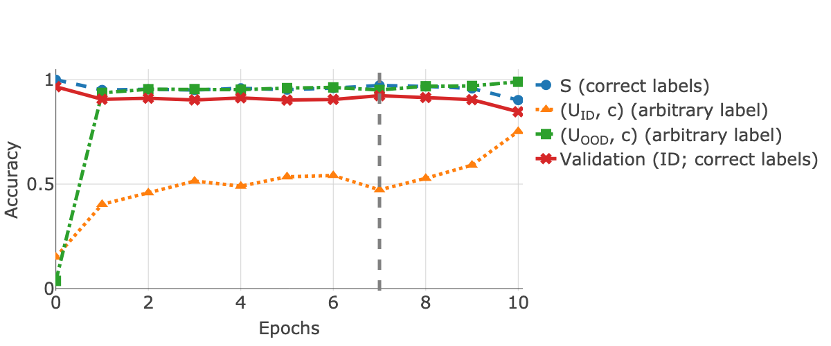
In practice, we avoid computing the exact value of $T$ by using instead a heuristic for picking the early stopping iteration with the highest validation accuracy (indicated by the vertical line in Figure 4). As shown in the figure, the model fits the noisy training points, i.e. $(U_{\mathrm{ID}}^{\neg c},c)$, late during fine-tuning, which causes the validation accuracy to decrease, since the model will also predict the incorrect label $c$ on some validation ID samples. In Appendix J we show that the trend in Figure 4 is consistent across data sets.

Figure 4: Accuracy during fine-tuning a model pretrained on $S$ (epoch 0 indicates values obtained with the initial pretrained weights). The samples in $(U_{\mathrm{OOD}},c)$ are fit first, while the model reaches high accuracy on $(U_{\mathrm{ID}},c)$ much later. We fine-tune for at least one epoch and then early stop when the validation accuracy starts decreasing after 7 epochs (vertical line). The model is trained on SVHN[0:4] as ID and SVHN[5:9] as OOD.

4 Experimental results

In this section we evaluate the novelty detection performance of ERD with deep neural networks on several image data sets. On difficult near OOD data sets, we find that our approach outperforms all baselines, including SSND methods, but also methods operating in other, sometimes more favorable settings. In addition, we discuss some of the trade-offs that impact ERD’s performance.

4.1 Data sets

Our experiments focus on novel-class detection scenarios where the ID and OOD data share many similar features and only differ in a few characteristics. We use standard image data sets (e.g. CIFAR10/CIFAR100) and consider half of the classes as ID, and the other half as novel. We also assess ERD’s performance on a medical image benchmark [6], where near OOD data consists of novel unseen diseases (e.g. X-rays of the same body part from patients with different conditions; see Appendix E for details). Further, we also include far OOD data sets (e.g. CIFAR10/CIFAR100 vs SVHN) for completeness.

For all scenarios, we used a labeled training set (e.g. 40K samples for CIFAR10), a validation set with ID samples (e.g. 10K samples for CIFAR10) and an unlabeled test set where half of the samples are ID and the other half are OOD (e.g. 5K ID samples and 5K OOD samples for CIFAR10 vs SVHN). For evaluation, we use a holdout set containing ID and OOD samples in the same proportions as the unlabeled set. Moreover, in Appendix F.5 we present results obtained with a smaller unlabeled set of only 1K samples.

Table 1: AUROC and TNR@95 for ERD and various baselines (we highlight the best baseline). Numbers in square brackets indicate the ID/OOD classes. Asterisks mark methods proposed in this paper. Mahal, nnPU and MCD (^†) use oracle information about the OOD data. Repeated runs of ERD show a small variance $\sigma^{2}<0.01$ in the detection metrics.

		Other settings					SSND
ID data	OOD data	Vanilla Ensembles	Gram	DPN	OE	Mahal.†	nnPU†	MCD†	Mahal-U	Bin. Classif. *	ERD *
		AUROC $\uparrow$ / TNR@95 $\uparrow$
SVHN	CIFAR10	0.97 / 0.88	0.97 / 0.86	1.00 / 1.00	1.00 / 1.00	0.99 / 0.98	1.00 / 1.00	0.97 / 0.85	0.99 / 0.95	1.00 / 1.00	0.99 / 0.98
CIFAR10	SVHN	0.92 / 0.78	1.00 / 0.98	0.95 / 0.85	0.97 / 0.89	0.99 / 0.96	1.00 / 1.00	1.00 / 0.98	0.99 / 0.96	1.00 / 1.00	1.00 / 1.00
CIFAR100	SVHN	0.84 / 0.48	0.99 / 0.97	0.77 / 0.44	0.82 / 0.50	0.98 / 0.90	1.00 / 1.00	0.97 / 0.73	0.98 / 0.92	1.00 / 1.00	1.00 / 1.00
SVHN [0:4]	SVHN [5:9]	0.92 / 0.69	0.81 / 0.31	0.87 / 0.19	0.85 / 0.52	0.92 / 0.71	0.96 / 0.73	0.91 / 0.51	0.91 / 0.63	0.81 / 0.40	0.95 / 0.73
CIFAR10 [0:4]	CIFAR10 [5:9]	0.80 / 0.39	0.67 / 0.15	0.82 / 0.32	0.82 / 0.41	0.79 / 0.27	0.61 / 0.11	0.69 / 0.25	0.64 / 0.13	0.85 / 0.43	0.89 / 0.57
CIFAR100 [0:49]	CIFAR100 [50:99]	0.78 / 0.35	0.71 / 0.16	0.70 / 0.26	0.74 / 0.31	0.72 / 0.20	0.53 / 0.06	0.70 / 0.26	0.72 / 0.19	0.66 / 0.13	0.81 / 0.41

4.2 Baselines

We compare our method against a wide range of baselines that are applicable in the SSND setting.

Semi-supervised novelty detection.

We primarily compare ERD to SSND approaches that are designed to incorporate a small set of unlabeled ID and novel samples.

The MCD method [54] trains an ensemble of two classifiers such that one model gives high-entropy and the other yields low entropy predictive distributions on the unlabeled samples. Furthermore, nnPU [24] considers a binary classification setting, in which the labeled data comes from one class (i.e. ID samples, in our case), while the unlabeled set contains a mixture of samples from both classes. Notably, both methods require oracle knowledge that is usually unknown in the regular SSND setting: MCD uses test OOD data for hyperparameter tuning while nnPU requires oracle knowledge of the ratio of OOD samples in the unlabeled set.

In addition to these baselines, we also propose two natural extensions to the SSND setting of two existing methods. Firstly, we present a version of the Mahalanobis approach (Mahal-U) that is calibrated using the unlabeled set, instead of using oracle OOD data. Secondly, since nnPU requires access to the OOD ratio of the unlabeled set, we also consider a less burdensome alternative: a binary classifier trained to separate the training data from the unlabeled set and regularized with early stopping like our method.

Unsupervised novelty detection (UND).

Naturally, one may ignore the unlabeled data and use UND approaches. The current SOTA UND method on the usual benchmarks is the Gram method [43]. Other UND approaches include vanilla ensembles [26], deep generative models (which tend to give undesirable results for OOD detection [23]), or various Bayesian approaches (which are often poorly calibrated on OOD data [38]).

Preliminary analyses revealed that generative models and methods trained with a contrastive loss [51] or with one-class classification [47] perform poorly on near OOD data sets (see Appendix F.2 for a comparison; we use numbers reported by the authors for works where we could not replicate their results).

Other methods.

We also compare with Outlier Exposure [20] and Deep Prior Networks (DPN) [34] which use TinyImages as known outliers during training, irrespective of the OOD set used for evaluation. On the other hand, the Mahalanobis baseline [28] is tuned on samples from the same OOD distribution used for evaluation. Finally, we also consider large transformer models pretrained on ImageNet21k and fine-tuned on the ID training set [11].

4.3 Implementation details

Baseline hyperparameters.

For all the baselines, we use the default hyperparameters suggested by their authors on the respective ID data set (see Appendix D for more details). For the binary classifier, nnPU, ViT, and vanilla ensembles, we choose the hyperparameters that optimize the loss on an ID validation set.

ERD details.

We follow the procedure in Algorithm 1 to fine-tune each model in the ERD ensemble starting from weights that are pretrained on the labeled ID set $S$. Unless otherwise specified, we train $K=3$ ResNet20 models [17] using 3 randomly chosen class labels for $(U,c)$ and note that even ensembles of two models produce good results (see Appendix F.9). We stress that whenever applicable, our choices disadvantage ERD for the comparison with the baselines, e.g. vanilla ensembles use $K=5$, and for most of the other approaches we use the larger WideResNet-28-10. We select the early stopping time and other standard hyperparameters so as to maximize validation accuracy.

Evaluation.

As in standard hypothesis testing, choosing different thresholds for rejecting the null hypothesis leads to different false positive and true positive rates (FPR and TPR, respectively). The ROC curve follows the FPR and TPR for all possible threshold values and the area under the curve (AUROC; larger values are better) captures the performance of a statistical test without having to select a specific threshold. In addition, we also report the TNR at a TPR of 95% (TNR@95; larger values are better).

Computation cost.

We only need to fine-tune two-model ensembles to get good performance with ERD (see Appendix F.9). For instance, in applications like the one in Figure 1, ERD fine-tuning introduces little overhead and works well even with scarce resources (e.g. it takes around 5 minutes on 2 GPUs for the settings in Table 1). In contrast, other ensemble diversification methods require training different models for each hyperparameter choice and have training losses that cannot be easily parallelized (e.g. mcd_ood [54]). Moreover, the only other approach that achieves comparable performance to our method on some near OOD data uses large transformer models pretrained on a large and conveniently chosen data set [11].

4.4 Main results

We summarize the main empirical results in Table 1. While most methods achieve near-perfect detection for far OOD, ERD has a clear edge over the baselines for novel-class detection within the same dataset – even compared to methods ($\dagger$) that use oracle OOD information. For completeness, we present in Appendix F.2 a comparison with more related works. These methods either show unsatisfactory performance on near OOD tasks, or seem to work well only on certain specific data sets. We elaborate on the potential causes of failure for these works in Section 5.

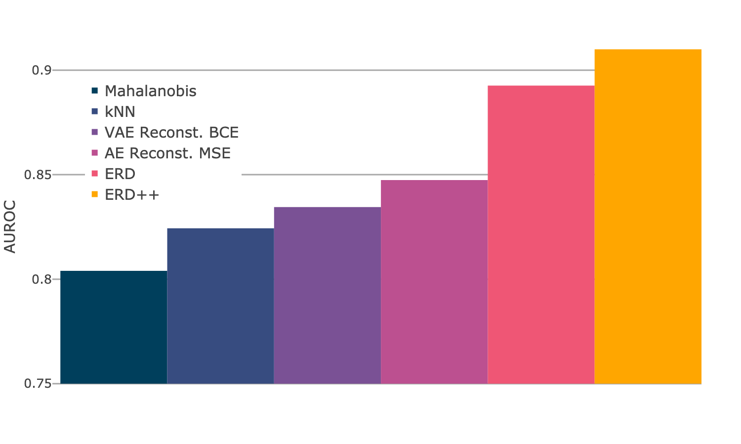
For the medical novelty detection benchmark we show in Figure 5(a) the average AUROC achieved by some representative baselines taken from Cao2020 [6]. Our method improves the average AUROC from $0.85$ to $0.91$, compared to the best baseline. We refer the reader to Cao2020 [6] for precise details on the methods. Appendix G contains more results, as well as additional baselines.

(a) Novelty detection performance on medical data

(b) Effect of OOD proportion on detection

Figure 5: Left: AUROC averaged over all scenarios in the medical novelty detection benchmark. The values for the baselines are computed using the code from Cao2020 [6]. Right: The AUROC of a 3-model ERD ensemble as the number and proportion of ID (CIFAR10[0:4]) and OOD (CIFAR10[5:9]) samples in the unlabeled set are varied (see also Appendix I).

4.5 Ablation studies and limitations

We also perform extensive experiments to understand the importance of specific design choices and hyperparameters, and refer the reader to the appendix for details.

Relaxing assumptions on OOD samples.

In Table 1 we evaluate our approach on a holdout test set that is drawn from the same distribution as the unlabeled set $U$ used for fine-tuning. However, we provide experiments in Appendix F.10 that show that novelty detection with ERD continues to perform well even when the test set and $U$ come from different distributions (e.g. novel-class data in the test set also suffers from corruptions). Further, even though our main focus is novel-class detection, our experiments (Appendix F.4) indicate that ERD can also successfully identify near OOD samples that suffer from only mild covariate shift compared to the ID data (e.g. CIFAR10 vs corrupted CIFAR10 [18] or CIFAR10v2 [39]). Finally, Appendix F.1 shows that ERD ensembles also perform well in a transductive setting [44], where the test set coincides with $U$.

Relaxing the assumptions of Proposition 3.1.

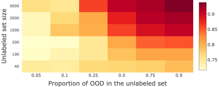
Our theoretical results require that the ID classes in the training set and the novel classes in $U$ have similar cardinality. In fact, this condition is unnecessarily strong as we show in our empirical analysis: In all experimental settings we have significantly fewer OOD than ID training points. We further investigate the impact of the size of the unlabeled set and of the ratio of novel samples in it ($\frac{|U_{\mathrm{OOD}}|}{|U_{\mathrm{ID}}|+|U_{\mathrm{OOD}}|}$) and find that ERD in fact maintains good performance for a broad range of ratios in Figure 5(b).

Sensitivity to hyperparameter choices.

We point out that ERD ensembles are particularly robust to changes in the hyperparameters like batch size or learning rate (Appendix H), or the choice of the arbitrary label assigned to the unlabeled set (Appendix F.9). Further, we note that ERD ensembles with as few as two models already show remarkable novelty detection performance and refer to Appendix F.9 for experiments with larger ensemble sizes. Moreover, ERD performance improves with larger neural networks (Appendix F.8), meaning that ERD will benefit from any future advances in architecture design.

Choice of disagreement score.

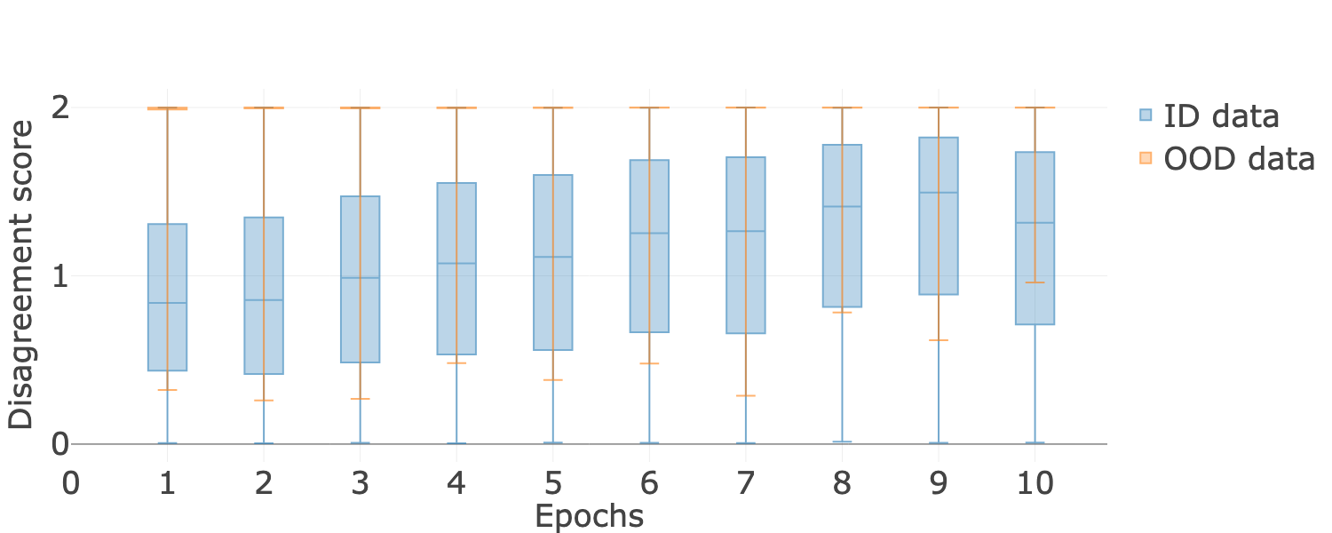
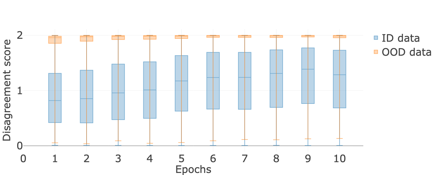
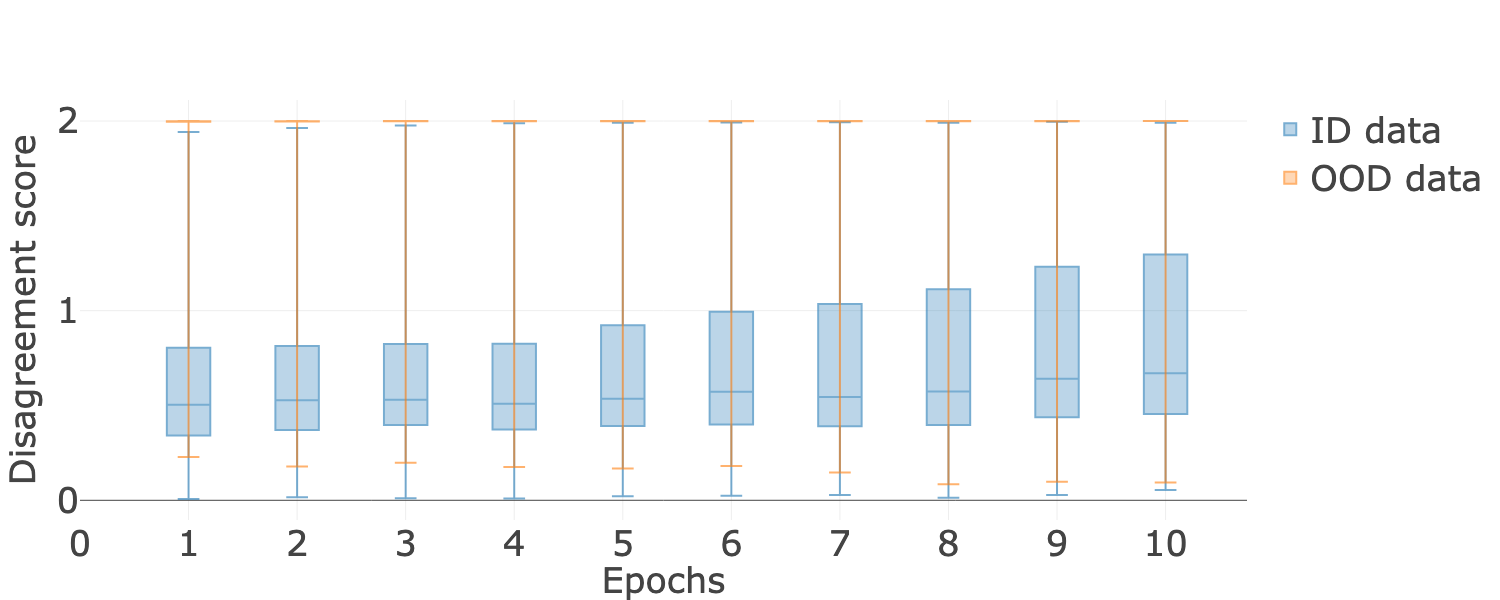
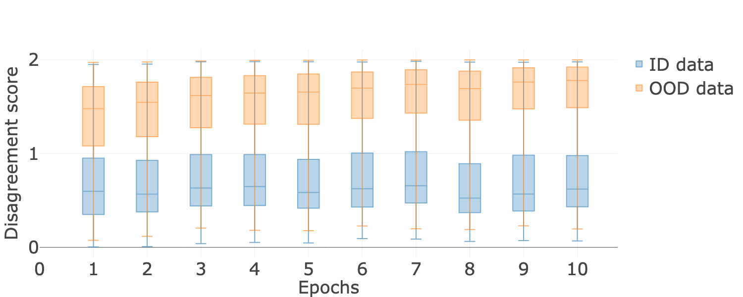
We show in Table 3 in Appendix B, that the training procedure alone (Algorithm 1) does not suffice for good novelty detection. For optimal results, ERD ensembles need to be combined with a disagreement-based score like the one introduced in Section 2.3. Finally, we show how the distribution of the disagreement score changes during training for ERD (Appendix K) and explain why regularizing disagreement is more challenging for near OOD data, compared to easier, far OOD settings (Appendix J).

Limitations.

Despite the advantages of ERD, like all prior SSND methods, our approach is not a good fit for online (real-time) novelty detection tasks. Moreover, ERD ensembles are not tailored to anomaly detection, where outliers are particularly rare, since the unlabeled set should contain at least a small number of samples from the novel classes (see Figure 5(b) and Appendix I). However, ERD ensembles are an ideal candidate for applications that require highly accurate, offline novelty detection, like the one illustrated in Figure 1.

5 Related work

Table 2: Taxonomy of novelty detection methods, categorized according to data availability (horizontal axis) and probabilistic perspective (vertical axis). We highlight the ensemble-based methods.

	UND	SSND	Different OOD A-UND	Synthetic OOD A-UND	P-UND	SND
Learn $P_{X}$	Generative e.g. [AAB18], OC classif. e.g. [SPSSW01]	nnPU [KNPS17]		OC classif. [SLYJP21, TMJS20]	[RH21]	[GKRB13, DKT19, RVGBM20]
Learn $P_{X}$ using $y$	Gram [SO19], OpenHybrid [ZLGG20]	ERD (Ours), SSND for shallow models [MBGBM10, BLS10], U-LAC [DYZ14, ZZMZ20]		Data augmentation for contrastive loss [TMJS20, LA20]	ViT [FRL20]	Mahala. [LLLS18], MCD [YA19]
Uncertainty of $P_{Y|X}$	Bayesian methods e.g. [GG16], Vanilla Ensemble [LPB17]	—	DPN [MG18], OE [HMD19]	GAN outputs [LLLS18], noise [HTLI19] or uniform samples ([JLMG20])		ODIN [LLS18]

In this section, we present an overview of different types of related methods that are in principle applicable for solving semi-supervised novelty detection. In particular, we indicate caveats of these methods based on their categorization with respect to 1) data availability and 2) the surrogate objective they try to optimize. This taxonomy may also be of independent interest to navigate the zoo of ND methods. We list a few representative approaches in Table 2 and refer the reader to surveys such as Bulusu2020 [4] for a thorough literature overview.

5.1 Taxonomy according to data availability

In this section we present related novelty detection methods that use varying degrees of labeled OOD data for training. We call test OOD the novel-class data that we want to detect at test time.

In a scenario like the one in Figure 1, one can apply unsupervised novelty detection (UND) methods that ignore the unlabeled batch and only uses ID data during training [26, 43, 36]. However, these approaches lead to poor novelty detection performance, especially on near OOD data.

There are methods that suggest to improve UND performance by using additional data. For example, during training one may use synthetically generated outliers (e.g. Tack2020 [50, 47]) or a different OOD data set that may be available (e.g. OE and DPN use TinyImages) with samples known to be outliers. However, in order for these augmented unsupervised ND (A-UND) methods to work, they require that the OOD data used for training is similar to test OOD samples. When this condition is not satisfied, A-UND performance deteriorates drastically (see Table 1). However, by definition, novel data is unknown and the only information about the OOD data that is realistically available is in the unlabeled set like in SSND. Therefore, it is unknown what an appropriate choice of the training OOD data is for A-UND methods.

Another line of work uses pretrained models to incorporate additional data that is close to test OOD samples, i.e. pretrained UND (P-UND). fort2021 [11] use large transformer models pretrained on ImageNet21k and achieve good near OOD detection performance when ID and OOD data are similar to ImageNet samples (e.g. CIFAR10/CIFAR100). However, our experiments in Appendix F.3 reveal that this method performs poorly on all other near OOD data sets, including unseen FashionMNIST or SVHN classes and X-rays of unknown diseases. This unsatisfactory performance is apparent when ID and OOD data do not share visual features with the pretraining data (i.e. ImageNet21k). Since collecting such large troves of “similar” data for pre-training is often not possible in practical applications (as medical imaging), the use case of their method is rather limited.

Furthermore, a few popular methods use test OOD data for calibration or hyperparameter tuning [54, 28, 30, 42], which is not applicable in practice. Clearly, knowing the test OOD distribution a priori turns the problem into supervised ND (SND), and hence, violates the fundamental assumption that OOD data is unforeseeable.

As we have already seen, current SSND approaches (e.g. MCD, nnPU) perform poorly for complex models such as neural networks. We note that SSND is similar to using unlabeled data for learning with augmented classes (U-LAC) [7, 15, 57] and is related to transductive novelty detection [44, 15], where the test set coincides with the unlabeled set used for training.

5.2 Taxonomy according to probabilistic perspective

Apart from data availability, the methods that we can use in a practical SSND scenario implicitly or explicitly use a different principle based on a probabilistic model. For example, novel-class samples are a subset of the points that are out-of-distribution in the literal sense, i.e. $P_{X}(x)<\alpha$. One can hence learn $P_{X}$ from unlabeled ID data, which is however notoriously difficult in high dimensions.

Similarly, from a Bayesian viewpoint, the predictive variance is larger for OOD samples with $P_{X}(x)<\alpha$. Hence, one could instead compute the posterior $P_{X}(y|x)$ and flag points with large variance (i.e. high predictive uncertainty). This circumvents the problem with estimating $P_{X}$. However, Bayesian estimates of uncertainty that accompany NN predictions tend to not be accurate on OOD data [38], resulting in poor novelty detection performance.

When the labels are available for the training set, we can instead partially learn $P_{X}$ using $y$. For instance, one could use generative modeling to estimate the set of $x$ for which $P_{X}(x)>\alpha$ via $P_{X}(x|y)$ [28, 43]. Alternatively, given a loss and function space, we may use the labels indirectly, like in ERD, and use properties of the approximated population error that imply small or large $P_{X}$.

6 Conclusion

In summary, we propose an SSND procedure that exploits unlabeled data effectively to generate an ensemble with regularized disagreement, which achieves remarkable novelty detection performance. Our SSND method does not need labeled OOD data during training unlike many other related works summarized in Table 2.

We leave as future work a thorough investigation of the impact of the labeling scheme of the unlabeled set on the sample complexity of the method, as well as an analysis of the trade-off governed by the complexity of the model class.

Acknowledgments

We are grateful to Călin Cruceru, Gideon Dresdner, Alexander Immer, Sidak Pal Singh and Armeen Taeb for feedback on the manuscript and to Ayush Garg for preliminary experiments. We also thank the anonymous reviewers for their helpful remarks.

Appendix A Theoretical statements

Definition A.1 ($({\epsilon},\rho)$-clusterable data set).

We say that a data set $\mathcal{D}=\{(x_{i},y_{i})\}_{i=1}^{n}$ is (${\epsilon},\rho$)-clusterable for fixed ${\epsilon}>0$ and $\rho\in[0,1]$ if there exists a partitioning of it into subsets $\{C_{1},...,C_{K}\},$ which we call clusters, each with their associated unit-norm cluster center $c_{i}$, that satisfy the following conditions:

• $\bigcup_{i=1}^{K}C_{i}=\mathcal{D}$ and $C_{i}\cap C_{j}=\emptyset,\forall i,j\in[K]$;

• all the points in a cluster lie in the ${\epsilon}$-neighborhood of their corresponding cluster center, i.e. $||x-c_{i}||_{2}\leq{\epsilon}$ for all $x\in C_{i}$ and all $i\in[K]$;

• a fraction of at least $1-\rho$ of the points in each cluster $C_{i}$ have the same label, which we call the cluster label and denote $y^{*}(c_{i})$. The remaining points suffer from label noise;

• if two cluster $C_{i}$ and $C_{j}$ have different labels, then their centers are $2{\epsilon}$ far from each other, i.e. $||c_{i}-c_{j}||_{2}\geq 2{\epsilon}$;

• the clusters are balanced i.e. for all $i\in[K],\alpha_{1}\frac{n}{K}\leq|C_{i}|\leq\alpha_{2}\frac{n}{K}$, where $\alpha_{1}$ and $\alpha_{2}$ are two positive constants.

In our case, for a fixed label $c\in\mathcal{Y}$, we assume that the set $S\cup(U,c)$ is $({\epsilon},\rho)$-clusterable into $K$ clusters. We further assume that each cluster $C_{i}$ only includes a few noisy samples from $(U_{\mathrm{ID}}^{\neg c},c)$, i.e. $\frac{|C_{i}\cap(U_{\mathrm{ID}}^{\neg c},c)|}{|C_{i}|}\leq\rho$ and that for clusters $C_{i}$ whose cluster label is not $c$, i.e. $y^{*}(c_{i})\neq c$, it holds that $C_{i}\cap(U_{\mathrm{OOD}},c)=\emptyset$.

We define the matrices $C:=[c_{1},...,c_{K}]^{T}\in\mathbb{R}^{K\times d}$ and $\Sigma:=(CC^{T})\bigodot\mathbb{E}_{g}[\phi^{\prime}(Cg)\phi^{\prime}(Cg)^{T}]$, with $g\sim\mathcal{N}(0,I_{d})$ and where $\bigodot$ denotes the elementwise product. We use $\|\cdot\|$ and $\lambda_{min}(\cdot)$ to denote the spectral norm and the smallest eigenvalue of a matrix, respectively.

For prediction, we consider a 2-layer neural network model with $p$ hidden units, where $p\gtrsim\frac{K^{2}\|C\|^{4}}{\lambda_{min}(\Sigma)^{4}}$. We can write this model as follows:

$$x\mapsto f(x;W)=v^{T}\phi(Wx),$$ (1)

The first layer weights $W$ are initialized with random values drawn from $\mathcal{N}(0,1)$, while the last layer weights $v$ have fixed values: half of them are set to $1/p$ and the other half is $-1/p$. We consider activation functions $\phi$ with bounded first and second order derivatives, i.e. $|\phi^{\prime}(x)|\leq\Gamma$ and $\phi^{\prime\prime}(x)\leq\Gamma$. We use the squared loss for training, i.e. $\mathcal{L}(W)=\frac{1}{2}\sum_{i=0}^{n}(y_{i}-f(x_{i};W))^{2}$ and take gradient descent steps to find the optimum of the loss function, i.e. $W_{\tau+1}=W_{\tau}-\eta\nabla\mathcal{L}(W_{\tau})$, where the step size is set to $\eta\simeq\frac{K}{n\|C\|^{2}}$.

We can now state the following proposition:

Proposition A.1.

Assume that $\rho\leq\delta/8$ and ${\epsilon}\leq\alpha\delta\lambda_{min}(\Sigma)^{2}/K^{2}$, where $\delta$ is a constant such that $\delta\leq\frac{2}{|\mathcal{Y}-1|}$ and $\alpha$ is a constant that depends on $\Gamma$. Then it holds with high probability $1-3/K^{100}-Ke^{-100d}$ over the initialization of the weights that the neural network trained on $S\cup(U,c)$ perfectly fits $S$, $(U_{\mathrm{ID}}^{c},c)$ and $(U_{\mathrm{OOD}},c)$, but not $(U_{\mathrm{ID}}^{\neg c},c)$, after $T=c_{4}\frac{\|C\|^{2}}{\lambda_{min}(\Sigma)}$ iterations.

This result shows that there exists an optimal stopping time at which the neural network predicts the correct label on all ID points and the label $c$ on all the OOD points. As we will see later in the proof, the proposition is derived from a more general result which shows that the early stopped model predicts these labels not only on the points in $U$ but also in an ${\epsilon}$-neighborhood around cluster centers. Hence, an ERD ensemble can be used to detect holdout OOD samples similar to the ones in $U$, after being tuned on $U$. This follows the intuition that classifiers regularized with early stopping are smooth and generalize well.

The clusterable data model is generic enough to include data sets with non-linear decision boundaries. Moreover, notice that the condition in Proposition A.1 is satisfied when $S\cup(U_{\mathrm{ID}},c)$ is $({\epsilon},\rho)$-clusterable and $(U_{\mathrm{OOD}},c)$ is ${\epsilon}$-clusterable and if the cluster centers of $(U_{\mathrm{OOD}},c)$ are at distance at least $2{\epsilon}$ from the cluster centers of $S\cup(U_{\mathrm{ID}},c)$. A situation in which these requirements are met is, for instance, when the OOD data comes from novel classes, when all classes (including the unseen ones that are not in the training set) are well separated, with cluster centers at least $2{\epsilon}$ away in Euclidean distance. In addition, in order to limit the amount of label noise in each cluster, it is necessary that the number of incorrectly labeled samples in $(U_{\mathrm{ID}}^{\neg c},c)$ is small, relative to the size of $S$.

In practice, we only need that the decision boundary separating $(U_{\mathrm{OOD}},c)$ from $S$ is easier to learn than the classifier required to interpolate the incorrectly labeled $(U_{\mathrm{ID}}^{\neg c},c)$, which is often the case, provided that $(U_{\mathrm{OOD}},c)$ is large enough and the OOD samples come from novel classes.

We now provide the proof for Proposition A.1:

Proof.

We begin by restating a result from mahdi [29]:

Theorem A.1 ([29]).

Let $\mathcal{D}:=\{(x_{i},y_{i})\}\in\mathbb{R}^{d}\times\mathcal{Y}$ be an $({\epsilon},\rho)$-clusterable training set, with ${\epsilon}\leq c_{1}\delta\lambda_{min}(\Sigma)^{2}/K^{2}$ and $\rho\leq\delta/8$, where $\delta$ is a constant that satisfies $\delta\leq\frac{2}{|\mathcal{Y}|-1}$. Consider a two-layer neural network as described above, and train it with gradient descent starting from initial weights sampled i.i.d. from $\mathcal{N}(0,1)$. Assume further that the step size is $\eta=c_{2}\frac{K}{n\|C\|^{2}}$ and that the number of hidden units $p$ is at least $c_{3}\frac{K^{2}\|C\|^{4}}{\lambda_{min}(\Sigma)^{4}}$. Under these conditions, it holds with probability at least $1-3/K^{100}-Ke^{-100d}$ over the random draws of the initial weights, that after $T=c_{4}\frac{\|C\|^{2}}{\lambda_{min}(\Sigma)}$ gradient descent steps, the neural network $x\mapsto f(x;W_{T})$ predicts the correct cluster label for all points in the ${\epsilon}$-neighborhood of the cluster center, namely:

$$\arg\max_{y\in\mathcal{Y}}|f(x;W_{T})-\omega(y)|=y^{*}(c_{i}),\text{ for all }x\text{ with }\|x-c_{i}\|_{2}\leq{\epsilon}\text{ and all clusters }i\in[K],$$ (2)

where $\omega:\mathcal{Y}\to\{0,1\}^{|\mathcal{Y}|}$ yields one-hot embeddings of the labels. The constants $c_{1},c_{2},c_{3},c_{4}$ depend only on $\Gamma$.

Notice that, under the assumptions introduced above, the set $S\cup(U,c)$ is $({\epsilon},\rho)$-clusterable, since the incorrectly labeled ID points in $(U_{\mathrm{ID}}^{\neg c},c)$ constitute at most a fraction $\rho$ of the clusters they belong to. As a consequence, Proposition A.1 follows directly from Theorem A.1.

∎

Appendix B Disagreement score for novelty detection

Figure 6: Cartoon illustration showing a diverse ensemble of linear binary classifiers. We compare novelty detection performance for two aggregation scores: $(\text{H}\circ\text{Avg})$ (Left) and $(\text{Avg}\circ\rho)$ with $\rho(f_{1}(x),f_{2}(x))=\mathbb{1}_{\operatorname{sgn}(f_{1}(x))\neq\operatorname{sgn}(f_{2}(x))}$ (Right). The two metrics achieve similar TPRs, but using $(\text{H}\circ\text{Avg})$ instead of our score, $(\text{Avg}\circ\rho)$, leads to more false positives, since the former simply flags as OOD a band around the averaged model (solid black line) and does not take advantage of the ensemble’s diversity.

As we argue in Section 3, Algorithm 1 produces an ensemble that disagrees on OOD data, and hence, we want to devise a scalar score that reflects this model diversity. Previous works [26, 38] first average the softmax predictions of the models in the ensemble and then use the entropy as a metric, i.e. $(\text{H}\circ\text{Avg})(f_{1}(x),...,f_{K}(x)):=-\sum_{i=1}^{|\mathcal{Y}|}(f(x))_{i}\log(f(x))_{i}$ where $f(x):=\frac{1}{K}\sum_{i=1}^{K}f_{i}(x)$ and $(f(x))_{i}$ is the $i^{\text{th}}$ element of $f(x)\in[0,1]^{|\mathcal{Y}|}$. We argue later that averaging discards information about the diversity of the models.

Recall that our average pairwise disagreement between the outputs of $K$ models in an ensemble reads:

$$(\text{Avg}\circ\rho)(f_{1}(x),...,f_{K}(x)):=\frac{2}{K(K-1)}\sum_{i\neq j}\rho\left(f_{i}(x),f_{j}(x)\right),$$ (3)

where $\rho$ is a measure of disagreement between the softmax outputs of two predictors, for example the total variation distance $\rho_{\text{TV}}(f_{i}(x),f_{j}(x))=\frac{1}{2}\|f_{i}(x)-f_{j}(x)\|_{1}$ used in our experiments.

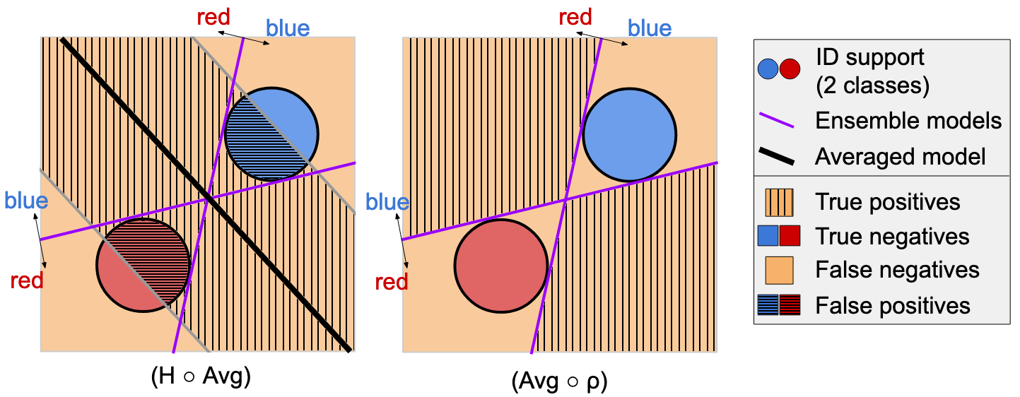
We briefly highlight the reason why averaging softmax outputs first like in previous works relinquishes all the benefits of having a more diverse ensemble, as opposed to the proposed pairwise score in Equation 3. Recall that varying thresholds yield different true negative and true positive rates (TNR and TPR, respectively) for a given statistic. In the sketch in Figure 6 we show that the score we propose, $(\text{Avg}\circ\rho)$, achieves a higher TNR compared to $(\text{H}\circ\text{Avg})$, for a fixed TPR, which is a common way of evaluating statistical tests. Notice that the detection region for $(\text{H}\circ\text{Avg})$ is always limited to a band around the average model for any threshold value $t_{0}$. In order for the $(\text{H}\circ\text{Avg})$ to have large TPR, this band needs to be wide, leading to many false positives. Instead, our disagreement score exploits the diversity of the models to more accurately detect OOD data.

Figure 7: Relying only on the randomness of SGD and of the weight initialization to diversify models is not enough, as it often yields similar classifiers. Each column shows a different predictor trained from random initializations with Adam. All models have the same 1-hidden layer MLP architecture.

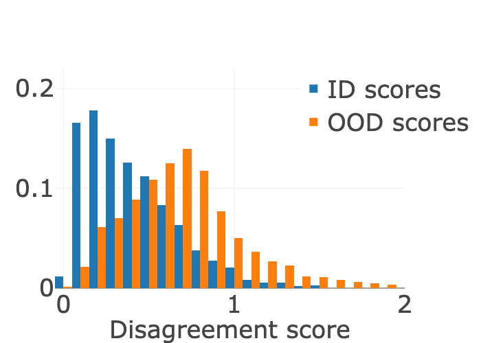
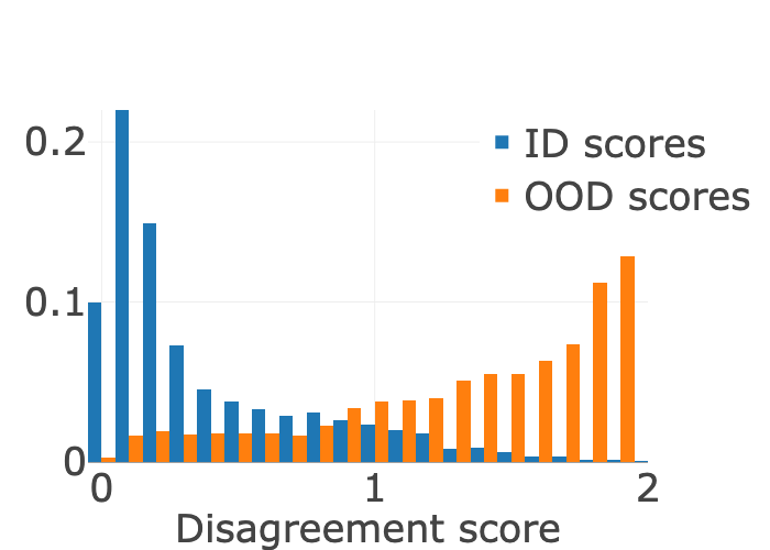
We now provide further quantitative evidence to support the intuition presented in Figure 6. The aggregation metric is tailored to exploit ensemble diversity, which makes it particularly beneficial for ERD. On the other hand, Vanilla Ensembles only rely on the stochasticity of the training process and the random initializations of the weights to produce diverse models, which often leads to classifiers that are strikingly similar as we show in Figure 7 for a few 2D data sets. As a consequence, using our disagreement score $(\text{Avg}\circ\rho)$ for Vanilla Ensembles can sometimes hurt novelty detection performance. To see this, consider the extreme situation in which the models in the ensemble are identical, i.e. $f_{1}=f_{2}$. Then it follows that $(\text{Avg}\circ\rho)(f_{1}(x),f_{2}(x))=0$, for all test points $x$ and for any function $\rho$ that satisfies the distance axioms.

We note that the disagreement score that we propose takes a form that is similar to previous diversity scores, e.g. Zhang2010 [56, 54]. In the context of regression, one can measure uncertainty using the variance of the outputs metric previously employed in works such as gal2016 [12]. However, we point out that using the output variance requires that the ensemble is the result of sampling from a random process (e.g. sampling different training data for the models, or sampling different parameters from a posterior). In our framework, we obtain the ensemble by solving a different optimization problem for each of the models by assigning a different label to the unlabeled data. Therefore, despite their similarities, our disagreement score and the output variance are, on a conceptual level, fundamentally different metrics.

Table 3 shows that $(\text{Avg}\circ\rho)$ leads to worse novelty detection performance for Vanilla Ensembles, compared to using the entropy of the average softmax score, $(\text{H}\circ\text{Avg})$, which was proposed in prior work. However, if the ensembles are indeed diverse, as we argue is the case for our method ERD (see Section 3), then there is a clear advantage to using a score that, unlike $(\text{H}\circ\text{Avg})$, takes diversity into account, as shown in Table 3 for 5-model ERD ensembles.

Table 3: The disagreement score that we propose $(\text{Avg}\circ\rho)$ exploits ensemble diversity and benefits in particular ERD ensembles. Novelty detection performance is significantly improved when using $(\text{Avg}\circ\rho)$ compared to the previously proposed $(\text{H}\circ\text{Avg})$ metric. Since Vanilla Ensemble are not diverse enough, a score that relies on model diversity can hurt novelty detection performance. We highlight the AUROC and the TNR@95 obtained with the score function that is best for Vanilla Ensemble and the best for ERD.

ID data	OOD data	Vanilla Ensembles $(\text{H}\circ\text{Avg})$	Vanilla Ensembles $(\text{Avg}\circ\rho)$	ERD $(\text{H}\circ\text{Avg})$	ERD $(\text{Avg}\circ\rho)$
		AUROC $\uparrow$ / TNR@95 $\uparrow$
SVHN	CIFAR10	0.97 / 0.88	0.96 / 0.89	0.86 / 0.85	0.99 / 0.97
CIFAR10	SVHN	0.92 / 0.78	0.91 / 0.78	0.92 / 0.92	1.00 / 1.00
CIFAR100	SVHN	0.84 / 0.48	0.79 / 0.46	0.36 / 0.35	1.00 / 1.00
SVHN[0:4]	SVHN[5:9]	0.92 / 0.69	0.91 / 0.69	0.94 / 0.66	0.94 / 0.66
CIFAR10[0:4]	CIFAR10[5:9]	0.80 / 0.39	0.80 / 0.39	0.91 / 0.65	0.91 / 0.66
CIFAR100[0:49]	CIFAR100[50:99]	0.78 / 0.35	0.76 / 0.34	0.63 / 0.38	0.81 / 0.40
Average		0.87 / 0.60	0.86 / 0.59	0.77 / 0.64	0.94 / 0.78

We highlight once again that other methods that attempt to obtain diverse ensembles, such as MCD, fail to train models with sufficient disagreement, even when they use oracle OOD for hyperparameter tuning (Figure 8(a)).

(a) Not enough diversity (MCD)

(b) Regularized diversity (ERD)

Figure 8: Distribution of disagreement scores on ID and OOD data for an ensemble that is not diverse enough (Left), and an ensemble with regularized disagreement (Right). Note that MCD is early-stopped using oracle OOD data. ID=CIFAR10[0:4], OOD=CIFAR10[5:9].

Appendix C Taxonomy of OOD detection methods according to overall objective

We now provide more details regarding the categorization of OOD detection approaches based on the different surrogate objectives that they use in order to detect OOD samples.

Learning the ID marginal $P_{X}$.

We loosely define OOD samples as all $x$ for which $P_{X}(x)<\alpha$, for a small constant $\alpha>0$. Therefore, if we had access to the marginal training distribution $P_{X}$, we would have perfect OOD detection. Realistically, however, $P_{X}$ is unknown, and we need to resort to estimating it. Explicit density estimation with generative models [1, 36] is inherently difficult in high dimensions. Alternatively, one-class classification [35, 42, 47] and PU learning approaches [10, 24] try to directly learn a discriminator between ID and OOD data in the presence of known (e.g. A-UND) or unknown (e.g. SSND) OOD data. However, these methods tend to produce indistinguishable representations for inliers and outliers when the ID distribution consists of many diverse classes.

Learning $P_{X}$ using label information (ours).

Since in a prediction problem, the ID training set has class labels, one can take advantage of that additional information to distinguish points in the support of $P_{X}$ from OOD data. For instance, mahalanobis [28, 43] propose to use the intermediate representations of neural networks trained for prediction to detect OOD data. Often, the task is to also simultaneously predict well on ID data, a problem known as open-set recognition [13] and tackled by approaches like OpenHybrid [55].

Learning uncertainty estimates for $P_{Y|X}$.

In the prediction setting, calibrated uncertainty estimates error could naturally be used to detect OOD samples. Many uncertainty quantification methods are based on a Bayesian framework [12, 34] or calibration improvement [30, 16]. However, neither of them perform as well as other OOD methods mentioned above [38].

Appendix D Experiment details

D.1 Baselines

In this section we describe in detail the baselines with which we compare our method and describe how we choose their hyperparameters. For all baselines we use the hyperparameters suggested by the authors for the respective data sets (e.g. different hyperparameters for CIFAR10 or ImageNet). For all methods, we use pretrained models provided by the authors. However, we note that for the novel-class settings, pretraining on the entire training set means that the model is exposed to the OOD classes as well, which is undesirable. Therefore, for these settings we pretrain only on the split of the training set that contains the ID classes. Since the classification problem is similar to the original one of training on the entire training set, we use the same hyperparameters that the authors report in the original papers.

Moreover, we point out that even though different methods use different model architectures, that is not inherently unreasonable when the goal is novelty detection, since it is not clear if a complex model is more desirable than a smaller model. For this reason, we use the model architecture recommended by the authors of the baselines and which was used to produce the good results reported in their published works. For Vanilla Ensembles and for ERD we show results for different architectures in Appendix F.8.

• Vanilla Ensembles [26]: We train an ensemble on the training set according to the true labels. For a test sample, we average the outputs of the softmax probabilities predicted by the models, and use the entropy of the resulting distribution as the score for the hypothesis test described in Section 2.3. We use ensembles of 5 models, with the same architecture and hyperparameters as the ones used for ERD. Hyperparameters are tuned to achieve good validation accuracy.

• Gram method [43]: The Gram baseline is similar to the Mahalanobis method in that both use the intermediate feature representations obtained with a deep neural network to determine whether a test point is an outlier. However, what sets the Gram method apart is the fact that it does not need any OOD data for training or calibration. We use the pretrained models provided by the authors, or train our own, using the same methodology as described for the Mahalanobis baseline. For OOD detection, we use the code published by the authors. We note that for MLP models, the Gram method is difficult to tune and we could not find a configuration that works well, despite our best efforts and following the suggestions proposed during our communication with the authors.

• Deep Prior Networks (DPN) [34]: DPN is a Bayesian Method that trains a neural network (Prior Network) to parametrize a Dirichlet distribution over the class probabilities. We train a WideResNet WRN-28-10 for $100$ epochs using SGD with momentum $0.9$, with an initial learning rate of $0.01$, which is decayed by $0.2$ at epochs $50$, $70$, and $90$. For MNIST, we use EMINST/Letters as OOD for tuning. For all other settings, we use TinyImages as OOD for tuning.

• Outlier Exposure [20]: This approach makes a model’s softmax predictions close to the uniform distribution on the known outliers, while maintaining a good classification performance on the training distribution. We use the WideResNet architecture (WRN). For fine-tuning, we use the settings recommended by the authors, namely we train for $10$ epochs with learning rate $0.001$. For training from scratch, we train for $100$ epochs with an initial learning rate of $0.1$. When the training data set is either CIFAR10/CIFAR100 or ImageNet, we use the default WRN parameters of the author’s code, namely $40$ layers, $2$ widen-factor, droprate $0.3$. When the training dataset is SVHN, we use the author’s recommended parameters of $16$ layers, $4$ widen-factor and droprate $0.4$. All settings use the cosine annealing learning rate scheduler provided with the author’s code, without any modifications. For all settings, we use TinyImages as known OOD data during training. In Section F.6 we show results for known OOD data that is similar to the OOD data used for testing.

• Mahalanobis [28]: The method pretrains models on the labeled training data. For a test data point, it uses the intermediate representations of each layer as “extracted features”. It then performs binary classification using logistic regression using these extracted features. In the original setting, the classification is done on “training” ID vs “training” OOD samples (which are from the same distribution as the test OOD samples). Furthermore, hyperparameter tuning for the optimal amount of noise is performed on validation ID and OOD data. We use the WRN-28-10 architecture, pretrained for $200$ epochs. The initial learning rate is $0.1$, which is decayed at epochs $60$, $120$, and $160$ by $0.2$. We use SGD with momentum $0.9$, and the standard weight decay of $5\cdot 10^{-4}$. The code published for the Mahalanobis method performs a hyperparameter search automatically for each of the data sets.

The following baselines attempt to leverage the unlabeled data that is available in applications such as the one depicted in Figure 1, similar to ERD.

• Non-negative PU learning (nnPU) [24]: The method trains a binary predictor to distinguish between a set of known positives (in our case the ID data) and a set that contains a mixture of positives and negatives (in our case the unlabeled set). To prevent the interpolation of all the unlabeled samples, Kiryo17 [24] proposes a regularized objective. It is important to note that most training objectives in the PU learning literature require that the ratio between the positives and negatives in the unlabeled set is known or easy to estimate. For our experiments we always use the exact OOD ratio to train the nnPU baseline. Therefore, we obtain an upper bound on the AUROC/TNR@95. If the ratio is estimated from finite samples, then estimation errors may lead to slightly worse OOD detection performance. We perform a grid search over the learning rate and the threshold that appears in the nnPU regularizer and pick the option with the best validation accuracy measured on a holdout set with only positive samples (in our case, ID data).

• Maximum Classifier Discrepancy (MCD) [54]: The MCD method trains two classifiers at the same time, and makes them disagree on the unlabeled data, while maintaining good classification performance. We use the WRN-28-10 architecture as suggested in the paper. We did not change the default parameters which came with the author’s code, so weight decay is $10^{-4}$, and the optimizer is SGD with momentum $0.9$. When available (for CIFAR10 and CIFAR100), we use the pretrained models provided by the authors. For the other training datasets, we use their methodology to generate pretrained models: We train a WRN-28-10 for 200 epochs. The learning rate starts at 0.1 and drops by a factor of 10 at $50\%$ and $75\%$ of the training progress.

• Mahalanobis-U: This is a slightly different version of the Mahalanobis baseline, for which we use early-stopped logistic regression to distinguish between the training set and an unlabeled set with ID and OOD samples (instead of discriminating a known OOD set from the inliers). The early stopping iteration is chosen to minimize the classification errors on a validation set that contains only ID data (recall that we do not assume to know which are the OOD samples).

In addition to these approaches that have been introduced in prior work, we also propose a strong novel baseline that that bares some similarity to PU learning and to ERD.

• Binary classifier The approach consists in discriminating between the labeled ID training set and the mixed unlabeled set, that contains both ID and OOD data. We use regularization to prevent the trivial solution for which the entire unlabeled set is predicted as OOD. Unlike PU learning, the binary classifier does not require that the OOD ratio in the test distribution is known. The approach is similar to a method described in [44] which also requires that the OOD ratio of the unlabeled set is known. We tune the learning rate and the weight of the unlabeled samples in the training loss by performing a grid search and selecting the configuration with the best validation accuracy, computed on a holdout set containing only ID samples. We note that the binary classifier that appears in Section G in the medical benchmark, is not the same as this baseline. For more details on the binary classifier that appears in the medical data experiments we refer the reader to Cao2020 [6].

D.2 Training configuration for ERD

For ERD we always use hyperparameters that give the best validation accuracy when training a model on the ID training set. In other words, we pick hyperparameter values that lead to good ID generalization and do not perform further hyperparameter tuning for the different OOD data sets on which we evaluate our approach. We point out that, if the ID labeled set is known to suffer from class imbalance, subpopulation imbalance or label noise, any training method that addresses these issues can be used instead of standard empirical risk minimization to train our ensemble (e.g. see mahdi [29]).

For MNIST and FashionMNIST, we train ensembles of 3-layer MLP models with ReLU activations. Each intermediate layer has 100 neurons. The models are optimized using Adam, with a learning rate of $0.001$, for $10$ epochs.

For SVHN, CIFAR10/CIFAR100 and ImageNet, we train ensembles of ResNet20 [17]. The models are initialized with weights pretrained for $100$ epochs on the labeled training set. We fine-tune each model for 10 epochs using SGD with momentum $0.9$, and a learning rate of $0.001$. The weights are trained with an $\ell_{2}$ regularization coefficient of $5e-4$. We use a batch size of 128 for all scenarios, unless explicitly stated otherwise. We used the same hyperparameters for all settings.

For pretraining, we perform SGD for 100 epochs and use the same architecture and hyperparameters as described above, with the exception of the learning rate that starts at $0.1$, and is multiplied by $0.2$ at epochs $50$, $70$ and $90$.

Apart from ERD, which fine-tunes the ensemble models starting from pretrained weights, we also present in the Appendix results for ERD++. This variant of our method trains the models from random initializations, and hence needs more iterations to converge, making it more computationally expensive than ERD. We train all models in the ERD++ ensembles for $100$ epochs with a learning rate that starts at $0.1$, and is multiplied by $0.2$ at epochs $50$, $70$ and $90$. All other hyperparameters are the same as for ERD ensembles.

For the medical data sets, we train a Densenet-121 as the authors do in the original paper [6]. For ERD++, we do not use random weight initializations, but instead we start with the ImageNet weights provided with Tensorflow. The training configuration is exactly the same as for ResNet20, except that we use a batch size of 32 due to GPU memory restrictions, and for fine tuning we use a constant learning rate of $10^{-5}$.

D.3 Computational considerations for ERD

We note that ERD models reach the optimal stopping time within the first 10 epochs on all the data sets that we consider, which amounts to around $6$ minutes of training time if the models in the ensemble are fine-tuned in parallel on NVIDIA 1080 Ti GPUs. This is substantially better than the cost of fine-tuning a large ViT transformer model (which takes about 1 hour for 2500 iterations on the same hardware). Moreover, since the loss we use to train the ensemble decouples over the models, it allows for easy parallelization, unlike objectives like MCD where the ensemble models are intertwined.

Appendix E ID and OOD data sets

E.1 Data sets

For evaluation, we use the following image data sets: MNIST [27], Fashion MNIST [52], SVHN [37], CIFAR10 and CIFAR100 [25].

For the experiments using MNIST and FashionMNIST the training set size is 50K, the validation size is 10K, and the test ID and test OOD sizes are both 10K. For SVHN, CIFAR10 and CIFAR100, the training set size is 40K, the validation size is 10K, and the unlabeled set contains 10K samples: 5K are ID and 5K are OOD. For evaluation, we use a holdout set of 10K examples (half ID, half OOD). For the settings that use half of the classes as ID and the other half as OOD, all the sizes are divided by 2.

E.2 Samples for the settings with novel classes

(a)

(b)

Figure 9: (a) Data samples for the MNIST/FashionMNIST splits. (b) Data samples for the CIFAR10/SVHN splits.

Appendix F More experiments

We now present more experimental results that provide additional insights about the proposed approach. We note that, unless otherwise specified, we use 5-model ERD ensembles in this section.

F.1 Evaluation on the unlabeled set

In the main text we describe how one can leverage the unlabeled set $U$ to obtain an novelty detection algorithm that accurately identifies outliers at test time that similar to the ones in $U$. It is, however, possible to also use our method ERD to flag the OOD samples contained in the same set $U$ used for fine-tuning the ensemble. In Table 4 we show that the novelty detection performance of ERD is similar regardless of whether we use $U$ for evaluation, or a holdout test set $T$ drawn from the same distribution as $U$.

Table 4: Comparison between the novelty detection performance of ERD when using a holdout test set $T$ for evaluation, or the same unlabeled set $U$ that was used for fine-tuning the models.

ID data	OOD data	ERD (eval on $T$)	ERD (eval on $U$)
		AUROC $\uparrow$ / TNR@95 $\uparrow$
SVHN	CIFAR10	1.00 / 0.99	1.00 / 0.99
CIFAR10	SVHN	1.00 / 1.00	1.00 / 1.00
CIFAR100	SVHN	1.00 / 1.00	1.00 / 1.00
FMNIST[0,2,3,7,8]	FMNIST[1,4,5,6,9]	0.94 / 0.67	0.94 / 0.67
SVHN[0:4]	SVHN[5:9]	0.95 / 0.74	0.96 / 0.79
CIFAR10[0:4]	CIFAR10[5:9]	0.93 / 0.70	0.93 / 0.69
CIFAR100[0:49]	CIFAR100[50:99]	0.82 / 0.44	0.80 / 0.36
Average		0.95 / 0.79	0.95 / 0.79

F.2 Comparison with other related works

We compare 5-model ERD ensembles to more OOD detection approaches. For various reasons we did not run these methods ourselves on the data sets for which we evaluate our method in Section 4 (e.g. code not available, unable to replicate published results, poor performance reported by the authors etc). We collected the AUROC numbers presented in Table 5 from the papers that introduce each method. We note that our approach shows an excellent overall performance, being consistently better than or on par with the related works that we consider. While the method of fort2021 [11] performs significantly better than all other baselines on CIFAR10/CIFAR100 tasks, we argue in Appendix F.3 that this is primarily due to the convenient choice of the data set used for pretraining the transformer models (i.e. Imagenet21k) which is strikingly similar to the ID and OOD data.

OpenHybrid [55] is an open set recognition approach which reports great near OOD detection performance. We note that, despite our best efforts, we did not manage to match in our own experiments the results reported in the paper, even after communicating with the authors and using the code that they have provided. Moreover, we point out that the performance of OpenHybrid seems to deteriorate significantly when the ID data consists of numerous classes, as is the case for CIFAR100.

Furthermore, we note that generative models [36, 1] and one-class classification approaches [42, 50, 47] showed generally bad performance, in particular on near OOD data. When the ID training set is made up of several diverse classes, it is difficult to represent accurately all the ID data, and only the ID data.

Table 5: AUROC numbers collected from the literature for a number of relevant OOD detection methods. We note that the method of fort2021 [11] (^†) uses a large scale visual transformer models pretrained on a superset of the OOD data, i.e. ImageNet21k, while the method of sehwag2021 [46] (^∗) uses oracle OOD samples for training from the same data set as test OOD. For the settings with random classes, the numbers are averages over 5 draws and the standard deviation is always strictly smaller than $0.01$ for our method.

ID data	OOD data	fort2021 [11]†	openhybrid2020 [55]	winkens2020 [51]	Tack2020 [50]	sehwag2021 [46]∗	liu2020hybrid [31]	yujie2020 [57]	ERD (ours)	ERD++ (ours)
CIFAR10	CIFAR100	98.52	0.95	0.92	0.92	0.93	0.91	-	0.92	0.95
CIFAR100	CIFAR10	96.23	0.85	0.78	-	0.78	-	-	0.91	0.94
SVHN: 6 random classes	SVHN: 4 random classes	-	0.94	-	-	-	-	0.91	0.94	0.94
CIFAR10: 6 random classes	CIFAR10: 4 random classes	-	0.94	-	-	-	-	0.85	0.94	0.97

F.3 Shortcomings of pretrained ViT models for novelty detection

In this section we provide further experimental results pointing to the fact that large pretrained transformer models [11] can only detect near OOD samples from certain specific data sets, and do not generalize well more broadly.

Implementation details.

We fine-tune visual transformer (ViT) models pretrained on Imagenet21k according the methodology described in fort2021 [11]. We report results using the ViT-S-16 architecture ( 22 million trainable parameters) which we fine-tune for 2500 iterations on labeled ID data. We use the hyperparameters suggested by the authors and always ensure that the prediction accuracy of the fine-tuned model on ID data is in the expected range. The code published by the authors uses three different test statistics to detect OOD data: the maximum softmax probability [19], the vanilla Mahalanobis distance [28] and a recently proposed variant of the Mahalanobis approach [40]. In Table 6 we present only the metrics obtained with the best-performing test statistic for ViT. We stress that this favors the ViT method significantly, as different test statistics seem to perform better on different data sets. Since test OOD data is unknown, it is not possible to select which test statistic to use a priori, and hence, we use oracle knowledge to give ViT models an unfair advantage.

Experimental results.

In Table 6 we compare pretrained visual transformers with 5-model ERD and ERD++ ensembles. Notably, the data sets can be partitioned in two clusters, based on ViT novelty detection performance. On the one hand, if the ID or OOD data comes from CIFAR10 or CIFAR100, ViT models can detect novel-class samples well. Perhaps surprisingly, ViT fails short of detecting OOD data perfectly (i.e. AUROC and TNR@95 of 1) on easy tasks such as CIFAR10 vs SVHN or CIFAR100 vs SVHN, unlike ERD and a number of other baseline approaches.

On the other hand, ViT shows remarkably poor performance on all other data sets, when neither the ID nor the OOD data come from CIFAR10/CIFAR100. This includes some of the novel disease use cases from the medical OOD detection benchmark (see Appendix G for more details about the data sets). This unsatisfactory performance persists even for larger ViT models (we have tried ViT-S-16 and ViT-B-16 architectures), when fine-tuning for more iterations (we have tried both 2500 and 10000 iterations), or when varying hyperparameters such as the learning rate.

Intuition for why ViT fails.

We conjecture that the novelty detection performance with pretrained ViT models relies heavily on the choice of the pretraining data set. In particular, we hypothesize that, since CIFAR10/CIFAR100 classes are included in the Imagenet21k data set used for pretraining, the models learn features that are useful for distinguishing ID and OOD classes when the ID and/or OOD data comes from CIFAR10/CIFAR100. Hence, this would explain the good performance of pretrained models on the data sets at the top of Table 6. On the other hand, when ID and OOD data is strikingly different from the pretraining data, both ID and OOD samples are projected to the same concentrated region of the representation space, which makes it difficult to detect novel-class points. Moreover, the process of fine-tuning as it is described in fort2021 [11] seems to not help to alleviate this problem. This leads to the poor performance observed on the near OOD data sets at the bottom of Table 6.

In conclusion, having a large pretraining data set seems to be beneficial when the OOD data shares many visual and semantic features in common with the pretraining data. However, in real-world applications it is often difficult to collect such large data sets, which makes the applicability of pretrained ViT models limited to only certain specific scenarios.

Table 6: Pretrained ViT models tend to perform well when the ID and OOD data is semantically similar to (or even included in) the pretraining data, e.g. CIFAR10, CIFAR100 (top part), and their detection performance deteriorates drastically otherwise (bottom part). We compare ViT-S-16 models pretrained on Imagenet21k with 5-model ERD and ERD++ ensembles and highlight the best method. See Appendix G for more details about the medical data sets.

ID data	OOD data	ViT	ERD	ERD++
		AUROC $\uparrow$ / TNR@95 $\uparrow$
SVHN	CIFAR10	0.98 / 0.90	1.00 / 0.99	1.00 / 0.99
CIFAR10	SVHN	0.99 / 0.98	1.00 / 1.00	1.00 / 1.00
CIFAR100	SVHN	0.96 / 0.84	1.00 / 1.00	1.00 / 1.00
CIFAR10[0:4]	CIFAR10[5:9]	0.97 / 0.83	0.93 / 0.70	0.96 / 0.79
CIFAR100[0:49]	CIFAR100[50:99]	0.90 / 0.56	0.82 / 0.44	0.85 / 0.45
FMNIST[0,2,3,7,8]	FMNIST[1,4,5,6,9]	0.88 / 0.49	0.94 / 0.67	0.95 / 0.71
SVHN[0:4]	SVHN[5:9]	0.89 / 0.68	0.95 / 0.74	0.96 / 0.77
NIH ID (Xray)	PC (Xray)	0.87 / 0.38	0.94 / 0.63	0.99 / 0.97
NIH ID (Xray)	NIH OOD (Xray)	0.54 / 0.04	0.46 / 0.04	0.50 / 0.04
PC ID (Xray)	PC UC2 (Xray)	0.89 / 0.61	0.99 / 0.99	0.99 / 1.00
PC ID (Xray)	PC UC3 (Xray)	0.54 / 0.07	0.77 / 0.17	0.72 / 0.08
DRD (fundus)	RIGA (fundus)	0.61 / 0.20	0.91 / 0.73	1.00 / 0.98

F.4 OOD detection for data with covariate shift

In this section we evaluate the baselines and the method that we propose on settings in which the OOD data suffers from covariate shift. The goal is to identify all samples that come from the shifted distribution, regardless of how strong the shift is. Notice that mild shifts may be easier to tackle by domain adaptation, but when the goal is OOD detection they pose a more difficult challenge.

We want to stress that in practice one may not be interested in identifying all samples with distribution shift as OOD, since a classifier may still produce correct predictions on some of them. In contrast, when data suffers from covariate shift we can try to learn predictors that perform well on both the training and the test distribution, and we may use a measure of predictive uncertainty to identify only those test samples on which the classifier cannot make confident predictions. Nevertheless, we use these covariate shift settings as a challenging OOD detection benchmark and show in Table 8 that our method ERD does indeed outperform prior baselines on these difficult settings.

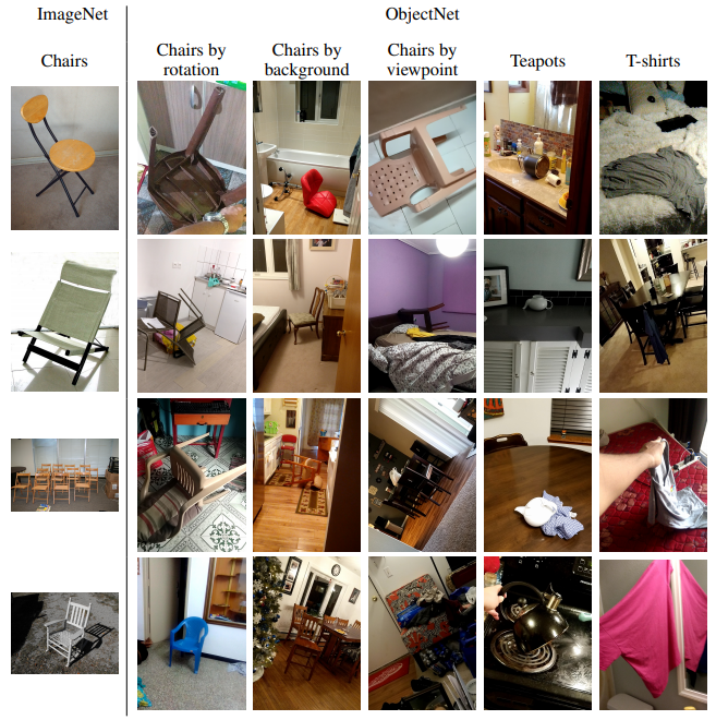
We use as outliers corrupted variants of CIFAR10 and CIFAR100 [18], as well as a scenario where ImageNet [9] is used as ID data and ObjectNet [2] as OOD, both resized to 32x32. Figure 10 shows samples from these data sets. The Gram and nnPU baselines do not give satisfactory results on the difficult CIFAR10/CIFAR100 settings in Table 1 and thus we do not consider them for the covariate shift cases. For the SSND methods (e.g. MCD, Mahal-U and ERD/ERD++) we evaluate on the same unlabeled set that is used for training (see the discussion in Section F.1).

Figure 10: Left: Samples from ImageNet and ObjectNet taken from the original paper by [2]. Right: Data samples for the corrupted CIFAR10-C data set.

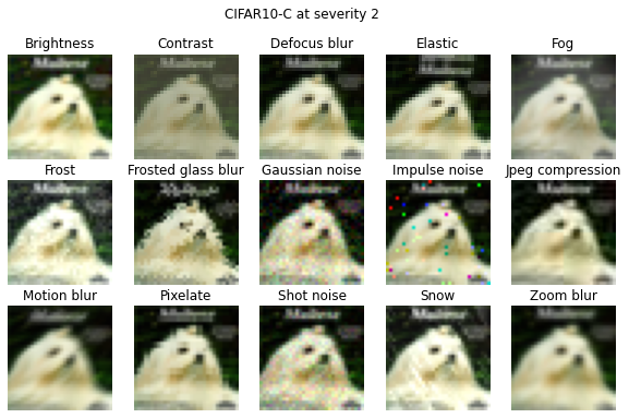
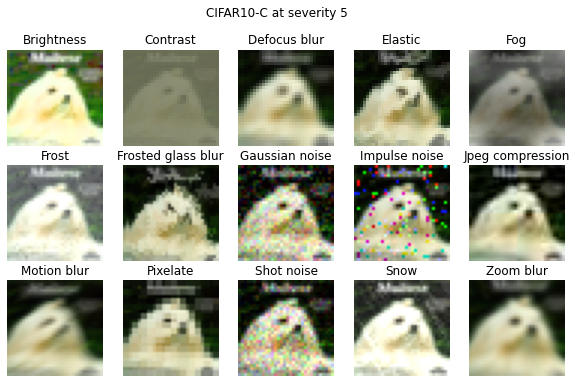
Furthermore, we present results on distinguishing between CIFAR10 [25] and CIFAR10v2 [39], a data set meant to be drawn from the same distribution as CIFAR10 (generated from the Tiny Images collection). In recht [39], the authors argue that CIFAR10 and CIFAR10v2 come from very similar distributions. They provide supporting evidence by training a binary classifier to distinguish between them, and observing that the accuracy that is obtained of 52.9% is very close to random.

Our experiments show that the two data sets are actually distinguishable, contrary to what previous work has argued. First, our own binary classifier trained on CIFAR10 vs CIFAR10v2 obtains a test accuracy of 67%, without any hyperparameter tuning. The model we use is a ResNet20 trained for 200 epochs using SGD with momentum 0.9. The learning rate is decayed by 0.2 at epochs 90, 140, 160 and 180. We use 1600 examples from each data set for training, and we validate using 400 examples from each data set.

Table 7: OOD detection performance on CIFAR10 vs CIFAR10v2

ID data	OOD data	Vanilla Ensembles	DPN	OE	Mahal.	MCD	Mahal-U	ERD	ERD++
		AUROC $\uparrow$ / TNR@95 $\uparrow$
CIFAR10	CIFAR10v2	0.64 / 0.13	0.63 / 0.09	0.64 / 0.12	0.55 / 0.08	0.58 / 0.10	0.56 / 0.07	0.76 / 0.26	0.91 / 0.80

Our OOD detection experiments (presented in Table 7) show that most baselines are able to distinguish between the two data sets, with ERD achieving the highest performance. The methods which require OOD data for tuning (Outlier Exposure and DPN) use CIFAR100.

Table 8: OOD detection performance on data with covariate shift. For ERD and vanilla ensembles, we train 5 ResNet20 models for each setting. The evaluation metrics are computed on the unlabeled set.

ID data	OOD data	Vanilla Ensembles	DPN	OE	Mahal.	MCD	Mahal-U	ERD	ERD++
		AUROC $\uparrow$ / TNR@95 $\uparrow$
CIFAR10	CIFAR10-C sev 2 (A)	0.68 / 0.20	0.73 / 0.31	0.70 / 0.20	0.84 / 0.53	0.82 / 0.50	0.75 / 0.38	0.96 / 0.86	0.99 / 0.95
CIFAR10	CIFAR10-C sev 2 (W)	0.51 / 0.05	0.47 / 0.03	0.52 / 0.06	0.58 / 0.08	0.52 / 0.06	0.55 / 0.07	0.68 / 0.19	0.86 / 0.41
CIFAR10	CIFAR10-C sev 5 (A)	0.84 / 0.49	0.89 / 0.60	0.86 / 0.54	0.94 / 0.80	0.95 / 0.84	0.88 / 0.63	1.00 / 0.99	1.00 / 1.00
CIFAR10	CIFAR10-C sev 5 (W)	0.60 / 0.10	0.72 / 0.10	0.63 / 0.11	0.78 / 0.27	0.60 / 0.08	0.68 / 0.12	0.98 / 0.86	1.00 / 1.00
CIFAR100	CIFAR100-C sev 2 (A)	0.68 / 0.20	0.62 / 0.18	0.65 / 0.19	0.82 / 0.48	0.72 / 0.29	0.67 / 0.22	0.94 / 0.76	0.97 / 0.86
CIFAR100	CIFAR100-C sev 2 (W)	0.52 / 0.06	0.32 / 0.03	0.52 / 0.06	0.55 / 0.07	0.52 / 0.06	0.55 / 0.06	0.71 / 0.19	0.86 / 0.44
CIFAR100	CIFAR100-C sev 5 (A)	0.78 / 0.37	0.74 / 0.36	0.76 / 0.37	0.92 / 0.72	0.91 / 0.65	0.84 / 0.55	0.99 / 0.97	1.00 / 0.99
CIFAR100	CIFAR100-C sev 5 (W)	0.64 / 0.14	0.49 / 0.12	0.62 / 0.13	0.71 / 0.19	0.60 / 0.10	0.63 / 0.13	0.96 / 0.71	0.98 / 0.89
Tiny ImageNet	Tiny ObjectNet	0.82 / 0.49	0.70 / 0.32	0.79 / 0.37	0.75 / 0.26	0.99 / 0.98	0.72 / 0.25	0.98 / 0.88	0.99 / 0.98
Average		0.67 / 0.23	0.63 / 0.23	0.67 / 0.23	0.76 / 0.38	0.74 / 0.39	0.70 / 0.27	0.91 / 0.71	0.96 / 0.83

F.5 Results with a smaller unlabeled set

We now show that our method performs well even when the unlabeled set is significantly smaller. In particular, we show in the table below that ERD maintains a high AUROC and TNR@95 even when only 1,000 unlabeled samples are used for fine-tuning (500 ID and 500 OOD).

Table 9: Experiments with a test set of size 1,000, with an equal number of ID and OOD test samples. For ERD and vanilla ensembles, we train 5 ResNet20 models for each setting. The evaluation metrics are computed on the unlabeled set.

ID data	OOD data	Vanilla Ensembles	DPN	OE	Mahal.	MCD	Mahal-U	ERD
		AUROC $\uparrow$ / TNR@95 $\uparrow$
SVHN	CIFAR10	0.97 / 0.88	1.00 / 1.00	1.00 / 1.00	0.99 / 0.98	0.97 / 0.85	0.99 / 0.95	1.00 / 0.99
CIFAR10	SVHN	0.92 / 0.78	0.95 / 0.85	0.97 / 0.89	0.99 / 0.96	1.00 / 0.98	0.99 / 0.96	1.00 / 1.00
CIFAR100	SVHN	0.84 / 0.48	0.77 / 0.44	0.82 / 0.50	0.98 / 0.90	0.97 / 0.73	0.98 / 0.92	0.99 / 1.00
SVHN[0:4]	SVHN[5:9]	0.92 / 0.69	0.87 / 0.19	0.85 / 0.52	0.92 / 0.71	0.91 / 0.51	0.91 / 0.63	0.97 / 0.86
CIFAR10[0:4]	CIFAR10[5:9]	0.80 / 0.39	0.82 / 0.32	0.82 / 0.41	0.79 / 0.27	0.69 / 0.25	0.64 / 0.13	0.87 / 0.50
CIFAR100[0:49]	CIFAR100[50:99]	0.78 / 0.35	0.70 / 0.26	0.74 / 0.31	0.72 / 0.20	0.70 / 0.26	0.72 / 0.19	0.79 / 0.38
CIFAR10	CIFAR10-C sev 2 (A)	0.68 / 0.20	0.73 / 0.31	0.70 / 0.20	0.84 / 0.53	0.82 / 0.50	0.75 / 0.38	0.91 / 0.71
CIFAR10	CIFAR10-C sev 2 (W)	0.51 / 0.05	0.47 / 0.03	0.52 / 0.06	0.58 / 0.08	0.52 / 0.06	0.55 / 0.07	0.57 / 0.09
CIFAR10	CIFAR10-C sev 5 (A)	0.84 / 0.49	0.89 / 0.60	0.86 / 0.54	0.94 / 0.80	0.95 / 0.84	0.88 / 0.63	0.99 / 0.95
CIFAR10	CIFAR10-C sev 5 (W)	0.60 / 0.10	0.72 / 0.10	0.63 / 0.11	0.78 / 0.27	0.60 / 0.08	0.68 / 0.12	0.92 / 0.67
CIFAR100	CIFAR100-C sev 2 (A)	0.68 / 0.20	0.62 / 0.18	0.65 / 0.19	0.82 / 0.48	0.72 / 0.29	0.67 / 0.22	0.84 / 0.48
CIFAR100	CIFAR100-C sev 2 (W)	0.52 / 0.06	0.32 / 0.03	0.52 / 0.06	0.55 / 0.07	0.52 / 0.06	0.55 / 0.06	0.55 / 0.07
CIFAR100	CIFAR100-C sev 5 (A)	0.78 / 0.37	0.74 / 0.36	0.76 / 0.37	0.92 / 0.72	0.91 / 0.65	0.84 / 0.55	0.96 / 0.80
CIFAR100	CIFAR100-C sev 5 (W)	0.64 / 0.14	0.49 / 0.12	0.62 / 0.13	0.71 / 0.19	0.60 / 0.10	0.63 / 0.13	0.81 / 0.25
Average		0.75 / 0.37	0.72 / 0.34	0.75 / 0.38	0.82 / 0.51	0.78 / 0.44	0.77 / 0.42	0.87 / 0.62

F.6 More results for Outlier Exposure

The Outlier Exposure method needs access to a set of OOD samples during training. The numbers we report in the rest of paper for Outlier Exposure are obtained by using the TinyImages data set as the OOD samples that are seen during training. In this section we explore the use of an OOD${}_{\text{train}}$ data set that is more similar to the OOD data observed at test time. This is a much easier setting for the Outlier Exposure method: the closer OOD${}_{\text{train}}$ is to OOD${}_{\text{test}}$, the easier it will be for the model tuned on OOD${}_{\text{train}}$ to detect the test OOD samples.

In the table below we focus only on the settings with corruptions. For each corruption type, we use the lower severity corruption as OOD${}_{\text{train}}$ and evaluate on the higher severity data and vice versa. We report for each metric the average taken over all corruptions (A), and the value for the worst-case setting (W).

ID data	OOD data	OE (trained on sev5)	OE (trained on sev2)
		AUROC $\uparrow$
CIFAR10	CIFAR10-C sev 2 (A)	0.89	N/A
CIFAR10	CIFAR10-C sev 2 (W)	0.65	N/A
CIFAR10	CIFAR10-C sev 5 (A)	N/A	0.98
CIFAR10	CIFAR10-C sev 5 (W)	N/A	0.78
CIFAR100	CIFAR100-C sev 2 (A)	0.85	N/A
CIFAR100	CIFAR100-C sev 2 (W)	0.59	N/A
CIFAR100	CIFAR100-C sev 5 (A)	N/A	0.97
CIFAR100	CIFAR100-C sev 5 (W)	N/A	0.67
Average		0.87	0.98

Table 10: Results for Outlier Exposure, when using the same corruption type, but with a higher/lower severity, as OOD data seen during training.

F.7 Results on MNIST and FashionMNIST

Table 11: Results on MNIST/FashionMNIST settings. For ERD and vanilla ensembles, we train 5 3-hidden layer MLP models for each setting. The evaluation metrics are computed on the unlabeled set.

ID data	OOD data	Vanilla Ensembles	DPN	OE	Mahal.	nnPU	MCD	Mahal-U	Bin. Classif.	ERD	ERD++
		AUROC $\uparrow$ / TNR@95 $\uparrow$
MNIST	FMNIST	0.81 / 0.01	1.00 / 1.00	1.00 / 1.00	1.00 / 1.00	1.00 / 1.00	1.00 / 0.98	1.00 / 1.00	1.00 / 1.00	1.00 / 1.00	1.00 / 1.00
FMNIST	MNIST	0.87 / 0.42	1.00 / 1.00	0.68 / 0.16	0.99 / 0.97	1.00 / 1.00	1.00 / 1.00	0.99 / 0.96	1.00 / 1.00	1.00 / 1.00	1.00 / 1.00
MNIST[0:4]	MNIST[5:9]	0.94 / 0.72	0.99 / 0.97	0.95 / 0.78	0.99 / 0.98	0.99 / 0.97	0.96 / 0.76	0.99 / 0.98	0.99 / 0.94	0.99 / 0.96	0.99 / 0.97
FMNIST[0,2,3,7,8]	FMNIST[1,4,5,6,9]	0.64 / 0.07	0.77 / 0.15	0.66 / 0.12	0.77 / 0.20	0.95 / 0.71	0.78 / 0.30	0.82 / 0.39	0.95 / 0.66	0.94 / 0.67	0.94 / 0.68
Average		0.82 / 0.30	0.94 / 0.78	0.82 / 0.51	0.94 / 0.79	0.98 / 0.92	0.94 / 0.76	0.95 / 0.83	0.98 / 0.90	0.98 / 0.91	0.98 / 0.91

For FashionMNIST we chose this particular split (i.e. classes 0,2,3,7,8 vs classes 1,4,5,6,9) because the two partitions are more similar to each other. This makes novelty detection more difficult than the 0-4 vs 5-9 split.

F.8 Vanilla and ERD Ensembles with different architectures

In this section we present OOD detection results for 5-model Vanilla and ERD ensembles with different architecture choices, and note that the better performance of our method is maintained across model classes. Moreover, we observe that ERD benefits from employing more complex models, like the WideResNet.

Table 12: Results with three different architectures for Vanilla and ERD ensembles. All ensembles comprise 5 models. For the corruption data sets, we report for each metric the average taken over all corruptions (A), and the value for the worst-case setting (W). The evaluation metrics are computed on the unlabeled set.

		VGG16		ResNet20		WideResNet-28-10
ID data	OOD data	Vanilla Ensembles	ERD	Vanilla Ensembles	ERD	Vanilla Ensembles	ERD
		AUROC $\uparrow$ / TNR@95 $\uparrow$
SVHN	CIFAR10	0.97 / 0.88	0.99 / 0.94	0.97 / 0.88	0.99 / 0.97	0.96 / 0.86	1.00 / 0.99
CIFAR10	SVHN	0.88 / 0.69	1.00 / 1.00	0.92 / 0.78	1.00 / 1.00	0.94 / 0.81	1.00 / 1.00
SVHN[0:4]	SVHN[5:9]	0.89 / 0.60	0.93 / 0.63	0.92 / 0.69	0.94 / 0.66	0.91 / 0.62	0.96 / 0.78
CIFAR10[0:4]	CIFAR10[5:9]	0.74 / 0.29	0.91 / 0.63	0.80 / 0.39	0.91 / 0.66	0.80 / 0.35	0.94 / 0.71
CIFAR10	CIFAR10-C sev 2 (A)	0.66 / 0.17	0.94 / 0.79	0.68 / 0.20	0.96 / 0.86	0.69 / 0.18	0.98 / 0.90
CIFAR10	CIFAR10-C sev 2 (W)	0.51 / 0.05	0.68 / 0.19	0.51 / 0.05	0.68 / 0.19	0.51 / 0.05	0.84 / 0.35
CIFAR10	CIFAR10-C sev 5 (A)	0.80 / 0.41	0.99 / 0.96	0.84 / 0.49	1.00 / 0.99	0.84 / 0.47	1.00 / 1.00
CIFAR10	CIFAR10-C sev 5 (W)	0.58 / 0.10	0.95 / 0.72	0.60 / 0.10	0.98 / 0.86	0.59 / 0.09	0.99 / 0.97
Average		0.75 / 0.40	0.92 / 0.73	0.78 / 0.45	0.93 / 0.77	0.78 / 0.43	0.96 / 0.84

F.9 Impact of the ensemble size and of the choice of arbitrary label

In this section we show novelty detection results with our method using a smaller number of models for the ensembles. We notice that the performance is not affected substantially, indicating that the computation cost of our approach could be further reduced by fine-tuning smaller ensembles.

Table 13: Results obtained with smaller ensembles for ERD. The numbers for $K<5$ are averages over 3 runs, where we use a different set of arbitrary labels for each run to illustrate our method’s stability with respect the choice of labels to be assigned to the unlabeled set. We note that the standard deviations are small ($\sigma\leq 0.01$ for the AUROC values and $\sigma\leq 0.08$ for the TNR@95 values).

		K=2		K=3		K=4		K=5
ID data	OOD data	ERD	ERD++	ERD	ERD++	ERD	ERD++	ERD	ERD++
		AUROC $\uparrow$ / TNR@95 $\uparrow$
SVHN	CIFAR10	0.99 / 0.98	0.99 / 0.99	0.99 / 0.98	1.00 / 0.99	0.99 / 0.98	1.00 / 0.99	1.00 / 0.99	1.00 / 0.99
CIFAR10	SVHN	1.00 / 1.00	1.00 / 1.00	1.00 / 1.00	1.00 / 1.00	1.00 / 1.00	1.00 / 1.00	1.00 / 1.00	1.00 / 1.00
CIFAR100	SVHN	1.00 / 1.00	1.00 / 1.00	1.00 / 1.00	1.00 / 1.00	1.00 / 1.00	1.00 / 1.00	1.00 / 1.00	1.00 / 1.00
SVHN[0:4]	SVHN[5:9]	0.95 / 0.69	0.94 / 0.68	0.95 / 0.73	0.95 / 0.75	0.96 / 0.76	0.96 / 0.77	0.95 / 0.74	0.96 / 0.77
CIFAR10[0:4]	CIFAR10[5:9]	0.89 / 0.55	0.92 / 0.58	0.89 / 0.57	0.94 / 0.70	0.90 / 0.57	0.95 / 0.73	0.93 / 0.70	0.96 / 0.79
CIFAR100[0:49]	CIFAR100[50:99]	0.81 / 0.40	0.82 / 0.43	0.81 / 0.41	0.84 / 0.44	0.81 / 0.41	0.84 / 0.44	0.82 / 0.44	0.85 / 0.45
Average		0.94 / 0.77	0.95 / 0.78	0.94 / 0.78	0.95 / 0.81	0.94 / 0.79	0.96 / 0.82	0.95 / 0.81	0.96 / 0.83

Impact of the choice of arbitrary labels.

Furthermore, we note that in the table we report averages over 3 runs of our method, where for each run we use a different subset of $\mathcal{Y}$ to assign arbitrary labels to the unlabeled data. We do this in order to assess the stability of ERD ensembles to the choice of the arbitrary labels and notice that the novelty detection performance metrics do not vary significantly. Concretely, the standard deviations are consistently below $0.01$ for all data sets for the AUROC metric, and below $0.07$ for the TNR@95 metric.

F.10 Detection performance on different OOD data

In this section we investigate whether the proposed method maintains its good novelty detection performance when the test-time OOD data comes from a different data set compared to the OOD data that is present in the unlabeled set used for fine-tuning. In particular, we are interested if our approach can still identify outliers in situations when they suffer from various corruptions. This scenario can sometimes occur in practice, when machine failure or uncurated data can lead to mild distribution shift.

Concretely, we focus on the difficult near OOD scenarios and take as ID half of the CIFAR10 or CIFAR100 classes, while the other half is OOD. For this experiment, we fine-tune the ERD ensembles using clean OOD data from the other half of CIFAR10 and CIFAR100, respectively. For evaluation, we use clean ID data and corrupted OOD samples from CIFAR10-C and CIFAR100-C, respectively. We give more details on these corrupted data sets in Appendix F.4. We consider corruptions of severity 2 and 5 from all corruptions types.

In Table 14 we show the average AUROC and the worst AUROC over all corruption types for vanilla and ERD ensembles. Note that our approach maintains a similar performance compared to the numbers presented in Table 1 for same test-time OOD data. It is also noteworthy that all the average AUROC values are consistently larger than the baselines in Table 1.

Table 14: Results obtained when evaluating on an OOD data set different from the one used for fine-tuning. All ERD ensembles are tuned on clean ID and OOD data and are evaluated on OOD data with corruptions.

ID data	OOD data in unlabeled set	Test-time OOD data	Vanilla Ensemble	ERD
			AUROC $\uparrow$
CIFAR10[0:4]	CIFAR10[5:9]	CIFAR10[5:9]-C sev 2 (A)	0.82	0.93
CIFAR10[0:4]	CIFAR10[5:9]	CIFAR10[5:9]-C sev 2 (W)	0.77	0.88
CIFAR10[0:4]	CIFAR10[5:9]	CIFAR10[5:9]-C sev 5 (A)	0.85	0.91
CIFAR10[0:4]	CIFAR10[5:9]	CIFAR10[5:9]-C sev 5 (W)	0.79	0.86
CIFAR100[0:49]	CIFAR100[50:99]	CIFAR100[50:99]-C sev 2 (A)	0.78	0.84
CIFAR100[0:49]	CIFAR100[50:99]	CIFAR100[50:99]-C sev 2 (W)	0.75	0.78
CIFAR100[0:49]	CIFAR100[50:99]	CIFAR100[50:99]-C sev 5 (A)	0.77	0.83
CIFAR100[0:49]	CIFAR100[50:99]	CIFAR100[50:99]-C sev 5 (W)	0.63	0.78

Appendix G Medical OOD detection benchmark

The medical OOD detection benchmark is organized as follows. There are four training (ID) data sets, from three different domains: two data sets with chest X-rays, one with fundus imaging and one with histology images. For each ID data set, the authors consider three different OOD scenarios:

1. Use case 1: The OOD data set contains images from a completely different domain, similar to our category of easy OOD detection settings.

2. Use case 2: The OOD data set contains images with various corruptions, similar to the hard covariate shift settings that we consider in Section F.4.

3. Use case 3: The OOD data set contains images that come from novel classes, not seen during training.

Figure 11: Samples from the medical image benchmark. There are 3 ID data sets containing frontal and lateral chest X-rays and retinal images. Hard OOD samples contain images of diseases that are not present in the training set.

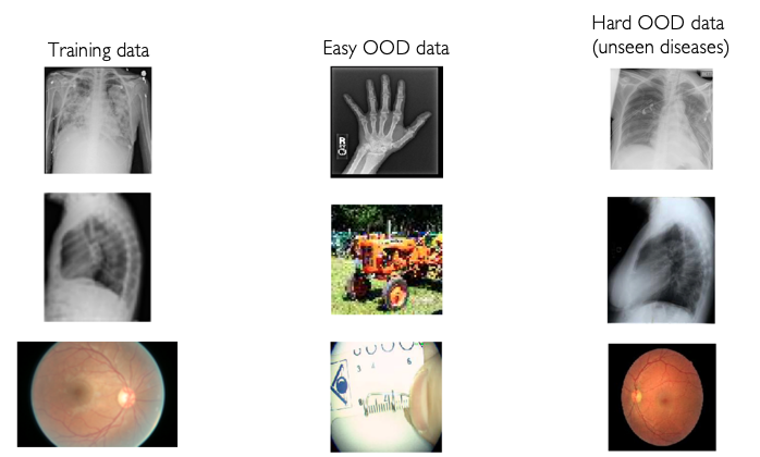
The authors evaluate a number of methods on all these scenarios. The methods can be roughly categorized as follows:

1. Data-only methods: Fully non-parametric approaches like kNN.

2. Classifier-only methods: Methods that use a classifier trained on the training set, e.g. ODIN [30], Mahalanobis [28]. ERD falls into this category as well.

3. Methods with Auxiliary Models: Methods that use an autoencoder or a generative model, like a Variational Autoencoder or a Generative Adversarial Network. Some of these approaches can be expensive to train and difficult to optimize and tune.

We stress the fact that for most of these methods the authors use (known) OOD data during training. Oftentimes the OOD samples observed during training come from a data set that is very similar to the OOD data used for evaluation. For exact details regarding the data sets and the methods used for the benchmark, we refer the reader to Cao2020 [6].

Figure 12: AUROC averaged over all scenarios in the medical OOD detection benchmark [6]. The values for all the baselines are computed using code made available by the authors of Cao2020 [6]. Notably, most of the baselines assume oracle knowledge of OOD data at training time.

Figure 13: AUROC averaged over the novel-class scenarios in the medical OOD detection benchmark [6], i.e. only use case 3.

In addition, in Figure 13 we present the average taken over only the novel-class settings in the medical benchmark. We observe that the performance of all methods is drastically affected, all of them performing much worse than the average presented in Figure 12. This stark decrease in AUROC and TNR@95 indicates that novelty detection is indeed a challenging task for OOD detection methods even in realistic settings. Nevertheless, 2-model ERD ensembles maintain a better performance than the baselines.

In Figures 14, 15, 16 we present AUROC and AUPR (Area under the Precision Recall curve) for ERD for each of the training data sets, and each of the use cases. Figure 12 presents averages over all settings that we considered, for all the baseline methods in the benchmark. Notably, ERD performs well consistently across data sets. The baselines are ordered by their average performance on all the settings (see Figure 12).

For all medical benchmarks, the unlabeled set is balanced, with an equal number of ID and OOD samples (subsampling the bigger data set, if necessary). We use the unlabeled set for evaluation.

Figure 14: Comparison between ERD and the various baselines on the NIH chest X-ray data set, for use case 1 (top), use case 2 (middle) and use case 3 (bottom). Baselines ordered as in Figure 12.

Figure 15: Comparison between ERD and the various baselines on the PC chest X-ray data set, for use case 1 (top), use case 2 (middle) and use case 3 (bottom). Baselines ordered as in Figure 12.

Figure 16: Comparison between ERD and the various baselines on the DRD fundus imaging data set, for use case 1 (top), use case 2 (middle) and use case 3 (bottom). Baselines ordered as in Figure 12.

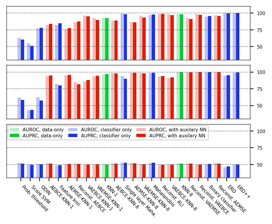
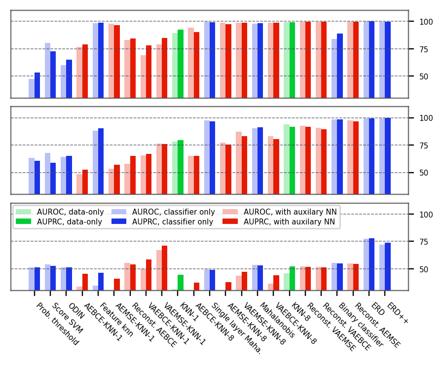
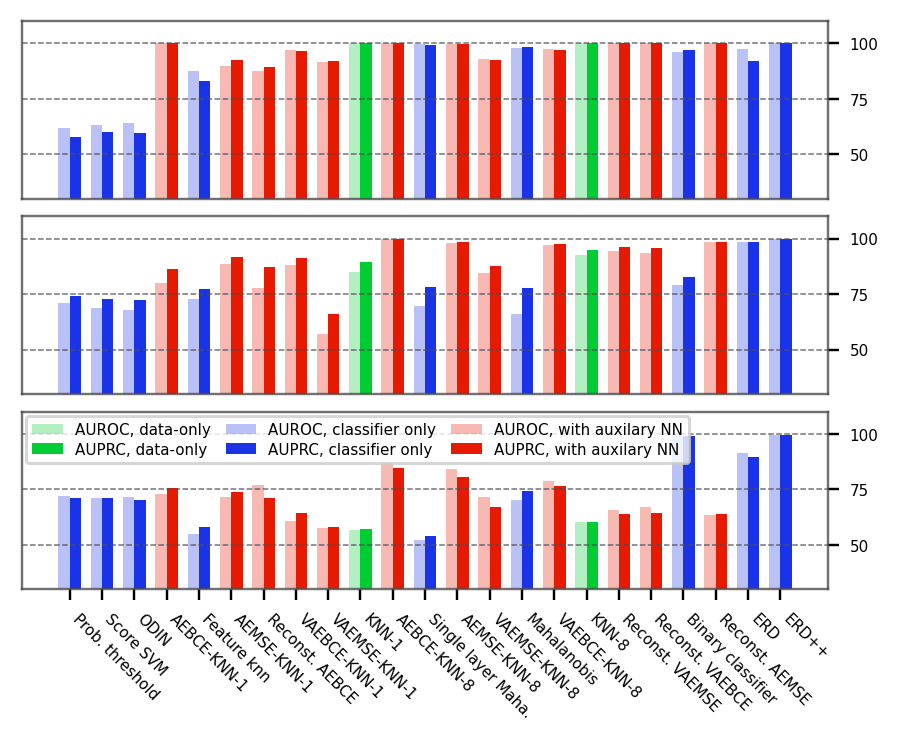
Appendix H Effect of learning rate and batch size

We show now that ERD ensembles are not too sensitive to the choice of hyperparameters. We illustrate this by varying the learning rate and the batch size, the hyperparameters that we identify as most impactful. As Figure 17 shows, many different configurations lead to similar novelty detection performance.

Figure 17: AUROCs obtained with an ensemble of WRN-28-10 models, as the initial learning rate and the batch size are varied. We used the hardest setting, CIFAR100:0-50 as ID, and CIFAR100:50-100 as OOD.

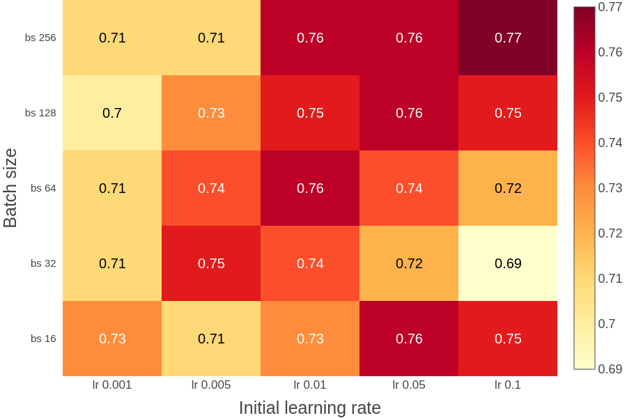
Appendix I Additional figure showing the dependence on the unlabeled set configuration

The configuration of the unlabeled set (i.e. the size of the unlabeled set, the ratio of OOD samples in the unlabeled set) influences the performance of our method, as illustrated in Figure 5(b). Below, we show that the same trend persists for different data sets too, e.g. when we consider CIFAR10 as ID data and SVHN as OOD data.

Figure 18: The AUROC of a 3-model ERD ensemble as the number and proportion of ID (CIFAR10) and OOD (SVHN) samples in the unlabeled set are varied.

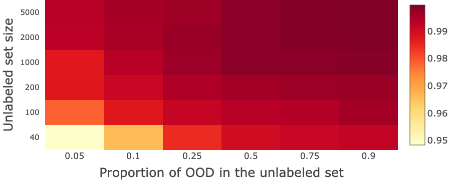
Appendix J Learning curves for other data sets

In addition to Figure 4, we present in this section learning curves for other data sets as well. The trend that persists throughout all figures is that the arbitrary label is learned first on the unlabeled OOD data. Choosing a stopping time before the validation accuracy starts to deteriorate prevents the model from fitting the arbitrary label on unlabeled ID data.

Impact of near OOD data on training ERD ensembles.

The learning curves illustrated in Figure 19 provide insight into what happens when the OOD data is similar to the ID training samples and the impact that has on training the proposed method. In particular, notice that for CIFAR10[0-4] vs CIFAR10[5-9] in Figure 19(d), the models require more training epochs before reaching an accuracy on unlabeled OOD samples of 100%. The learning of the arbitrary label on the OOD samples is delayed by the fact that the ID and OOD data are similar, and hence, the bias of the correctly labeled training set has a strong effect on the predictions of the models on the OOD inputs. Since we early stop when the validation accuracy starts deteriorating (e.g. at around epoch $8$ in Figure 19(d)), we end up using models that do not interpolate the arbitrary label on the OOD samples. Therefore, the ensemble does not disagree on the entirety of the OOD data in the unlabeled set, which leads to lower novelty detection performance. Importantly, however, our empirical evaluation reveals that the drop in performance for ERD ensembles is substantially smaller than what we observe for other OOD detection methods, even on near OOD data sets.

(a) ID = SVHN; OOD = CIFAR10.

(b) ID = SVHN[0-4]; OOD = SVHN[5-9].

(c) ID = CIFAR10; OOD = SVHN.

(d) ID = CIFAR10[0-4]; OOD = CIFAR10[5-9].

(e) ID = CIFAR100; OOD = SVHN.

(f) ID = CIFAR100[0-49]; OOD = CIFAR100[50-99].

Figure 19: Accuracy measured while fine-tuning a model pretrained on $S$ (epoch 0 indicates values obtained with the initial pretrained weights). The samples in $(U_{\mathrm{OOD}},c)$ are fit first, while the model reaches high accuracy on $(U_{\mathrm{ID}},c)$ much later. We fine-tune for at least one epoch and then early stop when the validation accuracy starts decreasing.

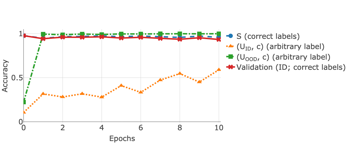
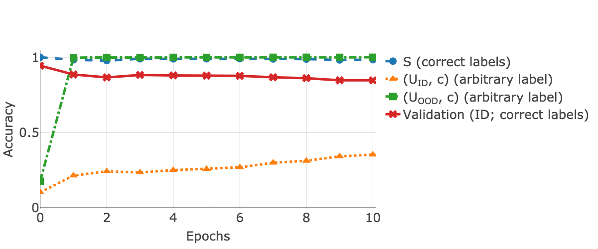
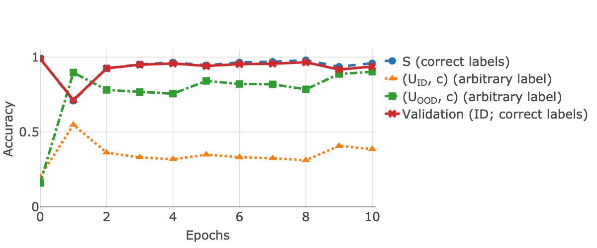
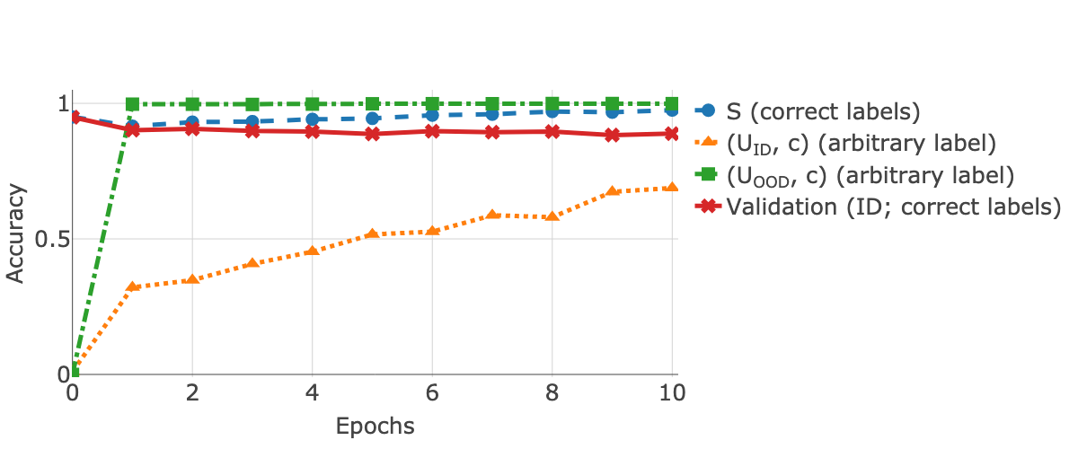
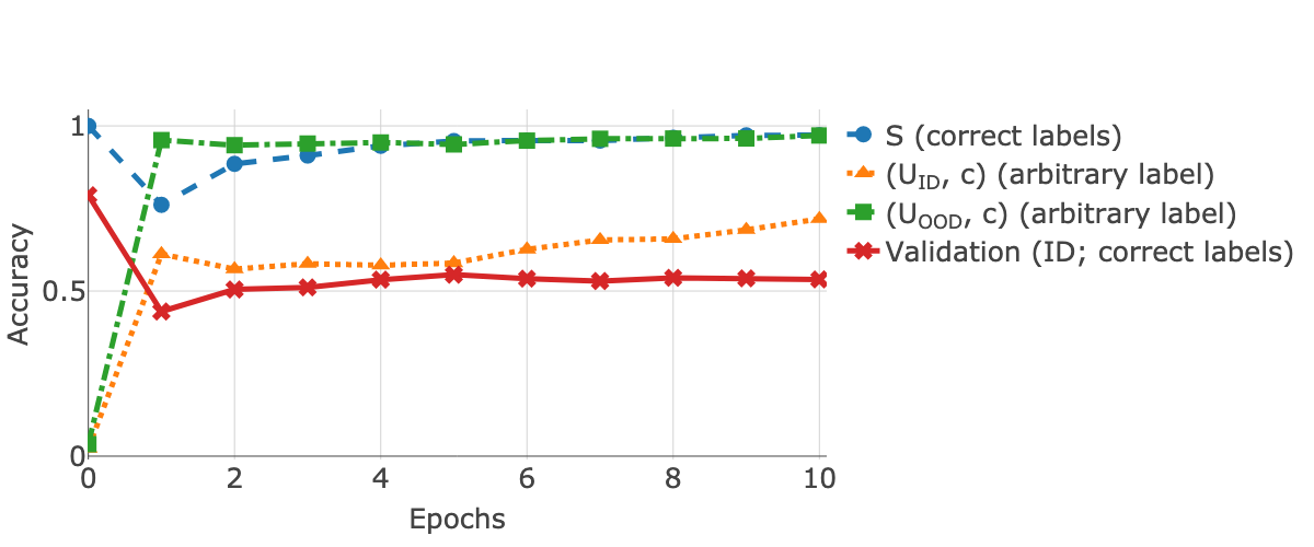
Appendix K Evolution of disagreement score during fine-tuning

In this section we illustrate how the distribution of the disagreement score changes during fine-tuning for ID and OOD data, for a 5-model ERD ensemble. Thus, we can further understand why the performance of the ERD ensembles is impacted by near OOD data.

Figure 20 reveals that for far OOD data (the left column) the disagreement scores computed on OOD samples are well separated from the disagreement scores on ID data (note that disagreement on OOD data is so concentrated around the maximum value of $2$ that the boxes are essentially reduced to a line segment). On the other hand, for near OOD data (the right column) there is sometimes significant overlap between the disagreement scores on ID and OOD data, which leads to the slightly lower AUROC values that we report in Table 1.

The figures also illustrate how the disagreement on the ID data tends to increase as we fine-tune the ensemble for longer, as a consequence of the models fitting the arbitrary labels on the unlabeled ID samples. Conversely, in most instances one epoch suffices for fitting the arbitrary label on the OOD data.

We need to make one important remark: While in the figure we present disagreement scores for the ensemble obtained after each epoch of fine-tuning, we stress that the final ERD ensemble need not be selected among these. In particular, since each model for ERD is early stopped separately, potentially at a different iteration, it is likely that the ERD ensemble contains models fine-tuned for a different number of iterations. Since we select the ERD ensembles from a strictly larger set, the final ensemble selected by the our proposed approach will be at least as good at distinguishing ID and OOD data as the best ensemble depicted in Figure 20.

(a) ID = SVHN; OOD = CIFAR10.

(b) ID = SVHN[0-4]; OOD = SVHN[5-9].

(c) ID = CIFAR10; OOD = SVHN.

(d) ID = CIFAR10[0-4]; OOD = CIFAR10[5-9].

(e) ID = CIFAR100; OOD = SVHN.

(f) ID = CIFAR100[0-49]; OOD = CIFAR100[50-99].

Figure 20: The distribution of the disagreement score measured during fine-tuning on ID and OOD data (blue and orange boxes, respectively). The box indicates the lower and upper quartiles of the distribution, while the middle line represents the median and the whiskers show the extreme values. Notice that the distributions of the scores are easier to distinguish for far OOD data (left column), and tend to overlap more for near OOD settings (right column).

References

- [1] S. Akçay, A. Atapour-Abarghouei, and T. Breckon. GANomaly: Semi-supervised anomaly detection via adversarial training. In ACCV, 2018.
- [2] A. Barbu, D. Mayo, J. Alverio, W. Luo, C. Wang, D. Gutfreund, J. Tenenbaum, and B. Katz. ObjectNet: A large-scale bias-controlled dataset for pushing the limits of object recognition models. In Advances in Neural Information Processing Systems 32, pages 9453–9463. 2019.
- [3] K. P. Bennett, A. Demiriz, and R. Maclin. Exploiting unlabeled data in ensemble methods. Proceedings of the eighth ACM SIGKDD international conference on Knowledge discovery and data mining, 2002.
- [4] S. Bulusu, B. Kailkhura, B. Li, P. K. Varshney, and D. Song. Anomalous instance detection in deep learning: A survey. arXiv preprint arXiv:2003.06979, 2020.
- [5] E. Calli, E. Sogancioglu, B. van Ginneken, K. G. van Leeuwen, and K. Murphy. Deep learning for chest X-ray analysis: A survey. Medical Image Analysis, 2021.
- [6] T. Cao, C.-W. Huang, D. Y.-T. Hui, and J. P. Cohen. A benchmark of medical out of distribution detection. arXiv preprint arXiv:2007.04250, 2020.
- [7] Q. Da, Y. Yu, and Z.-H. Zhou. Learning with augmented class by exploiting unlabeled data. In AAAI, 2014.
- [8] T. Daniel, T. Kurutach, and A. Tamar. Deep variational semi-supervised novelty detection. arXiv preprint arXiv:1911.04971, 2019.
- [9] J. Deng, W. Dong, R. Socher, L.-J. Li, K. Li, and L. Fei-Fei. ImageNet: A large-scale hierarchical image database. In Proceedings of the IEEE Conference on Computer Vision and Pattern Recognition (CVPR), 2009.
- [10] M. C. du Plessis, G. Niu, and M. Sugiyama. Analysis of learning from positive and unlabeled data. In Advances in Neural Information Processing Systems 27, 2014.
- [11] S. Fort, J. Ren, and B. Lakshminarayanan. Exploring the limits of out-of-distribution detection. arXiv preprint arXiv:2106.03004, 2021.
- [12] Y. Gal and Z. Ghahramani. Dropout as a Bayesian approximation: Representing model uncertainty in deep learning. volume 48 of Proceedings of Machine Learning Research, pages 1050–1059, 2016.
- [13] C. Geng, S.-J. Huang, and S. Chen. Recent advances in open set recognition: A survey. IEEE Transactions on Pattern Analysis and Machine Intelligence, 43:3614–3631, 2021.
- [14] N. Gornitz, M. Kloft, K. Rieck, and U. Brefeld. Toward supervised anomaly detection. J. Artif. Int. Res., 46:235–262, 2013.
- [15] L.-Z. Guo, Z.-Y. Zhang, Y. Jiang, Y.-F. Li, and Z.-H. Zhou. Safe deep semi-supervised learning for unseen-class unlabeled data. In Proceedings of the 37th International Conference on Machine Learning, Proceedings of Machine Learning Research, pages 3897–3906, 2020.
- [16] D. Hafner, D. Tran, T. P. Lillicrap, A. Irpan, and J. Davidson. Noise contrastive priors for functional uncertainty. In UAI, 2019.
- [17] K. He, X. Zhang, S. Ren, and J. Sun. Deep residual learning for image recognition. In Proceedings of the IEEE Conference on Computer Vision and Pattern Recognition (CVPR), 2016.
- [18] D. Hendrycks and T. Dietterich. Benchmarking neural network robustness to common corruptions and perturbations. In Proceedings of the International Conference on Learning Representations, 2019.
- [19] D. Hendrycks and K. Gimpel. A baseline for detecting misclassified and out-of-distribution examples in neural networks. Proceedings of the International Conference on Learning Representations, 2017.
- [20] D. Hendrycks, M. Mazeika, and T. Dietterich. Deep anomaly detection with outlier exposure. In Proceedings of the International Conference on Learning Representations, 2019.
- [21] S. Jain, G. Liu, J. Mueller, and D. Gifford. Maximizing overall diversity for improved uncertainty estimates in deep ensembles. Proceedings of the AAAI Conference on Artificial Intelligence, 34:4264–4271, 2020.
- [22] I. Katsamenis, E. Protopapadakis, A. Voulodimos, A. Doulamis, and N. Doulamis. Transfer learning for COVID-19 pneumonia detection and classification in chest X-ray images. medRxiv, 2020.
- [23] P. Kirichenko, P. Izmailov, and A. G. Wilson. Why normalizing flows fail to detect out-of-distribution data. In Advances in Neural Information Processing Systems 33, pages 20578–20589, 2020.
- [24] R. Kiryo, G. Niu, M. C. du Plessis, and M. Sugiyama. Positive-unlabeled learning with non-negative risk estimator. In Advances in Neural Information Processing Systems 30, 2017.
- [25] A. Krizhevsky. Learning multiple layers of features from tiny images. Technical report, 2009.
- [26] B. Lakshminarayanan, A. Pritzel, and C. Blundell. Simple and scalable predictive uncertainty estimation using deep ensembles. In Advances in Neural Information Processing Systems 30, pages 6402–6413. 2017.
- [27] Y. Lecun, L. Bottou, Y. Bengio, and P. Haffner. Gradient-based learning applied to document recognition. In Proceedings of the IEEE, pages 2278–2324, 1998.
- [28] K. Lee, K. Lee, H. Lee, and J. Shin. A simple unified framework for detecting out-of-distribution samples and adversarial attacks. In Advances in Neural Information Processing Systems 31, pages 7167–7177. 2018.
- [29] M. Li, M. Soltanolkotabi, and S. Oymak. Gradient descent with early stopping is provably robust to label noise for overparameterized neural networks. Proceedings of Machine Learning Research, pages 4313–4324, 2020.
- [30] S. Liang, Y. Li, and R. Srikant. Enhancing the reliability of out-of-distribution image detection in neural networks. In Proceedings of the International Conference on Learning Representations, 2018.
- [31] H. Liu and P. Abbeel. Hybrid discriminative-generative training via contrastive learning. arXiv preprint arXiv:2007.09070, 2020.
- [32] S. Liu, R. Garrepalli, T. Dietterich, A. Fern, and D. Hendrycks. Open category detection with PAC guarantees. In Proceedings of the 35th International Conference on Machine Learning, pages 3169–3178, 2018.
- [33] S. Liu, J. Niles-Weed, N. Razavian, and C. Fernandez-Granda. Early-learning regularization prevents memorization of noisy labels. 2020.
- [34] A. Malinin and M. Gales. Predictive uncertainty estimation via prior networks. In Advances in Neural Information Processing Systems 32, page 7047–7058, 2018.
- [35] J. Mũnoz-Marí, F. Bovolo, L. Gómez-Chova, L. Bruzzone, and G. Camp-Valls. Semi-supervised one-class support vector machines for classification of remote sensing data. IEEE Transactions on Geoscience and Remote Sensing, 48:3188–3197, 2010.
- [36] E. Nalisnick, A. Matsukawa, Y. W. Teh, D. Gorur, and B. Lakshminarayanan. Do deep generative models know what they don’t know? In Proceedings of the International Conference on Learning Representations, 2019.
- [37] Y. Netzer, T. Wang, A. Coates, A. Bissacco, B. Wu, and A. Y. Ng. Reading digits in natural images with unsupervised feature learning. In NIPS Workshop on Deep Learning and Unsupervised Feature Learning 2011, 2011.
- [38] Y. Ovadia, E. Fertig, J. Ren, Z. Nado, D. Sculley, S. Nowozin, J. Dillon, B. Lakshminarayanan, and J. Snoek. Can you trust your model’s uncertainty? Evaluating predictive uncertainty under dataset shift. In Advances in Neural Information Processing Systems 32, pages 13991–14002. 2019.
- [39] B. Recht, R. Roelofs, L. Schmidt, and V. Shankar. Do ImageNet classifiers generalize to ImageNet? volume 97 of Proceedings of Machine Learning Research, pages 5389–5400, 2019.
- [40] J. Ren, S. Fort, J. Liu, A. G. Roy, S. Padhy, and B. Lakshminarayanan. A simple fix to Mahalanobis distance for improving near-OOD detection. arXiv preprint arXiv:2106.09022, 2021.
- [41] J. Ren, P. J. Liu, E. Fertig, J. Snoek, R. Poplin, M. Depristo, J. Dillon, and B. Lakshminarayanan. Likelihood ratios for out-of-distribution detection. In Advances in Neural Information Processing Systems 32, pages 14707–14718. 2019.
- [42] L. Ruff, R. A. Vandermeulen, N. Görnitz, A. Binder, E. Müller, K.-R. Müller, and M. Kloft. Deep semi-supervised anomaly detection. In Proceedings of the International Conference on Learning Representations, 2020.
- [43] C. S. Sastry and S. Oore. Detecting out-of-distribution examples with in-distribution examples and gram matrices. arXiv preprint arXiv:1912.12510, 2019.
- [44] C. Scott and G. Blanchard. Transductive anomaly detection. Technical report, 2008.
- [45] C. Scott and G. Blanchard. Novelty detection: Unlabeled data definitely help. In Proceedings of the Twelth International Conference on Artificial Intelligence and Statistics, volume 5, pages 464–471, 2009.
- [46] V. Sehwag, M. Chiang, and P. Mittal. {SSD}: A unified framework for self-supervised outlier detection. In International Conference on Learning Representations, 2021.
- [47] K. Sohn, C.-L. Li, J. Yoon, M. Jin, and T. Pfister. Learning and evaluating representations for deep one-class classification. In Proceedings of the International Conference on Learning Representations, 2021.
- [48] H. Song, Z. Jiang, A. Men, and B. Yang. A hybrid semi-supervised anomaly detection model for high-dimensional data. Computational Intelligence and Neuroscience, 2017.
- [49] H. Song, M. Kim, D. Park, and J.-G. Lee. How does early stopping help generalization against label noise? arXiv preprint arXiv:1911.08059, 2020.
- [50] J. Tack, S. Mo, J. Jeong, and J. Shin. CSI: Novelty detection via contrastive learning on distributionally shifted instances. In Advances in Neural Information Processing Systems 33, pages 11839–11852, 2020.
- [51] J. Winkens, R. Bunel, A. G. Roy, R. Stanforth, V. Natarajan, J. R. Ledsam, P. MacWilliams, P. Kohli, A. Karthikesalingam, S. Kohl, T. Cemgil, S. M. A. Eslami, and O. Ronneberger. Contrastive training for improved out-of-distribution detection. arXiv preprint arXiv:2007.05566, 2020.
- [52] H. Xiao, K. Rasul, and R. Vollgraf. Fashion-MNIST: A novel image dataset for benchmarking machine learning algorithms, 2017.
- [53] F. F. Yilmaz and R. Heckel. Image recognition from raw labels collected without annotators. arXiv preprint arXiv:1910.09055, 2019.
- [54] Q. Yu and K. Aizawa. Unsupervised out-of-distribution detection by maximum classifier discrepancy. In Proceedings of the IEEE/CVF International Conference on Computer Vision (ICCV), 2019.
- [55] H. Zhang, A. Li, J. Guo, and Y. Guo. Hybrid models for open set recognition. In ECCV, 2020.
- [56] M.-L. Zhang and Z.-H. Zhou. Exploiting unlabeled data to enhance ensemble diversity. Data Mining and Knowledge Discovery, 26:98–129, 2010.
- [57] Y.-J. Zhang, P. Zhao, L. Ma, and Z.-H. Zhou. An unbiased risk estimator for learning with augmented classes. In Advances in Neural Information Processing Systems, volume 33, pages 10247–10258, 2020.