New probability distributions in astrophysics: IV. The relativistic Maxwell-Boltzmann distribution

Abstract

Two relativistic distributions which generalizes the Maxwell Boltzman (MB) distribution are analyzed: the relativistic MB and the Maxwell-Jüttner (MJ) distribution. For the two distributions we derived in terms of special functions the constant of normalization, the average value, the second moment about the origin, the variance, the mode, the asymptotic behavior, approximate expressions for the average value as function of the temperature and the connected inverted expressions for the temperature as function of the average value. Two astrophysical applications to the synchrotron emission in presence of the magnetic field and the relativistic electrons are presented.

Keywords: 05.20.-y Classical statistical mechanics; 05.20.Dd Kinetic theory;

1 Introduction

The equivalent in special relativity (SR) of the Maxwell-Boltzmann (MB) distribution, see [1, 2], is the so called Maxwell-Jüttner distribution (MJ), see [3, 4]. The MJ distribution has been recently revisited, we select some approaches among others: a model for the anisotropic MJ distribution [6], an astrophysical application of the MJ distribution to the energy distribution in radio jets [7], a new family of MJ distributions characterized by the parameter $\eta$ [5] and an application to counter-streaming beams of charged particles [8]. The above approaches does not cover the determination of the statistical quantities of the MJ distribution. In this paper the statistical parameters of the relativistic MB distribution are derived in Section 2 and those of the MJ distribution are derived in Section 3. Section 4 derives the spectral synchrotron emissivity in the framework of the two relativistic distributions here analyzed.

2 The relativistic MB distribution

The usual MB distribution, $f(v;m,k,T_{MB})$, for an ideal gas is

$$f(v;m,k,T_{MB})=\frac{\sqrt{2}{v}^{2}{{\rm e}^{-\frac{1}{2}\,{\frac{{v}^{2}m}{kT_{MB}}}}}}{\sqrt{\pi}\left({\frac{kT_{MB}}{m}}\right)^{\frac{3}{2}}}\quad,$$ (1)

where $m$ is the mass of the gas molecules, $k$ is the Boltzmann constant and $T_{MB}$ is the usual thermodynamic temperature. In SR, the total energy of a particle is

$$E=m\gamma c^{2}\quad,$$ (2)

where $m$ is the rest mass, $c$ is the light velocity, $\gamma$ is the Lorentz factor $\frac{1}{\sqrt{1-\beta^{2}}}$, $\beta=\frac{v}{c}$ and $v$ is the velocity. The relativistic kinetic energy, $E_{k}$, is

$$E_{k}=mc^{2}(\gamma-1)\quad,$$ (3)

where the rest energy has been subtracted from the total energy, see formula (23.1) in [9]. A relativistic MB distribution can be obtained from equation (1) replacing the classical kinetic energy $\frac{1}{2}mv^{2}$ with the relativistic kinetic energy

$$f_{r}(v;T)=\frac{{v}^{2}{{\rm e}^{{\frac{1}{T}\left(1-{\frac{1}{\sqrt{1-\frac{{v}^{2}}{c^{2}}}}}\right)}}}}{\int_{0}^{c}\!{w}^{2}{{\rm e}^{{\frac{1}{T}\left(1-{\frac{1}{\sqrt{1-\frac{{w}^{2}}{c^{2}}}}}\right)}}}\,{\rm d}w}\quad,$$ (4)

where the relativistic temperature, $T$, is expressed in $m\,c^{2}/k$ units; up to now the treatment is the same of [10] at pag. 665. The above relativistic PDF

• has the velocity of the light as maximum velocity,

• becomes the usual MB distribution in the limit of low velocities,

• is not invariant for relativistic transformations.

2.1 Variable Lorentz factor

We now change the variable of integration

$$v={\frac{\sqrt{{\gamma}^{2}-1}}{\gamma}}\quad.$$ (5)

The differential of the velocity, $dv$,

$$dv={\frac{1}{\sqrt{{\gamma}^{2}-1}{\gamma}^{2}}}d\gamma\quad,$$ (6)

and therefore the relativistic MB distribution in the variable $\gamma$ is

$$f_{r}(\gamma;T)=\frac{32\,\sqrt{{\gamma}^{2}-1}{{\rm e}^{{\frac{1-\gamma}{T}}}}{T}^{3}}{{\gamma}^{4}{{\rm e}^{{T}^{-1}}}G^{3,0}_{1,3}\left(\frac{1}{4T^{2}}\,\Big{|}\,^{1}_{-1/2,-1,-3/2}\right)}\quad,$$ (7)

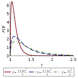
where $G$ is the Mejier $G$-function [11, 12, 13]; Figure 1 reports the above PDF for three different temperatures.

Figure 1: The PDF of the relativistic MB as function of $\gamma$ for different values of T.

The average value or mean, $\mu$, is

$$\mu(T)=\frac{2\,TG^{3,0}_{1,3}\left(\frac{1}{4T^{2}}\,\Big{|}\,^{1}_{-1/2,-1/2,-1}\right)}{G^{3,0}_{1,3}\left(\frac{1}{4T^{2}}\,\Big{|}\,^{1}_{-1/2,-1,-3/2}\right)}\quad,$$ (8)

the second moment about the origin is

$$\mu(T)^{2}=\frac{4\,{T}^{2}G^{3,0}_{1,3}\left(1/4\,{T}^{-2}\,\Big{|}\,^{1}_{0,-1/2,-1/2}\right)}{G^{3,0}_{1,3}\left(1/4\,{T}^{-2}\,\Big{|}\,^{1}_{-1/2,-1,-3/2}\right)}\quad,$$ (9)

the variance, $\sigma^{2}$ is

$$\sigma^{2}(T)=$$

$$\frac{4\,{T}^{2}\left(G^{3,0}_{1,3}\left(\frac{1}{4T^{2}}\,\Big{|}\,^{1}_{-1/2,-1,-3/2}\right)G^{3,0}_{1,3}\left(\frac{1}{4T^{2}}\,\Big{|}\,^{1}_{0,-1/2,-1/2}\right)-\left(G^{3,0}_{1,3}\left(\frac{1}{4T^{2}}\,\Big{|}\,^{1}_{-1/2,-1/2,-1}\right)\right)^{2}\right)}{\left(G^{3,0}_{1,3}\left(\frac{1}{4T^{2}}\,\Big{|}\,^{1}_{-1/2,-1,-3/2}\right)\right)^{2}}\quad.$$ (10)

The mode is the real solution of the following cubic equation in $\gamma$

$${{\it\gamma}}^{3}+3\,T{{\it\gamma}}^{2}-{\it\gamma}-4\,T=0\quad,$$ (11)

which has the real solution

$$mode=\frac{1}{6}\,\sqrt[3]{324\,T-216\,{T}^{3}+12\,\sqrt{-1296\,{T}^{4}+621\,{T}^{2}-12}}$$

$$-6\,{\frac{-1/3-{T}^{2}}{\sqrt[3]{324\,T-216\,{T}^{3}+12\,\sqrt{-1296\,{T}^{4}+621\,{T}^{2}-12}}}}-T\quad.$$ (12)

At the moment of writing a closed form for the distribution function (DF) which is

$$F_{r}(\gamma;T)=\int_{1}^{y}f_{r}(\gamma;T)d\gamma\quad,$$ (13)

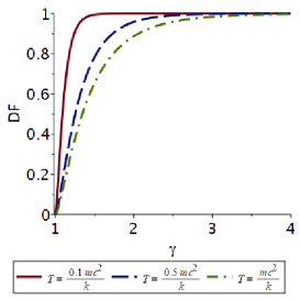
does not exists and we therefore present a numerical integration, see Figure 2.

Figure 2: The numerical DF of the relativistic MB as function of $\gamma$ for different values of T.

The asymptotic behavior of the PDF, $f_{a}$, is

$$f_{a}(\gamma;T)=\frac{1}{G^{3,0}_{1,3}\left(1/4\,{T}^{-2}\,\Big{|}\,^{1}_{-1/2,-1,-3/2}\right)\,2048\,{{\it\gamma}}^{21}}{T}^{3}\Bigg{(}65536\,{{\it\gamma}}^{18}-32768\,{{\it\gamma}}^{16}-8192\,{{\it\gamma}}^{14}$$

$$-4096\,{{\it\gamma}}^{12}-2560\,{{\it\gamma}}^{10}-1792\,{{\it\gamma}}^{8}-1344\,{{\it\gamma}}^{6}-1056\,{{\it\gamma}}^{4}-858\,{{\it\gamma}}^{2}-715\Bigg{)}{{\rm e}^{-{\frac{{\it\gamma}}{T}}}}\quad.$$ (14)

The integration of the above approximate PDF gives an approximate DF which has a maximum percentage error of $7\%$ in the interval $1.1<\gamma<4$ when $T=1$. The random numbers belonging to the relativistic MB can be generated through a numerical computation of the inverse function following the algorithm outlined in Sec. 4.9.1 of [14]. The above PDF has only one parameter which can be derived approximating the average value with a Pade approximant $[2,2]$

$$\mu(T)\approx{\frac{-0.061723842+1.542917977\,T+0.3269078746\,\left(T-1\right)^{2}}{0.1069596119+0.8930403881\,T+0.1511024609\,\left(T-1\right)^{2}}}\quad.$$ (15)

The above approximation in the interval $0.1\leq T<10$ has a percent error less than 1$\%$. The inverse function allows to derive $T$ as

$$T=-\frac{1}{2}\,{\frac{5.908\times 10^{9}\,{\it\bar{x}}-8.89\times 10^{9}+\sqrt{{1.931\times 10^{19}}\,{{\it\bar{x}}}^{2}-{5.528\times 10^{19}}\,{\it\bar{x}}+{4.437\times 10^{19}}}}{1.511\times 10^{9}\,{\it\bar{x}}-3.269\times 10^{9}}}\quad.$$ (16)

Here $\bar{x}$ is the sample mean defined as

$$\bar{x}=\frac{1}{n}\sum_{i=1}^{n}x_{i}\quad,$$ (17)

formula which is useful to derive the variance of the sample

$$Var=\frac{1}{n-1}\sum_{i=1}^{n}(x_{i}-{\bar{x}})^{2}\quad,$$ (18)

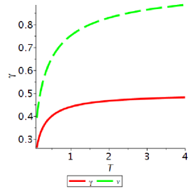
where $x_{i}$ are the n-data, see[15]. An example of random generation of points is reported in Figure 3 where we imposed $T=1$ and we found $T=1.0397$ from the generated random sample.

Figure 3: The DF for 3000 random points generated according to the relativistic MB (blue steps diagram) and the theoretical DF (red dashed line) see 3.

2.2 Variable velocity

We now return to the variable velocity, the PDF is

$$f_{r}(v;T)=\frac{32\,\sqrt{-{\frac{{v}^{2}}{{v}^{2}-1}}}{{\rm e}^{{\frac{\sqrt{-{v}^{2}+1}-1}{\sqrt{-{v}^{2}+1}T}}}}\sqrt{-{v}^{2}+1}{T}^{3}v}{{{\rm e}^{{T}^{-1}}}G^{3,0}_{1,3}\left(1/4\,{T}^{-2}\,\Big{|}\,^{1}_{-1/2,-1,-3/2}\right)}\quad,$$ (19)

where $v$ is expressed in $c=1$ units. The mode is a solution of a sextic equation, see [16], in $v$

$$-4\,{T}^{2}{v}^{6}+12\,{T}^{2}{v}^{4}-{v}^{4}-12\,{T}^{2}{v}^{2}+4\,{T}^{2}=0\quad,$$ (20)

which has the following real solution

$$mode=\frac{1}{6}\,\Bigg{(}3\,{\frac{\sqrt[3]{24\,\sqrt{3}\sqrt{27\,{T}^{2}-1}{T}^{3}-216\,{T}^{4}+36\,{T}^{2}-1}}{{T}^{2}}}$$

$$-3\,{\frac{24\,{T}^{2}-1}{{T}^{2}\sqrt[3]{24\,\sqrt{3}\sqrt{27\,{T}^{2}-1}{T}^{3}-216\,{T}^{4}+36\,{T}^{2}-1}}}+3\,{\frac{12\,{T}^{2}-1}{{T}^{2}}}\Bigg{)}^{1/2}\quad.$$ (21)

The position of the mode for the PDF in $v$ is different from that one in $\gamma$, see Figure 4.

Figure 4: The position of the mode in the two PDFs: gamma variable (red full line) and v variable (dashed green line).

At the moment of writing the other statistical parameters cannot be presented in a closed form.

3 The Maxwell Jüttner distribution

The PDF for the Maxwell Jüttner (MJ) distribution is

$$f_{MJ}(\gamma;\Theta)=\frac{\gamma\,\sqrt{{\gamma}^{2}-1}{{\rm e}^{-{\frac{\gamma}{\Theta}}}}}{\Theta\,{{\sl K}_{2}\left(\frac{1}{\Theta}\right)}}\quad,$$ (22)

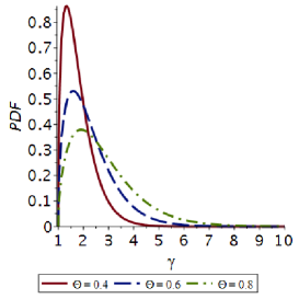
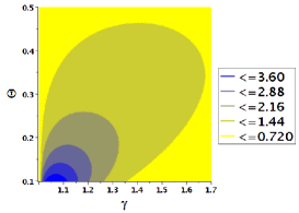
where $\Theta=\sqrt{\frac{kT_{MB}}{m\,c^{2}}}$, $m$ is the mass of the gas molecules, $k$ is the Boltzmann constant, $T_{MB}$ is the usual thermodynamic temperature and ${\sl K}_{2}(x)$ is the Bessel function of second kind, see [3, 4, 6, 7]. Figure 5 reports the above PDF for three different values of $\Theta$ and Figure 6 displays the PDF as a 2-D contour.

Figure 5: The PDF of the MJ as function of $\gamma$ for different values of $\Theta$.

Figure 6: A 2-D contour for the MJ PDF as function of $\gamma$ and $\Theta$.

The average value is

$$\mu(\Theta)=\frac{-2\,{\Theta}^{2}G^{2,1}_{1,3}\left(\frac{1}{4\Theta^{2}}\,\Big{|}\,^{1}_{3/2,-1/2,-2}\right)}{{{\sl K}_{2}\left(\frac{1}{\Theta}\right)}}$$ (23)

and the variance is

$$\sigma^{2}(\Theta)=\frac{1}{{\Theta}^{2}\left({{\sl K}_{2}\left(\frac{1}{\Theta}\right)}\right)^{2}}\Bigg{(}-4\,{\Theta}^{5}\Big{(}2\,{{\sl K}_{1}\left({\Theta}^{-1}\right)}G^{2,1}_{1,3}\left(1/4\,{\Theta}^{-2}\,\Big{|}\,^{1}_{5/2,-1/2,-2}\right)\Theta$$

$$+\left(G^{2,1}_{1,3}\left(1/4\,{\Theta}^{-2}\,\Big{|}\,^{1}_{3/2,-1/2,2}\right)\right)^{2}\Theta+{{\sl K}_{0}\left({\Theta}^{-1}\right)}G^{2,1}_{1,3}\left(1/4\,{\Theta}^{-2}\,\Big{|}\,^{1}_{5/2,-1/2,2}\right)\Big{)}\Bigg{)}\quad.$$ (24)

The mode can be found by solving the following cubic equation

$$\frac{d}{d\,\gamma}f_{MJ}(\gamma;\Theta)\propto-{\gamma}^{3}+2\,\Theta\,{\gamma}^{2}+\gamma-\Theta=0\quad.$$ (25)

The real solution is

$$mode=\frac{1}{6\,\sqrt[3]{-36\,\Theta+64\,{\Theta}^{3}+12\,\sqrt{-96\,{\Theta}^{4}-39\,{\Theta}^{2}-12}}}\times$$

$$\Bigg{(}\left(-36\,\Theta+64\,{\Theta}^{3}+12\,\sqrt{-96\,{\Theta}^{4}-39\,{\Theta}^{2}-12}\right)^{{\frac{2}{3}}}$$

$$+4\,\Theta\,\sqrt[3]{-36\,\Theta+64\,{\Theta}^{3}+12\,\sqrt{-96\,{\Theta}^{4}-39\,{\Theta}^{2}-12}}+16\,{\Theta}^{2}+12\Bigg{)}\quad.$$ (26)

The asymptotic expansion of order 10 for the PDF is

$$f_{MJ}(\gamma;\Theta)\sim\frac{1}{\Theta\,{{\sl K}_{2}\left(\frac{1}{\Theta}\right)}}\frac{\left(128\,{\gamma}^{8}-64\,{\gamma}^{6}-16\,{\gamma}^{4}-8\,{\gamma}^{2}-5\right){{\rm e}^{-{\frac{\gamma}{\Theta}}}}}{128\,{\gamma}^{6}}\quad.$$ (27)

The DF is evaluated with the following integral

$$F_{MJ}(\gamma;\Theta)=\int_{1}^{\gamma}f_{MJ}(\gamma;\Theta)\,d\gamma\quad,$$ (28)

which cannot be expressed in terms of special functions.

We now present some approximations for the distribution function A first approximation is given by a series expansion when, ad example , $\Theta=1$

$$F_{MJ}(\gamma;1)=\frac{1}{{\sl K}_{2}(1)}\Bigg{(}{{\sl K}_{2}\left(1\right)}+\sqrt{\pi}\sum_{m=0}^{\infty}{\frac{\left(-1\right)^{1+m}\Gamma\left(3-2\,m,\gamma\right)}{\Gamma\left(1+m\right)\Gamma\left({\frac{3}{2}}-m\right)}}\Bigg{)}\quad,$$ (29)

which has a percent error less $<0.6\%$ in interval $1.1<\gamma<10$ when $T=1$. A second approximation is given by an asymptotic expansion of order 50 for the PDF followed by the integration, see Figure 7.

Figure 7: The numerical MJ DF as function of $\gamma$ for different values of $\Theta$.

The parameter $\Theta$ can be derived from the experimental sample once the average value is modeled by a Pade approximant $[2,2]$ and the inverse function is derived

$$\Theta=0.1661\,{\it\bar{x}}-0.3085+1.36051\times 10^{-10}\,\sqrt{1.4908\times 10^{18}\,{{\it\bar{x}}}^{2}+5.913\times 10^{18}\,{\it\bar{x}}-6.5835\times 10^{18}}\quad.$$ (30)

An analogous formula allows to derive $\Theta$ from the variance $Var$ of the sample

$$\Theta=\frac{1}{4}\times$$

$${\frac{1.818\times 10^{10}{\it Var}+5.972\times 10^{11}+5\sqrt{{2.277\times 10^{20}}{{\it Var}}^{2}+{7.814\times 10^{23}}{\it Var}-{3.597\times 10^{22}}}}{5.436\times 10^{8}{\it Var}+1.978\times 10^{12}}}\quad.$$ (31)

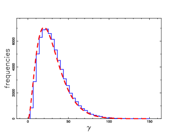
An example of random generation of points is reported in Figure 8 where we imposed $T=10$ and we found $T=9.97$ from formula (30) and $T=9.98$ from formula (31).

Figure 8: The PDF for 70000 random points generated according to the MJ (blue steps) and the theoretical PDF (red dashed line), see formula (22).

3.1 Variable $\beta$

We now change the variable of integration $\gamma$ in $\beta=\frac{v}{c}$, the PDF of the MJ is

$$f_{MJ}(\beta;\Theta)=\frac{\sqrt{\left(1-{\beta}^{2}\right)^{-1}-1}{{\rm e}^{-{\frac{1}{\Theta}{\frac{1}{\sqrt{1-{\beta}^{2}}}}}}}\beta}{\left({1-\beta}^{2}\right)^{2}\Theta\,{{\sl K}_{2}\left(\frac{1}{\Theta}\right)}}\quad,$$ (32)

where $0\leq\beta\leq 1$, see Figure 9.

Figure 9: The 3D surface of the MJ PDF as function of $\Theta$ and $\beta$.

We have only one analytical result, the mode, which is found solving the following equation in $\beta$

$$-3\,\left(\beta-1\right)^{3}\left(\beta+1\right)^{3}\left(\Theta\,\left({\beta}^{2}+2/3\right)\sqrt{-{\beta}^{2}+1}-1/3\,{\beta}^{2}\right){{\rm e}^{-{\frac{1}{\sqrt{-{\beta}^{2}+1}\Theta}}}}{\beta}^{2}=0\quad.$$ (33)

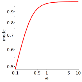
As an example when $\Theta=0.1$ the mode is at $\beta=0.4866$ and Figure 10 reports the mode as function of $\Theta$.

Figure 10: The mode of the MJ distribution for different values of $\Theta$.

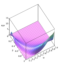
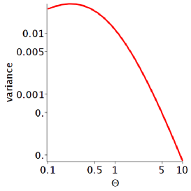
The mean and the variance of the MJ distribution does not have an analytical expression and they are reported in a numerical way, see Figures 11 and 12.

Figure 11: The mean of the MJ distribution for different values of $\Theta$.

Figure 12: The variance of the MJ distribution for different values of $\Theta$.

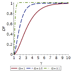
The DF of the MJ is given by the following integral

$$F_{MJ}(\beta;\Theta)=\int_{0}^{\beta}f_{MJ}(\beta;\Theta)\,d\beta\quad,$$ (34)

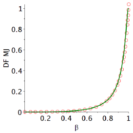
with $\beta$ in [0,1] which does not have an analytical expression. An approximation is given by the Riemann sums, see [17], when $\Theta=1$

$$F_{MJ}(\beta;\Theta)=$$

$$\frac{\beta\sum_{{\it i}=0}^{9}{\frac{\beta}{10\,{{\sl K}_{2}\left(1\right)}}\sqrt{\left(-{\frac{{\beta}^{2}}{100}\left({\it i}+{\frac{1}{2}}\right)^{2}}+1\right)^{-1}-1}{{\rm e}^{-{\frac{1}{\sqrt{-{\frac{{\beta}^{2}}{100}\left({\it i}+{\frac{1}{2}}\right)^{2}}+1}}}}}\left({\it i}+{\frac{1}{2}}\right)\left(-{\frac{{\beta}^{2}}{100}\left({\it i}+{\frac{1}{2}}\right)^{2}}+1\right)^{-2}}}{10}\quad,$$ (35)

see Figure 13. The above DF has a maximum percentage error of $\approx 10\%$ at $\beta=1$.

Figure 13: The numerical DF of the MJ distribution (red circles) and the Riemann approximation (green line) as function of $\beta$.

4 The astrophysical applications

This section reviews the synchrotron emissivity for a single relativistic electron, derives the spectral synchrotron emissivity for the two relativistic distributions here analyzed and models the observed synchrotron emission in some astrophysical sources.

4.1 Synchrotron emissivity

The synchrotron emissivity of a single electron is

$$\frac{\sqrt{3}e^{3}B\sin(\alpha)}{8\pi^{2}\epsilon_{0}cm_{e}}F(x)\quad,$$ (36)

where, according to eqn.(8.58) in [18], $e$ is the electron charge, $B$ is the magnetic field, $\alpha$ is the pitch angle, $\epsilon_{0}$ is the permittivity of free space, $c$ is the light velocity, $m_{e}$ is the electron mass, $x=$ is the ratio of the angular frequency ($\omega$) to the critical angular frequency ($\omega_{c}$) and

$$F(x)=x\int_{x}^{\infty}K_{5/3}(z)dz$$ (37)

where $K_{5/3}(z)$ is the modified Bessel function of second kind with order 5/3 [19, 13]. The modified Bessel function is also known as Basset function, modified Bessel function of the third kind or Macdonald function see pag. 527 in [20]. The above function has the following analytical expression

$$F(x)=-{\frac{9\,\sqrt{3}\sqrt[3]{2}\pi}{320\,\Gamma\left(2/3\right)}{x}^{{\frac{11}{3}}}{\mbox{${}_{1}$F${}_{2}$}({\frac{4}{3}};\,{\frac{7}{3}},{\frac{8}{3}};\,{\frac{{x}^{2}}{4}})}}-{\frac{x\sqrt{3}\pi}{3}}+\sqrt[3]{x}{2}^{{\frac{2}{3}}}\Gamma\left({\frac{2}{3}}\right){\mbox{${}_{1}$F${}_{2}$}(-{\frac{1}{3}};\,-{\frac{2}{3}},{\frac{2}{3}};\,{\frac{{x}^{2}}{4}})}\quad,$$ (38)

where ${\leavevmode\nobreak\ {}_{2}F_{1}(a,b;\,c;\,v)}$ is a regularized hypergeometric function [19, 21, 22, 13]. Figure 14 displays $F(x)$ as function of $x$.

Figure 14: F(x) as function of $x$ with logarithmic axes.

4.2 The synchrotron relativistic MB distribution

We start from the PDF for the relativistic MB distribution as represented by equation (7) and we perform the following first change of variable

$$\gamma=\frac{E}{m_{e}c^{2}}\quad,$$ (39)

where $E$ is the relativistic energy. The resulting PDF in relativistic energy is

$$f_{r}(E;T)=\frac{32\,\sqrt{{\frac{{E}^{2}}{{m_{{e}}}^{2}{c}^{4}}}-1}{{\rm e}^{{\frac{1}{T}\left(1-{\frac{E}{m_{{e}}{c}^{2}}}\right)}}}{T}^{3}{m_{{e}}}^{3}{c}^{6}}{{E}^{4}{{\rm e}^{{T}^{-1}}}G^{3,0}_{1,3}\left({\frac{1}{4\,{T}^{2}}}\,\Big{|}\,^{1}_{-{\frac{1}{2}},-1,-{\frac{3}{2}}}\right)}\quad.$$ (40)

A second change of variable is

$$E=\sqrt{{\frac{\nu}{\nu_{{g}}}}}m_{{e}}{c}^{2}\quad,$$ (41)

produces

$$f_{r}(\nu;T,\nu_{{g}})=\frac{16\,\sqrt{{\frac{\nu}{\nu_{{g}}}}-1}{{\rm e}^{{\frac{1}{T}\left(1-\sqrt{{\frac{\nu}{\nu_{{g}}}}}\right)}}}{T}^{3}\nu_{{g}}}{{\nu}^{2}{{\rm e}^{{T}^{-1}}}G^{3,0}_{1,3}\left({\frac{1}{4\,{T}^{2}}}\,\Big{|}\,^{1}_{-{\frac{1}{2}},-1,-{\frac{3}{2}}}\right)\sqrt{{\frac{\nu}{\nu_{{g}}}}}}\quad,$$ (42)

where

$$\nu_{g}=\frac{eB}{2\pi m_{e}}\quad.$$ (43)

We know that $\nu_{g}=2.799249\,10^{12}\,B$ where $B$ is the magnetic field expressed in gauss and therefore the above PDF in frequency becomes

$$f_{r}(\nu;T,B)=\frac{{7.49345\times 10^{19}}\,\sqrt{{3.57238\times 10^{-13}}\,{\frac{\nu}{B}}-1}{{\rm e}^{{\frac{1}{T}\left(1-5.97694\times 10^{-7}\,\sqrt{{\frac{\nu}{B}}}\right)}}}{T}^{3}B}{{\nu}^{2}{{\rm e}^{{T}^{-1}}}G^{3,0}_{1,3}\left({\frac{1}{4\,{T}^{2}}}\,\Big{|}\,^{1}_{-{\frac{1}{2}},-1,-{\frac{3}{2}}}\right)\sqrt{{\frac{\nu}{B}}}}\quad.$$ (44)

4.3 The synchrotron Maxwell Jüttner distribution

We start from the PDF for the Maxwell Jüttner distribution as given by equation (22) and we perform two changes in variable as in the previous section. The resulting PDF in relativistic energy is

$$f_{MJ}(E;\Theta)=\frac{E\sqrt{{\frac{{E}^{2}}{{m_{{e}}}^{2}{c}^{4}}}-1}{{\rm e}^{-{\frac{E}{m_{{e}}{c}^{2}\Theta}}}}}{{m_{{e}}}^{2}{c}^{4}\Theta\,{{\sl K}_{2}\left(\frac{1}{\Theta}\right)}}\quad.$$ (45)

The second PDF in $\nu$ is

$$f_{MJ}(\nu;\Theta,\nu_{{g}})=\frac{\sqrt{{\frac{\nu}{\nu_{{g}}}}-1}{{\rm e}^{-{\frac{1}{\Theta}\sqrt{{\frac{\nu}{\nu_{{g}}}}}}}}}{2\,\Theta\,{{\sl K}_{2}\left(\frac{1}{\Theta}\right)}\nu_{{g}}}\quad.$$ (46)

The astrophysical PDF in frequency for the Maxwell Jüttner distribution is

$$f_{MJ}(\nu;\Theta,B)=\frac{{1.78619\times 10^{-13}}\,\sqrt{{3.57238\times 10^{-13}}\,{\frac{\nu}{B}}-1}{{\rm e}^{-5.97694\times 10^{-7}\,{\frac{1}{\Theta}\sqrt{{\frac{\nu}{B}}}}}}}{\Theta\,{{\sl K}_{2}\left(\frac{1}{\Theta}\right)}B}\quad.$$ (47)

The mismatch between measured flux in Jy and theoretical flux, $S_{theo}$, can be obtained introducing a multiplicative constant $C$

$$S_{theo}=C\times f_{MJ}(\nu;\Theta,B)\quad.$$ (48)

4.4 The spectrum of the radio-sources

As a first example we analyze the spectrum of an extended region around M87, see as example Figure 1 in [23] where the flux in Jy as function of the frequency is reported in the range $9\times 10^{9}\,Hz<\nu<2\times 10^{18}\,Hz$. Figure 15 reports the measured and theoretical flux in the range $9\times 10^{9}\,Hz<\nu<2\times 10^{12}\,Hz$ for the quiet core of M87.

Figure 15: Measured flux in Jy (green stars) of the quiet core of M87 and the theoretical flux (red line) for the Maxwell Jüttner distribution as given by equation (48). The numerical parameters are $B=10^{-5}\,gauss$, $\Theta=30$ and $C=10^{12}\,Jy$.

A second example is given by the radio sources with ultra steep spectra (USS) which are characterized by a spectral index, $\alpha$, lower than -1.30 when the radio flux, $S$, is proportional to $S^{\alpha}$, see [24]. As a practical example we select the cluster Abell 1914 where the measured total flux densities at 150 MHz and 1.4 GHz are $S_{150}=4.68\,$Jy and $S_{1.4}$ = 34.8 mJy which means $\alpha=-2.17$. We now evaluate the theoretical spectral index of synchrotron emission for the relativistic MB distribution between 150 MHz and 1.4 GHz when $B$ is fixed and $T$ variable, see Figure 16

Figure 16: The spectral index of the relativistic MB as function of $T$ when $B=1.0\times 10^{-6}$.

and Figure 17 when $T$ and $B$ are both variables.

Figure 17: The spectral index of the relativistic MB as function of $T$ and $B$ in gauss.

The two Figures above show that the theoretical spectral index is always smaller than -2 which can be considered as an asymptotic limit for high values of relativistic temperature. As an example when $B=1.0\times 10^{-5}gauss$ the spectral index is -2.17 when $T=10$.

5 Conclusions

The relativistic MB distribution has been derived in [10] without any particular statistics: here we derived, when the main variable is the Lorentz factor $\gamma$, the constant of normalization, the average value, the second moment about the origin, the variance, the mode, the asymptotic behavior, an approximate expression for the average value as function of the temperature and an inverted expression for the temperature as function of average value.

We derived the following statistical parameters of the MJ distribution when $\gamma$ is the main variable: average value, variance, mode, asymptotic expansion, two approximate expressions for the distribution function, a first evaluation of $\Theta$ from the average value and a second evaluation of $\Theta$ from the variance.

Following the usual argument which suggests a power law behavior for the spectral distribution of the synchrotron emission in presence of a power law distribution for the energy of the electrons we derived the spectral distribution for the relativistic MB and MJ distributions which are now function of the selected generalized temperature and the magnetic field. Two astrophysical applications are given: the spectral distribution of emission in the core of M87 in the framework of the synchrotron emissivity and an explanation for the steep spectra sources in the framework of the synchrotron emissivity for the relativistic MJ distribution.

References

- [1] Maxwell J C 1860 V. illustrations of the dynamical theory of gases.—part i. on the motions and collisions of perfectly elastic spheres The London, Edinburgh, and Dublin Philosophical Magazine and Journal of Science 19(124), 19
- [2] Boltzmann L 1872 Weitere studien über das wärmegleichgewicht unter gasmolekülen K. Acad. Wiss.(Wein) Sitzb., II Abt 66, 275
- [3] Jüttner F 1911 Das maxwellsche gesetz der geschwindigkeitsverteilung in der relativtheorie Annalen der Physik 339(5), 856
- [4] Synge J 1957 The relativistic gas (New York: North-Holland)
- [5] Aragón-Muñoz L and Chacón-Acosta G 2018 Modified relativistic jüttner-like distribution functions with -parameter in J. Phys. Conf. Ser vol 1030 p 012004
- [6] Livadiotis G 2016 Modeling anisotropic maxwell-jüttner distributions: derivation and properties in Annales Geophysicae (Copernicus GmbH) vol 34 p 1145
- [7] Tsouros A and Kylafis N D 2017 The energy distribution of electrons in radio jets A&A 603 L4 (Preprint 1706.05227)
- [8] Sadegzadeh S and Mousavi A 2018 Maxwell-Jüttner distributed counterstreaming magnetoplasmas—Parallel propagation Physics of Plasmas 25(11) 112107
- [9] Freund J 2008 Special Relativity for Beginners: a Textbook for Undergraduates (Singapore: World Scientific Press)
- [10] Claycomb J 2018 Mathematical Methods for Physics: Using MATLAB and Maple (Boston: Mercury Learning & Information)
- [11] Meijer C 1936 Uber Whittakersche bzw. Besselsche Funktionen und deren Produkte. Nieuw Arch. Wiskd. 18, 10
- [12] Meijer C 1941 Multiplikationstheoreme fur die Funktion . Proc. Akad. Wet. Amsterdam 44, 1062
- [13] Olver F W J, Lozier D W, Boisvert R F and Clark C W 2010 NIST Handbook of Mathematical Functions (Cambridge: Cambridge University Press. )
- [14] Brandt S and Gowan G 1998 Data Analysis: Statistical and Computational Methods for Scientists and Engineers (New-York: Springer & Verlag)
- [15] Press W H, Teukolsky S A, Vetterling W T and Flannery B P 1992 Numerical Recipes in FORTRAN. The Art of Scientific Computing (Cambridge, UK: Cambridge University Press)
- [16] Hagedorn T R 2000 General formulas for solving solvable sextic equations Journal of Algebra 233(2), 704
- [17] Anton H, Bivens I and Davis S 2012 Calculus, 10th Edition (New York: Wiley) ISBN 9781118404003
- [18] Longair M S 2011 High Energy Astrophysics III ed. (Cambridge: Cambridge University Press)
- [19] Abramowitz M and Stegun I A 1965 Handbook of Mathematical Functions with Formulas, Graphs, and Mathematical Tables (New York: Dover)
- [20] Oldham K B, Myland J and Spanier J 2010 An atlas of functions: with equator, the atlas function calculator (New York: Springer Science & Business Media)
- [21] von Seggern D 1992 CRC Standard Curves and Surfaces (New York: CRC)
- [22] Thompson W J 1997 Atlas for computing mathematical functions (New York: Wiley-Interscience)
- [23] Prieto M A, Fernández-Ontiveros J A, Markoff S, Espada D and González-Martín O 2016 The central parsecs of M87: jet emission and an elusive accretion disc MNRAS 457(4), 3801 (Preprint 1508.02302)
- [24] De Breuck C, van Breugel W, Röttgering H J A and Miley G 2000 A sample of 669 ultra steep spectrum radio sources to find high redshift radio galaxies A&AS 143, 303 (Preprint astro-ph/0002297)