Stochastic Damped L-BFGS with Controlled Norm of the Hessian Approximation

Abstract

We propose a new stochastic variance-reduced damped L-BFGS algorithm, where we leverage estimates of bounds on the largest and smallest eigenvalues of the Hessian approximation to balance its quality and conditioning. Our algorithm, VARCHEN, draws from previous work that proposed a novel stochastic damped L-BFGS algorithm called SdLBFGS. We establish almost sure convergence to a stationary point and a complexity bound. We empirically demonstrate that VARCHEN is more robust than SdLBFGS-VR and SVRG on a modified DavidNet problem—a highly nonconvex and ill-conditioned problem that arises in the context of deep learning, and their performance is comparable on a logistic regression problem and a nonconvex support-vector machine problem.

1 Introduction and Related Work

We consider unconstrained stochastic minimization problems of $f:\mathbb{R}^{n}\to\mathbb{R}$ where

$$f(x)=\mathbb{E}_{\xi}[F(x,\xi)]\ \text{(online)}\quad\text{or}\quad f(x)=\frac{1}{N}\sum_{i=1}^{N}f_{i}(x)\ \text{(finite sum)},$$ (1)

where $\xi\in\mathbb{R}^{d}$ denotes a random variable, $F:\mathbb{R}^{n}\times\mathbb{R}^{d}\to\mathbb{R}$ is continuously differentiable and possibly nonconvex, $f_{i}$ is the loss corresponding to the $i$-th element of our dataset and $N$ is the size of the dataset. The algorithm developed below applies to both online and finite-sum problems.

Stochastic Gradient Descent (SGD) (Robbins and Monro, 1951; Bottou, 2010) and its variants (Polyak, 1964; Nesterov, 1983; Duchi et al., 2011; Tieleman and Hinton, 2012; Kingma and Ba, 2015), including variance-reduced algorithms (Johnson and Zhang, 2013; Nguyen et al., 2017; Fang et al., 2018; Wang et al., 2019), are widely used to solve (1) in machine learning. However, they might not be well-suited for highly nonconvex and ill-conditioned problems (Bottou et al., 2018), which are more effectively treated using (approximate) second-order information. Second-order algorithms are well studied in the deterministic case (Dennis and Moré, 1974; Dembo et al., 1982; Dennis Jr and Schnabel, 1996; Amari, 1998) but there are many areas to explore in the stochastic context that go beyond existing works (Schraudolph et al., 2007; Bordes et al., 2009; Byrd et al., 2016; Moritz et al., 2016; Gower et al., 2016). Among these areas, the use of damping in L-BFGS is an interesting research direction to be leveraged in the stochastic case. Wang et al. (2017) proposed a stochastic damped L-BFGS (SdLBFGS) algorithm and proved almost sure convergence to a stationary point. However, damping does not prevent the inverse Hessian approximation $H_{k}$ from being ill-conditioned (Chen et al., 2019). The convergence of SdLBFGS may be heavily affected if the Hessian approximation becomes nearly singular during the iterations. In order to remedy this issue, Chen et al. (2019) proposed to combine SdLBFGS with regularized BFGS Mokhtari and Ribeiro (2014). Our approach differs.

Our contributions:

• Less restrictive assumptions: we force $H_{k}$ to be uniformly bounded and positive definite by requiring the stochastic gradient to be Lipschitz continuous, which is a less restrictive assumption than those of Wang et al. (2017), who require the stochastic function to be twice differentiable with respect to the parameter vector, and its Hessian to be bounded for all parameter and random sampling vectors.

• A new damped L-BFGS: we propose a new version of stochastic damped L-BFGS that maintains estimates of the smallest and largest eigenvalues of $H_{k}$. A solution is proposed when ill-conditioning is detected that preserves almost sure convergence to a stationary point.

• Choice of the initial inverse Hessian approximation: we propose a new formula for the initial inverse Hessian approximation to make the algorithm more robust to ill-conditioning.

Notation

For a symmetric matrix $A$, we use $A\succ 0$ to indicate that $A$ is positive definite, and $\lambda_{\min}(A)$ and $\lambda_{\max}(A)$ to denote its smallest and largest eigenvalue, respectively. If $B$ is also symmetric, $B\preceq A$ means that $A-B$ is positive semidefinite. The identity matrix of appropriate size is denoted $I$. Finally, $\mathbb{E}_{\xi}[.]$ is the expectation over random variable $\xi$.

2 Formulation of our method

We assume that at iteration $k$, we can obtain a stochastic approximation

$$g(x_{k},\xi_{k})=\frac{1}{m_{k}}\sum_{i=1}^{m_{k}}\nabla f_{\xi_{k,i}}(x_{k})$$ (2)

of $\nabla f(x_{k})$, where $\xi_{k}$ denotes the subset of samples taken from a given set of realizations of $\xi$. The Hessian approximation constructed at iteration $k$ and its inverse are denoted by $B_{k}$ and $H_{k}$, respectively, such that $H_{k}=B_{k}^{-1}$ and $B_{k}\succ 0$. Iterates are updated according to

$$x_{k+1}=x_{k}+\alpha_{k}d_{k},\quad\text{where}\quad d_{k}=-H_{k}g(x_{k},\xi_{k})\quad\text{and}\quad\alpha_{k}>0\,\text{is the step size.}$$ (3)

The stochastic BFGS method (Schraudolph et al., 2007) computes an updated approximation $H_{k+1}$ according to

$$H_{k+1}=V_{k}H_{k}V_{k}^{\top}+\rho_{k}s_{k}s_{k}^{\top},\quad\text{where }\quad V_{k}=I-\rho_{k}s_{k}y_{k}^{\top}\quad\text{and}\quad\rho_{k}=1/s_{k}^{\top}y_{k},$$ (4)

which ensures that the secant equation $B_{k+1}s_{k}=y_{k}$ is satisfied, where

$$s_{k}=x_{k+1}-x_{k},\quad\text{and}\quad y_{k}=g(x_{k+1},\xi_{k})-g(x_{k},\xi_{k}).$$ (5)

If $H_{k}\succ 0$ and the curvature condition $s_{k}^{\top}y_{k}>0$ holds, then $H_{k+1}\succ 0$ (see, for instance, Fletcher, 1970).

Because storing $H_{k}$ and performing matrix-vector products is costly for large-scale problems, we use the limited-memory version of BFGS (L-BFGS) (Nocedal, 1980; Liu and Nocedal, 1989), in which $H_{k}$ only depends on the most recent $p$ iterations and an initial $H_{k}^{0}\succ 0$. The parameter $p$ is the memory of L-BFGS. The inverse Hessian update can be written as

$$H_{k}= \ (V_{k-1}^{\top}\dots V_{k-p}^{\top})H_{k}^{0}(V_{k-p}\dots V_{k-1})+$$ (6)

$$\rho_{k-p}(V_{k-1}^{\top}\dots V_{k-p+1}^{\top})s_{k-p}s_{k-p}^{\top}(V_{k-p+1}\dots V_{k-1})+\dots+\rho_{k-1}s_{k-1}s_{k-1}^{\top}.$$

When $\alpha_{k}$ in (3) is not computed using a Wolfe line search (Wolfe, 1969, 1971), there is no guarantee that the curvature condition holds. A common strategy is to simply skip the update. By contrast, Powell (1978) proposed damping, which consists in updating $H_{k}$ using a modified $y_{k}$, denoted by $\hat{y}_{k}$, to benefit from information discovered at iteration $k$ while ensuring sufficient positive definiteness. We use

$$\hat{y}_{k}:=\theta_{k}y_{k}+(1-\theta_{k})B_{k+1}^{0}s_{k},$$ (7)

which is inspired by (Wang et al., 2017), and differs from the original proposal of Powell (1978), where

$$\theta_{k}=1\ \text{ if }\ s_{k}^{\top}y_{k}\geq\eta s_{k}^{\top}B_{k+1}^{0}s_{k},\ \text{ and }\ (1-\eta)\frac{s_{k}^{\top}B_{k+1}^{0}s_{k}}{s_{k}^{\top}B_{k+1}^{0}s_{k}-s_{k}^{\top}y_{k}}\text{ otherwise,}$$ (8)

with $\eta\in(0,1)$ and $B_{k+1}^{0}:=(H_{k+1}^{0})^{-1}$. The choice (7) ensures that the curvature condition

$$s_{k}^{\top}\hat{y}_{k}\geq\eta s_{k}^{\top}B_{k+1}^{0}s_{k}\geq\eta\lambda_{\min}(B_{k+1}^{0})\|s_{k}\|^{2}>0,$$ (9)

is always satisfied since $H_{k+1}^{0}\succ 0$. We obtain the damped L-BFGS update, which is (6) with each $V_{i}$ and $\rho_{i}$ replaced with $\hat{V}_{i}=I-\hat{\rho}_{i}s_{i}^{\top}\hat{y}_{i}$ and $\hat{\rho}_{i}=1/s_{i}^{\top}\hat{y}_{i}$.

3 A new stochastic damped L-BFGS with controlled Hessian norm

Our working assumption is

Assumption 1

There is $\kappa_{\text{low}}\in\mathbb{R}$ such that $f(x)\geq\kappa_{\text{low}}$ for all $x\in\mathbb{R}^{n}$, $f$ is $\mathcal{C}^{1}$ over $\mathbb{R}^{n}$, and there is $L>0$ such that for all $x$, $y\in\mathbb{R}^{n}$, $\|\nabla f(x)-\nabla f(y)\|\leq L\,\|x-y\|$.

We begin by deriving bounds on the smallest and largest eigenvalues of $H_{k+1}$ as functions of bounds on those of $H_{k}$. Proofs can be found in Appendix A.

Lemma 3.1.

Let $s$ and $y\in\mathbb{R}^{n}$ such that $s^{\top}y\geq\gamma\|s\|^{2}$ with $\gamma>0$, and such that $\|y\|\leq L_{y}\|s\|$, with $L_{y}>0$. Let $A=\mu VV^{\top}+\rho ss^{\top}$, where $\rho=1/s^{\top}y$, $\mu>0$, and $V=I-\rho sy^{\top}$. Then,

$$0<\min\left(\frac{1}{L_{y}},\frac{\mu}{1+\frac{\mu}{\gamma}L_{y}^{2}}\right)\leq\lambda_{\min}(A)\leq\lambda_{\max}(A)\leq\frac{1}{\gamma}+\max\left(0,\frac{\mu}{\gamma^{2}}L_{y}^{2}-\frac{\mu}{1+\frac{\mu}{\gamma}L_{y}^{2}}\right).$$

To use Lemma 3.1 to obtain bounds on the eigenvalues of $H_{k+1}$, we make the following assumption:

Assumption 2

There is $L_{g}>0$ such that for all $x$, $y\in\mathbb{R}^{n}$, $\|g(x,\xi)-g(y,\xi)\|\leq L_{g}\,\|x-y\|$.

Assumption 2 is required to prove convergence and convergence rates for most recent stochastic quasi-Newton methods (Yousefian et al., 2017). It is less restrictive than requiring $f(x,\xi)$ to be twice differentiable with respect to $x$, and the Hessian $\nabla_{xx}^{2}f(x,\xi)$ to be bounded for any $x$, $\xi$, as in (Wang et al., 2017).

The next theorem shows that the eigenvalues of $H_{k+1}$ are bounded and bounded away from zero.

Theorem 3.2.

Let Assumptions 1 and 2 hold. Let $H_{k+1}^{0}\succ 0$ and $p>0$. If $H_{k+1}$ is obtained by applying $p$ times the damped BFGS update formula with inexact gradient to $H_{k+1}^{0}$, there exist easily computable constants $\lambda_{k+1}$ and $\Lambda_{k+1}$ that depend on $L_{g}$ and $H_{k+1}^{0}$ such that $0<\lambda_{k+1}\leq\lambda_{\min}(H_{k+1})\leq\lambda_{\max}(H_{k+1})\leq\Lambda_{k+1}$.

The precise form of $\lambda_{k+1}$ and $\Lambda_{k+1}$ is given in Appendix A.

A common choice for $H_{k+1}^{0}$ is $H_{k+1}^{0}=\gamma_{k+1}^{-1}I$ where $\gamma_{k+1}=y_{k}^{\top}y_{k}/s_{k}^{\top}y_{k}$, is the scaling parameter. This choice ensures that the search direction is well scaled, which promotes large steps. To keep $H_{k+1}^{0}$ from becoming nearly singular or non positive definite, we define

$$H_{k+1}^{0}=\left(\max(\underline{\gamma}_{k+1},\min(\gamma_{k+1},\overline{\gamma}_{k+1}))\right)I,$$ (10)

where $0<\underline{\gamma}_{k+1}<\overline{\gamma}_{k+1}$ can be constants or iteration dependent.

The Hessian-gradient product used to compute the search direction $d_{k}=-H_{k}g(x_{k},\xi_{k})$ can be obtained cheaply by exploiting a recursive algorithm (Nocedal, 1980), as described in Algorithm 2 in Appendix B.

Motivated by the success of recent methods combining variance reduction with stochastic L-BFGS (Gower et al., 2016; Moritz et al., 2016; Wang et al., 2017), we apply an SVRG-like type of variance reduction (Johnson and Zhang, 2013) to the update. Not only would this accelerate the convergence, since we can choose a constant step size, but it also improves the quality of the curvature approximation.

We summarize our complete algorithm, VAriance-Reduced stochastic damped L-BFGS with Controlled HEssian Norm (VARCHEN), as Algorithm 1.

Algorithm 1 Variance-Reduced Stochastic Damped L-BFGS with Controlled Hessian Norm

1:  Choose $x_{0}\in\mathbb{R}^{n}$, step size sequence $\{\alpha_{k}>0\}_{k\geq 0}$, batch size sequence $\{m_{k}>0\}_{k\geq 0}$, eigenvalue limits $\lambda_{\max}>\lambda_{\min}>0$, memory parameter $p$, total number of epochs $N_{\text{epochs}}$, and sequences $\{\underline{\gamma}_{k}>0\}_{k\geq 0}$ and $\{\overline{\gamma}_{k+1}>0\}_{k\geq 0}$, such that $0<\lambda_{\min}<\underline{\gamma}_{k}<\overline{\gamma}_{k}<\lambda_{\max}$, for every $k\geq 0$. Set $k=0$ and $H_{0}=I$.

2:  for $t=1,\ldots,N_{\text{epochs}}$ do

3:     Define $x_{k}^{t}=x_{k}$ and compute the full gradient $\nabla f(x_{k}^{t})$. Set $M=0$.

4:     while $M<N$ do

5:        Sample batch $\xi_{k}$ of size $m_{k}\leq N-M$ and compute $g(x_{k},\xi_{k})$ and $g(x_{k}^{t},\xi_{k})$.

6:        Define $\tilde{g}(x_{k},\xi_{k})=g(x_{k},\xi_{k})-g(x_{k}^{t},\xi_{k})+\nabla f(x_{k}^{t})$.

7:        Estimate $\Lambda_{k}$ and $\lambda_{k}$ in Theorem 3.2. If $\Lambda_{k}>\lambda_{\max}$ or $\lambda_{k}<\lambda_{\min}$, delete $s_{i}$, $y_{i}$ and $\hat{y}_{i}$ for $i=k-p+1,\ldots,k-2$.

8:        Compute $d_{k}=-H_{k}\tilde{g}(x_{k},\xi_{k})$.

9:        Define $x_{k+1}=x_{k}+\alpha_{k}d_{k}$, and compute $s_{k}$, $y_{k}$ as in (5), and $\hat{y}_{k}$ as in (7).

10:        Increment $k$ by one and update $M\leftarrow M+m_{k}$.

In step 7 of Algorithm 1, we compute an estimate of the upper and lower bounds on $\lambda_{\max}(H_{k})$ and $\lambda_{\min}(H_{k})$, respectively. The only unknown quantity in the expressions of $\Lambda_{k}$ and $\lambda_{k}$ in Theorem 3.2 is $L_{g}$, which we estimate as $L_{g}\approx L_{g,k}:=\|y_{k}\|/\|s_{k}\|$. When the estimates are not within the limits $[\lambda_{\min},\,\lambda_{\max}]$, we delete $s_{i}$, $y_{i}$ and $\hat{y}_{i}$, $i\in\{k-p+1,\ldots,k-2\}$ from storage, such that $H_{k}g(x_{k},\xi_{k})$ is computed using the most recent pair $(s_{k-1},\hat{y}_{k-1})$ only and $d_{k}=-H_{k}g(x_{k},\xi_{k})$. Finally, a full gradient is computed once in every epoch in step 3. The term $g(x_{k}^{t},\xi_{k})-\nabla f(x_{k}^{t})$ can be seen as the bias in the gradient estimation $g(x_{k},\xi_{k})$, and it is used here to correct the gradient approximation in step 6.

4 Convergence and Complexity Analysis

We show that Algorithm 1 satisfies the assumptions of the convergence analysis and iteration complexity of Wang et al. (2017) for stochastic quasi-Newton methods. We make an additional assumption used by Wang et al. (2017) to establish global convergence.

Assumption 3

For all $k$, $\xi_{k}$ is independent of $\{x_{1},\ldots,x_{k}\}$, $\mathbb{E}_{\xi_{k}}\left[g(x_{k},\xi_{k})\right]=\nabla f(x_{k})$, and there exists $\sigma>0$ such that $\mathbb{E}_{\xi_{k}}[\|g(x_{k},\xi_{k})-\nabla f(x_{k})\|^{2}]\leq\sigma^{2}$.

Our first result follows from Wang et al. (2017, Theorem $2.6$), whose remaining assumptions are satisfied as a consequence of (2), Theorem 3.2, the mechanism of Algorithm 1, (4) and our choice of $\alpha_{k}$ below.

Theorem 4.1.

Assume $m_{k}=m$ for all $k$, that Assumptions 1, 2 and 3 hold for $\{x_{k}\}$ generated by Algorithm 1, and that $\alpha_{k}:=c/(k+1)$ where $0<c\leq\lambda_{\min}/(L\lambda_{\max})$. Then, $\liminf\|\nabla f(x_{k})\|=0$ with probability $1$. Moreover, there is $M_{f}>0$ such that $\mathbb{E}[f(x_{k})]\leq M_{f}$ for all $k$. If we additionally assume that there exists $M_{g}>0$ such that $\mathbb{E}_{\xi_{k}}[\|g(x_{k},\xi_{k})\|^{2}]\leq M_{g}$, then $\lim\|\nabla f(x_{k})\|=0$ with probability $1$.

Our next result follows in the same way from Wang et al. (2017, Theorem $2.8$).

Theorem 4.2.

Under the assumptions of Theorem 4.1, if $\alpha_{k}=\lambda_{\min}/(L\lambda_{\max}^{2})k^{-\beta}$ for all $k>0$, with $\beta\in(\tfrac{1}{2},\,1)$, then, for any $\epsilon\in(0,\,1)$, after at most $T=\mathcal{O}(\epsilon^{-1/(1-\beta)})$ iterations, we achieve

$$\frac{1}{T}\sum_{k=1}^{T}\mathbb{E}\left[\|\nabla f(x_{k})\|^{2}\right]\leq\epsilon.$$ (11)

5 Experimental results

We compare VARCHEN to SdLBFGS-VR (Wang et al., 2017) and to SVRG (Johnson and Zhang, 2013) for solving a multi-class classification problem. We train a modified version of the deep neural network model DavidNet proposed by David C. Page, on CIFAR-10 (Krizhevsky, 2009) for $20$ epochs. Note that we also used VARCHEN and SdLBFGS-VR to solve a logistic regression problem using the MNIST dataset (LeCun et al., 2010) and a nonconvex support-vector machine problem with a sigmoid loss function using the RCV1 dataset (Lewis et al., 2004). The performance of both algorithms are on par on those problems because, in contrast with DavidNet on CIFAR-10, they are not highly nonconvex or ill conditioned.

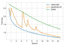
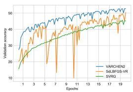
Figure 1: Evolution of the training loss (left) and the validation accuracy (right) for training a modified DavidNet on CIFAR-10.

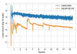
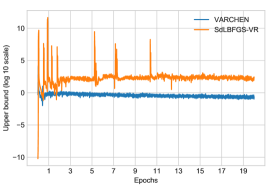
Figure 2: Evolution of the lower bound on the smallest eigenvalue $\lambda_{k}$ (left) and the upper bound on the largest eigenvalue $\Lambda_{k}$ (right) on a base 10 logarithmic scale for training a modified DavidNet on CIFAR-10.

Figure 1 shows that VARCHEN outperforms SdLBFGS-VR for the training loss minimization task, and both outperform SVRG. VARCHEN has an edge over SdLBFGS-VR in terms of the validation accuracy, and both outperform SVRG. More importantly, the performance of VARCHEN is more consistent than that of SdLBFGS-VR, displaying a smoother, less oscillatory behaviour. To further investigate this observation, we plot the evolution of $\Lambda_{k}$ and $\lambda_{k}$ as shown in Figure 2. We see that the estimate of the lower bound on the smallest eigenvalue is smaller for SdLBFGS-VR compared to VARCHEN. We also notice that the estimate of the upper bound of the largest eigenvalue of $H_{k}$ takes even more extreme values for SdLBFGS-VR compared to VARCHEN. The extreme values $\lambda_{k}$ and $\Lambda_{k}$ reflect an ill-conditioning problem encountered when using SdLBFGS-VR and we believe that it explains the extreme oscillations in the performance of SdLBFGS-VR.

6 Conclusion

We used the stochastic damped L-BFGS algorithm in a nonconvex setting, where there are no guarantees that $H_{k}$ remains well-conditioned and numerically nonsingular throughout. We introduced a new stochastic damped L-BFGS algorithm that monitors the quality of $H_{k}$ during the optimization by maintaining bounds on its largest and smallest eigenvalues. Our work is the first to address the Hessian singularity problem by approximating and leveraging such bounds. Moreover, we proposed a new initial inverse Hessian approximation that results in a smoother, less oscillatory training loss and validation accuracy evolution. Additionally, we used variance reduction in order to improve the quality of the curvature approximation and accelerate convergence. Our algorithm converges almost-surely to a stationary point and numerical experiments have shown that it is more robust to ill-conditioned problems and more suitable to the highly nonconvex context of deep learning than SdLBFGS-VR. We consider this work to be a first step towards the use of bounds estimates to control the quality of the Hessian approximation in approximate second-order algorithms. Future work should aim to improve the quality of these bounds and explore another form of variance reduction that consists of adaptive sampling (Jalilzadeh et al., 2018; Bollapragada et al., 2018; Bollapragada and Wild, 2019).

Appendix A Proofs

Proof A.1.

​ of Lemma 3.1. First notice that

$$\gamma\|s\|^{2}\leq s^{\top}y\leq\|s\|\|y\|,\quad\text{and thus}\quad\|s\|\leq\frac{1}{\gamma}\|y\|.$$

Therefore,

$$\frac{1}{\|s\|\|y\|}\leq\rho\leq\frac{1}{\gamma}\frac{1}{\|s\|^{2}}.$$ (12)

Since $A$ is a real symmetric matrix, the spectral theorem states that its eigenvalues are real and it can be diagonalized by an orthogonal matrix. That means that we can find $n$ orthogonal eigenvectors and $n$ eigenvalues counted with multiplicity.

Consider first the special case where $s$ and $y$ are collinear, i.e. there exists $\theta>0$ such that $y=\theta s$. Any vector such that $u\in s^{\perp}$, where $s^{\perp}=\{x\in\mathbb{R}^{n}:x^{\top}s=0\}$, is an eigenvector of $A$ associated with the eigenvalue $\mu$ of multiplicity $n-1$. Moreover, $s^{\top}y=\theta\|s\|^{2}=\|s\|\|y\|$, $\rho=1/(\theta\|s\|^{2})$ and we have

$$As=\left[\mu\left(I-\rho\theta ss^{\top}\right)^{2}+\rho ss^{\top}\right]s=\left[\mu\left(1-\rho\theta\|s\|^{2}\right)^{2}+\rho\|s\|^{2}\right]s=\rho\|s\|^{2}s.$$

Let us call $\lambda=\rho\|s\|^{2}$, the eigenvalue associated with eigenvector $s$. From (12) and $\|y\|\leq L_{y}\|s\|$, we deduce that

$$\frac{1}{L_{y}}\leq\lambda\leq\frac{1}{\gamma}.$$

Suppose now that $s$ and $y$ are linearly independent. Any $u$ such that $u^{\top}s=0=u^{\top}y$ satisfies $Au=\mu u$. This provides us with a ($n-2$)-dimensional eigenspace $S$, associated to the eigenvalue $\mu$ of multiplicity $n-2$. Note that

$$As =\rho\|s\|^{2}\ (1+\mu\rho\|y\|^{2})s-\rho\|s\|^{2}\mu y,$$

$$Ay =s.$$

Thus neither $s$ nor $y$ is an eigenvector of $A$. Now consider an eigenvalue $\lambda$ associated with an eigenvector $u$, such that $u\in S^{\perp}$. Since $s$ and $y$ are linearly-independent, we can search for $u$ of the form $u=s+\beta y$ with $\beta>0$. The condition $Au=\lambda u$ yields

$$\rho\|s\|^{2}\ (1+\mu\rho\|y\|^{2})+\beta =\lambda,$$

$$-\rho\|s\|^{2}\mu =\lambda\beta.$$

We eliminate $\beta=\lambda-\rho\|s\|^{2}\ (1+\mu\rho\|y\|^{2})$ and obtain

$$p(\lambda)=0,$$

where

$$p(\lambda)=\lambda^{2}-\lambda\rho\|s\|^{2}\ (1+\mu\rho\|y\|^{2})+\rho\|s\|^{2}\mu.$$

The roots of $p$ must be the two remaining eigenvalues $\lambda_{1}\leq\lambda_{2}$ that we are looking for. In order to establish the lower bound, we need a lower bound on $\lambda_{1}$ whereas to establish the upper bound, we need an upper bound on $\lambda_{2}$.

On the one hand, let $l$ be the tangent to the graph of $p$ at $\lambda=0$, defined by

$$l(\lambda)=p(0)+p^{\prime}(0)\lambda=\mu\rho\|s\|^{2}-\lambda\rho\|s\|^{2}\left(1+\mu\rho\|y\|^{2}\right).$$

Its unique root is

$$\bar{\lambda}=\frac{\mu}{1+\mu\rho\|y\|^{2}}.$$

From (12) and since $\|y\|\leq L_{y}\|s\|$, we deduce that

$$\bar{\lambda}\geq\frac{\mu}{1+\frac{\mu}{\gamma}\frac{\|y\|^{2}}{\|s\|^{2}}}\geq\frac{\mu}{1+\frac{\mu}{\gamma}L_{y}^{2}}.$$

Since $p$ is convex, it remains above its tangent, and $\bar{\lambda}\leq\lambda_{1}$.

Finally,

$$\lambda_{\min}(A)\geq\min\left(\frac{1}{L_{y}},\frac{\mu}{1+\frac{\mu}{\gamma}L_{y}^{2}}\right)>0.$$

This establishes the lower bound.

On the other hand, the discriminant $\Delta=\rho^{2}\|s\|^{4}(1+\mu\rho\|y\|^{2})^{2}-4\rho\|s\|^{2}\mu$ must be nonnegative since $A$ is real symmetric, and its eigenvalues are real. We have

$$\lambda_{2}=\frac{\rho\|s\|^{2}(1+\mu\rho\|y\|^{2})+\sqrt{\rho^{2}\|s\|^{4}(1+\mu\rho\|y\|^{2})^{2}-4\rho\|s\|^{2}\mu}}{2}.$$

For any positive $a$ and $b$ such that $a^{2}-b>0$, we have $\sqrt{a^{2}-b}\leq a-\tfrac{b}{2a}$. Thus,

$$\lambda_{2}\leq\rho\|s\|^{2}(1+\mu\rho\|y\|^{2})-\frac{\mu}{1+\mu\rho\|y\|^{2}}.$$

From (12), we deduce that

$$\lambda_{2}\leq\frac{1}{\gamma}+\frac{\mu}{\gamma^{2}}\frac{\|y\|^{2}}{\|s\|^{2}}-\frac{\mu}{1+\frac{\mu}{\gamma}\frac{\|y\|^{2}}{\|s\|^{2}}}.$$

And since $\|y\|\leq L_{y}\|s\|$, it follows

$$\lambda_{2}\leq\frac{1}{\gamma}+\frac{\mu}{\gamma^{2}}L_{y}^{2}-\frac{\mu}{1+\frac{\mu}{\gamma}L_{y}^{2}}.$$

Finally,

$$\lambda_{\max}(A)\leq\max\left(\frac{1}{\gamma},\frac{1}{\gamma}+\frac{\mu}{\gamma^{2}}L_{y}^{2}-\frac{\mu}{1+\frac{\mu}{\gamma}L_{y}^{2}}\right),$$

which establishes the upper bound.

Proof A.2.

​ of Theorem 3.2. Consider one damped BFGS update using $s$ and $y$ defined in (5) and $\hat{y}_{k}$ defined in (7), i.e, $p=1$,

$$H_{k+1}=\hat{V}_{k}H_{k+1}^{0}\hat{V}_{k}^{\top}+\hat{\rho}_{k}s_{k}s_{k}^{\top},\quad\text{where}\quad\hat{\rho}_{k}=1/s_{k}^{\top}\hat{y}_{k},\quad\hat{V}_{k}=I-\hat{\rho}_{k}s_{k}\hat{y}_{k}^{\top}.$$

Let $0<\mu_{1}:=\lambda_{\min}(H_{k+1}^{0})\leq\mu_{2}:=\lambda_{\max}(H_{k+1}^{0})$. We have

$$\lambda_{\min}(\mu_{1}\hat{V}_{k}\hat{V}_{k}^{\top}+\hat{\rho}_{k}s_{k}s_{k}^{\top})\leq\lambda_{\min}(H_{k+1})\leq\lambda_{\max}(H_{k+1})\leq\lambda_{\max}(\mu_{2}\hat{V}_{k}\hat{V}_{k}^{\top}+\hat{\rho}_{k}s_{k}s_{k}^{\top}).$$ (13)

Let us show that we can apply Lemma 3.1 to

$$A_{1}:=\mu_{1}\hat{V}_{k}\hat{V}_{k}^{\top}+\hat{\rho}_{k}s_{k}s_{k}^{\top}\quad\text{and}\quad A_{2}:=\mu_{2}\hat{V}_{k}\hat{V}_{k}^{\top}+\hat{\rho}_{k}s_{k}s_{k}^{\top}.$$

From (9), we obtain

$$s_{k}^{\top}\hat{y}_{k}\geq\eta\lambda_{\min}(B_{k+1}^{0})\|s_{k}\|^{2}=\frac{\eta}{\lambda_{\max}(H_{k+1}^{0})}\|s_{k}\|^{2}=\frac{\eta}{\mu_{2}}\|s_{k}\|^{2}.$$

Assumption 2 yields

$$\|\hat{y}_{k}\|=\|\theta_{k}y_{k}+(1-\theta_{k})B_{k+1}^{0}s_{k}\|\leq\|y_{k}\|+\|B_{k+1}^{0}s_{k}\|\leq(L_{g}+1/\mu_{1})\|s_{k}\|.$$

Therefore, we can first apply Lemma 3.1 with $s_{k}$, $\hat{y}_{k}$, $\gamma=\eta/\mu_{2}>0$, $L_{y}=L_{g}+1/\mu_{1}>0$ and $\mu=\mu_{1}>0$ for $A_{1}$, and apply it again with $\mu=\mu_{2}>0$ for $A_{2}$. Let $L_{1}:=L_{g}+1/\mu_{1}$. Lemma 3.1 and (13) yield

$$\lambda_{\min}(H_{k+1}) \geq\min\left(\frac{1}{L_{1}},\frac{\mu_{1}}{1+\frac{\mu_{1}\mu_{2}}{\eta}L_{1}^{2}}\right)>0,$$

$$\lambda_{\max}(H_{k+1}) \leq\frac{\mu_{2}}{\eta}+\max\left(0,\frac{\mu_{2}^{3}}{\eta^{2}}L_{1}^{2}-\frac{\mu_{2}}{1+\frac{\mu_{2}^{2}}{\eta}L_{1}^{2}}\right).$$

Now, consider the case where $p>1$ and let

$$H_{k+1}^{(h+1)}:=\hat{V}_{k-h}H_{k+1}^{(h)}\hat{V}_{k-h}^{\top}+\hat{\rho}_{k-h}s_{k-h}s_{k-h}^{\top},\quad 0\leq h\leq p-1,$$

where

$$H^{(p)}_{k+1}:=H_{k+1},\quad\hat{\rho}_{k-h}=1/s_{k-h}^{\top}\hat{y}_{k-h},\quad\hat{V}_{k}=I-\hat{\rho}_{k-h}s_{k-h}\hat{y}_{k-h}^{\top}.$$

Similarly to the case $p=1$, we may write

$$\lambda_{\min}(H_{k+1}^{(h+1)}) \geq\lambda_{\min}(\mu_{1}^{(h)}\hat{V}_{k-h}\hat{V}_{k-h}^{\top}+\hat{\rho}_{k-h}s_{k-h}s_{k-h}^{\top}),\qquad\mu_{1}^{(h)} :=\lambda_{\min}(H_{k+1}^{(h)}),$$

$$\lambda_{\max}(H_{k+1}^{(h+1)}) \leq\lambda_{\max}(\mu_{2}^{(h)}\hat{V}_{k-h}\hat{V}_{k-h}^{\top}+\hat{\rho}_{k-h}s_{k-h}s_{k-h}^{\top}),\qquad\mu_{2}^{(h)} :=\lambda_{\max}(H_{k+1}^{(h)}).$$

Assume by recurrence that $0<\mu_{1}^{(h)}\leq\mu_{2}^{(h)}$. We show that we can apply Lemma 3.1 to

$$A_{1}^{(h)}:=\mu_{1}^{(h)}\hat{V}_{k-h}\hat{V}_{k-h}^{\top}+\hat{\rho}_{k-h}s_{k-h}s_{k-h}^{\top}\quad\text{and}\quad A_{2}^{(h)}:=\mu_{2}^{(h)}\hat{V}_{k-h}\hat{V}_{k-h}^{\top}+\hat{\rho}_{k-h}s_{k-h}s_{k-h}^{\top}.$$

From (9), we have

$$s_{k-h}^{\top}\hat{y}_{k-h}\geq\eta\lambda_{\min}(B_{k-h+1}^{0})\|s_{k-h}\|^{2}=\frac{\eta}{\lambda_{\max}(H_{k-h+1}^{0})}\|s_{k-h}\|^{2}.$$

Using Assumption 2,

$$\|\hat{y}_{k-h}\|=\|\theta_{k-h}y_{k-h}+(1-\theta_{k-h})B_{k-h+1}^{0}s_{k-h}\|\leq L_{g}\|s_{k-h}\|+\|B_{k-h+1}^{0}s_{k-h}\|,$$

so that

$$\|\hat{y}_{k-h}\|\leq(L_{g}+\frac{1}{\lambda_{\min}(H_{k-h+1}^{0})})\|s_{k-h}\|.$$

We first apply Lemma 3.1 with $s=s_{k-h}$, $y=\hat{y}_{k-h}$, $\gamma=\eta/\lambda_{\max}(H_{k-h+1}^{0})>0$, $L_{y}=L_{g}+1/\lambda_{\min}(H_{k-h+1}^{0})>0$ and $\mu=\mu_{1}^{(h)}>0$ for $A_{1}^{(h)}$, and apply it a second time with $\mu=\mu_{2}^{(h)}>0$ for $A_{2}^{(h)}$. Let $L_{k-h+1}:=L_{g}+1/\lambda_{\min}(H_{k-h+1}^{0})$ and $\gamma_{k-h+1}=\eta/\lambda_{\max}(H_{k-h+1}^{0})$. Then we have

$$\lambda_{\min}(H_{k+1}^{(h+1)})\geq\min\left(\frac{1}{L_{k-h+1}},\frac{\lambda_{\min}(H_{k+1}^{(h)})}{1+\frac{\lambda_{\min}(H_{k+1}^{(h)})}{\gamma_{k-h+1}}(L_{k-h+1})^{2}}\right),$$ (14)

and

$$\lambda_{\max}(H_{k+1}^{(h+1)})\leq\frac{1}{\gamma_{k-h+1}}+\max\left(0,\frac{\lambda_{\max}(H_{k+1}^{(h)})}{\gamma_{k-h+1}^{2}}L_{k-h+1}^{2}-\frac{\lambda_{\max}(H_{k+1}^{(h)})}{1+\frac{\lambda_{\max}(H_{k+1}^{(h)})}{\gamma_{k-h+1}}L_{k-h+1}^{2}}\right).$$ (15)

It is clear that we can obtain the lower bound on $\lambda_{\min}(H_{k+1})$ recursively using (14). Obtaining the upper bound on $\lambda_{\max}(H_{k+1})$ using (15) is trickier. However, we notice that inequality (15) implies

$$\lambda_{\max}(H_{k+1}^{(h+1)})\leq\frac{1}{\gamma_{k-h+1}}+\max\left(0,\frac{\lambda_{\max}(H_{k+1}^{(h)})}{\gamma_{k-h+1}^{2}}L_{k-h+1}^{2}-\frac{\lambda_{\min}(H_{k+1}^{(h)})}{1+\frac{\lambda_{\max}(H_{k+1}^{(h)})}{\gamma_{k-h+1}}L_{k-h+1}^{2}}\right).$$

This upper bound is less tight but it allows us to bound $\lambda_{\max}(H_{k+1})$ recursively.

Appendix B Algorithms

The Two-loop recursion algorithm for evaluating the Hessian-gradient product is given by Algorithm 2.

Algorithm 2 Two-loop recursion algorithm for Hessian-gradient product computation

0:  Current iterate $x_{k}$, $g(x_{k},\xi_{k})$, $\hat{\rho}_{i}=1/s_{i}^{\top}\hat{y}_{i}$, $s_{i}$, $\hat{y}_{i}$ for $i\in\{k-p,\ldots,k-1\}$.

1:  Define $g=g(x_{k},\xi_{k})$

2:  for $i=k-1,k-2,\ldots,k-p$ do

3:     Compute $\nu_{i}=\hat{\rho}_{i}s_{i}^{\top}g$

4:     Compute $g=g-\nu_{i}\hat{y}_{i}$

5:  Compute $q=H_{k}^{0}\,g$ using (10).

6:  for $i=k-p,k-p+1,\ldots,k-1$ do

7:     Compute $\mu=\hat{\rho}_{i}\hat{y}_{i}^{\top}q$

8:     Compute $q=q+(\nu_{i}-\mu)s_{i}$

9:  Return $q=H_{k}\,g(x_{k},\xi_{k})$

Appendix C Experimental Setting

CIFAR-10 is a dataset that contains $60,000$ colour images with labels in $10$ classes (airplane, automobile, bird, cat, deer, dog, frog, horse, ship, and truck), each containing $6,000$ images. We use $50,000$ images for the training task and $10,000$ images for the validation task.

Details of the experiments:

• We apply our Hessian norm control using the bound on the maximum and the minimum eigenvalues of $H_{k+1}$, where the latter is equivalent to controlling $\|B_{k+1}\|$;

• In the definition of $H_{k+1}^{0}$ in (10), we choose $\underline{\gamma}_{k+1}$ and $\overline{\gamma}_{k+1}$ constant;

• The numerical values for all algorithms are the ones that yielded the best results among all sets of values that we experimented with.

Numerical values:

• For all algorithms: we train the network for $20$ epochs and use a batch size of $256$ samples;

• For SVRG, we choose a step size equal to $0.001$;

• For both SdLBFGS-VR and Algorithm 1, the memory parameter $p=10$, the minimal scaling parameter $\underline{\gamma}_{k+1}=0.1$ for all $k$, the constant step size $\alpha_{k}=0.1$ and $\eta=0.25$;

• For Algorithm 1, we use a maximal scaling parameter $\overline{\gamma}_{k+1}=10^{5}$ for all $k$, a lower bound limit $\lambda_{\min}=10^{-5}$ and an upper bound limit $\lambda_{\max}=10^{5}$.

References

• Amari (1998) Shun-Ichi Amari. Natural gradient works efficiently in learning. Neural computation, 10(2):251–276, 1998.
• Bollapragada and Wild (2019) Raghu Bollapragada and Stefan M Wild. Adaptive sampling quasi-Newton methods for derivative-free stochastic optimization. arXiv preprint arXiv:1910.13516, 2019.
• Bollapragada et al. (2018) Raghu Bollapragada, Dheevatsa Mudigere, Jorge Nocedal, Hao-Jun Michael Shi, and Ping Tak Peter Tang. A progressive batching l-bfgs method for machine learning. arXiv preprint arXiv:1802.05374, 2018.
• Bordes et al. (2009) Antoine Bordes, Léon Bottou, and Patrick Gallinari. SGD-QN: Careful quasi-Newton stochastic gradient descent. Journal of Machine Learning Research, 10(Jul):1737–1754, 2009.
• Bottou (2010) Léon Bottou. Large-scale machine learning with stochastic gradient descent. In Proceedings of COMPSTAT’2010, pages 177–186. Springer, 2010.
• Bottou et al. (2018) Léon Bottou, Frank E Curtis, and Jorge Nocedal. Optimization methods for large-scale machine learning. Siam Review, 60(2):223–311, 2018.
• Byrd et al. (2016) Richard H Byrd, Samantha L Hansen, Jorge Nocedal, and Yoram Singer. A stochastic quasi-Newton method for large-scale optimization. SIAM Journal on Optimization, 26(2):1008–1031, 2016.
• Chen et al. (2019) Huiming Chen, Ho-Chun Wu, Shing-Chow Chan, and Wong-Hing Lam. A stochastic quasi-Newton method for large-scale nonconvex optimization with applications. IEEE Transactions on Neural Networks and Learning Systems, 2019.
• Dembo et al. (1982) Ron S Dembo, Stanley C Eisenstat, and Trond Steihaug. Inexact Newton methods. SIAM Journal on Numerical analysis, 19(2):400–408, 1982.
• Dennis and Moré (1974) John E Dennis and Jorge J Moré. A characterization of superlinear convergence and its application to quasi-Newton methods. Mathematics of computation, 28(126):549–560, 1974.
• Dennis Jr and Schnabel (1996) John E Dennis Jr and Robert B Schnabel. Numerical methods for unconstrained optimization and nonlinear equations, volume 16. SIAM, Philadelphia, PA, 1996.
• Duchi et al. (2011) John Duchi, Elad Hazan, and Yoram Singer. Adaptive subgradient methods for online learning and stochastic optimization. Journal of machine learning research, 12(7), 2011.
• Fang et al. (2018) Cong Fang, Chris Junchi Li, Zhouchen Lin, and Tong Zhang. Spider: Near-optimal non-convex optimization via stochastic path-integrated differential estimator. In Advances in Neural Information Processing Systems, pages 689–699, 2018.
• Fletcher (1970) Roger Fletcher. A new approach to variable metric algorithms. The computer journal, 13(3):317–322, 1970.
• Gower et al. (2016) Robert Gower, Donald Goldfarb, and Peter Richtárik. Stochastic block BFGS: Squeezing more curvature out of data. In International Conference on Machine Learning, pages 1869–1878, 2016.
• Jalilzadeh et al. (2018) Afrooz Jalilzadeh, Angelia Nedić, Uday V Shanbhag, and Farzad Yousefian. A variable sample-size stochastic quasi-Newton method for smooth and nonsmooth stochastic convex optimization. In 2018 IEEE Conference on Decision and Control (CDC), pages 4097–4102. IEEE, 2018.
• Johnson and Zhang (2013) Rie Johnson and Tong Zhang. Accelerating stochastic gradient descent using predictive variance reduction. In Advances in neural information processing systems, pages 315–323, 2013.
• Kingma and Ba (2015) Diederik P Kingma and Jimmy Ba. Adam: A method for stochastic optimization. In International Conference on Learning Representations, 2015.
• Krizhevsky (2009) Alex Krizhevsky. Learning multiple layers of features from tiny images. Technical report, University of Toronto, 2009.
• LeCun et al. (2010) Yann LeCun, Corinna Cortes, and CJ Burges. MNIST handwritten digit database. ATT Labs [Online]. Available: http://yann.lecun.com/exdb/mnist, 2, 2010.
• Lewis et al. (2004) David D Lewis, Yiming Yang, Tony G Rose, and Fan Li. Rcv1: A new benchmark collection for text categorization research. Journal of machine learning research, 5(Apr):361–397, 2004.
• Liu and Nocedal (1989) Dong C Liu and Jorge Nocedal. On the limited memory BFGS method for large scale optimization. Mathematical programming, 45(1-3):503–528, 1989.
• Mokhtari and Ribeiro (2014) Aryan Mokhtari and Alejandro Ribeiro. Res: Regularized stochastic BFGS algorithm. IEEE Transactions on Signal Processing, 62(23):6089–6104, 2014.
• Moritz et al. (2016) Philipp Moritz, Robert Nishihara, and Michael Jordan. A linearly-convergent stochastic L-BFGS algorithm. In Artificial Intelligence and Statistics, pages 249–258, 2016.
• Nesterov (1983) Yurii E Nesterov. A method for solving the convex programming problem with convergence rate O(1/k2)𝑂1superscript𝑘2{O}(1/k^{2}). In Dokl. akad. nauk Sssr, volume 269, pages 543–547, 1983.
• Nguyen et al. (2017) Lam M Nguyen, Jie Liu, Katya Scheinberg, and Martin Takáč. Sarah: A novel method for machine learning problems using stochastic recursive gradient. arXiv preprint arXiv:1703.00102, 2017.
• Nocedal (1980) Jorge Nocedal. Updating quasi-Newton matrices with limited storage. Mathematics of computation, 35(151):773–782, 1980.
• Polyak (1964) Boris T Polyak. Some methods of speeding up the convergence of iteration methods. USSR Computational Mathematics and Mathematical Physics, 4(5):1–17, 1964.
• Powell (1978) Michael JD Powell. Algorithms for nonlinear constraints that use Lagrangian functions. Mathematical programming, 14(1):224–248, 1978.
• Robbins and Monro (1951) Herbert Robbins and Sutton Monro. A stochastic approximation method. The annals of mathematical statistics, pages 400–407, 1951.
• Schraudolph et al. (2007) Nicol N Schraudolph, Jin Yu, and Simon Günter. A stochastic quasi-Newton method for online convex optimization. In Artificial intelligence and statistics, pages 436–443, 2007.
• Tieleman and Hinton (2012) Tijmen Tieleman and Geoffrey Hinton. Rmsprop: Divide the gradient by a running average of its recent magnitude. coursera: Neural networks for machine learning. COURSERA Neural Networks Mach. Learn, 2012.
• Wang et al. (2017) Xiao Wang, Shiqian Ma, Donald Goldfarb, and Wei Liu. Stochastic quasi-Newton methods for nonconvex stochastic optimization. SIAM Journal on Optimization, 27(2):927–956, 2017.
• Wang et al. (2019) Zhe Wang, Kaiyi Ji, Yi Zhou, Yingbin Liang, and Vahid Tarokh. Spiderboost and momentum: Faster variance reduction algorithms. In Advances in Neural Information Processing Systems, pages 2406–2416, 2019.
• Wolfe (1969) Philip Wolfe. Convergence conditions for ascent methods. SIAM Review, 11(2):226–235, 1969.
• Wolfe (1971) Philip Wolfe. Convergence conditions for ascent methods II: Some corrections. SIAM Review, 13(2):185–188, 1971.
• Yousefian et al. (2017) Farzad Yousefian, Angelia Nedić, and Uday V Shanbhag. A smoothing stochastic quasi-Newton method for non-Lipschitzian stochastic optimization problems. In 2017 Winter Simulation Conference (WSC), pages 2291–2302. IEEE, 2017.