Angular momentum anisotropy of Dirac carriers: A new twist in graphene

Abstract

Dirac carriers in graphene are commonly characterized by a pseudospin degree of freedom, arising from the degeneracy of the two inequivalent sublattices. The inherent chirality of the quasiparticles leads to a topologically non-trivial band structure, where the in-plane components of sublattice spin and momentum are intertwined. Equivalently, sublattice imbalance is intimately connected with angular momentum, inducing a torque of opposite sign at each Dirac point. In this work we develop an intuitive picture that associates sublattice spin and winding number with angular momentum. We develop a microscopic perturbative model to obtain the finite angular momentum contributions along the main crystallographic directions. Our results can be employed to determine the angular dependence of the $g$ factor and of light absorption in honeycomb bipartite structures.

I Introduction

The linear dispersion at the Fermi level of graphene is cognate with the Dirac cones of massless relativistic particles Novoselov et al. (2005), motivating extensive research towards the parallelism with relativistic quantum mechanics and quantum electrodynamics (QED) in solid-state materials Katsnelson et al. (2006); Geim and Novoselov (2010); Nair et al. (2008); Katsnelson and Novoselov (2007); Giuliani et al. (2012); Marino et al. (2015); Golub et al. (2020). In this Dirac-type model, the notion of sublattice (SL) spin takes the role of real spin, with “up” and “down” states being associated with the two SL components that constitute the honeycomb structure. The inherent chirality of the Dirac carriers leads to a topologically non-trivial band structure, where the related edge’s helicity gives rise to the spin Hall insulator Kane and Mele (2005a, b); Sichau et al. (2019). The presence of a pseudospin degree of freedom in the Hamiltonian allows a parallelism between its torque and that of the angular momentum Mecklenburg and Regan (2011); Soodchomshom (2013), where an experimental connection has been realized only in photonic graphene Song et al. (2015); Liu et al. (2018, 2020).

In this work we evaluate the constants of motion and provide an intuitive connection between SL spin and angular momentum in the neighborhood of the Fermi energy. We develop a microscopic perturbative model to obtain the corrections to the angular momentum $\vec{L}$ in terms of atomic parameters. We consider band hybridization, spin-orbit coupling (SOC) and Bychkov-Rashba effect, and obtain a peculiar anisotropy in the corrections, owing to the relation of $\hat{L}$ and SL spin. These corrections have been verified in large graphene samples, by measuring the g-factor corrections Prada et al. (2020).

This paper is organized as follows: First we employ symmetry arguments to analyze the low-lying quasiparticle Hamiltonian. We examine perturbatively the $d$-orbital contribution to the $\pi$-bands ($l=2$, $m_{l}=\pm 1$), and calculate the correction to the angular momentum. Finally, we include perturbatively the mixing with the $\sigma$-band ($l=1$, $m_{l}=\pm 1$) via atomic SOC and Bychkov-Rashba interaction, and obtain the angular momentum corrections in terms of atomic parameters.

II Band mixing and hybridization

II.1 Dirac electrons to lowest order: $\langle\hat{L}\rangle=0$ orbitals

Dirac electrons near the Fermi edge are commonly described by $\pi$ orbitals within a nearest neighbors (NN) tight-binding model Castro Neto et al. (2009); Katsnelson (2012). The two sublattices that constitute the honeycomb structure lead to two energy bands, whose interplay yields a conical quasiparticle spectrum. The concept of isospin or SL spin is commonly introduced, where the $z$ component, $\sigma_{z}$, accounts for the SL occupation imbalance. At the Dirac points (DPs), the quasiparticle Dirac-type Hamiltonian reads as Kane and Mele (2005a); Mecklenburg and Regan (2011); Castro Neto et al. (2009); Katsnelson (2012):

$$\hat{H}_{0}=\hbar v_{F}\left(\tau q_{x}\hat{\sigma}_{x}+q_{y}\hat{\sigma}_{y}\right)+\hat{\lambda}\hat{\sigma}_{z}=\hbar v_{F}\hat{\vec{\sigma}}_{\tau}^{\parallel}\hat{\vec{q}}+\hat{\lambda}\hat{\sigma}_{z},$$ (1)

where we have assigned the valley index $\tau$ = 1 and $\tau$ = -1, respectively, to the DPs, $K$ and $K^{\prime}$, and $\vec{q}=(q_{x},q_{y})$ is the small vector off the nearest DP. Here, $v_{F}\simeq 10^{6}$ ms^-1 the Fermi velocity, $\hat{s}_{\alpha}$, $\hat{\sigma}_{\alpha}$ are the Pauli matrices representing the electron spin and sublattice-spin, respectively, and we have defined the vector $\hat{\vec{\sigma}}_{\tau}^{\parallel}\equiv(\tau\hat{\sigma}_{x},\hat{\sigma}_{y})$. The first term originates from the quantum mechanical hopping between the two sublattices and tends to align $\vec{q}$ and $\hat{\vec{\sigma}}_{\tau}^{\parallel}$. In spite of involving the Pauli matrices, it is a scalar (see Appendix A). The second term can be, however, a scalar, in the case of a Kane-Mele SOC Kane and Mele (2005a) ($\hat{\lambda}\hat{\sigma}_{z}=\tau\lambda_{I}\hat{s}_{z}\hat{\sigma}_{z}$) or a pseudoscalar, in case of a staggered sublattice potential Semenoff (1984), $\hat{\lambda}\hat{\sigma}_{z}=\varepsilon_{AB}\hat{\sigma}_{z}=(\varepsilon_{A}-\varepsilon_{B})\hat{\sigma}_{z}/2$, owing to the broken parity symmetry. The distinction is important, as it is only in the former case where a direct analogy with the equations of a dipole in a magnetic field can be made. To lowest order, the eigenenergies of (1) are given by:

$$\varepsilon_{\pm}=\pm\sqrt{(\hbar v_{F}|q|)^{2}+\lambda^{2}}.$$ (2)

The corresponding eigenstates are commonly given in terms of the dominant ($p_{z}$-orbital) contribution at sublattices $A$ and $B$ for $q\neq 0$,

$$|\varphi^{(0)}_{\pm}\rangle\simeq c_{A}|p_{z}^{A}\rangle+c_{B}|p_{z}^{B}\rangle,\ \frac{c_{B}}{c_{A}}=\pm e^{i\tau\varphi_{q}},\ \varphi_{q}=\arctan{\frac{q_{y}}{q_{x}}}.$$ (3)

The relative phase between the two sublattice components $\tau\varphi_{q}$ results indeed in a Berry phase Shapere and Wilczek (1989), and determines the direction of the associated SL spin Ando et al. (1998); McEuen et al. (1999), in analogy with chirality and charge conjugation in QED Katsnelson and Novoselov (2007); Katsnelson et al. (2006). At the critical point $q=0$, however, the SL spin components are decoupled, and the solutions depend on the (pseudo) scalar nature of the mass term. A scalar, Kane-Mele SOC results in decoupled bispinors where the conduction band in $K$ relates to the valence band in $K^{\prime}$, leading to the spin-Hall effect Kane and Mele (2005b, a). On the other hand, the staggered potential results in a trivial insulator, with the peculiarity of pseudoscalar eigenvalues at the DPs.

We evaluate now the expectation value of the SL spin components. For the states of (3), we obtain:

$$\sigma^{0}_{z} \equiv \langle\varphi^{(0)}_{\pm}|\hat{\sigma}_{z}|\varphi^{(0)}_{\pm}\rangle=|c_{A}|^{2}-|c_{B}|^{2},$$

$$\langle\hat{\vec{\sigma}}_{\tau}^{\parallel}\rangle^{0} \equiv \left(\begin{array}[]{c}\langle\tau\hat{\sigma}_{x}\rangle\\ \langle\hat{\sigma}_{y}\rangle\end{array}\right)\simeq\pm\left(\begin{array}[]{c}\tau\cos{\varphi_{q}\tau}\\ \sin{\varphi_{q}\tau}\end{array}\right)=\pm\frac{\tau}{q}\left(\begin{array}[]{c}q_{x}\\ q_{y}\end{array}\right),$$ (10)

where we have used $2|c_{A}|^{2}\simeq 1$. A three-component axial vector $\vec{\sigma}_{\tau}$ was already identified with the real angular momentum Mecklenburg and Regan (2011); Soodchomshom (2013). Doing so, however, results in unphysical interpretations for the equations of motion or the conserved quantities, owing to the different physical meaning of the different components. Here we aim at bringing clarity and physical meaning to the connection between the angular momentum components $\hat{L}_{\parallel},\hat{L}_{z}$, and $\vec{\sigma}_{\tau}^{\parallel}$, $\sigma_{z}$. For the easy axis, the $z$ component of angular momentum is associated with the pseudoscalar $\tau\sigma_{z}$:

$$\left[\hat{H}_{0},\hat{L}_{z}\right]=-\frac{\hbar}{2}\left[\hat{H}_{0},\hat{\sigma}_{z\tau}\right]=-i\hbar v_{F}\hat{\vec{\sigma}}_{\tau}^{\parallel}\times\hat{\vec{p}}=-i\hbar\dot{\vec{r}}\times\hat{\vec{p}},$$

where we have used that $\dot{\vec{r}}=(i/\hbar)[\hat{H}_{0},\hat{\vec{r}}]=v_{F}\hat{\vec{\sigma}}_{\tau}^{\parallel}$, that is, $\hat{\vec{\sigma}}_{\tau}^{\parallel}$ is aligned with the velocity Soodchomshom (2013). As Mecklenburg et al. already pointed out Mecklenburg and Regan (2011), this implies that the constant of motion is $2{L}_{z}+\hbar\tau{\sigma}_{z}$, which we generalize to bilayer graphene’s Dirac Hamiltonians in terms of the winding number $\nu$ (see Appendix B) as:

$$\frac{\rm d}{\rm dt}\left(2{L}_{z}+\nu\hbar\tau{\sigma}_{z}\right)=0.$$ (12)

That means that sublattice imbalance induces a torque in the quasiparticle spectrum of opposite sign on each valley. Likewise, a finite $L_{z}$ induces a sublattice imbalance of opposite sign on each valley. The same line of argument can be used in the presence of a Kane-Mele term, where $\langle\tau\sigma_{z}\rangle$ has different sign for electrons with opposite spin, resulting in splitting of left- or right-propagating states Hasan and Kane (2010); Kane and Mele (2005a). This peculiarity is reflected in the band mixing, as will be detailed in the next section: Dirac electrons on a given SL (say $A$) and valley couple only to clockwise rotating orbitals, and the converse is true for those on SL $B$.

An intuitive picture can be given in terms of the winding number: in monolayer (bilayer) graphene, the Berry phase is $\pi$ (2$\pi$), yielding a $\nu=$1 (2) winding number. This means that an adiabatic closed contour in momentum space the SL spin “winds ”around the origin once (twice), just like momentum does Asbóth et al. (2006); Prada et al. (2011) [see Fig. 1(c)]. This rotational in momentum space can be then intuitively associated with a torque and, hence, its path integral should be related to the angular momentum.

For the in-plane components we may define an in-plane pseudovector operator

$$\hat{\vec{\mathcal{L}}}_{\parallel}=(\hat{\lambda}/\hbar v_{F})\hat{\vec{r}}\times\hat{\vec{u}}_{z},$$ (13)

that could relate to in-plane angular momentum. With this definition, we obtain:

$$\frac{\rm d}{{\rm d}t}\hat{\vec{\mathcal{L}}}_{\parallel}=\frac{i}{\hbar}\left[\hat{H}_{0},\hat{\vec{\mathcal{L}}}_{\parallel}\right]=-\hat{\lambda}\left(\begin{array}[]{c}-\hat{\sigma}_{y}\\ \tau\hat{\sigma}_{x}\end{array}\right)=\hat{\lambda}\hat{\vec{\sigma}}_{\tau}^{\parallel}\times\hat{\vec{u}}_{z}.$$ (14)

On the other hand, we may calculate $\dot{\vec{\sigma}}_{\tau}^{\parallel}$ as:

$$\frac{1}{v_{F}}\frac{\rm d}{{\rm d}t}\dot{\vec{r}} = \frac{\rm d}{{\rm d}t}\hat{\vec{\sigma}}_{\tau}^{\parallel}=\frac{i}{\hbar}\left[\hat{H}_{0},\hat{\vec{\sigma}}_{\tau}^{\parallel}\right]$$ (19)

$$= -2v_{F}\tau\left(\begin{array}[]{c}-\hat{q}_{y}\\ \hat{q}_{x}\end{array}\right)\hat{\sigma}_{z}+\frac{\hat{\lambda}}{\hbar}\left(\begin{array}[]{c}-\hat{\sigma}_{y}\\ \tau\hat{\sigma}_{x}\end{array}\right),$$

that is, together with (14), we obtain the in-plane relation,

$$\frac{\rm d}{{\rm d}t}\left(\hat{\vec{\mathcal{L}}}_{\parallel}+\frac{\hbar}{2}\hat{\vec{\sigma}}_{\tau}^{\parallel}\right)=\hbar v_{F}\tau\left(\begin{array}[]{c}-\hat{q}_{y}\\ \hat{q}_{x}\end{array}\right)\hat{\sigma}_{z}.$$ (20)

This implies that $2\hat{\vec{\mathcal{L}}}_{\parallel}+\hbar\hat{\vec{\sigma}}_{\tau}^{\parallel}$ is a constant of motion as long as SL symmetry is preserved, $\sigma^{0}_{z}=0$ or strictly at the DPs, if the Hamiltonian contains a non-zero mass term. To lowest order, using (LABEL:eqq) in (20), we obtain:

$$\frac{{\rm d}{\hat{\vec{\mathcal{L}}}}_{\parallel}}{{\rm d}t}\left(1-\hbar v_{F}q\hat{\lambda}^{-1}\hat{\sigma}_{z}\right)+\frac{\hbar}{2}\frac{\rm d{\hat{\vec{\sigma}}}_{\tau}^{\parallel}}{{\rm d}t}=0,$$

Note that the second term in the brackets evaluates to zero in the absence of a mass term, $\lambda=0$. Although $\hat{\sigma}_{z}$ can be associated with $\hat{L}_{z}$, no connection exists for the in-plane counterparts, however, we can relate $\vec{\sigma}_{\tau}^{\parallel}$ to $\hat{\vec{\mathcal{L}}}_{\parallel}$ at DPs, which is beyond the scope of this work.

In what follows, we focus on the different angular momentum components and their relation to sublattice imbalance. We note that neither a staggered potential nor a Kane-Mele term provides a valley-sublattice imbalance, as $\langle\tau\sigma_{z}\rangle=0$ when averaging over the low-lying energy states. Indeed, the axial symmetry of the $p_{z}$ orbitals, with $l=1$ and $m_{l}=0$, involves $\langle\hat{L}_{\alpha}\rangle=0$, $\alpha=x,y,z$. However, (i) band hybridization and band mixing, (ii) atomic spin-orbit coupling, (iii) Bychkov-Rashba effect, and (iv) structural spin-orbit coupling may finite contributions to the angular momentum. We consider in the following sections these general mixing mechanisms from a microscopic perspective, and provide an intuitive connection with SL-spin degree of freedom.

II.2 The hybridized $\pi$ bands

We consider the $\pi$-band hybridization near the DPs, which is, to lowest order, given by $p_{z}$ orbitals of Eq. (3). Using perturbation theory within the two-center Slater-Koster approximation, the contributions from the $d$ band are obtained via hopping to $d_{yz}$ and $d_{xz}$ orbitals, Konschuh et al. (2010); Huertas-Hernando et al. (2006) (see also Appendix C):

$$|\varphi^{(1)}_{d}\rangle=-\frac{3i\tau V_{pd\pi}}{\sqrt{2}\varepsilon_{pd}}\left(c_{A}|2\tau\rangle^{B}+c_{B}|2-\tau\rangle^{A}\right),$$ (21)

where $\varepsilon_{pd}$ is the energy of the $d$ relative to the $p$ orbitals, with $\varepsilon_{d}\gg\varepsilon_{p}$, justifying our perturbative approach and we have employed the angular momentum representation, $|2\pm 1\rangle=(|d_{xz}\rangle\mp i|d_{yz}\rangle)/\sqrt{2}$. It is straightforward to see that the expectation value of the in-plane angular momentum is still zero, $\langle\hat{L}_{x}\rangle_{\pi}=\langle\hat{L}_{y}\rangle_{\pi}=0$. We note, however, that within our NN model, the $p_{z}$ orbital in $A$ sublattice couples to $|2\tau\rangle^{B}$, which is a clockwise rotating $B$ for $\tau=1$ ($K$ point) and to the anti-clockwise rotating $B$ in $K^{\prime}$, allowing us to associate SL spin and $L_{z}$ in an intuitive manner. Using (21), we have:

$$\langle\hat{L}_{z}\rangle_{\pi}=\langle\varphi^{(1)}_{d}|\hat{L}_{z}|\varphi^{(1)}_{d}\rangle=\left(\frac{3V_{pd\pi}}{\sqrt{2}\varepsilon_{pd}}\right)^{2}\tau\sigma_{z}^{0}\sim\frac{\lambda_{I}}{\lambda_{\rm soc}^{d}}\tau\sigma_{z}^{0},$$ (22)

where in the last step we have used the result of Konschuh et al.Konschuh et al. (2010).

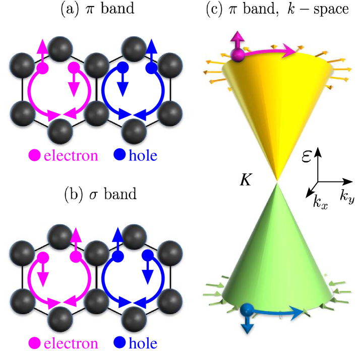
Figure 1: Illustration of the spin-valley-orbit coupling of Dirac carriers. (a) Spin ‘up’ $p_{z}$ electrons couple to counter-clockwise ($m_{l}=1$ or $\tau\sigma_{0}>0$) rotating $d$-orbitals, whereas spin ‘down’ electrons couple to clockwise rotating ones (magenta). The converse occurs for the carriers in the valence band or holes (blue). (b) Spin ‘up’ (‘down’) $p_{z}$ electrons couple to (counter)-clockwise in-plane rotating $\sigma$-orbitals, whereas spin ‘down’ (‘up’) holes couple to (counter)-clockwise in-plane $p$-orbitals of the $\sigma$ band. (c) Illustration of the CPT symmetry near the Dirac point: a left-handed quasiparticle with positive energy (magenta) is related to a right-handed one with negative energy (blue). The yellow (green) arrows indicate the sublattice spin direction along the iso-energetic paths.

Figure 1(a) illustrates, in essence, the spin-valley-orbit coupling for the low-lying energy bands showing charge-conjugation, parity, time-reversal (CPT) symmetry. The conduction or electron band (CB) is characterized by $\langle\tau s_{z}\sigma_{z}\rangle>0$. That is, a spin- “up”(-“down”) electron has $\tau\sigma_{z}>0$ ($\tau\sigma_{z}<0$), and hence, acquires a positive (negative) correction to the angular momentum (21), meaning a coupling to a counter-clockwise (clockwise) rotating $d$ orbital. That is, the $z$ component of the spin is aligned with the angular momentum correction. For the valence or hole band (VB), however, the converse occurs: having $\tau s_{z}\sigma_{z}=-1$, the spin anti-aligns with the angular momentum correction. The system is is thus CPT symmetric: For any left-handed electron state with positive energy $\varepsilon_{+}$, a corresponding conjugated right-handed hole state with energy $\varepsilon_{-}=-\varepsilon_{+}$ and opposite angular momentum can be found. The CPT symmetry and, ultimately, the chirality of Dirac electrons, is reflected in the proportionality to $\tau\sigma_{z}^{0}$ of the angular momentum corrections [see Fig. 1(c)].

II.3 The hybridized $\sigma$ bands

We consider next the hybridization of the $\sigma$ bands near the DPs. Once again, we employ the two-center Slater-Koster approximation for an $s$-orbital with $p_{x,y}$ on its NN, at $\vec{k}=\tau\vec{K}+\vec{q}$. Employing the angular momentum representation, $|l,m_{l}\rangle$, and noting that $|p_{x}\rangle\pm i|p_{y}\rangle=\sqrt{2}|1\mp 1\rangle$, the hybridized doublets (see Appendix D) are:

$$|\phi^{+}_{AB}\rangle = i\tau\cos{\gamma}|s^{A}\rangle+\sin{\gamma}|1\tau\rangle^{B},$$

$$|\phi^{+}_{BA}\rangle = i\tau\cos{\gamma}|s^{B}\rangle+\sin{\gamma}|1-\tau\rangle^{A}$$

$$|\phi^{-}_{AB}\rangle = -i\tau\sin{\gamma}|s^{A}\rangle+\cos{\gamma}|1\tau\rangle^{B},$$

$$|\phi^{-}_{BA}\rangle = -i\tau\sin{\gamma}|s^{B}\rangle+\cos{\gamma}|1-\tau\rangle^{A},$$

$$|\phi^{0}_{AB}\rangle = |1-\tau\rangle^{B},\quad|\phi^{0}_{BA}\rangle=|1\tau\rangle^{A},$$ (23)

with corresponding eigenenergies:

$$\varepsilon_{\sigma}^{\pm}=\frac{\varepsilon_{s}}{2}\pm\sqrt{\frac{\varepsilon_{s}^{2}}{4}+\frac{9V_{sp\sigma}^{2}}{2}},\ \varepsilon_{0}=0.$$

Figure 2 illustrates the hybridization of the bands at $K$ point, obtained from a 12-bands tight-binding model. The size of the symbols reflects the contribution of the orbitals to the corresponding eigenstates, whereas the colors represent the different orbitals considered in the model: $s$, $p_{x,y}$, $p_{z}$, and $d_{xz,yz}$. Note that the splittings due to SOC are not visible at this energy scales.

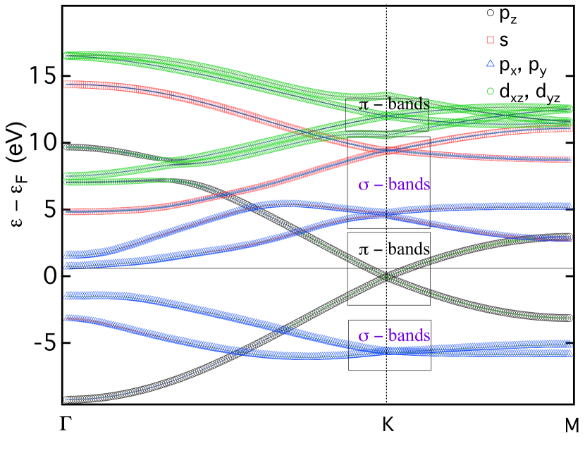
Figure 2: (Color online) Calculated bands structure of graphene obtained from a tight-binding model. The squares indicate the different hybridizations near the $K$ point, for $\sigma$ or $\pi$ bands.

The $p_{z}$ orbitals described in (3) can mix with the $\sigma$ bands either intrinsically via atomic spin-orbit interaction or extrinsically, via, e.g. Bychkov-Rashba effect Konschuh et al. (2010); Min et al. (2006); Yao et al. (2007); Rashba (2009); Gmitra et al. (2009); Huertas-Hernando et al. (2006); Kochan et al. (2017). The latter is linear in uniaxial field, and leads to the Stark effect, consisting of an atomic dipole moment induced by a perpendicular effective field, $\vec{E}=E\vec{u_{z}}$. Microscopically, the induced dipole results in a non-zero intra-atomic coupling between the $p_{z}$- and $s$ orbitals. The intrinsic SOC, on the other hand, couples the $p_{z}$-orbitals of the $\pi$ bands with the $p_{x,y}$-orbitals of the $\sigma$ bands.

The $\sigma$ band mixing near the Fermi energy is expected to be smaller than the $d$ band contribution, since the spin-orbit coupling parameter and the Stark parameter $\lambda_{z}=eE\langle s|\hat{z}|p_{z}\rangle$ are small compared to the $p$-$d$ coupling, $\lambda_{\rm soc}^{p},\lambda_{z}\ll V_{pd\pi}$. We thus consider the $\sigma$ band mixing perturbatively in the following.

II.3.1 Atomic SOC of $\sigma$ and $\pi$ bands

We consider next the atomic SOC that mixes the $p$ orbitals, hence, coupling the $\pi$ and $\sigma$ bands:

$$\hat{H}_{\rm{SOC}}=i\lambda^{p}_{\rm{soc}}\sum_{\alpha=A,B}\epsilon_{ijk}\hat{s}_{k}|p_{i}^{\alpha}\rangle\langle p_{j}^{\alpha}|+\rm{h.c.},$$

where $\lambda_{\rm{soc}}^{p}$ is the spin-orbit coupling parameter for the $p$ orbitals and $\hat{s}_{k}$ is the $k$-Pauli matrix, acting on the spin degree of freedom. The action of $\hat{H}_{\rm{SOC}}$ over the $p_{z}^{\alpha}$ orbitals ($\alpha=A,B$) is,

$$\hat{H}_{\rm{SOC}}|p_{z}^{\alpha}\rangle\otimes|s_{z}\rangle=\lambda^{p}_{\rm{soc}}\sqrt{2}s_{z}|\overline{1-s_{z}}\rangle^{\alpha},$$

where the bar over the eigenstate ($\overline{\phi}$) indicates opposite spin. The fist order correction to the $\pi$ orbitals of Eq. (3) is then:

$$|\varphi^{(1)}_{\rm AT}\rangle = \sum_{s,i}\frac{\langle\phi^{s}_{i}|\hat{H}_{\rm{SOC}}|\varphi^{0}\rangle}{\varepsilon_{\sigma}^{s}}|\phi^{s}_{i}\rangle$$

$$= -\sqrt{2}c_{A}\hat{s}_{z}\lambda^{p}_{\rm{soc}}\delta_{s_{z},-\tau}\left[\frac{\sin{\gamma}}{\varepsilon^{+}_{\sigma}}|\overline{\phi}^{+}_{BA}\rangle+\frac{\cos{\gamma}}{\varepsilon^{-}_{\sigma}}|\overline{\phi}^{-}_{BA}\rangle\right]$$

$$-\sqrt{2}c_{B}\hat{s}_{z}\lambda^{p}_{\rm{soc}}\delta_{s_{z},\tau}\left[\frac{\sin{\gamma}}{\varepsilon^{+}_{\sigma}}|\overline{\phi}^{+}_{AB}\rangle+\frac{\cos{\gamma}}{\varepsilon^{-}_{\sigma}}|\overline{\phi}^{-}_{AB}\rangle\right].$$

Projecting over the terms that yield finite angular momentum correction, we obtain:

$$\mathcal{\hat{P}}|\varphi^{(1)}_{\rm AT}\rangle=\tau\alpha_{\rm AT}\left(c_{A}|\overline{1-\tau}\rangle^{A}-c_{B}|\overline{1\tau}\rangle^{B}\right),$$ (24)

with $\mathcal{\hat{P}}=|11\rangle\langle 11|+|1-1\rangle\langle 1-1|$ and we have defined the $\sigma$-band mixing coefficient,

$$\alpha_{\rm AT}\equiv\sqrt{2}\lambda_{\rm soc}^{p}\left(\frac{\sin^{2}{\gamma}}{\varepsilon^{+}_{\sigma}}+\frac{\cos^{2}{\gamma}}{\varepsilon^{-}_{\sigma}}\right).$$

Formally, the correction given above is similar to that of (21), accounting for the chirality of the Dirac electrons. Employing the same arguments as in Sec. II.2 to Eq. (24), we conclude that spin-up electrons in the CB couple to a clockwise rotating $\sigma$ orbital, and the converse for spin-down electrons. CPT symmetry ensures that spin-down (-up) holes couple to (counter)-clockwise orbitals [see Fig. 1(b)].

II.3.2 Bychkov-Rashba SOC of $\pi$- and $\sigma$-bands

We can express the Bychkov-Rashba Hamiltonian microscopically as the coupling of the $p_{z}$ and $s$ orbitals,

$$\hat{H}_{\rm{BR}}=\lambda_{z}\hat{\vec{L}}\hat{\vec{s}}\sum_{\alpha=A,B}|s^{\alpha}\rangle\langle p_{z}^{\alpha}|+\rm{H.c.}$$

Since $\lambda_{z}$ is a very small energy scale, we can safely consider it small with respect to $\varepsilon_{\pm}$, and treat it perturbatively. The fist-order correction to the $\pi$ orbitals of Eq. (3) is then:

$$|\varphi^{(1)}_{\rm BR}\rangle = -i\lambda_{z}\tau c^{A}\hat{\vec{L}}\hat{\vec{s}}\left(\frac{\cos{\gamma}}{\varepsilon_{\sigma}^{+}}|\phi_{AB}^{+}\rangle-\frac{\sin{\gamma}}{\varepsilon_{\sigma}^{-}}|\phi_{AB}^{-}\rangle\right)$$

$$- i\lambda_{z}\tau c^{B}\hat{\vec{L}}\hat{\vec{s}}\left(\frac{\cos{\gamma}}{\varepsilon_{\sigma}^{+}}|\phi_{BA}^{+}\rangle-\frac{\sin{\gamma}}{\varepsilon_{\sigma}^{-}}|\phi_{BA}^{-}\rangle\right).$$

Using $\hat{\vec{L}}\hat{\vec{s}}=(\hat{L}_{+}\hat{s}_{+}+\hat{L}_{-}\hat{s}_{+})/2+\hat{L}_{z}\hat{s}_{z}$ and that $(\hat{L}_{+}\hat{s}_{+}+\hat{L}_{-}\hat{s}_{+})|1\pm\tau\rangle^{\alpha}=2\delta_{s_{z}\mp\tau}|p_{z}^{\alpha}\rangle$, projecting onto the states with finite $m_{l}$, we obtain:

$$\mathcal{\hat{P}}|\varphi^{(1)}_{\rm BR}\rangle=-i\alpha_{\rm BR}\tau\left(c_{A}|1\tau\rangle^{B}\delta_{s_{z},-\tau}+c_{B}|1-\tau\rangle^{A}\delta_{s_{z},\tau}\right),$$ (25)

where we have defined:

$$\alpha_{\rm BR}\equiv\lambda_{z}\left(\frac{1}{\varepsilon_{\sigma}^{-}}-\frac{1}{\varepsilon_{\sigma}^{+}}\right)\sin{\gamma}\cos{\gamma}=\frac{\sqrt{2}\lambda_{z}}{3V_{sp\sigma}}.$$

II.3.3 Principal Plane Asymmetry Spin-Orbit Coupling

We consider, for completeness, a general spin-flipping next-NN SOC related to the absence of horizontal reflection Robinson et al. (2008); Liu et al. (2011). Although there is no terminological consensus, we adopt the acronym PIA, which can be used for pseudospin-inversion asymmetry Gmitra et al. (2013) or more generally, for principal plane mirror asymmetry Gmitra et al. (2013). This term can be associated to the presence of ripples, defects or adsorbates, and it allows for a momentum-dependent coupling of the $p_{z}^{\alpha}$ and $p_{x,y}^{\beta}$-orbitals, hence, allowing coupling between the $\pi$ and $\sigma$ bands. The orbital part of the coupling takes the general form $i\tau\beta$, with $\beta=3n^{B}(V_{pp\sigma}-V_{pp\pi})/4$ real, as detailed in Appendix E:

$$\hat{H}_{\rm PIA}=i\tau\beta\left(|1\tau\rangle^{B}\langle p_{z}^{A}|\delta_{s_{z},\tau}+|1-\tau\rangle^{A}\langle p_{z}^{B}|\delta_{s_{z},-\tau}\right)+{\rm H.c.}$$

Near the DPs, we employ perturbation theory and obtain the correction due to PIA SOC:

$$|\varphi^{(1)}_{\rm PIA}\rangle = \sum_{s,i}\frac{\langle\phi^{s}_{i}|\hat{H}_{\rm{SOC}}|\varphi^{0}\rangle}{\varepsilon_{\sigma}^{s}}|\phi^{s}_{i}\rangle$$

$$= -i\tau\beta c_{A}\delta_{s_{z},\tau}\left[\frac{\sin{\gamma}}{\varepsilon_{\sigma}^{+}}|\phi_{AB}^{+}\rangle+\frac{\cos{\gamma}}{\varepsilon^{-}_{\sigma}}|\phi^{-}_{AB}\rangle\right]$$

$$-i\tau\beta c_{B}\delta_{s_{z},-\tau}\left[\frac{\sin{\gamma}}{\varepsilon_{\sigma}^{+}}|\phi_{BA}^{+}\rangle+\frac{\cos{\gamma}}{\varepsilon^{-}_{\sigma}}|\phi^{-}_{BA}\rangle\right],$$

which results, projecting over the relevant terms, on a first order correction similar to that of Bychkov-Rashba (25), only differing in the prefactor,

$$\hat{\mathcal{P}}|\varphi^{(1)}_{\rm PIA}\rangle=i\tau\alpha_{\rm PIA}\left(c_{A}|1\tau^{B}\rangle\delta_{s_{z},\tau}+c_{B}|1-\tau^{A}\rangle\delta_{s_{z},-\tau}\right),$$ (26)

with:

$$\alpha_{\rm PIA}=\frac{3n^{B}(V_{pp\sigma}-V_{pp\pi})}{4}\left(\frac{\sin^{2}{\gamma}}{\varepsilon_{\sigma}^{+}}+\frac{\cos^{2}{\gamma}}{\varepsilon_{\sigma}^{-}}\right).$$ (27)

II.4 Angular momentum contribution of the $\sigma$ band

We first evaluate the in-plane corrections $\langle L_{x,y}\rangle_{\sigma}$, taking into account the first-order corrections due to atomic SOC given in (24). Using that $\sqrt{2}\hat{L}_{x}|1,\pm\tau\rangle^{\alpha}=|p_{z}^{\alpha}\rangle$ and $\sqrt{2}\hat{L}_{y}|1,\pm\tau\rangle^{\alpha}=\pm i\tau|p_{z}^{\alpha}\rangle$, we notice that the only surviving first-order correction is along the zigzag direction:

$$\langle\hat{L}_{x}\rangle_{\rm AT} = 2{\rm Re}{\overline{\langle\varphi_{\pm}^{(0)}|\hat{L}_{x}|\varphi_{\rm AT}^{(1)}\rangle}}=\pm 2\sqrt{2}\alpha_{\rm AT}\tau\sigma_{z}^{0},$$

$$\langle\hat{L}_{y}\rangle_{\rm AT} = 0,$$ (28)

where the overbar indicates that we have averaged over spin states. This in-plane anisotropy is due to the geometry of the lattice, with a propagating $p_{x}$ orbital mode at the DPs. Recall that $p_{x}$ orbitals have a finite-$L_{x}$ contribution. The Bychkov-Rashba correction (25) and the PIA correction yield similar contributions:

$$\left(\begin{array}[]{c}\langle\hat{L}_{x}\rangle_{\rm BR}\\ \langle\hat{L}_{y}\rangle_{\rm BR}\end{array}\right)=\mp 2\sqrt{2}s_{z}\alpha_{\rm BR}\left(\begin{array}[]{c}-\sin{\varphi_{q}}\\ \cos{\varphi_{q}}\end{array}\right).$$ (33)

where we have used $\langle\hat{L}_{\alpha}\rangle_{\rm BR}=2{\rm Re}{\{\langle\varphi_{\pm}^{(0)}|\hat{L}_{\alpha}|\varphi_{\rm BR}^{(1)}\rangle\}}$, and likewise, we obtain:

$$\left(\begin{array}[]{c}\langle\hat{L}_{x}\rangle_{\rm PIA}\\ \langle\hat{L}_{y}\rangle_{\rm PIA}\end{array}\right)=\mp 2\sqrt{2}\tau s_{z}\alpha_{\rm PIA}\left(\begin{array}[]{c}-\sin{\varphi_{q}}\\ \cos{\varphi_{q}}\end{array}\right).$$ (38)

We note that the Rashba and PIA terms break parity symmetry and, as a consequence, the corrections in Eqs. (33) and (38) resemble the pseudomomentum and pseudotorque defined in (13) and (14), respectively.

We now consider the axial correction due to $\sigma$-band mixing, $\langle\hat{L}_{z}\rangle_{\sigma}$. Equations (24), (25), and (26) yield three different second-order contributions, which result into three terms proportional to $\tau\langle\sigma_{z}\rangle$, owing to the SL symmetry breaking,

$$\langle\hat{L}_{z}\rangle_{\sigma}\simeq\left((\alpha_{\rm BR}+\alpha_{\rm PIA})^{2}\ -\alpha_{\rm AT}^{2}\right)\tau\sigma_{z}^{0},$$

where the negative sign in front of the intrinsic SOC term indicates that spin-up (-down) electrons couple to (anti)-clockwise rotating $p$ orbitals within the $\sigma$ band, and the converse for the holes [see Fig. 1(b)].

For completeness, we evaluate higher-order corrections along the armchair direction, $y$. Involved calculations yield third-order corrections, (see Appendix F):

$$\langle\hat{L}_{y}\rangle_{\sigma}\simeq\alpha_{\rm AT}^{2}\alpha_{\rm BR}\left(\langle\hat{\vec{\sigma}}_{\tau}\hat{\vec{s}}\rangle+\tau\sigma_{z}^{0}\langle\hat{s}_{y}\rangle\right)+\alpha_{\rm AT}^{3}\tau\langle\hat{s}_{y}\rangle.$$ (39)

In presence of inversion symmetry, $\alpha_{\rm BR}=\alpha_{\rm PIA}=0$, the corrections along the armchair direction would only appear to third order, reflecting the intrinsic peculiarities of the lattice structure.

We have thus encountered striking anisotropies in the angular momentum corrections, which are first order along $\hat{x}$, second order along $\hat{z}$, and third order or higher along the armchair direction. Taking into account the correction of the $\pi$ bands given in (22), we can summarize our result as:

$$\langle\hat{L}_{x}\rangle \simeq \pm 2\sqrt{2}[\alpha_{\rm AT}\tau\sigma_{z}^{0}+(\alpha_{\rm PIA}+\alpha_{\rm BR})s_{z}\tau\sin{\varphi_{q}}],$$

$$\langle\hat{L}_{y}\rangle \simeq \mp 2\sqrt{2}(\alpha_{\rm PIA}+\alpha_{\rm BR})s_{z}\tau\cos{\varphi_{q}},$$

$$\langle\hat{L}_{z}\rangle \simeq \left[\frac{\lambda_{I}}{\lambda_{\rm soc}^{d}}-\alpha_{\rm AT}^{2}+(\alpha_{\rm BR}+\alpha_{\rm PIA})^{2}\right]\tau\sigma_{z}^{0}.$$ (40)

Although in an ideal, single-particle picture $\langle\tau\sigma_{z}^{0}\rangle=0$ and $\langle\tau s_{z}^{0}\rangle=0$ symmetry breaking terms would allow to resolve inherent internal structure of the Dirac carriers. For instance, electron-spin resonance on a graphene-doped sample would allow to address directly the angular momentum correction. Since the value of the gap is known, $2\lambda_{I}\simeq 42$ $\mu$eVSichau et al. (2019); Banszerus et al. (2020), resolving the $g$ tensor along the main crystallographic directions could be employed to find the value of atomic SOC, $\lambda_{\rm soc}^{p,d}$ Prada et al. (2020) or the magnitude of the Stark parameter, $\lambda_{z}$.

III Conclusions

We have considered a Dirac Hamiltonian in graphene with a mass term and we have obtained the finite angular momentum corrections along the main crystallographic axis. Intrinsic SOC causes the positive-energy carriers (electrons) in one SL with spin ‘up’ to couple to anti-clockwise rotating orbitals, whereas those with spin ‘down’ couple to clockwise rotating orbitals, with the converse occurring for negative-energy quasiparticles (holes). This confirms the CPT symmetry in the Hamiltonian, and, ultimately, reflects the chirality of the Dirac electrons. We have developed an intuitive connection between angular momentum and SL spin, where the axial quantization is given in terms of the sum of usual $L_{z}$ operator and $\nu\sigma_{z}$, with $\nu$ being the winding number. This connection is very important when establishing the selection rules that dictate how Dirac carriers couple to other carrying angular momentum quasiparticles, such as photons. Corrections to the in-plane momentum are related to a pseudovector whose torque is perpendicular to the in-plane SL spin. In the absence of external SOC, we find first-order corrections along the zigzag direction, owing to the propagating $p_{x}$ orbitals at DPs, whereas no corrections are observed in the armchair direction (up to third order). Whereas the intrinsic correction is associated with the pseudoscalar $\tau\sigma_{z}$, the extrinsic correction is related to an in-plane pseudovector perpendicular to in-plane SL spin $\sigma_{\parallel}^{\tau}$. The angular momentum correction anisotropy presented here has been confirmed in recent angle-resolved electron-spin resonance experiments Prada et al. (2020).

Acknowledgements: We acknowledge support by the Bundesminsterium für Forschung und Technologie (BMBF) through the ‘Forschungslabor Mikroelectronik Deutschland (ForLab)’. We thank L. Tiemann, R. H. Blick and T. Schmirander for fruitful discussions.

Appendix A $\hat{\vec{\sigma}}_{\tau}^{\parallel}$ is not a pseudovector

A pseudovector or axial vector transforms like a polar vector under rotations, but gains a sign flip under improper rotations, such as parity inversion. Here, we show that $\hat{\vec{\sigma}}_{\tau}\equiv(\tau\hat{\sigma}_{x},\hat{\sigma}_{y},\hat{\sigma}_{z})$ transforms as a polar vector, in spite of being expressed in terms of the Pauli matrices.

Under inversion symmetry, $\mathcal{P}$, the sublattices $A$ and $B$ are switched, as well as the valleys, and hence, the Pauli matrices transform as $\mathcal{P}\mathrel{\mathop{\mathchar 58\relax}}(\hat{\sigma}_{x},\hat{\sigma}_{y},\hat{\sigma}_{z})\to(\hat{\sigma}_{x},-\hat{\sigma}_{y},-\hat{\sigma}_{z}).$ Noting that the valleys are also switched, $\mathcal{P}\tau=-\tau$, we obtain:

$$\mathcal{\hat{P}}\hat{\vec{\sigma}}_{\tau}=(-\tau\hat{\sigma}_{x},-\hat{\sigma}_{y},-\hat{\sigma}_{z}).$$

We conclude that $\hat{\vec{\sigma}}_{\tau}$ is a polar vector, as well as the in-plane component, $\hat{\vec{\sigma}}_{\tau}^{\parallel}$.

Hence, the first term of Eq. (1) is a scalar: it is straight forward to see that it is invariant under parity, as both $\vec{q}$ and $\vec{\sigma}_{\tau}$ change sign under inversion transformation. The Semenov term, $\varepsilon_{AB}\sigma_{z}$ is, however, a pseudoscalar, as opposed to the parity-preserving Kane-Mele term, $\lambda_{I}\tau\hat{s}_{z}\hat{\sigma}_{z}$.

It is tempting to express the Hamiltonian of Eq. (1) as a scalar product of $\hat{\vec{\sigma}}_{\tau}=(\tau\sigma_{x},\sigma_{y},\sigma_{z})$ and $\hat{\vec{q}}_{\rm 3d}=(q_{x},q_{y},\hat{\lambda}/\hbar v_{F})$ by identifying $\hat{q}_{z}=\hat{\lambda}/\hbar v_{F}$. However, $\hat{\vec{q}}_{\rm 3d}$ is neither a polar nor an axial vector, and the third component can not be associated with a momentum, leading to unphysical interpretations.

Appendix B Constant of motion in Dirac Hamiltonians

In the search for a generalization of Eq. (12) in other Dirac Hamiltonians, we focus on bilayer graphene. As MacCann et al. demonstrated, McCann and Fal’ko (2006) quasiparticles in bilayer graphene can be described by using the effective Hamiltonian,

$$\hat{H}_{\rm BG}=-\tau\frac{\hbar^{2}q^{2}}{2m^{*}}\vec{\sigma}_{\tau}^{\parallel}\vec{n},\quad\vec{n}=(\cos{2\varphi_{q},\sin{2\varphi_{q}}})$$

where the resulting eigenstates gain a phase shift of $2\pi$ under an adiabatic rotation of a closed contour in momentum space, corresponding to a Berry phase of 2$\pi$ Novoselov et al. (2006) (or a winding number $\nu=2$). The time evolution of $\hat{\sigma}_{z}$ reads as:

$$\frac{{\rm d}\hat{\sigma}_{z}}{{\rm d}t} = \frac{-i\tau\hbar q^{2}}{2m^{*}}\left\{\left[\tau\hat{\sigma}_{x}\cos{2\varphi_{q}}+\hat{\sigma}_{y}\sin{2\varphi_{q}},\hat{\sigma}_{z}\right]\right\}$$ (41)

$$= \frac{\tau\hbar q^{2}}{m^{*}}\left(\tau\hat{\sigma}_{y}\cos{2\varphi_{q}}-\hat{\sigma}_{x}\sin{2\varphi_{q}}\right),$$

and likewise, we have for $\hat{L}_{z}$:

$$\frac{{\rm d}\hat{L}_{z}}{{\rm d}t} = \frac{-i\tau\hbar^{2}}{2m^{*}}\left\{\left[\tau\hat{\sigma}_{x}(\hat{q}_{x}^{2}-\hat{q}_{y}^{2})+2\hat{\sigma}_{y}\hat{q}_{x}\hat{q}_{y},\hat{x}\hat{q}_{y}-\hat{y}\hat{q}_{z}\right]\right\}$$ (42)

$$= \frac{\tau\hbar^{2}q^{2}}{m^{*}}\left(\tau\hat{\sigma}_{x}\sin{2\varphi_{q}}-\hat{\sigma}_{y}\cos{2\varphi_{q}}\right)=-\hbar\tau\dot{\sigma}_{z},$$

which is, combining (B1) and (B2),

$$\frac{{\rm d}}{{\rm d}t}(L_{z}+\hbar\tau\sigma_{z})=0,$$

resulting in (12) for $\nu=2$.

Appendix C The hybridized $\pi$-bands

We consider the unperturbed eigenstates in terms of $p_{z}$ orbitals (3). Using perturbation theory within the two-center Slater-Koster approximation Slater and Koster (1954) we obtain the non-zero $d$-orbital contribution,

$$|\varphi^{(1)}_{d}\rangle \simeq -\frac{c_{A}}{\varepsilon_{pd}}\left(V_{xz,z}^{BA}(k)|d_{xz}^{B}\rangle+V_{yz,z}^{BA}(k)|d_{yz}^{B}\rangle\right)$$

$$-\frac{c_{B}}{\varepsilon_{pd}}\left(V_{xz,z}^{AB}(k)|d_{xz}^{A}\rangle+V_{yz,z}^{AB}(k)|d_{yz}^{A}\rangle\right).$$

The matrix elements $V_{iz,z}^{\alpha\beta}(k)\equiv\sum_{i}\langle d_{xz}^{\alpha}|\hat{V}|p_{z}^{\beta}\rangle\exp{(i\vec{k}\vec{d}_{i})}$ are to be evaluated near the DPs, i.e., at $\vec{k}=\vec{q}+\vec{K}^{(\prime)}$, with $\vec{K}=-\vec{K}^{\prime}=(4\pi/3\sqrt{3}a,0)$, and $a$ being the distance between two NN ${}^{1}2$C atoms:

$$(k_{x},k_{y})=\left(\frac{4\pi\tau}{3\sqrt{3}a}+q_{x},q_{y}\right).$$

The $p$-$d$ hopping is described in terms of the NN directive cosines, $\vec{d}_{i}=(l_{i},m_{i})$ as depicted in Fig. 3. Those are $\vec{d}_{1,2}=(\pm\sqrt{3}/2,-1/2)$ and $\vec{d}_{3}=(0,1)$, giving, e.g., for the coupling of $d_{yz}^{B}$ and NN $p_{z}^{A}$ orbitals:

$$V_{xz,z}^{BA}(k) = V_{pd\pi}\sum_{i}l_{i}e^{i\vec{k}\vec{d}_{i}}$$ (43)

$$= \frac{\sqrt{3}}{2}V_{pd\pi}\left(e^{ik_{x}m_{1}}-e^{ik_{x}m_{2}}\right)e^{-i\frac{q_{y}a}{2}}$$

$$= i\sqrt{3}V_{pd\pi}e^{-i\frac{q_{y}a}{2}}\sin{\left(\frac{2\pi\tau}{3}+q_{x}a\frac{\sqrt{3}}{2}\right)}$$

$$\simeq i\tau\frac{{3V_{pd\pi}}}{2}\left(1-\frac{aq}{2}e^{i\tau\varphi_{q}}\right),$$

where we have used that $V_{xz,z}=lV_{pd\pi}$.

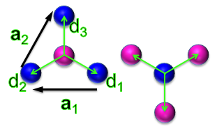
Figure 3: $A$ (blue) and $B$ (magenta) sublattices, with the NNs directive cosines, $\vec{d}_{1,2}^{BA}=-\vec{d}_{1,2}^{AB}=(\pm\sqrt{3}/2,-1/2)$ and $\vec{d}_{3}^{AB}-\vec{d}_{3}^{BA}=(0,1)$ and the primitive vectors, $\vec{a}_{1,2}$.

Likewise, we have:

$$V_{yz,z}^{BA}(k) = V_{pd\pi}\sum_{i}m_{i}e^{i\vec{k}\vec{d}_{i}}$$ (44)

$$= V_{pd\pi}\left(\frac{-1}{2}\left(e^{ik_{x}\sqrt{3}/2}+e^{-ik_{x}\sqrt{3}/2}\right)e^{-i\frac{q_{y}}{2}}+e^{iq_{y}}\right)$$

$$\simeq \frac{{3V_{pd\pi}}}{2}\left(1+\frac{aq}{2}e^{i\tau\varphi_{q}}\right).$$

It is worth noting that under sublattice swap, the matrix elements change sign, that is, $V_{iz,z}^{\alpha\beta}(k)=\sum_{i}V_{iz,z}^{\alpha\beta}e^{i(k_{x}l_{i}+k_{y}m_{i})}=-\sum_{i}V_{iz,z}^{\beta\alpha}e^{-i(k_{x}l_{i}+k_{y}m_{i})}$, since the directive cosines change sign (see Fig. 3):

$$V_{iz,z}^{AB}(k)=-[V_{iz,z}^{BA}(k)]^{*}=-V_{z,iz}^{AB}(k).$$

This has important consequences, implying that the topological character of the $\pi$ bands is preserved. To lowest order, that is, neglecting the linear in momentum terms, we obtain:

$$|\varphi^{(1)}_{d}\rangle \simeq -\frac{3V_{pd\pi}}{2\varepsilon_{pd}}\left[c_{A}\left(|d_{yz}^{B}\rangle+i\tau|d_{xz}^{B}\rangle\right)\right.$$

$$\left.+c_{B}\left(-|d_{yz}^{A}\rangle+i\tau|d_{xz}^{A}\rangle\right)\right]$$

$$= -\frac{3i\tau V_{pd\pi}}{\sqrt{2}\varepsilon_{pd}}\left(c_{A}|2\tau\rangle^{B}+c_{B}|2-\tau\rangle^{A}\right),$$

where in the last step we have used the angular momentum representation, $|l,m_{l}\rangle$, with $l=2$, and

$$|2\pm 1\rangle=\frac{1}{\sqrt{2}}\left(|d_{xz}\rangle\pm i|d_{yz}\rangle\right).$$

Appendix D The hybridized $\sigma$ bands near DPs

We consider the $sp^{2}$ hybridization via $\sigma$ bonds near the DPs. The low-energy Hamiltonian can be evaluated within a reduced Hilbert space spanned by $\{s^{\alpha},p_{x}^{\beta},p_{y}^{\beta}\}$, $\alpha\neq\beta$, as dominant hopping within the $\sigma$ band occurs between NN $s$- and $p_{x,y}$-orbitals Min et al. (2006). The hoppings between an $s$-orbital in SL $A$ and $p_{x}$ ($p_{y}$) in the SL $B$ is given by $l_{i}V_{sp\sigma}$ ($m_{i}V_{sp\sigma}$). Hence, we can employ the results of the previous section, where only the prefactor changes. Using Eq. (43), we obtain:

$$V_{s,p_{x}}^{BA}(k) \simeq V_{sp\sigma}\sum_{i}l_{i}e^{i\vec{k}\vec{d}_{i}}=i\tau\frac{{3V_{sp\sigma}}}{2}\left(1-\frac{aq}{2}e^{i\tau\varphi_{q}}\right)$$

Likewise, we have:

$$V_{s,p_{y}}^{BA}(k) \simeq \frac{3}{2}V_{sp\sigma}\left(1+\frac{a}{2}(\tau q_{x}+iq_{y})\right),$$

and it follows, using symmetry arguments, $V_{s,p_{x}}^{AB}(k)=-[V_{s,p_{x}}^{BA}(k)]*$, that is:

$$V_{s,p_{x}}^{AB}(k)\simeq\frac{3i\tau}{2}V_{sp\sigma}\left(1-\frac{a}{2}(\tau q_{x}-iq_{y})\right),$$

$$V_{s,p_{y}}^{AB}(k)\simeq-\frac{3}{2}V_{sp\sigma}\left(1+\frac{a}{2}(\tau q_{x}-iq_{y})\right).$$

In the basis spanned by $\{s^{A},|1,\tau\rangle^{B}\},|1,-\tau\rangle^{B}\}$ with $|1,\pm\tau\rangle^{B}\equiv(|p_{x}\rangle^{B}\mp i\tau|p_{y}\rangle^{B})/\sqrt{2}$, we have:

$$\hat{H}_{h}^{BA}=\left(\begin{array}[]{ccc}\varepsilon_{s}&3i\tau V_{sp\sigma}/\sqrt{2}&0\\ -3i\tau V_{sp\sigma}/\sqrt{2}&\varepsilon_{p}&0\\ 0&0&\varepsilon_{p}\end{array}\right),{\rm{}}$$ (46)

with eigenvalues:

$$\varepsilon_{\sigma}^{\pm}=\frac{\varepsilon_{s}+\varepsilon_{p}}{2}\pm\sqrt{\frac{(\varepsilon_{s}-\varepsilon_{p})^{2}}{4}+\frac{9V_{sp\sigma}^{2}}{2}},\ \varepsilon_{0}=\varepsilon_{p},$$

and corresponding eigenvectors, with $\phi^{0}_{AB}=|1-\tau\rangle^{B}$ and

$$\phi^{+}_{AB}=\left(\begin{array}[]{c}i\tau\cos{\gamma}\\ \sin{\gamma}\\ 0\end{array}\right),\quad\phi^{-}_{AB}=\left(\begin{array}[]{c}-i\tau\sin{\gamma}\\ \cos{\gamma}\\ 0\end{array}\right),$$ (47)

where we have defined

$$\gamma=\arctan{\left[\frac{3V_{sp\sigma}}{\sqrt{2}(\varepsilon_{\sigma}^{+}-\varepsilon_{p})}\right]}.$$

Likewise, we have that in the basis spanned by $\{|s\rangle^{B},|1,-\tau\rangle^{A},|1,\tau\rangle^{A}\}$, the hopping Hamiltonian is formally identical to that of Eq. (46), yielding same eigenvalues, and similar eigenvectors:

$$\phi^{+}_{BA}=\left(\begin{array}[]{c}i\tau\cos{\gamma}\\ \sin{\gamma}\\ 0\end{array}\right),\quad\phi^{-}_{BA}=\left(\begin{array}[]{c}-i\tau\sin{\gamma}\\ \cos{\gamma}\\ 0\end{array}\right),$$ (48)

with $\phi^{0}_{AB}=|1\tau\rangle^{A}$.

Appendix E PIA coupling

We consider now the coupling induced by horizontal plane mirror asymmetry, PIA. The term arises in the presence of adsorbates, Robinson et al. (2008) ripples Kochan et al. (2017); Gmitra et al. (2013) or other defects, and causes a coupling between the $p_{z}$ and the NNs $p_{x,y}$ orbitals Liu et al. (2011). We account for this term assuming a vertical relative component of one lattice with respect to the other, with a directive cosinus given by $n_{i}^{AB}=n^{B}$ $\forall$ $i$. Employing the two-center Slater-Koster approximation Slater and Koster (1954), the relevant orbital matrix elements near DPs are $V^{BA}_{\eta,z}(q)\equiv\langle p_{\eta}^{B}|\hat{V}|p_{z}^{A}\rangle$, with:

$$V^{BA}_{x,z}(q) = (V_{pp\sigma}-V_{pp\pi})\sum_{i}n_{i}l_{i}e^{i\vec{k}\vec{d}_{i}}=$$

$$= i\tau\frac{3n^{B}}{2}(V_{pp\sigma}-V_{pp\pi})\left(1-\frac{aq}{2}e^{i\tau\varphi_{q}}\right),$$

$$V^{BA}_{y,z}(q) = (V_{pp\sigma}-V_{pp\pi})\sum_{i}n_{i}m_{i}e^{i\vec{k}\vec{d}_{i}}=$$

$$= \frac{3n^{B}}{2}(V_{pp\sigma}-V_{pp\pi})\left(1+\frac{aq}{2}e^{i\tau\varphi_{q}}\right),$$

where we have employed the procedure of Eqs. (43) and (44), and $n^{B}$ is a sublattice $B$ vertical displacement. $V^{AB}_{\eta,z}(q)$ are trivially obtained, using $V^{AB}_{\eta,z}(q,n^{B})=-(V^{BA}_{\eta,z}(q,n^{A}))^{*}$. The allowed SOC term is then of the form $(\hat{L}_{+}\hat{s}_{-}+\hat{L}_{-}\hat{s}_{+})/2$, which results into the coupling of the $p_{z}$ orbitals to the $\sigma$ band is given by:

$$\frac{1}{2}\langle 1\tau|^{B}\hat{V}|p_{z}^{A}\rangle\otimes(\hat{s}_{x}+i\tau\hat{s}_{y})=i\tau\delta_{s_{z},\tau}\frac{3n^{B}}{4}(V_{pp\sigma}-V_{pp\pi}),$$

$$\frac{1}{2}\langle 1-\tau|^{A}\hat{V}|p_{z}^{B}\rangle\otimes(\hat{s}_{x}-i\tau\hat{s}_{y})=i\tau\delta_{s_{z},-\tau}\frac{3n^{A}}{4}(V_{pp\sigma}-V_{pp\pi}),$$

where the spin degree of freedom has been explicitly evaluated in terms of the valley, to ensure PT symmetry.

Appendix F Third order corrections

We consider the $\hat{H}_{\rm BR}+\hat{H}_{\rm soc}$ and calculate the corrections over $|\varphi^{(1)}_{\rm soc}\rangle$ and $|\varphi^{(1)}_{\rm BR}\rangle$, which are the second order corrections to the WF:

$$|\varphi^{(2)}\rangle \simeq \alpha_{\rm soc}^{2}\left[c_{A}\langle\tau\hat{s}_{x}+i\hat{s}_{y}\rangle^{A}|p_{z}^{A}\rangle-c_{B}\langle-\tau\hat{s}_{x}+i\hat{s}_{y}\rangle^{B}|p_{z}^{B}\rangle\right]$$

$$- i\alpha_{\rm BR}\alpha_{\rm soc}\left[c_{A}\langle-\tau\hat{s}_{x}+i\hat{s}_{y}\rangle^{B}|p_{z}^{B}\rangle+\right.$$

$$\left.c_{B}\langle\tau\hat{s}_{x}+i\hat{s}_{y}\rangle^{A}|p_{z}^{A}\rangle\right],$$

where $\langle\dots\rangle^{\alpha}$ indicates that the expectation value is to be calculated in SL $\alpha$. The next order correction to angular momentum along $y$ would be $2{\rm Re}{\left\{\langle\varphi^{(1)}_{\sigma}|\hat{L}_{y}|\varphi^{(2)}\rangle\right\}}$, yielding:

$$\langle\hat{L}_{y}\rangle \simeq \alpha_{\rm soc}^{3}\tau(\langle\hat{s}_{y}\rangle^{A}|c_{A}|^{2}+\langle\hat{s}_{y}\rangle^{B}|c_{B}|^{2})+$$ (49)

$$\alpha_{\rm soc}^{2}\alpha_{\rm BR}\left(\tau c_{A}^{*}c_{B}\langle\hat{s}_{x}\rangle^{A}+\tau c_{A}c_{B}^{*}\langle\hat{s}_{x}\rangle^{B}\right.$$

$$\left.+ic_{A}^{*}c_{B}\langle\hat{s}_{y}\rangle^{A}-ic_{A}c_{B}^{*}\langle\hat{s}_{y}\rangle^{B}\right).$$

In absence of spin-SL coupling, we can consider $\langle\hat{s}_{i}\rangle^{A}=\langle\hat{s}_{i}\rangle^{B}=\langle\hat{s}_{i}\rangle$, $i=x,y$. Using that $|c_{A}|^{2}+|c_{B}|^{2}\simeq 1$ and (3), we obtain (39).

References

- Novoselov et al. (2005) K. S. Novoselov, A. K. Geim, S. V. Morozov, D. Jiang, M. I. Katsnelson, I. V. Grigorieva, S. V. Dubonos, and A. A. Firsov, Nature 438, 197 (2005).
- Katsnelson et al. (2006) M. I. Katsnelson, K. Novoselov, and A. K. Geim, Nature Physics 2, 620 (2006).
- Geim and Novoselov (2010) A. K. Geim and K. S. Novoselov, in Nanoscience and Technology: A Collection of Reviews from Nature Journals (World Scientific, 2010) pp. 11–19.
- Nair et al. (2008) R. R. Nair, P. Blake, A. N. Grigorenko, K. S. Novoselov, T. J. Booth, T. Stauber, N. M. R. Peres, and A. K. Geim, Science 320, 1308 (2008).
- Katsnelson and Novoselov (2007) M. Katsnelson and K. Novoselov, Solid State Communications 143, 3 (2007), exploring graphene.
- Giuliani et al. (2012) A. Giuliani, V. Mastropietro, and M. Porta, Annals of Physics 327, 461 (2012).
- Marino et al. (2015) E. C. Marino, L. O. Nascimento, V. S. Alves, and C. M. Smith, Phys. Rev. X 5, 011040 (2015).
- Golub et al. (2020) A. Golub, R. Egger, C. Müller, and S. Villalba-Chávez, Phys. Rev. Lett. 124, 110403 (2020).
- Kane and Mele (2005a) C. L. Kane and E. J. Mele, Physical Review Letters 95, 226801 (2005a).
- Kane and Mele (2005b) C. L. Kane and E. J. Mele, Physical Review Letters 95, 146802 (2005b).
- Sichau et al. (2019) J. Sichau, M. Prada, T. Anlauf, T. J. Lyon, B. Bosnjak, L. Tiemann, and R. Blick, Physical Review Letters 122, 046403 (2019).
- Mecklenburg and Regan (2011) M. Mecklenburg and B. C. Regan, Phys. Rev. Lett. 106, 116803 (2011).
- Soodchomshom (2013) B. Soodchomshom, Chinese Physics Letters 30, 126201 (2013).
- Song et al. (2015) D. Song, V. Paltoglou, S. Liu, Y. Zhu, D. Gallardo, L. Tang, J. Xu, M. Ablowitz, N. K. Efremidis, and Z. Chen, Nature Comms. 6, 6272 (2015).
- Liu et al. (2018) X. Liu, D. Song, S. Xia, Z. Dai, L. Tang, J. Xu, and Z. Chen, in Conference on Lasers and Electro-Optics (Optical Society of America, 2018) p. FTh3E.4.
- Liu et al. (2020) X. Liu, S. Xia, E. Jajtić, D. Song, D. Li, L. Tang, D. Leykam, J. Xu, H. Buljan, and Z. Chen, Nature Comms. 11, 1586 (2020).
- Prada et al. (2020) M. Prada, J. Sichau, L. Tiemann, and R. Blick, unpublished (2020).
- Castro Neto et al. (2009) A. H. Castro Neto, F. Guinea, N. M. R. Peres, K. S. Novoselov, and A. K. Geim, Reviews of Modern Physics 81, 109 (2009).
- Katsnelson (2012) M. I. Katsnelson, Graphene: Carbon in Two Dimensions (Cambridge university press, 2012).
- Semenoff (1984) G. W. Semenoff, Phys. Rev. Lett. 53, 2449 (1984).
- Shapere and Wilczek (1989) A. Shapere and F. Wilczek, Geometrical Phases in Physics (Singapore, 1989).
- Ando et al. (1998) T. Ando, T. Nakanishi, and R. Saito, Journal of the Physical Society of Japan 67, 2857 (1998).
- McEuen et al. (1999) P. L. McEuen, M. Bockrath, D. H. Cobden, Y.-G. Yoon, and S. G. Louie, Phys. Rev. Lett. 83, 5098 (1999).
- Hasan and Kane (2010) M. Z. Hasan and C. L. Kane, Reviews of Modern Physics 82, 3045 (2010).
- Asbóth et al. (2006) J. K. Asbóth, L. Oroszlány, and A. Pályi, A Short Course on Topological Insulators (Springer, 2006).
- Prada et al. (2011) E. Prada, P. San-Jose, L. Brey, and H. Fertig, Solid State Communications 151, 1075 (2011).
- Konschuh et al. (2010) S. Konschuh, M. Gmitra, and J. Fabian, Physical Review B 82, 245412 (2010).
- Huertas-Hernando et al. (2006) D. Huertas-Hernando, F. Guinea, and A. Brataas, Physical Review B 74, 155426 (2006).
- Min et al. (2006) H. Min, J. E. Hill, N. A. Sinitsyn, B. R. Sahu, L. Kleinman, and A. H. MacDonald, Physical Review B 74, 165310 (2006).
- Yao et al. (2007) Y. Yao, F. Ye, X.-L. Qi, S.-C. Zhang, and Z. Fang, Physical Review B 75, 041401 (2007).
- Rashba (2009) E. I. Rashba, Physical Review B 79, 161409 (2009).
- Gmitra et al. (2009) M. Gmitra, S. Konschuh, C. Ertler, C. Ambrosch-Draxl, and J. Fabian, Physical Review B 80, 235431 (2009).
- Kochan et al. (2017) D. Kochan, S. Irmer, and J. Fabian, Phys. Rev. B 95, 165415 (2017).
- Robinson et al. (2008) J. P. Robinson, H. Schomerus, L. Oroszlány, and V. I. Fal’ko, Phys. Rev. Lett. 101, 196803 (2008).
- Liu et al. (2011) C.-C. Liu, H. Jiang, and Y. Yao, Phys. Rev. B 84, 195430 (2011).
- Gmitra et al. (2013) M. Gmitra, D. Kochan, and J. Fabian, Phys. Rev. Lett. 110, 246602 (2013).
- Banszerus et al. (2020) L. Banszerus, B. Frohn, T. Fabian, S. Somanchi, A. Epping, M. Müller, D. Neumaier, K. Watanabe, T. Taniguchi, F. Libisch, B. Beschoten, F. Hassler, and C. Stampfer, Phys. Rev. Lett. 124, 177701 (2020).
- McCann and Fal’ko (2006) E. McCann and V. I. Fal’ko, Phys. Rev. Lett. 96, 086805 (2006).
- Novoselov et al. (2006) K. S. Novoselov, E. McCann, S. V. Morozov, V. I. Fal’ko, M. I. Katsnelson, U. Zeitler, D. Jiang, F. Schedin, and A. K. Geim, Nature Physics 2, 177 (2006).
- Slater and Koster (1954) J. C. Slater and G. F. Koster, Phys. Rev. 94, 1498 (1954).