Improved Effective Dynamics of Loop-Quantum-Gravity Black Hole and Nariai Limit

Abstract

We propose a new model of the spherical symmetric quantum black hole in the reduced phase space formulation. We deparametrize gravity by coupling to the Gaussian dust which provides the material coordinates. The foliation by dust coordinates covers both the interior and exterior of the black hole. After the spherical symmetry reduction, our model is a 1+1 dimensional field theory containing infinitely many degrees of freedom. The effective dynamics of the quantum black hole is generated by an improved physical Hamiltonian ${\bf H}_{\Delta}$. The holonomy correction in ${\bf H}_{\Delta}$ is implemented by the $\bar{\mu}$-scheme regularization with a Planckian area scale $\Delta$ (which often chosen as the minimal area gap in Loop Quantum Gravity). The effective dynamics recovers the semiclassical Schwarzschild geometry at low curvature regime and resolves the black hole singularity with Planckian curvature, e.g. $R_{\mu\nu\rho\sigma}R^{\mu\nu\rho\sigma}\sim 1/{\Delta}^{2}$. Our model predicts that the evolution of the black hole at late time reaches the charged Nariai geometry ${\rm dS}_{2}\times S^{2}$ with Planckian radii $\sim\sqrt{\Delta}$. This result is similar to the earlier work of the $\bar{\mu}$-scheme black hole Bohmer:2007wi but is free of its problems. The Nariai geometry is stable under linear perturbations but may be unstable by nonperturbative quantum effects. Our model suggests the existence of quantum tunneling of the Nariai geometry and a scenario of black-hole-to-white-hole transition. During the transition, the linear perturbations exhibit chaotic dynamics with Lyapunov exponent $\lambda=2\pi T_{\rm dS}\sim\Delta^{-1/2}$ relating to the Hawking temperature $T_{\rm dS}$ of ${\rm dS}_{2}$. In addition, the Nariai geometry in our model provides an interesting example of Wheeler’s bag of gold and contains infinitely many infrared soft modes with zero energy density. These infrared modes span a Hilbert space carrying a representation of 1-dimensional spatial diffeomorphisms (or the Witt/Virasoro algebra). The spatial diffeomorphisms are conserved charges of the effective dynamics by ${\bf H}_{\Delta}$.

1 Introduction

The research on quantum black holes has recently made important progress in the framework of Loop Quantum Gravity (LQG) (see e.g. Ashtekar:2005qt ; Modesto:2005zm ; Bohmer:2007wi ; Ashtekar:2010qz ; Chiou:2012pg ; Gambini:2013hna ; Bianchi:2018mml ; DAmbrosio:2020mut ; Olmedo:2017lvt ; Ashtekar:2018cay ; Bojowald:2018xxu ; Bodendorfer:2019cyv ; Alesci:2019pbs ; Assanioussi:2019twp ; Kelly:2020lec ; Gambini:2020nsf , see also Ashtekar:2020ifw for a recent review). LQG, as a background-independent and non-perturbative approach of quantum gravity, has the advantage for studying non-perturbative quantum effects in strong gravitational fields such as inside the black hole or the beginning of the universe. In particular, LQG leads to the success of resolving both black hole and big-bang singularities (see e.g. Bojowald:2001xe ; Ashtekar:2006wn for cosmology). In both cases, the classical curvature singularities are replaced by the non-singular bounces where their curvatures are finite and Planckian.

These developments of LQG black hole are based on symmetry reduced models. Instead of the full quantum theory of gravity, these models of black hole quantize spherical symmetric gravitational degrees of freedom (DOFs). They fall into 2 categories: The models in the first category e.g. Ashtekar:2005qt ; Modesto:2005zm ; Bohmer:2007wi ; Ashtekar:2010qz ; Olmedo:2017lvt ; Ashtekar:2018cay ; Bodendorfer:2019cyv ; Assanioussi:2019twp quantizes the black hole interior and exterior separately using the homogeneous Kantowski-Sachs slices, and they only quantize a finite number of DOFs due to the spherical symmetry and homogeneity. The models in the second category e.g. Chiou:2012pg ; Gambini:2013hna ; Alesci:2019pbs ; Kelly:2020lec ; Gambini:2020nsf only reduce the DOFs by spherical symmetry, so these models are 1+1 dimensional field theories which still contain infinitely many DOFs, and they can treat both the black hole interior and exterior in a unified manner. Our approach in this work belongs to the second category.

The effective dynamics is one of important tools for studying black holes in LQG. The effective Hamiltonian of the black hole modifies the classical Hamiltonian in the canonical spherical symmetric gravity by including holonomy corrections to the Ashtekar-Barbero connection $A$, motivated by the LQG quantization. It is shown that in Loop Quantum Cosmology (LQC), the effective dynamics is able to accurately capture key features of the quantum dynamics Rovelli:2013zaa . It is expected that the effective dynamics should also be valid for black hole, or at least be a crucial first step toward understanding full quantum effects of black hole. The effective dynamics from all the existing models lead to the black hole singularity resolution and bounce, but their detailed behaviors are different and depend on their schemes of the holonomy corrections. The choice of schemes are involved in these models due to the regularization/discretization of the Hamiltonian in which the curvature of $A$ is discretized by the loop holonomy around a plaquette. Here are a few examples of schemes used in these models: Among models in the first category, the earliest models Ashtekar:2005qt ; Modesto:2005zm follow the strategy similar to the $\mu_{0}$-scheme in LQC, and use plaquettes with constant fiducial scale. Their resulting behaviors of the bounce depend on the fiducial scale of plaquette. The model in Bohmer:2007wi follows the similar strategy of the improved $\bar{\mu}$-scheme of LQC, where the scale of the plaquette is dynamical. This model removes the dependence on the fiducial scale, and interestingly relates the final state of black hole to the Nariai geometry ${\rm dS}_{2}\times S^{2}$ (see e.g. Bousso:1996pn for earlier studies of the Nariai solution). But it has two problems (1) it gives large quantum effect near the event horizon where the spacetime curvature is small (this may be the consequence from choosing the Kantowski-Sachs foliation whose spatial slice approaching null near the horizon), and (2) the area of 2-sphere becomes too small in the evolution, making the model self-inconsistent with the $\bar{\mu}$-type regularization (see Ashtekar:2018cay for the discussion). The more recent model Ashtekar:2018cay applies a new regularization scheme. In this scheme, the fiducial scale is a conserved Dirac observable and remains constant along the trajectory of evolution, but it may change value along different trajectories. The models Chiou:2012pg ; Gambini:2013hna ; Kelly:2020lec ; Gambini:2020nsf in the second category applies the $\bar{\mu}$-type regularization, complemented by certain gauge fixing and choice of lapse function. The foliations of these models are not Kantowski-Sachs but cover both the black hole interior and exterior.

In this work, we propose a new model of the spherical symmetric LQG black hole and study the effective dynamics. The model is embedded in the framework of the reduced phase formulation. We deparametrize gravity by coupling it to the Gaussian dust Kuchar:1990vy ; Giesel:2012rb . The dust fields provide a material reference frame of the time and space. The dynamics in the reduced phase space is governed by a physical Hamiltonian, which in our case is identical to the Hamiltonian constraint with unit lapse. When reducing to the sector of spherical symmetric DOFs, we obtain an 1+1 dimensional Hamiltonian field theory describing the spherical symmetric gravity-dust system. Classical solutions of this theory are Lemaitre-Tolman-Bondi spacetimes (classically, our model closely relates to the earlier spherical symmetric reduced phase space model Giesel:2009jp , see also Kelly:2020lec ; Munch:2020czs for recent works on coupling dust to black hole). We prefer the reduced phase space formulation because the dynamics is generated by the Hamiltonian which can make sense the unitarity when we pass to the quantum theory.

Our model applies the $\bar{\mu}$-scheme regularization (following Chiou:2012pg ) to include the holonomy correction to the physical Hamiltonian. The improved effective Hamiltonian ${\bf H}_{\Delta}$ depends on the Planckian area scale $\Delta\sim\ell_{P}$ which usually is set to be the minimal LQG area gap. The improved effective dynamics is given by solving the Hamiltonian equations of motion (EOMs) of ${\bf H}_{\Delta}$. The EOMs are a set of partial differential equations (PDEs) which we call the effective EOMs. The corrections of $O(\Delta)$ are understood as quantum corrections to the classical EOMs. As a reason of choosing the $\bar{\mu}$-scheme regularization, it has the nice properties that the improved effective dynamics from ${\bf H}_{\Delta}$ has infinitely many conserved charges corresponding to spatial diffeomorphisms, which play an interesting role in our discussion.

An important advantage of our model is that it includes infinitely many DOFs and describes the effective dynamics of both interior and exterior of the black hole in one set of effective EOMs. Indeed, in the case of zero dust density and classical limit $\Delta\to 0$, the solution of effective EOMs is the Schwarzschild geometry in Lemaitre coordinate, which covers both the interior and exterior of the black hole. Classically the spatial slice of Lemaitre coordinate starts from the spatial infinity, crosses the event horizon, and ends at the singularity (the slice is further extended to another infinity by the singularity resolution in our model). Our model based on the reduced phase formulation is different from other ones in the second category. ${\bf H}_{\Delta}$ corresponds to the unit lapse function, and does not use the areal gauge fixing, as other 2 differences from Gambini:2013hna ; Kelly:2020lec ; Gambini:2020nsf .

When solving the effective EOMs of ${\bf H}_{\Delta}$, we mainly focus on the situation with small dust density $\rho$. We firstly derive non-perturbatively the vacuum solution in the case of negligible $\rho$, then turn on nontrivial $\rho$ by including linear perturbations. The vacuum solution is obtained by the numerical method with high precision. Some features of this solution are highlighted below, while the details is given in Section 5.

1. The solution satisfies the semiclassical boundary condition, i.e. reduces to classical Schwarzschild geometry in Lemaitre coordinate near spatial infinity. The quantum correction are negligible in the low curvature regime.

2. The black hole singularity is resolved and replaced by the non-singular bounce of the spatial volume element. The Kretschmann scalar $\mathcal{K}\sim\Delta^{-2}$ at the bounce is Planckian as $\Delta\sim\ell_{P}^{2}$. The Lemaitre spatial slice, classically ending at the singularity, is now further extended to another infinity.

3. After the bounce, the evolution stabilizes asymptotically to the charged Nariai limit ${\rm dS}_{2}\times S^{2}$ with different dS and $S^{2}$ radii. It is interesting that we obtain the Nariai limit similar to the result in Bohmer:2007wi , although our model is very different from theirs (the model in Bohmer:2007wi belongs to the first category while ours belongs to the second category).

4. Although we have the similar result as in Bohmer:2007wi , our model is free of its problems: Thanks to the foliation used in our approach, the geometry near the event horizon is semiclassical with negligible quantum correction. The area of 2-sphere never becomes smaller than $\Delta$ in the evolution, consistent with the $\bar{\mu}$-scheme regularization.

The charged Nariai limit ${\rm dS}_{2}\times S^{2}$ in our model is due to quantum effect. Both radii of dS and $S^{2}$ are of $O(\sqrt{\Delta})$. The appearance of the Nariai geometry is an interesting feature of the model, given that extensive studies in 90s suggesting the relation between the Nariai geometry and the black hole remanent e.g. Hawking:1995ap ; Bousso:1999ms ; Bousso:1996pn ; Bousso:1996wz . As a difference from early results on the Nariai limit, in our model the Nariai geometry ${\rm dS}_{2}\times S^{2}$ is stable when we turn on linear perturbations. This result is similar to Bohmer:2007wi ; Boehmer:2008fz . But we find evidence that the Nariai geometry is unstable by taking into account the non-perturbative quantum effect. The quantum tunneling effect may send ${\rm dS}_{2}\times S^{2}$ to $\widetilde{{\rm dS}_{2}\times S^{2}}$ with opposite time orientation. Then following the effective EOMs, $\widetilde{{\rm dS}_{2}\times S^{2}}$ decays to the Schwarzschild white hole spacetime with complete future timelike and null infinities. The solution evolving from $\widetilde{{\rm dS}_{2}\times S^{2}}$ to the white hole is the time reversal of the vacuum solution discussed above. The entire picture taking into account the black hole evaporation and the quantum tunneling proposes a scenario of black-hole-to-white-hole transition similar to DAmbrosio:2020mut ; Bianchi:2018mml ; Rovelli:2014cta . The detailed discussions of the black-hole-to-white-hole transition and evidences of quantum tunneling is given in Sections 6, 7, and 8.

When we turn on linear perturbations on $\widetilde{{\rm dS}_{2}\times S^{2}}$, the perturbations exhibit chaotic dynamics where we can extract the Lyapunov exponent $\lambda=2\pi T_{\rm dS}$ relating to the Hawking temperature $T_{\rm dS}$ at the cosmological horizon of ${\rm dS}_{2}$ (see Section 9). Moreover $\lambda\sim\Delta^{-1/2}$ indicates that this chaos is due to the quantum gravity effect. The relation between $\lambda$ and $T_{\rm dS}$ resembles the known relation in the black hole butterfly effect Shenker:2013pqa ; Maldacena:2015waa .

As another interesting aspect of the Nariai limit ${\rm dS}_{2}\times S^{2}$, it is an example of Wheeler’s bag of gold (see Section 10). The foliation corresponds to the inflationary coordinate of ${\rm dS}_{2}$ and gives large space volume behind the event horizon of small area at the late time of the evaporation. When we turn on perturbations, we find that all perturbations become infinitely many infrared modes with zero energy density in ${\rm dS}_{2}\times S^{2}$. It is also the reason why ${\rm dS}_{2}\times S^{2}$ geometry is perturbatively stable. This result seems to suggests that ${\rm dS}_{2}\times S^{2}$ should have quantum degeneracy, and all the infrared modes should span a Hilbert space $\mathcal{H}_{{\rm dS}_{2}\times S^{2}}$. In the reduced phase space formulation, the spatial diffeomorphisms are the symmetries of the physical Hamiltonian ${\bf H}_{\Delta}$ and give infinitely many conserved charges. Then $\mathcal{H}_{{\rm dS}_{2}\times S^{2}}$ is the representation space of the spatial diffeomorphism group ${\rm Diff}(S^{1})$ on the space of ${\rm dS}_{2}$. The Lie algebra of ${\rm Diff}(S^{1})$ is the Witt algebra, or the Virasoro algebra if the central extension is considered.

Here is the organization of this paper: Section 2 discusses the preliminaries including the reduced phase space formulation with Gaussian dust and the spherical symmetric reduction. Section 3 constructs the improved effective Hamiltonian by the $\bar{\mu}$-scheme regularization. Section 4 discusses the effective EOMs. Section 5 discusses the numerical black hole solution of the effective EOMs and the Nariai limit. Section 6 takes into account the black hole evaporation and motivates the extension of the effective spacetime. 7 discusses the scenario of the black-hole-to-white-hole transition. 8 discusses the evidence of quantum tunneling from ${\rm dS}_{2}\times S^{2}$ to $\widetilde{{\rm dS}_{2}\times S^{2}}$. Section 9 demonstrates the chaos of perturbations on $\widetilde{{\rm dS}_{2}\times S^{2}}$. Section 10 discusses the relation between the Nariai limit and Wheeler’s bag of gold, and shows that ${\rm dS}_{2}\times S^{2}$ contains infinitely many infrared states. Section 11 discusses some future perspectives and open questions.

2 Reduced phase space formulation

2.1 Deparametrized gravity with Gaussian dust

The reduced phase space formulation couples gravity to clock fields at classical level. In this paper, we mainly focus on the scenario of gravity coupled to Gaussian dust Kuchar:1990vy ; Giesel:2012rb . The action is given by

$$S=S_{\rm GR}+S_{\rm GD},$$ (1)

where $S_{\rm GR}$ is the Host action of gravity holst

$$S_{\rm GR}\left[e^{\mu}_{I},\Omega_{\mu\nu}^{IJ}\right]=\frac{1}{16\pi G}\int_{M}d^{4}y\,\sqrt{|\operatorname{det}(g)|}\,e_{I}^{\mu}e_{J}^{\nu}\left(\Omega_{\mu\nu}^{IJ}+\frac{1}{2\beta}\epsilon_{\ \ \ KL}^{IJ}\Omega_{\mu\nu}^{KL}\right)$$ (2)

where the tetrad $e^{\mu}_{I}$ determines the 4-metric by $g_{\mu\nu}=\eta_{IJ}e^{\mu}_{I}e^{\nu}_{J}$, and $\Omega_{\mu\nu}^{IJ}$ is the curvature of the so(1,3) connection $\omega_{\mu}^{IJ}$. $\beta$ is the Barbero-Immirzi parameter. $S_{\rm GD}$ is the action of the Gaussian dust:

$$S_{\rm GD}\left[\rho,g_{\mu\nu},T,S^{j},W_{j}\right]=-\int_{M}\mathrm{d}^{4}y\sqrt{|\operatorname{det}(g)|}\left[\frac{\rho}{2}\left(g^{\mu\nu}\partial_{\mu}T\partial_{\nu}T+1\right)+g^{\mu\nu}\partial_{\mu}T\left(W_{j}\partial_{\nu}S^{j}\right)\right]$$ (3)

where $T,S^{j=1,2,3}$ are clock fields and defines time and space coordinates in the dust reference frame. $\rho,W_{j}$ are Lagrange multipliers. The energy-momentum tensor of the Gaussian dust is

$$T_{\mu\nu}=\rho U_{\mu}U_{\nu}-U_{(\mu}W_{\nu)},\quad U_{\mu}=-\partial_{\mu}T,\quad W_{\nu}=W_{j}\partial_{\nu}S^{j}.$$ (4)

which indicates that $\rho$ is the energy density and $W_{\mu}$ relates to the heat-flow Kuchar:1990vy .

We assume $M\simeq\mathbb{R}\times\Sigma$ and and make Legendre transform of dust variables:

$$\begin{aligned} P&:=\frac{\delta{S}_{\mathrm{GD}}}{\delta\dot{T}}=\sqrt{\operatorname{det}(q)}\left\{\rho\left[\mathcal{L}_{n}T\right]+W_{j}\left[\mathcal{L}_{n}S^{j}\right]\right\}\\ P_{j}&:=\frac{\delta{S}_{\mathrm{GD}}}{\delta\dot{S}^{j}}=\sqrt{\operatorname{det}(q)}W_{j}\left[\mathcal{L}_{n}T\right]\\ \pi&:=\frac{\delta S_{\mathrm{GD}}}{\delta\dot{\rho}}=0\\ \pi^{j}&:=\frac{\delta S_{\mathrm{GD}}}{\delta\dot{W}_{j}}=0\end{aligned}$$ (5)

where $q_{\alpha\beta}$ ($\alpha,\beta=1,2,3$) is the 3-metric and $\mathcal{L}_{n}$ denotes the Lie derivative along the normal to the hypersurface $\Sigma$. The constraint analysis Kuchar:1990vy ; Giesel:2012rb results in Hamiltonian and diffeomorphism constraints $\mathcal{C}^{\rm tot},\mathcal{C}^{\rm tot}_{\alpha}$ which are first-class constraints, and 8 second-class constraints $z,z^{j},\zeta_{1},\zeta_{2},s,K$:

$$z = \pi,\quad z^{j}=\pi^{j},\quad\zeta_{1}=W_{1}P_{2}-{W_{2}}P_{1},\quad\zeta_{2}:=W_{1}P_{3}-W_{3}P_{1},$$ (6)

$$s = -\frac{1}{\sqrt{\det(q)}}P_{1}{}^{2}+\sqrt{\det(q)}\left(q^{\alpha\beta}T_{,\alpha}T_{,\beta}+1\right)W_{1}{}^{2},$$ (7)

$$K = -\frac{PP_{1}{}^{2}W_{1}}{\sqrt{\det(q)}}+\frac{\rho}{\sqrt{\det(q)}}P_{1}{}^{3}+\sqrt{\det(q)}W_{1}{}^{3}q^{\alpha\beta}T_{,\alpha}\left(P_{j}S_{,\beta}^{j}\right)$$ (8)

where $T_{,\alpha}\equiv\partial_{\alpha}T$. Solving second-class constraints gives

$$W_{j} = \frac{P_{j}}{\sqrt{\det(q)}\left(q^{\alpha\beta}T_{,\alpha}T_{,\beta}+1\right)^{1/2}}$$ (9)

$$\rho = \frac{P}{\sqrt{\det(q)}\left(q^{\alpha\beta}T_{,\alpha}T_{,\beta}+1\right)^{1/2}}-\frac{q^{\alpha\beta}T_{,\alpha}\left(P_{j}S_{,\beta}^{j}\right)}{\sqrt{\det(q)}\left(q^{\alpha\beta}T_{,\alpha}T_{,\beta}+1\right)^{3/2}}$$ (10)

by a choice of sign in the ratio between $W_{j},P_{j}$. These relations simplifies $\mathcal{C}^{\rm tot},\mathcal{C}^{\rm tot}_{\alpha}$ to equivalent forms:

$$\mathcal{C}^{\mathrm{tot}} = P+h,\quad h=\mathcal{C}\sqrt{1+q^{\alpha\beta}T_{,\alpha}T_{,\beta}}-q^{\alpha\beta}T_{,\alpha}\mathcal{C}_{\beta},$$ (11)

$$\mathcal{C}_{\alpha}^{\mathrm{tot}} = \mathcal{C}_{\alpha}+PT_{,\alpha}+P_{j}S_{,\alpha}^{j}$$ (12)

where $\mathcal{C},\mathcal{C}_{a}$ are pure gravity Hamiltonian and diffeomorphism constraints from $S_{\rm GR}$.

$S_{\rm GR}$ leads to gravity canonical variables $A^{a}_{\alpha}(y),E^{\alpha}_{a}(y)$, where $A^{a}_{\alpha}(y)$ is the Ashtekar-Barbero connection and $E^{\alpha}_{a}(y)=\sqrt{\det q}\,e^{\alpha}_{a}(y)$ is the densitized triad. $a=1,2,3$ is the Lie algebra index of su(2). Dirac observables are constructed relationally by parametrizing $(A,E)$ with values of dust fields $T(y)\equiv t,S^{j}(y)\equiv\sigma^{j}$, i.e. $A_{j}^{a}(\sigma,t)=A_{j}^{a}(y)|_{T(y)\equiv t,\,S^{j}(y)\equiv\sigma^{j}}$ and $E^{j}_{a}(\sigma,t)=E^{j}_{a}(y)|_{T(y)\equiv t,\,S^{j}(y)\equiv\sigma^{j}}$, where $\sigma,t$ are physical space and time coordinates in the dust reference frame. Here $j=1,2,3$ is the dust coordinate index (e.g. $A_{j}(y)=A_{\alpha}(y)\partial y^{\alpha}/\partial\sigma^{j}$). $A_{j}^{a}(\sigma,t),E^{j}_{a}(\sigma,t)$ depending only on values of dust fields are independent of gauge choices of coordinates $y$. They are proven to be invariant (on the constraint surface) under gauge transformations generated by diffeomorphism and Hamiltonian constraints Dittrich:2004cb ; Thiemann:2004wk ; Giesel:2007wn . Moreover $A_{j}^{a}(\sigma,t),E^{j}_{a}(\sigma,t)$ satisfy the standard Poisson bracket in the dust frame:

$$\{E^{i}_{a}(\sigma,t),A_{j}^{b}(\sigma^{\prime},t)\}=-\frac{1}{2}\kappa\beta\ \delta^{i}_{j}\delta^{b}_{a}\delta^{3}(\sigma,\sigma^{\prime})$$ (13)

where $\beta$ is the Barbero-Immirzi parameter and $\kappa=16\pi G$. $A_{j}^{a}(\sigma,t),E^{j}_{a}(\sigma,t)$ are the conjugate pair in the reduced phase space $\mathcal{P}_{red}$.

The evolution in physical time $t$ is generated by the physical Hamiltonian ${\bf H}_{0}$ given by integrating $h$ on the constant $T(y)=t$ slice $\mathcal{S}$. The constant $T$ slice $\mathcal{S}$ is coordinated by the value of dust scalars $S^{j}=\sigma^{j}$ thus is referred to as the dust space Giesel:2007wn ; Giesel:2012rb . $T_{,\alpha}=0$ on $\mathcal{S}$ leads to

$${\bf H}_{0}=\int_{\mathcal{S}}\mathrm{d}^{3}\sigma\,\mathcal{C}(\sigma)$$ (14)

${\bf H}_{0}$ formally coincides with smearing the gravity Hamiltonian $\mathcal{C}$ with the unit lapse, while here $\mathcal{C}(\sigma)$ is in terms of Dirac observables $A_{j}^{a}(\sigma),E^{j}_{a}(\sigma)$ and $\sigma^{j=1,2,3}$ are dust coordinates on $\mathcal{S}$. The dynamics is governed by

$$\frac{\mathrm{d}f}{\mathrm{d}t}=\{f,\,{\bf H}_{0}\}.$$ (15)

for all functions $f$ on the reduced phase space $\mathcal{P}_{red}$.

The recent result in Han:2020chr leads to an understanding of dusts or other clock fields from the LQG point of view, particularly about if dusts are valid in the quantum regime. The altitude is that when we quantize $\mathcal{P}_{red}$ to obtain the physical Hilbert space and define $\hat{\bf H}$ as the quantization of ${\bf H}_{0}$, the quantum theory should be taken as the fundamental theory and starting point of discussions. Although the quantum theory is formally obtained by quantizing the classical theory, the classical theory is not fundamental but emergent from the fundamental quantum theory. From the quantum point of view, both classical gravity and dust are low-energy effective degrees of freedom produced from the quantum theory via the semiclassical approximation, as demonstrated in Han:2020chr . Both classical gravity and dusts are not fundamental and not valid in the quantum regime but emergent at low energy, while what valid in the quantum regime are $\hat{\bf H}$ and the physical Hilbert space. ${\bf H}_{\Delta}$ to be constructed in Section 3 is expected to describe the quantum effective theory of $\hat{\bf H}$.

2.2 Spherical symmetric reduction

We assume the dust space $\mathcal{S}\simeq\mathbb{R}\times S^{2}$ and define the spherical coordinate ${\sigma}=(x,\theta,\phi)$. When the reduced phase space $\mathcal{P}_{red}$ is further reduced to the phase space $\mathcal{P}_{sph}$ of spherical symmetric field configurations, the symplectic structure reduces to

$$\Omega = -\frac{2}{\kappa\beta}\int\mathrm{d}^{3}\sigma\left[\delta A_{j}^{a}(\sigma)\wedge\delta E^{j}_{a}(\sigma)\right]$$ (16)

$$= -\frac{2}{\kappa\beta}\int\mathrm{d}^{3}\sigma\left[\delta A_{1}^{1}(\sigma)\wedge\delta E^{1}_{1}(\sigma)+\delta A_{2}^{2}(\sigma)\wedge\delta E^{2}_{2}(\sigma)+\delta A_{3}^{3}(\sigma)\wedge\delta E^{3}_{3}(\sigma)\right]$$

$$= -\frac{2}{\kappa\beta}\int\mathrm{d}x\int_{0}^{\pi}\mathrm{d}\theta\int_{0}^{2\pi}\mathrm{d}\varphi\sin(\theta)\left[2\beta\delta K_{x}(x)\wedge\delta E^{x}(x)+2\beta\delta K_{\varphi}(x)\wedge\delta E^{\varphi}(x)\right]$$

$$= -\frac{16\pi}{\kappa}\int\mathrm{d}x\left[\delta K_{x}(x)\wedge\delta E^{x}(x)+\delta K_{\varphi}(x)\wedge\delta E^{\varphi}(x)\right],$$

where in the second step we fix the gauge such that $E^{j}_{a}(\sigma)$ is diagonal (details of this gauge fixing and solving Gauss constraint can be found in Chiou:2012pg ; Gambini:2013hna ). $E^{x}(x),E^{\varphi}(x),K_{x}(x),K_{\varphi}(x)$ relates to nonvanishing components of $E^{j}_{a}(\sigma),A_{j}^{a}(\sigma)$ by

$$E_{1}^{1}(\sigma)=E^{x}(x)\sin(\theta),\quad E_{2}^{2}(\sigma)=E^{\varphi}(x)\sin(\theta),\quad E_{3}^{3}(\sigma)=E^{\varphi}(x),$$ (17)

$$A^{1}_{1}(\sigma)=2\beta K_{x}(x),\quad A^{2}_{2}(\sigma)=\beta K_{\varphi}(x),\quad A^{3}_{3}(\sigma)=\beta K_{\varphi}(x)\sin(\theta),$$ (18)

$$A^{1}_{3}(\sigma)=\cos(\theta),\quad A^{2}_{3}(\sigma)=-\sin(\theta)\frac{E^{x}{}^{\prime}(x)}{2E^{\varphi}(x)},\quad A^{3}_{2}(\sigma)=\frac{E^{x}{}^{\prime}(x)}{2E^{\varphi}(x)}.$$ (19)

Here $K_{x}$ is $1/2$ of the extrinsic curvature along $x$. The canonical conjugate pairs in $\mathcal{P}_{sph}$ are Gambini:2013hna

$$\left\{K_{x}(x),E^{x}\left(x^{\prime}\right)\right\} = G\delta\left(x-x^{\prime}\right)$$ (20)

$$\left\{K_{\varphi}(x),E^{\varphi}\left(x^{\prime}\right)\right\} = G\delta\left(x-x^{\prime}\right).$$ (21)

The physical Hamiltonian reduced to $\mathcal{P}_{sph}$ is expressed as

$$\mathbf{H}_{0} = \int dx\,\mathcal{C}(x),$$ (22)

$$\mathcal{C}(x) = \frac{4\pi}{\kappa}\frac{\text{sgn}(E^{\varphi}{})}{\sqrt{\left|E^{x}{}\right|}}\Bigg{(}-\frac{2E^{x}{}E^{x}{}^{\prime}{}E^{\varphi}{}^{\prime}{}}{E^{\varphi}{}^{2}}+\frac{4E^{x}{}E^{x}{}^{\prime\prime}{}+E^{x}{}^{\prime}{}^{2}}{2E^{\varphi}{}}-8E^{x}{}K_{x}{}K_{\varphi}{}-2E^{\varphi}{}\left[K_{\varphi}{}^{2}+1\right]\Bigg{)}.$$ (23)

where e.g. $E^{x}{}^{\prime}\equiv\partial_{x}E^{x}$.

The time evolution of any observable $f$ on $\mathcal{P}_{sph}$ is given by $\mathrm{d}f/\mathrm{d}t=\{f,{\bf H}_{0}\}$ where the Poisson bracket is from (16). Comparing $\delta{\bf H}_{0}=\int_{\mathcal{S}}\mathrm{d}^{3}\sigma\delta\mathcal{C}(\sigma)$ to the standard pure gravity Hamiltonian $\delta H_{\rm GR}=\int_{\mathcal{S}}\mathrm{d}^{3}\sigma(N\delta\mathcal{C}+N^{j}\delta\mathcal{C}_{j})$. The dust coordinates correspond to the lapse function $N=1$ and zero shift. Any solution $E^{x}(x),E^{\varphi}(x)$ of equations of motion (EOMs) can construct a 4d metric by expressing in the dust frame ($t,x,\theta,\varphi$)

$$\mathrm{d}s^{2}=-\mathrm{d}t^{2}+\Lambda(t,x)^{2}\mathrm{d}x^{2}+R(t,x)^{2}\left[\mathrm{d}\theta^{2}+\sin^{2}(\theta)\mathrm{d}\varphi^{2}\right],\quad\Lambda=\frac{E^{\varphi}}{\sqrt{|E^{x}|}},\quad R=\sqrt{|E^{x}|}.$$ (24)

General solutions of the EOMs by ${\bf H}_{0}$ give the Lemaître-Tolman-Bondi (LTB) metric Giesel:2009jp

$$\Lambda(x)^{2}=\frac{\left[\partial_{x}R(t,x)\right]^{2}}{1+\mathcal{E}(x)},\quad\partial_{t}R(t,x)=\pm\sqrt{\mathcal{E}(x)+\frac{\mathcal{F}(x)}{R(t,x)}}$$ (25)

with arbitrary real functions $\mathcal{E}(x),\mathcal{F}(x)$. When $\mathcal{E}(x)>0$, it relates to the energy per unit mass of the dust particles. $\mathcal{F}(x)>0$ relates to the gravitational mass within the sphere at radius $x$. Solutions can be classified into 3 cases $\mathcal{E}(x)>0$, $\mathcal{E}(x)=0$, or $\mathcal{E}(x)<0$:

$$\mathcal{E}(x)>0: \quad R\left(t,x\right)=\frac{\mathcal{F}\left(x\right)}{2\mathcal{E}\left(x\right)}\left[\cosh(\eta)-1\right],\quad\sinh(\eta)-\eta=\frac{2\left[\mathcal{E}\left(x\right)\right]^{\frac{3}{2}}\left(\beta\left(x\right)-t\right)}{\mathcal{F}\left(x\right)},$$ (26)

$$\mathcal{E}(x)=0: \quad R\left(t,x\right)=\left[\frac{3}{2}\sqrt{\mathcal{F}(x)}\left(\beta\left(x\right)-t\right)\right]^{2/3},$$ (27)

$$\mathcal{E}(x)<0: \quad R\left(\tau,x\right)=\frac{\mathcal{F}\left(x\right)}{2|\mathcal{E}\left(x\right)|}\left[1-\cos(\eta)\right],\quad\eta-\sin(\eta)=\frac{2|\mathcal{E}\left(x\right)|^{\frac{3}{2}}\left(\beta\left(x\right)-t\right)}{\mathcal{F}\left(x\right)},$$ (28)

where $\beta(x)$ is an arbitrary function. $t=\beta(x)$ is the singularity of the metric. The solution at $\mathcal{E}=0$ and constant $\mathcal{F}=R_{s}=2GM$ ($\beta(x)=x$) is the Schwarzschild metric in Lemaître coordinates.

It is necessary to discuss the boundary condition and boundary term in the physical Hamiltonian, since the dust space is noncompact. But we postpone this discussion to Section 3.

The time evolution by ${\bf H}_{0}$ has infinitely many conserved charges $\mathcal{V}(N)$ from spatial diffeomorphisms,

$$\mathcal{V}(N) = \int\mathrm{d}xN(x)\mathcal{C}_{x}(x)\quad\left\{{\bf H}_{0},\,\mathcal{V}(N)\right\}=0$$ (29)

$$\mathcal{C}_{x}(x) = E^{\varphi}(x)K_{\varphi}^{\prime}(x)-K_{x}(x){E^{x}}^{\prime}(x),$$ (30)

for all $N(x)$ (vanishing at boundary). Moreover since the poisson bracket $\{{\bf H}_{0},\mathcal{C}(x)\}$ is proportional to $\mathcal{C}_{x}(x)$, $\mathcal{C}(x)$ becomes infinitely many additional conserved charges when the initial value of the dynamics satsifies $\mathcal{C}_{x}(x)=0$.

3 Improved Hamiltonian

Recall relations between $K_{x},K^{\varphi}$ and Ashtekar-Barbero connection: $A^{1}_{1}(\sigma)=2\beta K_{x}(x),\ A^{2}_{2}(\sigma)=\beta K_{\varphi}(x),\ A^{3}_{3}(\sigma)=\beta K_{\varphi}(x)\sin(\theta)$, we following Gambini:2020nsf ; Kelly:2020lec ; Chiou:2012pg to modify $K_{\varphi},K_{x}(x)$ by including a deformation parameter $\Delta\sim l_{P}^{2}=G\hbar$ which may be chosen as the minimal area gap in LQG:

$$K_{\varphi}(x)\to\frac{\sqrt{|E^{x}|}}{\beta\sqrt{\Delta}}\sin\left[\frac{\sqrt{\Delta}}{\sqrt{|E^{x}|}}\beta K_{\varphi}(x)\right],\quad K_{x}(x)\to\frac{E^{\varphi}}{2\beta\sqrt{\Delta}\sqrt{|E^{x}|}}\sin\left[\frac{\sqrt{\Delta}\sqrt{|E^{x}|}}{{E^{\varphi}}}2\beta K_{x}(x)\right].$$ (31)

Clearly as $\Delta\to 0$, 31 reduces to $K_{x}$. To motivate these modifications, let’s construct SU(2) holonomies of $A_{1}^{1}$, $A_{2}^{2}$ and $A^{3}_{3}$ along edges in $x$, $\theta$, and $\varphi$ directions:

Firstly let $e$ be an edge along the $x$-axis toward the positive direction. We define the holonomy $h_{\Delta}(A_{1}^{1})$ along $e$ as below, and change parametrization of $e$ from $x$ to $u$ such that $u\in[0,1]\mapsto e(u)\in\mathcal{S}$.

$$h_{\Delta}(A_{1}^{1})=\mathcal{P}\exp\left[-i\int_{e}\mathrm{d}x\,A_{1}^{1}(x)\frac{\sigma^{1}}{2}\right]=\mathcal{P}\exp\left[-i\int_{0}^{1}\mathrm{d}u\frac{\mathrm{d}x}{\mathrm{d}u}\,A_{1}^{1}(x(u))\frac{\sigma^{1}}{2}\right],$$ (32)

where $\sigma^{a=1,2,3}$ are Pauli matrices. If we set $\frac{\mathrm{d}x}{\mathrm{d}u}=|\sqrt{\Delta}\Lambda^{-1}|=\frac{\sqrt{\Delta}\sqrt{|E^{x}|}}{{|E^{\varphi}|}}\equiv\bar{\mu}_{x}$ (recall Eq.24), the length of $e$

$$\int_{0}^{1}\mathrm{d}u\left|\frac{\mathrm{d}x}{\mathrm{d}u}\right|\sqrt{q_{xx}}=\sqrt{\Delta}\sim l_{P},\quad q_{xx}=\Lambda^{2}.$$ (33)

is fixed to $\sqrt{\Delta}$. Therefore $h_{\Delta}(A_{1}^{1})$ along the fixed-length edge $e$ in the $x$-direction can be written as

$$h_{\Delta}(A_{1}^{1})=\mathcal{P}\exp\left[-i\int_{0}^{1}\mathrm{d}u\frac{\sqrt{\Delta}\sqrt{|E^{x}|}}{{|E^{\varphi}|}}\,2\beta K_{x}(x(u))\frac{\sigma^{1}}{2}\right]\simeq\exp\left[-i\frac{\sqrt{\Delta}\sqrt{|E^{x}|}}{{|E^{\varphi}|}}\,2\beta K_{x}\frac{\sigma^{1}}{2}\right],$$ (34)

where we assume the fields are approximately constant along $e$ whose length is $\sqrt{\Delta}\sim l_{P}$. In the result of $h_{\Delta}(A_{1}^{1})$, $E^{x},E^{\varphi},K_{x}$ are evaluated at the starting point of $e$.

We define the holonomy $h_{\Delta}(A^{2}_{2})$ to be along an edge $e$ toward the $\theta$-direction. Again by changing parametrization of $e$ from $\theta$ to $s$ such that $s\in[0,1]\mapsto e(v)\in\mathcal{S}$, and noticing that $A_{2}^{2}=\beta K_{\varphi}$ is independent of $\theta$

$$h_{\Delta}(A^{2}_{2})=\exp\left[-i\int_{e}\mathrm{d}\theta\,A_{2}^{2}\frac{\sigma^{2}}{2}\right]=\exp\left[-i\int_{0}^{1}\mathrm{d}s\frac{\mathrm{d}\theta}{\mathrm{d}s}\,A_{2}^{2}\frac{\sigma^{2}}{2}\right],$$ (35)

If we let $\frac{\mathrm{d}\theta}{\mathrm{d}s}=\sqrt{\Delta}R^{-1}={\sqrt{\Delta}}/\sqrt{|E^{x}|}\equiv\bar{\mu}_{\theta}$, the length of $e$ is fixed to be $\sqrt{\Delta}$:

$$\int_{0}^{1}\mathrm{d}s\left|\frac{\mathrm{d}\theta}{\mathrm{d}s}\right|\sqrt{q_{\theta\theta}}=\sqrt{\Delta},\quad q_{\theta\theta}=R^{2}.$$ (36)

Therefore the U(1) holonomy along a fixed-length edge $e$ in the $\theta$-direction can be written as

$$h_{\Delta}(A^{2}_{2})=\exp\left[-i\frac{\sqrt{\Delta}}{\sqrt{|E^{x}|}}\beta K_{\varphi}\frac{\sigma^{2}}{2}\right]$$ (37)

where $E^{x},E^{\varphi},K_{x}$ are evaluated at the starting point of $e$. The holonomy $h_{\Delta}(A^{3}_{3})$ along $\varphi$ direction can be derived similarly. We let $\frac{\mathrm{d}\varphi}{\mathrm{d}s}=\sqrt{\Delta}/\sqrt{q_{\varphi\varphi}}={\sqrt{\Delta}}/(\sqrt{|E^{x}|}\sin(\theta))\equiv\bar{\mu}_{\varphi}/\sin(\theta)$ where $\bar{\mu}_{\varphi}=\bar{\mu}_{\theta}$ is obtained.

$$h_{\Delta}(A^{3}_{3})=\exp\left[-i\int_{e}\mathrm{d}\varphi\,A_{3}^{3}\frac{\sigma^{3}}{2}\right]=\exp\left[-i\frac{\sqrt{\Delta}}{\sqrt{|E^{x}|}}\,\beta K_{\varphi}\frac{\sigma^{2}}{2}\right].$$ (38)

These fixed-edge-length holonomies are analogs of dressed holonomies used in $\bar{\mu}$-scheme in LQC Ashtekar:2006wn ; Han:2019feb . Therefore the modification 31 is called the “$\bar{\mu}$-scheme” of the spherical symmetric LQG. Note that the holonomies $h_{\Delta}(A^{1}_{1})$, $h_{\Delta}(A^{2}_{2})$, $h_{\Delta}(A^{3}_{3})$ only capture components relating to $K_{x},K_{\varphi}$ in the Ashtekar-Barbero connection, but do not capture the spin-connection components $A^{1}_{3},A^{2}_{3},A^{3}_{2}$. This choice of treatment is often referred to as the K-holonomy regularization, and has often been used in LQC and black holes Singh:2013ava ; Bojowald:2005cb ; Gambini:2013hna ; Kelly:2020lec .

The modification 31 can be obtained from regularizing the curvature $F(A)=\mathrm{d}A+A\wedge A$ in the LQG Hamiltonian with $F\simeq\frac{1}{\Delta}[h_{\Delta}(\Box)-1]$ where $\Box$ is the elementary plaquette with fixed area $\Delta$ Chiou:2012pg ; Bojowald:2005cb . The plaquette is in a cubic lattice adapted to the dust coordinate $(x,\theta,\varphi)$. Let coordinate lengths of edges of $\Box$ are $\bar{\mu}_{x},\bar{\mu}_{\theta},\bar{\mu}_{\varphi}/\sin(\theta)$ (the edge along $\varphi$ has constant $\theta$) as defined above, they indeed give the fixed area to every plaquette $\Box$:

$$\left(\bar{\mu}_{x}\sqrt{q_{xx}}\right)\left(\bar{\mu}_{\theta}\sqrt{q_{\theta\theta}}\right)=\Delta,\quad\left(\bar{\mu}_{\theta}\sqrt{q_{\theta\theta}}\right)\left(\bar{\mu}_{\varphi}\sqrt{q_{\varphi\varphi}}/\sin(\theta)\right)=\Delta,\quad\left(\bar{\mu}_{x}\sqrt{q_{xx}}\right)\left(\bar{\mu}_{\varphi}\sqrt{q_{\varphi\varphi}}/\sin(\theta)\right)=\Delta.$$

$h_{\Delta}(\Box)$ is made by 4 holonomies along edges with fixed length $\sqrt{\Delta}$:

$$h_{\Delta}(\Box_{jk})=h_{\Delta}(A^{j}_{j})h_{\Delta}(A^{k}_{k})h_{\Delta}(A^{j}_{j})^{-1}h_{\Delta}(A^{k}_{k})^{-1},\quad j,k=1,2,3.$$ (39)

Then the physical Hamiltonian ${\bf H}_{0}$ can be regularized by inserting $h(\Box)$ in the Euclidean Hamiltonian $\mathrm{Tr}(F_{ij}[E^{j},E^{k}])/\sqrt{\det(q)}$ (where $F_{ij}=F_{ij}^{a}\frac{-i\sigma^{a}}{2},\ E^{j}=E^{j}_{a}\frac{-i\sigma^{a}}{2}$):

$${\bf H}_{0} \to \frac{2}{\beta^{2}\kappa\Delta}\int\mathrm{d}^{3}x\sum_{i,j}e(\Box_{jk})\mathrm{Tr}\left(h_{\Delta}(\Box_{jk})\frac{[E^{j},E^{k}]}{\sqrt{\det(q)}}\right)+\text{terms indep. of}\ K$$ (40)

$$= \int\mathrm{d}x\frac{4\pi}{\kappa}\frac{1}{\sqrt{\left|E^{x}{}\right|}}\Bigg{(}-\frac{4E^{x}E^{\varphi}}{\beta^{2}\Delta}\sin\left[\frac{\sqrt{\Delta}\sqrt{|E^{x}|}}{{|E^{\varphi}|}}2\beta K_{x}(x)\right]\sin\left[\frac{\sqrt{\Delta}}{\sqrt{|E^{x}|}}\beta K_{\varphi}(x)\right]$$

$$-\frac{2|E^{\varphi}|{|E^{x}|}}{\beta^{2}{\Delta}}\sin^{2}\left[\frac{\sqrt{\Delta}}{\sqrt{|E^{x}|}}\beta K_{\varphi}(x)\right]\Bigg{)}+\text{terms indep. of}\ K,$$

where $e(\Box_{jk})$ denotes the area element on $\Box_{ij}$ (see Han:2019feb ). The terms independent of $K$ in Eq.23 are contributions from the spin-connection compatible to $E_{a}^{j}$, and are kept unchange. Comparing the above result to the terms depending on $K$ in Eq.23 justifies the replacement 31.

We define the improved Hamiltonian ${\bf H}_{\Delta}$ to be ${\bf H}_{0}$ modified by the replacement 31:

$$\mathbf{H}_{\Delta} = \int_{-\infty}^{\infty}\mathrm{d}x\,\mathcal{C}_{\Delta}(x),$$ (41)

$$\mathcal{C}_{\Delta}(x) = \frac{4\pi}{\kappa}\frac{\text{sgn}(E^{\varphi}{})}{\sqrt{\left|E^{x}{}\right|}}\Bigg{(}-\frac{2E^{x}{}E^{x}{}^{\prime}{}E^{\varphi}{}^{\prime}{}}{E^{\varphi}{}^{2}}+\frac{4E^{x}{}E^{x}{}^{\prime\prime}{}+E^{x}{}^{\prime}{}^{2}}{2E^{\varphi}{}}$$ (42)

$$-\frac{4E^{x}E^{\varphi}}{\beta^{2}\Delta}\sin\left[\frac{\sqrt{\Delta}\sqrt{|E^{x}|}}{{E^{\varphi}}}2\beta K_{x}(x)\right]\sin\left[\frac{\sqrt{\Delta}}{\sqrt{|E^{x}|}}\beta K_{\varphi}(x)\right]$$

$$-\frac{2E^{\varphi}{|E^{x}|}}{\beta^{2}{\Delta}}\sin^{2}\left[\frac{\sqrt{\Delta}}{\sqrt{|E^{x}|}}\beta K_{\varphi}(x)\right]-2E^{\varphi}\Bigg{)}.$$

Entries of the above sine functions are restricted into a single period $(-\pi,\pi]$. $\mathbf{H}_{\Delta}$ is the same as 40. The dynamics generated by ${\bf H}_{\Delta}$ is referred to as the improved effective dynamics.

In deriving EOMs from ${\bf H}_{\Delta}$, variations $\delta_{E^{x}(x)}\int_{-\infty}^{\infty}\mathrm{d}x\,\mathcal{C}_{\Delta}(x)$ and $\delta_{E^{\varphi}(x)}\int_{-\infty}^{\infty}\mathrm{d}x\,\mathcal{C}_{\Delta}(x)$ and integrations by part result in boundary terms respectively

$$\frac{8\pi E^{x}{}\delta E^{x}{}^{\prime}{}}{\kappa\sqrt{\left|E^{x}{}\right|}\left|E^{\varphi}{}\right|},\quad-\frac{8\pi E^{x}{}\delta E^{\varphi}{}\left|E^{\varphi}{}\right|E^{x}{}^{\prime}{}}{\kappa E^{\varphi}{}^{3}\sqrt{\left|E^{x}{}\right|}}.$$ (43)

We assume that $E^{x},E^{\varphi}$ behaves asymptotically the same as in the Lemaître coordinates of the Schwarzschild spacetime as $x\to\infty$:

$$E^{x}\sim\left(\frac{3}{2}\sqrt{R_{s}}\,x\right)^{4/3},\quad E^{\varphi}\sim\sqrt{{R_{s}}}\left(\frac{3}{2}{\sqrt{{R_{s}}}\,x}\right)^{1/3},$$ (44)

$$K_{x}\sim\frac{R_{s}}{3\times 2^{2/3}{3}^{1/3}\left(\sqrt{R_{s}}x\right)^{4/3}},\quad K_{\varphi}\sim-\frac{\left(\frac{2}{3}\right)^{1/3}\sqrt{R_{s}}}{\left({\sqrt{R_{s}}x}\right)^{1/3}},$$ (45)

and asymptotically $\delta E^{\varphi}\sim\delta R_{s}\partial_{R_{s}}E^{\varphi}$, $\delta E^{x}{}^{\prime}\sim\delta R_{s}\partial_{R_{s}}E^{x}{}^{\prime}$ (we allow $R_{s}=2GM$ to vary). This boundary condition corresponds to the asymptotically flatness formulated in the dust coordinate, given that $E^{x},E^{\varphi}$ reduce to the Schwarzschild spacetime at infinity.

We add the following boundary Hamiltonian to ${\bf H}_{\Delta}$ at $x\to\infty$

$${\bf H}_{\infty}=-\frac{8\pi}{\kappa}\left(\frac{\sqrt{E^{x}}E^{x}{}^{\prime}{}}{E^{\varphi}}-2\sqrt{E^{x}}\right)\Bigg{|}_{x\to\infty}$$ (46)

$\delta_{E^{x}(x)}{\bf H}_{\infty}$ and $\delta_{E^{\varphi}(x)}{\bf H}_{\infty}$ cancel the boundary terms in 43 respectively, with the boundary condition 44. However, ${\bf H}_{\infty}$ vanishes at $x\to\infty$ by 44, so we end up with zero boundary Hamiltonian at $x\to\infty$.

Alternatively, instead of the Schwarzschild boundary condition 44 and 45, we may make an infrared cut-off of the dust space at ${bdy}=\{x=L\gg 1\}$ and impose the Dirichlet boundary condition $\delta E^{x}|_{bdy}=0$. In this case, we have to add the boundary term to the physical Hamiltonian

$${\bf H}_{\Delta}=\int_{-\infty}^{\infty}\mathrm{d}x\,\mathcal{C}_{\Delta}(x)+{\bf H}_{bdy},\quad{\bf H}_{bdy}=-\frac{8\pi}{\kappa}\left(\frac{\sqrt{E^{x}}E^{x}{}^{\prime}{}}{E^{\varphi}}-2\sqrt{E^{x}}\right)\Bigg{|}_{bdy}.$$ (47)

$\delta_{E^{\varphi}(x)}{\bf H}_{bdy}$ cancels the boundary terms from $\delta_{E^{\varphi}(x)}\int_{-\infty}^{\infty}\mathrm{d}x\,\mathcal{C}_{\Delta}(x)$, while $\delta_{E^{x}(x)}{\bf H}_{bdy}$ cancels the boundary term from $\delta_{E^{x}(x)}\int_{-\infty}^{\infty}\mathrm{d}x\,\mathcal{C}_{\Delta}(x)$ up to a term proportional to $\delta E^{x}$ which vanishes by the Dirichlet boundary condition.

On the other side $x\to-\infty$, we impose the Neumann boundary condition

$$E^{x}{}^{\prime}\sim 0\quad\text{as}\quad x\to-\infty,$$ (48)

so that both terms in 43 vanish at the other asymptotic boundary $x\to-\infty$. The reason to choose this boundary condition at $x\to-\infty$ will become clear when we analyze solutions in Section 5.2.

As an advantage of the improved Hamiltonian ${\bf H}_{\Delta}$, $\mathcal{V}(N^{x})$ are still conserved by ${\bf H}_{\Delta}$, i.e. for all $N^{x}(x)$ vanishing at boundary,

$$\mathcal{V}(N^{x}) = \int\mathrm{d}xN^{x}(x)\mathcal{C}_{x}(x)\quad\left\{{\bf H}_{\Delta},\,\mathcal{V}(N)\right\}=0$$ (49)

$$\mathcal{C}_{x}(x) = E^{\varphi}(x)K_{\varphi}^{\prime}(x)-K_{x}(x){E^{x}}^{\prime}(x),$$ (50)

where $K_{x},K_{\varphi}$ are not modified in $\mathcal{C}_{x}$.

If we consider the standard formulation of pure gravity in terms of constraints, and understand $\mathcal{C}_{\Delta}(x)$ as the improved Hamiltonian constraint, $\{\int\mathrm{d}xN(x)\mathcal{C}_{\Delta}(x),\ \mathcal{V}(N^{x})\}=-\int\mathrm{d}xN^{x}\partial_{x}N(x)\mathcal{C}_{\Delta}(x)$ nicely resembles the poisson bracket between classical Hamiltonian and diffeomorphism constraints Chiou:2012pg . However, the poisson bracket between 2 Hamiltonian constraints $\{\int\mathrm{d}xN(x)\mathcal{C}_{\Delta}(x),\ \int\mathrm{d}x^{\prime}M(x^{\prime})\mathcal{C}_{\Delta}(x^{\prime})\}$ does not vanish when the diffeomorphism constraint is satisfied. The physical implication is that the resulting dynamics may depend on foliation of the spacetime. This issue is relieved in the reduced phase space formulation where the dust clock fields provide a physical foliation of the spacetime. $\mathcal{C}_{\Delta}(x)$ and $\mathcal{C}_{x}(x)$ are not understood as constraints. Both Hamiltonian and diffeomorphism constraints have been resolved before we arrive ${\bf H}_{\Delta}$ and $\mathcal{V}(N^{x})$. The difference between $\{\int\mathrm{d}xN(x)\mathcal{C}_{\Delta}(x),\ \int\mathrm{d}x^{\prime}M(x^{\prime})\mathcal{C}_{\Delta}(x^{\prime})\}$ and the classical counterpart only indicates that $\mathcal{C}_{\Delta}(x)$ are not anymore conserved in the dynamics when the initial value satisfies $\mathcal{V}(N^{x})=0$, although its classical version $\mathcal{C}(x)$ is conserved. Since $\mathcal{C}(x)$ is anyway not a conserved charge on the entire reduced phase space, breaking its conservation in some special cases (dynamics with initial value satisfying $\mathcal{V}(N^{x})=0$) by quantum effect should not make the full dynamics problematic.

Note that $\mathcal{C}_{\Delta}(x)$ only takes into account the holonomy correction while neglecting the inverse triad correction. It was argued in Ashtekar:2007em that at least for LQC, the effect from the inverse triad correction may be negligible in the effective dynamics on physical grounds.

4 Effective equations of motion

The signs of $E^{x},E^{\varphi}$ has to be fixed in order to derive the Hamiltonian EOMs from ${\bf H}_{\Delta}$. Here we focus on 2 cases: both $E^{x},E^{\varphi}>0$ or $E^{x}<0,E^{\varphi}>0$.

When both $E^{x},E^{\varphi}>0$, the Hamiltonian EOMs from ${\bf H}_{\Delta}$ are given below:

$$\partial_{t}K_{x} = -\frac{\partial_{x}E^{x}\partial_{x}E^{\varphi}}{4\sqrt{E^{x}{}}E^{\varphi}{}^{2}}-\frac{\left(\partial_{x}E^{x}\right)^{2}}{16E^{x}{}^{3/2}E^{\varphi}{}}+\frac{\partial^{2}_{x}E^{x}}{4\sqrt{E^{x}{}}E^{\varphi}{}}+\frac{E^{\varphi}{}}{4E^{x}{}^{3/2}}$$ (51)

$$-\frac{E^{\varphi}{}\sin\left(\frac{\beta\sqrt{\Delta}K_{\varphi}{}}{\sqrt{E^{x}{}}}\right)\sin\left(\frac{2\beta\sqrt{\Delta}\sqrt{E^{x}{}}K_{x}{}}{E^{\varphi}{}}\right)}{2\beta^{2}\Delta\sqrt{E^{x}{}}}-\frac{K_{x}{}\sin\left(\frac{\beta\sqrt{\Delta}K_{\varphi}{}}{\sqrt{E^{x}{}}}\right)\cos\left(\frac{2\beta\sqrt{\Delta}\sqrt{E^{x}{}}K_{x}{}}{E^{\varphi}{}}\right)}{\beta\sqrt{\Delta}}$$

$$+\frac{E^{\varphi}{}K_{\varphi}{}\cos\left(\frac{\beta\sqrt{\Delta}K_{\varphi}{}}{\sqrt{E^{x}{}}}\right)\sin\left(\frac{2\beta\sqrt{\Delta}\sqrt{E^{x}{}}K_{x}{}}{E^{\varphi}{}}\right)}{2\beta\sqrt{\Delta}E^{x}{}}-\frac{E^{\varphi}{}\sin^{2}\left(\frac{\beta\sqrt{\Delta}K_{\varphi}{}}{\sqrt{E^{x}{}}}\right)}{4\beta^{2}\Delta\sqrt{E^{x}{}}}$$

$$+\frac{E^{\varphi}{}K_{\varphi}{}\sin\left(\frac{\beta\sqrt{\Delta}K_{\varphi}}{\sqrt{E^{x}{}}}\right)\cos\left(\frac{\beta\sqrt{\Delta}K_{\varphi}{}}{\sqrt{E^{x}{}}}\right)}{2\beta\sqrt{\Delta}E^{x}{}},$$

$$\partial_{t}K_{\varphi} = \frac{\left(\partial_{x}E^{x}\right)^{2}}{8\sqrt{E^{x}{}}E^{\varphi}{}^{2}}-\frac{\sqrt{E^{x}{}}\sin\left(\frac{\beta\sqrt{\Delta}K_{\varphi}{}}{\sqrt{E^{x}{}}}\right)\sin\left(\frac{2\beta\sqrt{\Delta}\sqrt{E^{x}{}}K_{x}{}}{E^{\varphi}{}}\right)}{\beta^{2}\Delta}$$ (52)

$$+\frac{2E^{x}{}K_{x}{}\sin\left(\frac{\beta\sqrt{\Delta}K_{\varphi}{}}{\sqrt{E^{x}{}}}\right)\cos\left(\frac{2\beta\sqrt{\Delta}\sqrt{E^{x}{}}K_{x}{}}{E^{\varphi}{}}\right)}{\beta\sqrt{\Delta}E^{\varphi}{}}-\frac{\sqrt{E^{x}{}}\sin^{2}\left(\frac{\beta\sqrt{\Delta}K_{\varphi}{}}{\sqrt{E^{x}{}}}\right)}{2\beta^{2}\Delta}-\frac{1}{2\sqrt{E^{x}{}}},$$

$$\partial_{t}E^{x} = \frac{2E^{x}{}\sin\left(\frac{\beta\sqrt{\Delta}K_{\varphi}{}}{\sqrt{E^{x}{}}}\right)\cos\left(\frac{2\beta\sqrt{\Delta}\sqrt{E^{x}{}}K_{x}{}}{E^{\varphi}{}}\right)}{\beta\sqrt{\Delta}},$$ (53)

$$\partial_{t}E^{\varphi} = \frac{E^{\varphi}{}\cos\left(\frac{\beta\sqrt{\Delta}K_{\varphi}{}}{\sqrt{E^{x}{}}}\right)\sin\left(\frac{2\beta\sqrt{\Delta}\sqrt{E^{x}{}}K_{x}{}}{E^{\varphi}{}}\right)}{\beta\sqrt{\Delta}}+\frac{E^{\varphi}{}\sin\left(\frac{\beta\sqrt{\Delta}K_{\varphi}{}}{\sqrt{E^{x}{}}}\right)\cos\left(\frac{\beta\sqrt{\Delta}K_{\varphi}{}}{\sqrt{E^{x}{}}}\right)}{\beta\sqrt{\Delta}}.$$ (54)

${\bf H}_{\Delta}$ and above EOMs reduces to ${\bf H}_{0}$ and corresponding EOMs in the limit $\Delta\to 0$. We refer to the dynamics determined by above EOMs with nonzero $\Delta$ as the improved effective dynamics in analogy with LQC and various models of black holes Ashtekar:2006wn ; Han:2019feb ; Gambini:2020nsf ; Kelly:2020lec ; Chiou:2012pg .

When $E^{x}<0,E^{\varphi}>0$, ${\bf H}_{\Delta}$ gives a different set of EOMs. We express the coordinates to be $(\tilde{t},\tilde{x},\tilde{\theta},\tilde{\varphi})$ and write $E^{\tilde{x}}<0,E^{\tilde{\varphi}}>0$ to distinguish from the above case of both $E^{x},E^{\varphi}>0$. The EOMs in this case is given by

$$\partial_{\tilde{t}}K_{\tilde{x}} = -\frac{\partial_{\tilde{x}}E^{\tilde{x}}\partial_{\tilde{x}}E^{\tilde{\varphi}}}{4\sqrt{-E^{\tilde{x}}}E^{\tilde{\varphi}}{}^{2}}+\frac{(\partial_{\tilde{x}}E^{\tilde{x}}{})^{2}}{16(-E^{\tilde{x}}{})^{3/2}E^{\tilde{\varphi}}{}}+\frac{\partial_{\tilde{x}}^{2}E^{\tilde{x}}}{4\sqrt{-E^{\tilde{x}}}E^{\tilde{\varphi}}{}}-\frac{E^{\tilde{\varphi}}{}}{4(-E^{\tilde{x}}{})^{3/2}}$$ (55)

$$-\frac{E^{\tilde{\varphi}}{}\sin\left(\frac{\beta\sqrt{\Delta}K_{\tilde{\varphi}}{}}{\sqrt{-E^{\tilde{x}}}}\right)\sin\left(\frac{2\beta\sqrt{\Delta}\sqrt{-E^{\tilde{x}}}K_{\tilde{x}}{}}{E^{\tilde{\varphi}}{}}\right)}{2\beta^{2}\Delta\sqrt{-E^{\tilde{x}}}}-\frac{K_{\tilde{x}}{}\sin\left(\frac{\beta\sqrt{\Delta}K_{\tilde{\varphi}}{}}{\sqrt{-E^{\tilde{x}}}}\right)\cos\left(\frac{2\beta\sqrt{\Delta}\sqrt{-E^{\tilde{x}}}K_{\tilde{x}}{}}{E^{\tilde{\varphi}}{}}\right)}{\beta\sqrt{\Delta}}$$

$$-\frac{E^{\tilde{\varphi}}{}K_{\tilde{\varphi}}{}\cos\left(\frac{\beta\sqrt{\Delta}K_{\tilde{\varphi}}{}}{\sqrt{-E^{\tilde{x}}}}\right)\sin\left(\frac{2\beta\sqrt{\Delta}\sqrt{-E^{\tilde{x}}}K_{\tilde{x}}{}}{E^{\tilde{\varphi}}{}}\right)}{2\beta\sqrt{\Delta}E^{\tilde{x}}}+\frac{E^{\tilde{\varphi}}{}\sin^{2}\left(\frac{\beta\sqrt{\Delta}K_{\tilde{\varphi}}{}}{\sqrt{-E^{\tilde{x}}}}\right)}{4\beta^{2}\Delta\sqrt{-E^{\tilde{x}}}}$$

$$+\frac{E^{\tilde{\varphi}}{}K_{\tilde{\varphi}}{}\sin\left(\frac{\beta\sqrt{\Delta}K_{\tilde{\varphi}}{}}{\sqrt{-E^{\tilde{x}}}}\right)\cos\left(\frac{\beta\sqrt{\Delta}K_{\tilde{\varphi}}{}}{\sqrt{-E^{\tilde{x}}}}\right)}{2\beta\sqrt{\Delta}E^{\tilde{x}}}$$

$$\partial_{\tilde{t}}K_{\tilde{\varphi}} = \frac{(\partial_{\tilde{x}}E^{\tilde{x}}{})^{2}}{8\sqrt{-E^{\tilde{x}}}E^{\tilde{\varphi}}{}^{2}}+\frac{\sqrt{-E^{\tilde{x}}}\sin\left(\frac{\beta\sqrt{\Delta}K_{\tilde{\varphi}}{}}{\sqrt{-E^{\tilde{x}}}}\right)\sin\left(\frac{2\beta\sqrt{\Delta}\sqrt{-E^{\tilde{x}}}K_{\tilde{x}}{}}{E^{\tilde{\varphi}}{}}\right)}{\beta^{2}\Delta}$$ (56)

$$+\frac{2E^{\tilde{x}}K_{\tilde{x}}{}\sin\left(\frac{\beta\sqrt{\Delta}K_{\tilde{\varphi}}{}}{\sqrt{-E^{\tilde{x}}}}\right)\cos\left(\frac{2\beta\sqrt{\Delta}\sqrt{-E^{\tilde{x}}}K_{\tilde{x}}{}}{E^{\tilde{\varphi}}{}}\right)}{\beta\sqrt{\Delta}E^{\tilde{\varphi}}{}}-\frac{\sqrt{-E^{\tilde{x}}}\sin^{2}\left(\frac{\beta\sqrt{\Delta}K_{\tilde{\varphi}}{}}{\sqrt{-E^{\tilde{x}}}}\right)}{2\beta^{2}\Delta}-\frac{1}{2\sqrt{-E^{\tilde{x}}}}$$

$$\partial_{\tilde{t}}E^{\tilde{x}} = \frac{2E^{\tilde{x}}\sin\left(\frac{\beta\sqrt{\Delta}K_{\tilde{\varphi}}{}}{\sqrt{-E^{\tilde{x}}}}\right)\cos\left(\frac{2\beta\sqrt{\Delta}\sqrt{-E^{\tilde{x}}}K_{\tilde{x}}{}}{E^{\tilde{\varphi}}{}}\right)}{\beta\sqrt{\Delta}},$$ (57)

$$\partial_{\tilde{t}}E^{\tilde{\varphi}} = \frac{E^{\tilde{\varphi}}{}\sin\left(\frac{\beta\sqrt{\Delta}K_{\tilde{\varphi}}{}}{\sqrt{-E^{\tilde{x}}}}\right)\cos\left(\frac{\beta\sqrt{\Delta}K_{\tilde{\varphi}}{}}{\sqrt{-E^{\tilde{x}}}}\right)}{\beta\sqrt{\Delta}}-\frac{E^{\tilde{\varphi}}{}\cos\left(\frac{\beta\sqrt{\Delta}K_{\tilde{\varphi}}{}}{\sqrt{-E^{\tilde{x}}}}\right)\sin\left(\frac{2\beta\sqrt{\Delta}\sqrt{-E^{\tilde{x}}}K_{\tilde{x}}{}}{E^{\tilde{\varphi}}{}}\right)}{\beta\sqrt{\Delta}}$$ (58)

Two set of EOMs 51 - 54 and 55 - 58 can be related by the spacetime inversion

$$\tilde{x}=-x,\quad\tilde{t}=-t,$$ (59)

with the fields transforming as follows

$${K}_{\tilde{x}}(\tilde{t},\tilde{x}) = {K}_{\tilde{x}}(-{t},-{x})=K_{x}(t,x),$$ (60)

$${K}_{\tilde{\varphi}}(\tilde{t},\tilde{x}) = {K}_{\tilde{\varphi}}(-{t},-{x})=-K_{\varphi}(t,x),$$ (61)

$${E}^{\tilde{x}}(\tilde{t},\tilde{x}) = {E}^{\tilde{x}}(-{t},-{x})=-E^{x}(t,x),$$ (62)

$${E}^{\tilde{\varphi}}(\tilde{t},\tilde{x}) = {E}^{\tilde{\varphi}}(-{t},-{x})=E^{\varphi}(t,x).$$ (63)

This transformation can be used as a solution generating map. Given a solution with e.g. $E^{x}(t,x)$, $-E^{x}(-\tilde{t},-\tilde{x})\equiv{E}^{\tilde{x}}(\tilde{t},\tilde{x})$ is a solution to EOMs in terms of $\tilde{x},\tilde{t}$. $E^{x}$ flips sign in 62 as $x\to-x$ can be understood from the definition $E^{j}_{a}=\sqrt{\det(q)}e^{j}_{a}$.

In order to obtain special solutions, we impose the following ansatz to simplify the nonlinear partial differential equations (PDEs) 51 - 54 (or 55 - 58),

$$E^{x}(t,x)=E^{x}(z),\quad E^{\varphi}(t,x)=E^{\varphi}(z),$$

$$K_{x}(t,x)=K_{x}(z),\quad K_{\varphi}(t,x)=K_{\varphi}(z),\quad z=x-t.$$ (64)

$z$ in the Lemaître-type coordinates parametrizes the spatial slice when fixing $t$, while parametrizing the time evolution if $x$ is fixed. In the case $\Delta\to 0$, solutions from the ansatz corresponds to Eqs.26 - 28 with constant $\mathcal{F},\mathcal{E}$ and $\beta=x$. The ansatz reduces 51 - 54 to nonlinear ordinary differential equations (ODEs) of $E^{x}(z),E^{\varphi}(z),K_{x}(z),K_{\varphi}(z)$. The resulting ODEs are 1st order in $E^{\varphi}(z),K_{x}(z),K_{\varphi}(z)$ and 2nd order in $E^{x}(z)$ (resulting from $\partial_{x}^{2}E^{x}$ in Eq.51). But the 2nd order derivative in $E^{x}(z)$ can be eliminated by using $-\frac{\mathrm{d}}{\mathrm{d}z}E^{x}=\frac{2E^{x}{}}{\beta\sqrt{\Delta}}\sin\left(\frac{\beta\sqrt{\Delta}K_{\varphi}{}}{\sqrt{E^{x}{}}}\right)\cos\left(\frac{2\beta\sqrt{\Delta}\sqrt{E^{x}{}}K_{x}{}}{E^{\varphi}{}}\right)$ from Eq.53. Moreover for the convenience of solving equations numerically, we make a change of variable:

$$K_{1}=\frac{\sqrt{E^{x}{}}K_{x}{}}{E^{\varphi}{}},\quad K_{2}=\frac{K_{\varphi}{}}{\sqrt{E^{x}{}}},$$ (65)

As a result, the EOMs 51 - 54 reduce to a standard form of 1st order ODE:

$$\frac{\mathrm{d}}{\mathrm{d}z}\left[\begin{array}[]{c}E^{x}\\ E^{\varphi}\\ K_{1}\\ K_{2}\end{array}\right]=\left[\begin{array}[]{c}f^{x}\left(E^{x},E^{\varphi},K_{1},K_{2}\right)\\ f^{\varphi}\left(E^{x},E^{\varphi},K_{1},K_{2}\right)\\ f_{1}\left(E^{x},E^{\varphi},K_{1},K_{2}\right)\\ f_{2}\left(E^{x},E^{\varphi},K_{1},K_{2}\right)\end{array}\right].$$ (74)

Similar change of variables and reduction can be applied to 55 - 58 and result in

$$\frac{\mathrm{d}}{\mathrm{d}\tilde{z}}\left[\begin{array}[]{c}E^{\tilde{x}}\\ E^{\tilde{\varphi}}\\ \tilde{K}_{1}\\ \tilde{K}_{2}\end{array}\right]=\left[\begin{array}[]{c}f^{\tilde{x}}\left(E^{\tilde{x}},E^{\tilde{\varphi}},\tilde{K}_{1},\tilde{K}_{2}\right)\\ f^{\tilde{\varphi}}\left(E^{\tilde{x}},E^{\tilde{\varphi}},\tilde{K}_{1},\tilde{K}_{2}\right)\\ \tilde{f}_{1}\left(E^{\tilde{x}},E^{\tilde{\varphi}},\tilde{K}_{1},\tilde{K}_{2}\right)\\ \tilde{f}_{2}\left(E^{\tilde{x}},E^{\tilde{\varphi}},\tilde{K}_{1},\tilde{K}_{2}\right)\end{array}\right].$$ (83)

where

$$\tilde{K}_{1}=\frac{\sqrt{-E^{\tilde{x}}}K_{\tilde{x}}}{E^{\tilde{\varphi}}},\quad\tilde{K}_{2}=\frac{K_{\tilde{\varphi}}}{\sqrt{-E^{\tilde{x}}}}.$$ (84)

Explicit expressions of $f^{x},f^{\varphi},f_{1},f_{2}$ and $f^{\tilde{x}},f^{\tilde{\varphi}},{\tilde{f}}_{1},{\tilde{f}}_{2}$ contain long formulae and can be found in github .

Eqs.83 can transform to Eqs.74 by $\tilde{z}=-z$ and

$${K}_{\tilde{x}}(\tilde{z}) = {K}_{\tilde{x}}(-{z})=K_{x}(z),$$ (85)

$${K}_{\tilde{\varphi}}(\tilde{z}) = {K}_{\tilde{\varphi}}(-z)=-K_{\varphi}(z),$$ (86)

$${E}^{\tilde{x}}(\tilde{z}) = {E}^{\tilde{x}}(-z)=-E^{x}(z),$$ (87)

$${E}^{\tilde{\varphi}}(\tilde{z}) = {E}^{\tilde{\varphi}}(-z)=E^{\varphi}(z),$$ (88)

deduced from 59 - 63.

5 From Schwarzschild black hole to charged Nariai limit

5.1 Strategies

When $z\gg 1$, we are far from the classical singularity, $K_{x},K_{\varphi}$ are small thus 51 - 54 (or Eq.74) reduce to the classical EOMs from ${\bf H}_{0}$. We focus on a solution which reduces to the Schwarzschild spacetime when far away from the singularity, by imposing 27 as the initial condition at $z=z_{0}\gg 1$, i.e.

$$E^{x}(z_{0})=\left(\frac{3}{2}\sqrt{R_{s}}z_{0}\right)^{4/3},\quad E^{\varphi}(z_{0})=\sqrt{R_{s}}\left(\frac{3}{2}\sqrt{R_{s}}z_{0}\right)^{1/3},$$ (89)

$$K_{x}(z_{0})=\frac{R_{s}}{3\times 2^{2/3}{3}^{1/3}\left(\sqrt{R_{s}}z_{0}\right)^{4/3}},\quad K_{\varphi}(z_{0})=-\frac{\left(\frac{2}{3}\right)^{1/3}\sqrt{R_{s}}}{\left({\sqrt{R_{s}}z_{0}}\right)^{1/3}}$$ (90)

where $E^{x}(z_{0}),E^{\varphi}(z_{0}),K_{x}(z_{0}),K_{\varphi}(z_{0})$ are obtained from the solution of classical EOMs from ${\bf H}_{0}$. They give

$$K_{1}(z_{0})=\frac{1}{6z_{0}},\quad K_{2}(z_{0})=-\frac{2}{3z_{0}}.$$ (91)

An example of $z_{0}$ in numerically solving EOMs is $z_{0}=3\times 10^{8}$ which leads to $K_{1}\sim 10^{-10},\ K_{2}\sim 10^{-9}$ which guarantee that 51 - 54 approximates the classical EOMs at $z_{0}$.

With the above boundary condition, we can obtain a family of numerically solutions satisfying the ansatz 64 to EOMs 51 - 54 using Mathematica or Julia (for higher precision). The solutions are labelled by different values of parameters $R_{s},\Delta,z_{0}$. These solutions resolve the Schwarzschild black hole singularity with regular spacetime with finite but large curvature (see Figures 1 and 2).

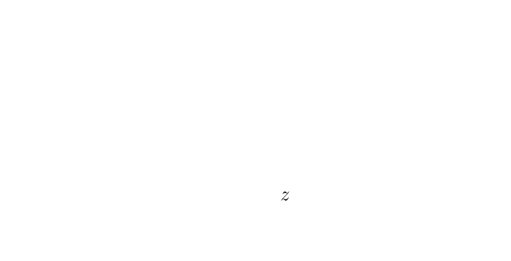
Figure 1: (a) The Kretschmann invariant $\mathcal{K}=R_{\mu\nu\rho\sigma}R^{\mu\nu\rho\sigma}$ evaluated on the spacetime as a solution of EOMs. The classical singularity at $z=x-t=0$ (the coordinate origin) is resolved with non-singular spacetime with finite $\mathcal{K}$. The $z$-axis in the Lemaître-type coordinates is the spatial slice when fixing $t$, while parametrizing the time evolution if $x$ is fixed. Both $z\to\pm\infty$ are low curvature regimes, in which the solution reduces to Schwarzschild spacetime as $z\to\infty$, and reduces to ${\rm dS}_{2}\times S^{2}$ as $z\to-\infty$. In the high curvature regime demonstrated in the plot, the solution contains 2 groups of local maxima of $\mathcal{K}$ on $z\in[-8,4]\equiv N_{0}$ and $z\in[-295,-280]\equiv N_{<}$. The Maxima of $\mathcal{K}$ on this 2 intervals are $5913.2$ and $5075.1$ respectively. (b) Details of local maxima of $\mathcal{K}$ on $z\in[-8,4]$. (c) Details of local maxima of $\mathcal{K}$ on $z\in[-295,-280]$. Values of parameters for this solution are $z_{0}=3\times 10^{8}$, $\Delta=0.1$, $\beta=1$, $R_{s}=10^{8}$.

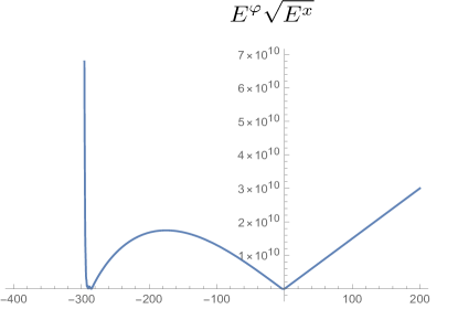
Figure 2: Plot of spatial volume element $E^{\varphi}(z)\sqrt{E^{x}(z)}$ and its bounces. Values of parameters for this solution are $z_{0}=3\times 10^{8}$, $\Delta=0.1$, $\beta=1$, $R_{s}=10^{8}$.

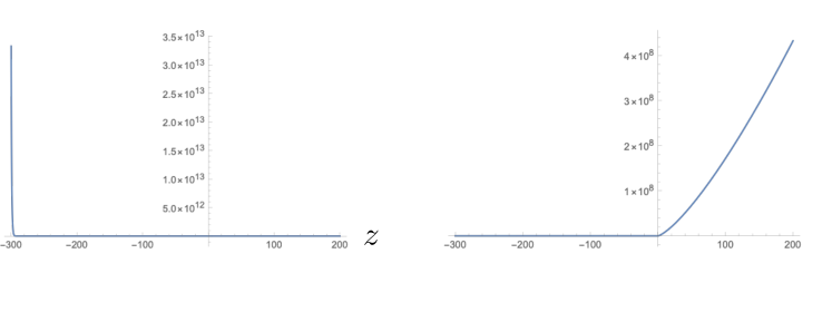
Figure 3: (a) Plot of $E^{\varphi}(z)$. (b) Plot of $E^{x}(z)$. Values of parameters for this solution are $z_{0}=3\times 10^{8}$, $\Delta=0.1$, $\beta=1$, $R_{s}=10^{8}$.

The strategy of finding numerical solutions to Eq.74 is the following: Since both $E^{x}$ and $E^{\varphi}$ are large in the semiclassical regime $z\gg 1$, and the initial condition is at $z_{0}\gg 1$, it is more efficient to change variables:

$$v_{1}(z)=\ln E^{x}(z),\quad v_{2}(z)=\ln E^{\varphi}(z),$$ (92)

and express EOMs in terms of $K_{1},K_{2},v_{1},v_{2}$:

$$\frac{\mathrm{d}}{\mathrm{d}z}\left[\begin{array}[]{c}v_{1}\\ v_{2}\\ K_{1}\\ K_{2}\end{array}\right]=\left[\begin{array}[]{c}F_{1}\left(v_{1},v_{2},K_{1},K_{2}\right)\\ F_{2}\left(v_{1},v_{2},K_{1},K_{2}\right)\\ G_{1}\left(v_{1},v_{2},K_{1},K_{2}\right)\\ G_{2}\left(v_{1},v_{2},K_{1},K_{2}\right)\end{array}\right].$$ (101)

Explicit expressions of (101) are given in github . $v_{1},v_{2}$ are not large in $z\gg 1$, so less numerical errors are produced at the early stage of numerical evolution in $z$. In the $z$-evolution across $z=0$ and toward $-\infty$, $E^{x}$ is suppressed and stabilized at a nonzero constant value, while $E^{\varphi}$ grows exponentially as $-z$ goes large (see Figure 3).

In the region where $E^{\varphi}$ is exponentially large, we can expand EOMs 74 in $1/E^{\varphi}$, and neglect $O(1/E^{\varphi})$ to simplify the EOMs:

$$\frac{1}{4E^{x}{}}+K_{1}{}^{\prime}-\frac{\sin\left(2\beta\sqrt{\Delta}K_{1}{}\right)\sin\left(\beta\sqrt{\Delta}K_{2}{}\right)}{2\beta^{2}\Delta}-\frac{K_{1}{}\sin\left(\beta\sqrt{\Delta}K_{2}{}\right)\cos\left(\beta\sqrt{\Delta}K_{2}{}\right)}{\beta\sqrt{\Delta}}$$

$$-\frac{K_{1}{}\sin\left(2\beta\sqrt{\Delta}K_{1}{}\right)\cos\left(\beta\sqrt{\Delta}K_{2}{}\right)}{\beta\sqrt{\Delta}}+\frac{K_{2}{}\sin\left(2\beta\sqrt{\Delta}K_{1}{}\right)\cos\left(\beta\sqrt{\Delta}K_{2}{}\right)}{2\beta\sqrt{\Delta}}-\frac{\sin^{2}\left(\beta\sqrt{\Delta}K_{2}{}\right)}{4\beta^{2}\Delta}$$

$$+\frac{K_{2}{}\sin\left(\beta\sqrt{\Delta}K_{2}{}\right)\cos\left(\beta\sqrt{\Delta}K_{2}{}\right)}{2\beta\sqrt{\Delta}}=0,$$ (102)

$$-\frac{1}{2E^{x}{}}-\frac{\sin\left(2\beta\sqrt{\Delta}K_{1}{}\right)\sin\left(\beta\sqrt{\Delta}K_{2}{}\right)}{\beta^{2}\Delta}+\frac{2K_{1}{}\cos\left(2\beta\sqrt{\Delta}K_{1}{}\right)\sin\left(\beta\sqrt{\Delta}K_{2}{}\right)}{\beta\sqrt{\Delta}}$$

$$-\frac{K_{2}{}\cos\left(2\beta\sqrt{\Delta}K_{1}{}\right)\sin\left(\beta\sqrt{\Delta}K_{2}{}\right)}{\beta\sqrt{\Delta}}+K_{2}{}^{\prime}-\frac{\sin^{2}\left(\beta\sqrt{\Delta}K_{2}{}\right)}{2\beta^{2}\Delta}=0,$$ (103)

$$E^{x}{}^{\prime}+\frac{2E^{x}{}\cos\left(2\beta\sqrt{\Delta}K_{1}{}\right)\sin\left(\beta\sqrt{\Delta}K_{2}{}\right)}{\beta\sqrt{\Delta}}=0,$$ (104)

$$\frac{\sin\left(2\beta\sqrt{\Delta}K_{1}{}\right)\cos\left(\beta\sqrt{\Delta}K_{2}{}\right)}{\beta\sqrt{\Delta}}+\frac{\sin\left(\beta\sqrt{\Delta}K_{2}{}\right)\cos\left(\beta\sqrt{\Delta}K_{2}{}\right)}{\beta\sqrt{\Delta}}+v_{2}^{\prime}=0,$$ (105)

where $v_{2}=\ln E^{\varphi}$ only appears in the Eq.105.

In practice, the numerical $z$-evolution from $z_{0}$ to $z<0$ follows the EOMs 101 until certain $z_{mid}<0$ where $E^{\varphi}$ is too large. Then the solution $E^{x},E^{\varphi},K_{1},K_{2}$ of 101 evaluated at $z_{mid}$ serves as the initial condition for Eqs.102 - 105, which can be further evolved to arbitrarily large $-z$. The approximation in Eqs.102 - 105 by neglecting $O(1/E^{\varphi})$ is consistent because the solution $E^{\varphi}$ keeps growing exponentially as $z\to-\infty$, while all other quantities are bounded by $O(1)$. A full solution of the EOMs is given by connecting 2 solutions of 101 and 102 - 105 at $z_{mid}$.

Note that the similar approximation with $E^{\tilde{\varphi}}\gg 1$ can be applied to 55 - 58 and leads to

$$\frac{1}{4E^{\tilde{x}}{}}+\partial_{\tilde{z}}\tilde{K}_{1}-\frac{\sin\left(2\beta\sqrt{\Delta}\tilde{K}_{1}\right)\sin\left(\beta\sqrt{\Delta}\tilde{K}_{2}\right)}{2\beta^{2}\Delta}-\frac{\tilde{K}_{1}\sin\left(\beta\sqrt{\Delta}\tilde{K}_{2}\right)\cos\left(\beta\sqrt{\Delta}\tilde{K}_{2}\right)}{\beta\sqrt{\Delta}}$$

$$+\frac{\tilde{K}_{1}\sin\left(2\beta\sqrt{\Delta}\tilde{K}_{1}\right)\cos\left(\beta\sqrt{\Delta}\tilde{K}_{2}\right)}{\beta\sqrt{\Delta}}+\frac{\tilde{K}_{2}\sin\left(2\beta\sqrt{\Delta}\tilde{K}_{1}\right)\cos\left(\beta\sqrt{\Delta}\tilde{K}_{2}\right)}{2\beta\sqrt{\Delta}}+\frac{\sin^{2}\left(\beta\sqrt{\Delta}\tilde{K}_{2}\right)}{4\beta^{2}\Delta}$$

$$-\frac{\tilde{K}_{2}\sin\left(\beta\sqrt{\Delta}\tilde{K}_{2}\right)\cos\left(\beta\sqrt{\Delta}\tilde{K}_{2}\right)}{2\beta\sqrt{\Delta}}=0,$$ (106)

$$\frac{1}{2E^{\tilde{x}}{}}+\frac{\sin\left(2\beta\sqrt{\Delta}\tilde{K}_{1}\right)\sin\left(\beta\sqrt{\Delta}\tilde{K}_{2}\right)}{\beta^{2}\Delta}-\frac{2\tilde{K}_{1}\cos\left(2\beta\sqrt{\Delta}\tilde{K}_{1}\right)\sin\left(\beta\sqrt{\Delta}\tilde{K}_{2}\right)}{\beta\sqrt{\Delta}}$$

$$-\frac{\tilde{K}_{2}\cos\left(2\beta\sqrt{\Delta}\tilde{K}_{1}\right)\sin\left(\beta\sqrt{\Delta}\tilde{K}_{2}\right)}{\beta\sqrt{\Delta}}+\partial_{\tilde{z}}\tilde{K}_{2}-\frac{\sin^{2}\left(\beta\sqrt{\Delta}\tilde{K}_{2}\right)}{2\beta^{2}\Delta}=0,$$ (107)

$$\partial_{\tilde{z}}E^{\tilde{x}}+\frac{2E^{\tilde{x}}{}\cos\left(2\beta\sqrt{\Delta}\tilde{K}_{1}\right)\sin\left(\beta\sqrt{\Delta}\tilde{K}_{2}\right)}{\beta\sqrt{\Delta}}=0,$$ (108)

$$-\frac{\sin\left(2\beta\sqrt{\Delta}\tilde{K}_{1}\right)\cos\left(\beta\sqrt{\Delta}\tilde{K}_{2}\right)}{\beta\sqrt{\Delta}}+\frac{\sin\left(\beta\sqrt{\Delta}\tilde{K}_{2}\right)\cos\left(\beta\sqrt{\Delta}\tilde{K}_{2}\right)}{\beta\sqrt{\Delta}}+\partial_{\tilde{z}}\tilde{v}_{2}=0.$$ (109)

where $\tilde{v}_{2}=\ln E^{\tilde{\varphi}}$. Eqs.106-109 relate to Eqs.102-105 by $\tilde{z}=-z$ and transformations 85 - 88.

5.2 Properties of solutions

The numerical solutions exhibit following properties: The spacetime curvature is finite on the entire range of $z$ (from $z_{0}\gg 1$ to negative $z$ with arbitrarily large $|z|$). The classical singularity at $z=0$ is resolved. The entire spacetime is nonsingular and has large but finite curvature at $z=0$. Figure 1 plots the Kretschmann invariant $\mathcal{K}=R_{\mu\nu\rho\sigma}R^{\mu\nu\rho\sigma}$ of the solution. It demonstrates 2 groups of local maxima of $\mathcal{K}$ located respectively in the neighborhood $N_{0}$ of $z=0$ (Figure 1(b)) and in a neighborhood $N_{<}$ of $z<0$ (Figure 1(c)). The oscillatory $\mathcal{K}$ in these 2 neighborhoods indicates strong quantum fluctuations in these regimes. We denote by $\mathcal{K}_{max,0}$ and $\mathcal{K}_{max,<}$ the maximal $\mathcal{K}$ in $N_{0}$ and $N_{<}$ respectively, and test their dependences with respect to $\Delta$ and horizon radius $R_{s}$ (we fix $\beta=1$). The numerics demonstrate that both $\mathcal{K}_{max,0}$ and $\mathcal{K}_{max,<}$ are proportional to $\Delta^{-2}$ (see Figure 4)

$$\mathcal{K}_{max,0}\big{|}_{\beta=1}\simeq\frac{1}{\Delta^{2}}k_{0}(R_{s},\Delta),\quad\mathcal{K}_{max,<}\big{|}_{\beta=1}\simeq\frac{1}{\Delta^{2}}k_{<}(R_{s},\Delta),$$ (110)

The behavior has qualitative similarity with results in Gambini:2020nsf ; Ashtekar:2018cay . The behavior of Kretschmann scalar $\mathcal{K}\sim\Delta^{-2}$ motivates us to understand $\Delta\sim\ell_{P}^{2}$ such that the singularity resolution and bounce of spatial volume (Fig.2) happen at the Planckian curvature. Both $\mathcal{K}_{max,0}$ and $\mathcal{K}_{max,<}$ are Planckian curvatures. In models of LQC and LQG black holes, $\Delta$ is chosen to be the minimal nonzero eigenvalue of the LQG area operator. Here $\mathcal{K}_{max,0}>\mathcal{K}_{max,<}$, and $k_{0},k_{<}$ have mild dependence on $R_{s}$ and $\Delta$ (see Figs.4 and 5). The $R_{s}$ and $\Delta$ dependences in $k_{0},k_{<}$ are subleading corrections. Asymptotically for large negative $z$, $\mathcal{K}$ approaches to be $z$-independent constant whose dependence on $\Delta$ is still $\sim 1/\Delta^{2}$. We come back to this asymptotic behavior shortly.

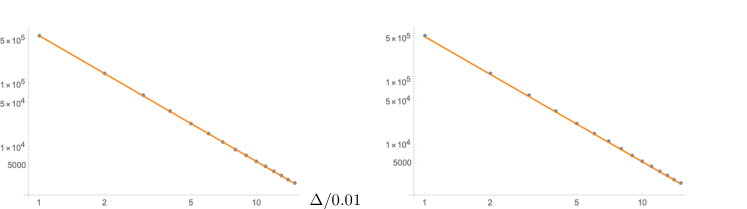
Figure 4: The left panel is the Log-Log plot of $\mathcal{K}_{max,0}$ versus $\Delta$. The right panel is the Log-Log plot of $\mathcal{K}_{max,<}$ versus $\Delta$. The orange straight lines are $constant\times\Delta^{-2}$. Values of parameters are $z_{0}=3\times 10^{8}$, $\Delta=0.01m$ $(m=1,\cdots,15)$, $\beta=1$, $R_{s}=10^{9}$.

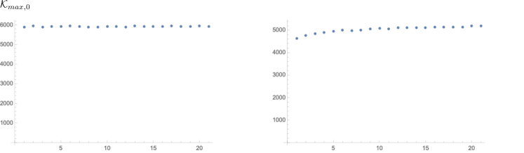
Figure 5: The left panel is the plot of $\mathcal{K}_{max,0}$ versus $R_{s}$. The right panel is the plot of $\mathcal{K}_{max,<}$ versus $R_{s}$. Values of parameters are $z_{0}=3\times 10^{8}$, $\Delta=0.1$, $\beta=1$, $R_{s}=10^{7}m$ $(m=1,\cdots,21)$.

In the regime $z>0$ and far away from $N_{0}$, the solution is semiclassical and reduces to the Schwarzschild spacetime in Lemaître coordinates. The quantum effect is negligible in this regime. It is clear from EOMs 51 - 54 that as far as $K_{x},K_{\varphi}$ do not blow up, the classical Schwarzschild geometry is approximately a solution to 51 - 54 up to corrections of $O(\sqrt{\Delta})$. In particular, the numerical solution indicates that the quantum correction at the event horizon $z=\frac{2}{3}R_{s}$ is negligible. $z=\frac{2}{3}R_{s}$ is a marginal trapped surface with $\Theta_{k}=0$ and $\Theta_{l}<0$ where $\Theta_{k}$ and $\Theta_{l}$ are outward and inward null expansions (see Figure 6).

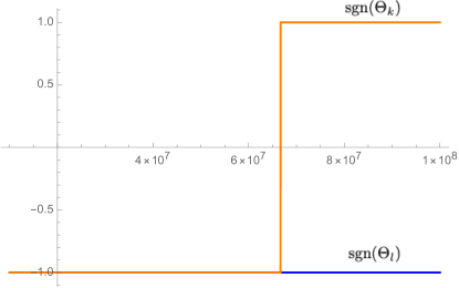
Figure 6: Plots of $\mathrm{sgn}(\Theta_{k})$ (orange) and $\mathrm{sgn}(\Theta_{l})$ (blue). $\Theta_{k}=0$ is at $z_{s}\simeq 6.66666\times 10^{7}\simeq\frac{2}{3}R_{s}$. The relative correction $\frac{|z_{s}-\frac{2}{3}R_{s}|}{\frac{2}{3}R_{s}}\sim 10^{-8}$ (from numerics using Mathematica) is small. Values of parameters for this solution are $z_{0}=3\times 10^{8}$, $\Delta=0.1$, $\beta=1$, $R_{s}=10^{8}$.

The other asymptotic regime is in the opposite side where $z<0$ and $-z$ is large. In this regime $E^{x}$ approaches a constant, denoted by $r_{0}^{2}$, and $E^{\varphi}$ grows exponentially:

$$E^{x}(z)\sim r_{0}^{2},\quad\Lambda(z)=\frac{E^{\varphi}(z)}{\sqrt{E^{x}(z)}}\sim e^{-\alpha_{1}-\alpha^{-1}_{0}z},\quad z\to-\infty,$$ (111)

$r_{0},\alpha_{0},\alpha_{1}$ can be obtained numerically (see Figure 7). $E^{x}(z)$ approaching to constant as $z\to-\infty$ ($x\to-\infty$ when fixing $t$) fulfills the boundary condition 48 discussed earlier.

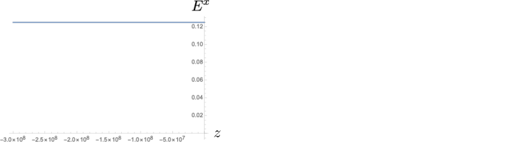
Figure 7: The left panel plots the asymptotic behavior of $E^{x}$ as $-z$ goes large. The right panel plots the asymptotic behavior of $\ln(\Lambda)$ which can be fit by the linear function $-371.252-1.17395z$. Values of parameters are $z_{0}=3\times 10^{8}$, $\Delta=0.1$, $\beta=1$, $R_{s}=10^{8}$.

Recall that the spacetime metric is given by 24, the simple asymptotic behavior 111 indicates that at $z\to-\infty$ is the metric looks like ${\rm dS}_{2}\times S^{2}$: a product of 2-dimensional de Sitter (dS) spacetime and 2-sphere,

$$\mathrm{d}s^{2}\sim-\mathrm{d}t^{2}+e^{-2\alpha_{1}+2\alpha^{-1}_{0}(t-x)}\mathrm{d}x^{2}+r_{0}^{2}\left(\mathrm{d}\theta^{2}+\sin^{2}\theta\mathrm{d}\varphi^{2}\right)$$ (112)

A coordinate transformation $x\to\eta$ with $\mathrm{d}\eta=e^{-\alpha_{1}-\alpha^{-1}_{0}x}\mathrm{d}x$ makes 112 as $\mathrm{d}s^{2}\sim-\mathrm{d}t^{2}+e^{2\alpha^{-1}_{0}t}\mathrm{d}\eta^{2}+r_{0}^{2}\left(\mathrm{d}\theta^{2}+\sin^{2}\theta\mathrm{d}\varphi^{2}\right)$ where $(t,\eta)$ is the inflationary coordinate in the ${\rm dS}_{2}$ . The dS radius is given by $\alpha_{0}$ and the $S^{2}$ sphere radius is constantly $r_{0}$. The numerical result indicates that $\alpha_{0}$ and $r_{0}$ are purely quantum effects:

$$r_{0}\simeq 1.11724\Delta^{1/2},\quad\alpha_{0}\simeq 2.69371\Delta^{1/2},\quad(\text{at}\ \beta=1),$$ (113)

and independent of $R_{s}$ (see Figures 8 and 9). The Kretschmann invariant $\mathcal{K}$ approaches constant

$$\mathcal{K}\sim 4\left(\frac{1}{\alpha_{0}^{4}}+\frac{1}{r_{0}^{4}}\right)\simeq\frac{2.64325}{\Delta^{2}},$$ (114)

as indicated in Figure 1. The asymptotical regime as $z\to-\infty$ still has Planckian curvature. $\alpha_{1}$ depends on both $\Delta$ and $R_{s}$ (see Figure 10). Although the asymptotic ${\rm dS}_{2}\times S^{2}$ geometry is independent of $R_{s}$ or the mass of black hole, the dust coordinate $x$ in the geometry depends on $R_{s}$ since $\alpha_{1}$ depends on $R_{s}$.

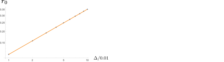
Figure 8: The left panel is the Log-Log plot of $r_{0}$ versus $\Delta$. Blue dots are $r_{0}$ at different values of $\Delta$. The orange line is the fit function $r_{0}=1.117\sqrt{\Delta}$. The right panel is the Log-Log plot of $\alpha_{0}$ versus $\Delta$. Blue dots are $\alpha_{0}$ at different values of $\Delta$. The orange line is the fit function $\alpha_{0}=2.694\sqrt{\Delta}$. Values of parameters are $z_{0}=3\times 10^{8}$, $\Delta=0.01m$ $(m=1,\cdots,10)$, $\beta=1$, $R_{s}=10^{8}$.

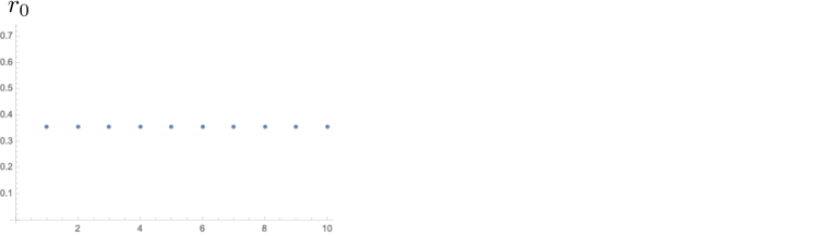
Figure 9: The left panel plots of $r_{0}$ at different values of $R_{s}$. The right panel plots of $\alpha_{0}$ at different values of $R_{s}$. Both $\alpha_{0}$ and $r_{0}$ are constant in $R_{s}$. Values of parameters are $z_{0}=3\times 10^{8}$, $\Delta=0.1$, $\beta=1$, $R_{s}=10^{7}m$ $(m=1,\cdots,10)$.

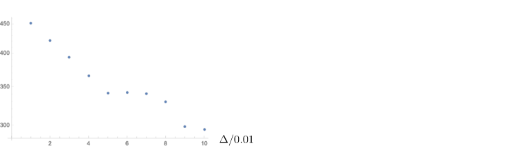
Figure 10: Plots of $\alpha_{1}$ versus different values of $\Delta$ and $R_{s}$. Values of other parameters are $z_{0}=3\times 10^{8}$ and $\beta=1$.

${\rm dS}_{2}\times S^{2}$ with $r_{0}\neq\alpha_{0}$ is also known as the charged Nariai geometry. It can be obtained as the near horizon limit of the (near) extremal Reissner-Nordstrom-de Sitter (RN-dS) spacetime where the cosmological horizon and event horizon coincide Bousso:1996pn ; Hawking:1995ap . The relation between LQG black hole and the Nariai geometry has been proposed in earlier studies of effective dynamics using the Kantowski-Sachs foliation of the black hole interior Bohmer:2007wi ; Boehmer:2008fz . However as is pointed out in Ashtekar:2018cay that the analysis in Bohmer:2007wi ; Boehmer:2008fz suffers from 2 problems: (1) their $\bar{\mu}$-scheme model of black hole interior produce large quantum effect near the event horizon which is of low curvature, and (2) the area of $S^{2}$ is even smaller than the minimal area gap $\Delta$ at certain stage of the time evolution, inconsistent with the $\bar{\mu}$-scheme treatment of holonomies ($S^{2}$ has no room for the $\bar{\mu}$-scheme holonomy since it has to be around an area of $\Delta$). Our analysis does not have these problems: Firstly the quantum effect is negligible in the low curvature regime including the event horizon as discussed above. Secondly, numerical results indicate that the area of $S^{2}$ is always larger than $\Delta$ during the evolution (see Figure 11).

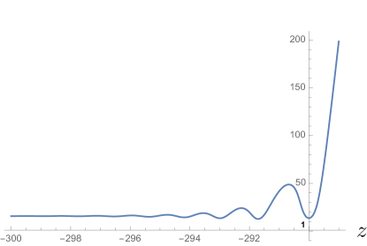
Figure 11: Minima of the $S^{2}$ area $4\pi E^{x}$ divided by $\Delta$. The axis origin is $(-290,1)$. Values of parameters for this solution are $z_{0}=3\times 10^{8}$, $\Delta=0.1$, $\beta=1$, $R_{s}=10^{8}$.

It may be more proper to view the charged Nariai geometry ${\rm dS}_{2}\times S^{2}$ here as a quantum geometry, since both $E^{x}=r_{0}^{2}$ and the dS radius $\alpha_{0}$ is of $O(\sqrt{\Delta})$. ${\rm dS}_{2}\times S^{2}$ corresponds quantum states $|r_{0},\alpha_{0};\alpha_{1}\rangle$ such that when $z\to-\infty$:

$$\langle r_{0},\alpha_{0};\alpha_{1}|\hat{E}^{x}(z)|r_{0},\alpha_{0};\alpha_{1}\rangle=r_{0}^{2},\quad\langle r_{0},\alpha_{0};\alpha_{1}|\hat{E}^{\varphi}(z)|r_{0},\alpha_{0};\alpha_{1}\rangle=r_{0}e^{-\alpha_{1}-\alpha_{0}^{-1}z}.$$ (115)

$r_{0}\sim\sqrt{\Delta}$ is of Planck size, so that quantum fluctuations of ${E}^{x}$ given by $|r_{0},\alpha_{0};\alpha_{1}\rangle$ must be small in order to trust this effective geometry. Therefore the charged Nariai geometry should have large quantum fluctuation of $K_{x}$ by the uncertainty principle.

It is interesting that these states $|r_{0},\alpha_{0};\alpha_{1}\rangle$ depend on the additional parameter $\alpha_{1}$ which indicates that ${\rm dS}_{2}\times S^{2}$ is not a single state, but has infinite degeneracy from the quantum point of view. Although different values of $\alpha_{1}$ correspond to the same spacetime geometry, and are related by diffeomorphisms, here they indeed correspond to different physical states since we start with the reduced phase space formulation where gravity is deparametrized by dust fields. All states $|r_{0},\alpha_{0};\alpha_{1}\rangle$ corresponding to ${\rm dS}_{2}\times S^{2}$ should span a Hilbert space $\mathcal{H}_{\rm dS_{2}\times S^{2}}$. We come back to discussing more details of $\mathcal{H}_{\rm dS_{2}\times S^{2}}$ in Section 10.

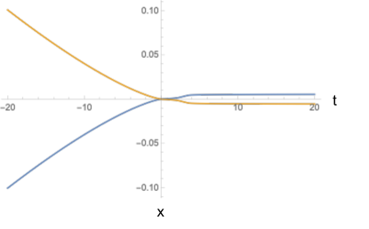
Figure 12: Null rays viewed in the $t$-$x$ dust coordinates. The orange (blue) curve is generated by $U^{\alpha}$ ($V^{\alpha}$).

Figure 13: The quantum effective black hole spacetime covered by $(t,x,\theta,\varphi)$ coordinate. $\mathcal{S}$ (black curve) is a typical spatial slice with constant $t$. Dashed curves are another spatial slice in the far past. The green line illustrate the event horizon, which bounds the black hole region. The grey triangular region has strong quantum fluctuation and has Plankian curvature. It enclose the classical singularity at $z=x-t=0$ near its past boundary. At the future boundary of the patch, the asymptotic geometry is ${\rm dS}_{2}\times S^{2}$ with Planckian radii.

Viewing ${\rm dS}_{2}\times S^{2}$ to be the asymptotic geometry, we draw the Penrose diagram of the effective spacetime in Figure 13. The resulting spacetime has a complete future infinity since ${\rm dS}_{2}\times S^{2}$ is complete. The dust time $t$ can extend to $t\to\infty$ in the spacetime as the inflationary coordinate in ${\rm dS}_{2}$.

We compute the Einstein tensor of the solution and define the quantum effective stress-energy tensor $T^{\rm(eff)}_{\mu\nu}$ by $R_{\mu\nu}-\frac{1}{2}g_{\mu\nu}R=8\pi GT^{\rm(eff)}_{\mu\nu}$. We find $T^{\rm(eff)}_{\mu\nu}$ violate the average null energy condition, i.e. $\int T^{\rm(eff)}_{UU}\mathrm{d}U$ and $\int T^{\rm(eff)}_{VV}\mathrm{d}V$ are negative. In concrete, when parameters are e.g. $z_{0}=3\times 10^{8}$, $\Delta=0.1$, $\beta=1$, $R_{s}=10^{8}$, $\int T^{\rm(eff)}_{UU}\mathrm{d}U\simeq\int T^{\rm(eff)}_{VV}\mathrm{d}V\simeq-2.29749$. the main contributions to $\int T^{\rm(eff)}_{UU}\mathrm{d}U,\int T^{\rm(eff)}_{VV}\mathrm{d}V$ are from the regions with local maxima of $\mathcal{K}$. Here $T^{\rm(eff)}_{\mu\nu}$ does not correspond to any physical matter (the dust density is approximately zero in this solution), but rather is an effective account of the LQG effect in the black hole.

The numerical errors can be tested by inserting numerical solutions back into the EOMs. We find the EOMs are satisfied by solutions up to numerical errors which are bounded by $\sim 10^{-21}$ with Julia and by $\sim 10^{-8}$ with Mathematica github .

5.3 Perturbation and stability

Figure 14: Plots of absolute values $|p_{1}(\xi,k)|,|p_{2}(\xi,k)|,|c_{1}(\xi,k)|,|c_{2}(\xi,k)|$ of a typical solution of perturbations, at $k=1.0076$ and random initial conditions $\sim 10^{-5}$ (at $z_{initial}=10^{3}$). The orange curves are for $p_{1},c_{1}$ while the blue curves are for $p_{2},c_{2}$. Asymptotically as $z\to-\infty$, $p_{1},c_{1},c_{2}$ damp off while $p_{2}$ stabilizes with a finite tail, consistent with the analytic result 122-125.

In this subsection, we exam the stability of the asymptotic geometry ${\rm dS}_{2}\times S^{2}$ by turning on some perturbations. We still assume perturbations to satisfy the spherical symmetry, so we are going to linearize EOMs 51 - 54 at the asymptotic background ${\rm dS}_{2}\times S^{2}$. In practice, we make the change of variable from $(E^{x},E^{\varphi},K_{x},K_{\varphi})$ to $(E^{x},E^{\varphi},K_{1},K_{2})$ where

$$K_{1}=\frac{\sqrt{E^{x}{}}K_{x}{}}{E^{\varphi}{}},\quad K_{2}=\frac{K_{\varphi}{}}{\sqrt{E^{x}{}}}.$$ (116)

and insert in the EOMs the perturbation ansatz:

$$K_{1}(t,x) = \mathring{K}_{1}(z)\left[1+\varepsilon c_{1}(t,x)\right],\quad K_{2}(t,x)=\mathring{K}_{2}(z)\left[1+\varepsilon c_{2}(t,x)\right]$$ (117)

$$E^{x}(t,x) = \mathring{E}^{x}(z)\left[1+\varepsilon p_{1}(t,x)\right],\quad E^{\varphi}(t,x)=\mathring{E}^{\varphi}(z)\left[1+\varepsilon p_{2}(t,x)\right]$$ (118)

where $\varepsilon\ll 1$ and $z=x-t$. On ${\rm dS}_{2}\times S^{2}$, $\mathring{E}^{x}(z)=r_{0}^{2}$, $\mathring{E}^{\varphi}(z)=r_{0}e^{-\alpha_{1}-\alpha_{0}^{-1}z}$, and $\mathring{K}_{1},\mathring{K}_{2},r_{0},\alpha_{0},\alpha_{1}$ are constants. For example, the numerical solution with parameters $\Delta=0.1,\ R_{s}=10^{8},\ \beta=1$ gives

$$\mathring{K}_{1}=2.48365,\quad\mathring{K}_{2}=-1.85699,\quad r_{0}^{2}=0.124823,\quad\alpha_{1}=321.05,\quad\alpha^{-1}_{0}=1.17395.$$ (119)

When inserting the ansatz and expand the EOMs in $\varepsilon$, $O(\varepsilon^{0})$ is identically satisfied for the asymptotic background, and $O(\varepsilon^{1})$ gives

$$0.0528952p_{1}^{(1,0)}(t,x)+0.0450575p_{1}^{(2,0)}(t,x)+0.2p_{1}(t,x)+0.34073p_{2}^{(1,0)}(t,x)=0,$$ (120)

$$-0.170365p_{1}^{(1,0)}(t,x)-0.2p_{1}(t,x)+0.0623492p_{2}^{(1,0)}(t,x)+0.0531106p_{2}^{(2,0)}(t,x)=0$$ (121)

after eliminating $c_{1},c_{2}$ and neglecting terms that are exponentially suppressed as $t\to\infty$, since we are interested in the asymptotic behavior of perturbations as $t\to\infty$ ($z\to-\infty$) where ${\rm dS}_{2}\times S^{2}$ is located. The solution is given by

$${p_{1}}(t,x) = e^{-0.586975t}\big{(}\sin(5.32462t)\left[0.203424f_{1}(x)+0.187807f_{2}(x)-0.0290504f_{4}(x)\right]$$ (122)

$$+\ \cos(5.32462t)\left[0.154682f_{1}(x)+0.263524f_{4}(x)\right]\big{)}$$

$$+\ e^{-1.17395t}\left[0.845318f_{1}(x)-0.263524f_{4}(x)\right],$$

$${p_{2}}(t,x) = -0.291431f_{1}(x)+0.111783f_{2}(x)+f_{3}(x)+0.131762f_{4}(x)$$ (123)

$$+\ e^{-0.586975t}\big{(}\sin(5.32462t)\left[0.0787198f_{1}(x)-0.0123227f_{2}(x)+0.158757f_{4}(x)\right]$$

$$-\ \cos(5.32462t)\left[0.131228f_{1}(x)+0.111783f_{2}(x)\right]\big{)}$$

$$+\ e^{-1.17395t}\left[0.422659f_{1}(x)-0.131762f_{4}(x)\right]$$

$${c_{1}}(t,x) = 0.181674{p_{1}}^{(1,0)}(t,x),\quad{c_{2}}(t,x)=-0.572819{p_{2}}^{(1,0)}(t,x),$$ (124)

where initial perturbations $f_{1},\cdots,f_{4}$ are arbitrary functions of $x$. As $t\to\infty$, asymptotically $p_{1},c_{2},c_{2}$ exponentially damp off while

$$p_{2}\to-0.291431f_{1}(x)+0.111783f_{2}(x)+f_{3}(x)+0.131762f_{4}(x)$$ (125)

is controlled by the initial perturbation. We conclude that the asymptotic geometry ${\rm dS}_{2}\times S^{2}$ is stable with linear perturbations. The perturbation of $p_{2}$ in 125 modifies $\alpha_{1}$ in 111 and effectively defines a transformation in $\mathcal{H}_{\rm dS_{2}\times S^{2}}$ from $|r_{0},\alpha_{0};\alpha_{1}\rangle$ to $|r_{0},\alpha_{0};\alpha_{1}^{\prime}\rangle$. We are going to come back to this point in Section 10. Although ${\rm dS}_{2}\times S^{2}$ is stable with linear perturbations, as we are going to see in Section 8, this ${\rm dS}_{2}\times S^{2}$ geometry may be unstable by non-perturbative quantum effect, and have nontrivial quantum transit by tunneling effect.

We can extend the study of perturbations on the entire effective black hole spacetime. Since the background spacetime metric components only depend on $z$, we can rewrite the perturbations in terms of $\xi=-z=t-x$ and $x$

$$K_{1}(t,x) = \mathring{K}_{1}(z)\left[1+\varepsilon c_{1}(\xi,x)\right],\quad K_{2}(t,x)=\mathring{K}_{2}(z)\left[1+\varepsilon c_{2}(\xi,x)\right]$$ (126)

$$E^{x}(t,x) = \mathring{E}^{x}(z)\left[1+\varepsilon p_{1}(\xi,x)\right],\quad E^{\varphi}(t,x)=\mathring{E}^{\varphi}(z)\left[1+\varepsilon p_{2}(\xi,x)\right]$$ (127)

and make Fourier transformations of perturbations along $x$, e.g.

$$p_{1}(\xi,x)=\int\frac{\mathrm{d}k}{\sqrt{2\pi}}\,p_{1}(\xi,k)e^{-ikx}.$$ (128)

We numerically solve $p_{1}(\xi,k),p_{2}(\xi,k),c_{1}(\xi,k),c_{2}(\xi,k)$ from linearizing EOMs 51 - 54 on the entire effective black hole spacetime studied in the lasted subsection. By choosing randomly $k$ and initial conditions at $\xi\to-\infty$, numerical experiments of generating solutions of perturbations indicate that $p_{1}(\xi,k),p_{2}(\xi,k),c_{1}(\xi,k),c_{2}(\xi,k)$ are always bounded from above in the time evolution, with upper bounds controlled by initial values. A typical example is shown in Figure 14. The asymptotic behaviors of perturbations as $\xi\to\infty$ give $p_{1}(\xi,k),c_{1}(\xi,k),c_{2}(\xi,k)\to 0$ and $p_{2}(\xi,k)$ approaching to constant, consistent with the above analytic result in ${\rm dS}_{2}\times S^{2}$.

6 Picture of black hole evaporation

Figure 15: The picture of quantum effective black hole by taking into account the back-reaction from Hawking radiation. The blue curve is the timelike T-DH of the evaporating black hole. The blue diamond illustrates the regime where the horizon area is comparable to $\Delta$.

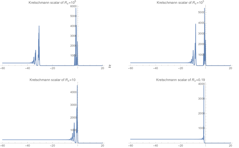
Figure 16: $N_{<}$ and $N_{0}$ become closer as $R_{s}$ decreasing and finally merge. Other parameters for these solutions are $z_{0}=3\times 10^{5}$, $\Delta=0.1$, $\beta=1$. The maximum of $\mathcal{K}$ slowly decreases as $R_{s}$ becoming small.

The quantum correction at the event horizon $z=\frac{2}{3}R_{s}$ is negligible in the black hole solution of effective EOMs. The geometry near and outside the horizon almost has no difference from the classical Schwarzschild spacetime. By turning on quantum field perturbations, the Hawking’s original derivation of black hole evaporation happening near the horizon carries over to the black hole spacetime obtained here. The quantum correction from nonzero $\Delta$ to Hawking’s derivation is negligible. The back-reaction from Hawking radiation reduces the black hole mass and causes the horizon to shrink. Then the event horizon should be replaced by the trapping dynamical horizon (T-DH). A T-DH is a 3-dimensional time-like submanifold foliated by 2-dimensional surfaces $\mathfrak{h}$ with 2-sphere topology, so that at each leaf $\mathfrak{h}$, $\Theta_{k}=0$ and $\Theta_{l}<0$ where $\Theta_{k}$ and $\Theta_{l}$ are expansions of outward and inward null normals of $\mathfrak{h}$ Ashtekar:2003hk . Moreover, for the semiclassical spacetime outside and far from the black hole, the future null infinity $\mathscr{I}^{+}$ is extended until the “last ray”: the last Hawking particle radiated from the black hole before the evaporation stops. The picture of quantum effective black hole spacetime is illustrated in Figure 15. The black hole evaporation results in the existence of the classical asymptotic flat regime which we call the Region (I). All future null rays from points in the Region (I) does not intersect with the black hole horizon, in contrast to the spacetime in Figure 13 where the inward future null ray always cross the horizon.

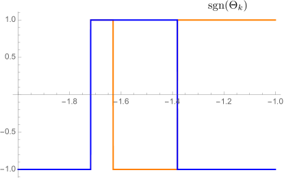
Figure 17: At the instance with $R_{s}=0.19$, the spatial slice $\mathcal{S}_{t}$ has no marginal trapped surface but has transition surfaces with $\Theta_{k}=\Theta_{l}=0$ and a marginal anti-trapped surface (null surface) with $\Theta_{k}=0,\Theta_{l}>0$.

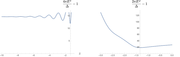
Figure 18: $4\pi E^{x}>\Delta,\ 2\pi E^{\varphi}>\Delta$ is satisfied at $R_{s}=0.19$.

Here we assume the evaporation process is sufficiently slow such that at every instance the spacetime can be approximately described by the solution of effective EOMs with a fixed $R_{s}$. Foliating the spacetime with solutions with different $R_{s}$ approximates the dynamical black hole spacetime.

As an advantage of solutions following the anzatz 64, when we can set a constant $t=t_{0}$, the solution $E^{x}(x-t_{0}),E^{\varphi}(x-t_{0}),K_{x}(x-t_{0}),K_{\varphi}(x-t_{0})$ describe the geometry on a constant $t=t_{0}$ spatial slices $\mathcal{S}$. The 2-sphere $\mathfrak{h}\subset\mathcal{S}$ given by $x-t_{0}=\frac{2}{3}R_{s}$ is a marginal trapped surface with $\Theta_{k}=0$ and $\Theta_{l}<0$ where $\Theta_{k}$ and $\Theta_{l}$ are outward and inward null expansions (see Figure 6). We may implement two different numerical solutions of different parameters $R_{s}(t_{0}),R_{s}(t_{1})$ at different spatial slices $\mathcal{S}_{t_{0}},\mathcal{S}_{t_{1}}$ at two instances $t=t_{0},t_{1}$. The marginal trapped surfaces $\mathfrak{h}(t_{0})$ and $\mathfrak{h}(t_{1})$ are at $x-t_{0}=\frac{2}{3}R_{s}(t_{0})$ and $x-t_{1}=\frac{2}{3}R_{s}(t_{1})$ On $\mathcal{S}_{t_{0}}$ and $\mathcal{S}_{t_{1}}$ respectively. If the evaporation is slow enough, the dynamical black hole can be approximated by a large number of spatial slices $\mathcal{S}_{t}$ carrying different solutions with different horizon radii $R_{s}(t)$ which is monotonically decrease as $t$ growing. The T-DH is foliated by the set of marginal trapped surfaces $\{\mathfrak{h}(t)\}_{t}$, $\mathfrak{h}(t)\subset\mathcal{S}_{t}$.

We run numerical experiments of solving effective EOMs (Eqs.101 by the ansatz 64) with smaller and smaller $R_{s}$ ($R_{s}$ is implemented by the initial condition 89 and 90). From the results, we find that the asymptotic ${\rm dS}_{2}\times S^{2}$ geometry is invariant under changing $R_{s}$, although details of curvature fluctuations and bounces between semiclassical Schwarzschild and ${\rm dS}_{2}\times S^{2}$ can change. In particular two neighborhoods $N_{<}$ and $N_{0}$ (of 2 groups of local maxima of $\mathcal{K}$) become closer as $R_{s}$ decreasing, and finally merge when the horizon area $4\pi R^{2}_{s}$ is comparable to $\Delta$ (see Figure 16). When $N_{<}$ and $N_{0}$ merge, the bounce near $z=0$ looks like a domain wall separating the semiclassical (low curvature) Schwarzschild spacetime and the quantum (high curvature) ${\rm dS}_{2}\times S^{2}$ spacetime.

Remarkably, when $R_{s}$ is small such that $4\pi R^{2}_{s}$ is comparable to $\Delta$, e.g. in the case that $R_{s}=0.19$ in Figure 16, the T-DH disappears and is replaced by a spacelike transition surface with both $\Theta_{k}=0$ and $\Theta_{l}=0$ (see Figure 17). It is followed by a marginal anti-trapped null surface with $\Theta_{k}=0,\Theta_{l}>0$ on the left (at smaller $x$), then followed by anti-trapped and trapped regions (due to small fluctuations of geometry after the bounce, as seen in Figure 16) before approaching to ${\rm dS}_{2}\times S^{2}$. Since the T-DH disappears, Hawking’s derivation of black hole evaporation fails to valid in this regime. We expect the quantum gravity effect to be strong in the region of transition surface since the spacetime curvature at the surface is Planckian. The last ray of Hawking radiation should happen before this instance.

Note that the small $R_{s}$ doesn’t break $4\pi E^{x}>\Delta,\ 2\pi E^{\varphi}>\Delta$ (see Figure 18) as long as $4\pi R_{s}^{2}>\Delta$ , so our results are self-consistent with the starting point of $\bar{\mu}$-scheme regularization.

The region where the Hawking radiation stops is the blue diamond in Figure 15. This region is a neighborhood of the transition surface in Figure 17, and has the strong quantum gravity effect Haggard:2014rza ; Ashtekar:2020ifw since the curvature is Planckian. This region should also be strongly dynamical. Our analysis of the effective dynamics and approximation using foliations of solutions with $R_{s}(t)$ should be not adequate although it provides a preliminary picture of this phase. The rigorous analysis of this region should apply the full theory of LQG. The study on this aspect is beyond the scope of the present paper.

7 Black hole to white hole transition

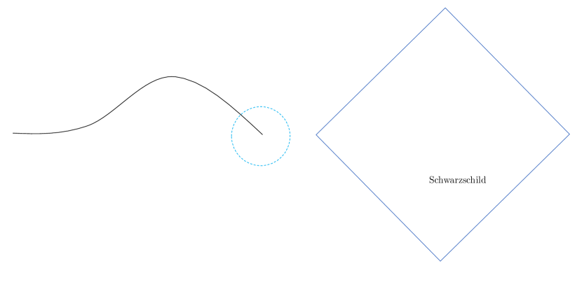
Figure 19: (a) The picture of Region (I) extended from the Schwarzschild spacetime in the past: Assuming the dynamics near $i_{0}$ (enclosed by the light blue dashed circle) can be approximated by classical asymptotically flat geometry with negligible dynamical effect or back-reaction from Hawking radiation. The internal and external geometries of $\mathcal{S}_{\tilde{t}_{0}}$ near $i_{0}$ are consistent with the slice $\mathcal{S}_{{t}_{0}}$ in the close past of the blue diamond; (b) An extended effective spacetime geometry beyond the last ray suggests the black-hole-to-white-hole transition. There is a ${\rm dS}_{2}\times S^{2}$ geometry (denoted by $\widetilde{{\rm dS}_{2}\times S^{2}}$) behind the white hole event horizon (green line). The grey region between ${\rm dS}_{2}\times S^{2}$ and $\widetilde{{\rm dS}_{2}\times S^{2}}$ contains a quantum tunneling. The entire spacetime includs two coordinate patches $({t},{x},{\theta},{\varphi})$ and $(\tilde{t},\tilde{x},\tilde{\theta},\tilde{\varphi})$

.

The black hole spacetime in Figure 15 is incomplete due to the existence of the Region (I). The future null infinity $\mathscr{I}^{+}$ should be extended beyond the last ray of Hawking radiation (see Ashtekar:2010qz for an earlier study of extension in 2d dilaton black hole). We are going to use the effective EOMs of ${\bf H}_{\Delta}$ to derive the extension. We make the following assumptions of Region (I) in order to obtain boundary conditions for the effective EOMs:

1. The quantum dynamics in Region (I) near the spatial infinity $i_{0}$ can be well approximated by the quantum field theory on classical background spacetime. The dynamical effect is weak near $i_{0}$. The spacetime near $i_{0}$ is Schwarzschild with certain ADM mass.

2. For all spatial slices Region (I), their asymptotic geometries (metrics and extrinsic curvatures) near the spatial infinity $i_{0}$ are classical and asymptotically flat. Their geometries are continuous extensions from geometries in the past. Namely there exists a slice $\mathcal{S}_{\tilde{t}_{0}}$ in Region (I) such that its asymptotic geometry near $i_{0}$ should be consistent with the asymptotic geometry of $\mathcal{S}_{t_{0}}$ in the close past of the blue diamond (see Figure 19(a)). In particular, their ADM masses are approximately the same.

We find above assumptions are physically reasonable and should be an excellent approximation of the full quantum dynamics. We note that in the most rigorous treatment where the back-reaction from Hawking radiation to Region (I) are taken into account, the ADM mass of $\mathcal{S}_{\tilde{t}_{0}}$ should in principle include the energy of Hawking radiation, since all Hawking particles register in $\mathcal{S}_{\tilde{t}_{0}}$. However in the present work, we assume the energy density of the Hawking radiation is small and ignore its back-reaction to the geometry.

Now we focus on the asymptotic geometry of Region (I) near the spatial infinity $i_{0}$: The neighborhood of $\mathcal{S}_{\tilde{t}_{0}}$ near infinity has the semiclassical Schwarzschild geometry with $R_{s}=2M_{r}$ obtained from extending the geometry from the past, i.e. from $\mathcal{S}_{t_{0}}$. Here $M_{r}$ is the remnant black hole mass before Hawking radiation stops. We may draw infinitely many spatial slices $\mathcal{S}_{\tilde{t}}$ in Region (I) such that all $\mathcal{S}_{\tilde{t}}$ with $\tilde{t}>\tilde{t}_{0}$ end at $i_{0}$ and live in the future of $\mathcal{S}_{\tilde{t}_{0}}$. For simplicity of the present model, we do not consider to vary the ADM mass in the future of $\mathcal{S}_{\tilde{t}_{0}}$. Neighborhoods of all these slices carry the same semiclassical Schwarzschild spacetime geometry near $i_{0}$. The feature of asymptotic flat geometry is preserved when $\tilde{t}\to\infty$.

The foliation $({t},{x},{\theta},{\varphi})$ cannot be extend to Region (I) due to the strong quantum dynamical effect in the blue diamond region, thus a new foliation by $(\tilde{t},\tilde{x},\tilde{\theta},\tilde{\varphi})$ is necessary for studying the dynamics of the spacetime including $\mathcal{S}_{\tilde{t}_{0}}$ and its future. We impose the following boundary conditions near $i_{0}$ corresponding to $\tilde{z}=\tilde{x}-\tilde{t}\to-\infty$ for slices in Region (I):

$$E^{\tilde{x}}(\tilde{z})\sim-\left(\frac{3}{2}\sqrt{R_{s}}(-\tilde{z})\right)^{4/3},\quad E^{\tilde{\varphi}}(\tilde{z})\sim\sqrt{R_{s}}\left(\frac{3}{2}\sqrt{R_{s}}(-\tilde{z})\right)^{1/3},$$ (129)

$$K_{\tilde{x}}(z)\sim\frac{R_{s}}{3\times 2^{2/3}{3}^{1/3}\left(\sqrt{R_{s}}(-\tilde{z})\right)^{4/3}},\quad K_{\tilde{\varphi}}(\tilde{z})\sim\frac{\left(\frac{2}{3}\right)^{1/3}\sqrt{R_{s}}}{\left({\sqrt{R_{s}}(-\tilde{z})}\right)^{1/3}},$$ (130)

where $R_{s}$ equals $2M_{r}$. We are going to apply the boundary conditions 129 and 130 to the effective EOMs of ${\bf H}_{\Delta}$. The resulting solution extends the effective spacetime beyond the last ray.

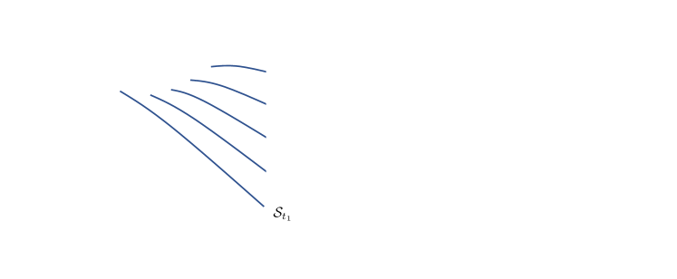
Figure 20: Lemaître foliations $({t},{x},{\theta},{\varphi})$ (left) and $(\tilde{t},\tilde{x},\tilde{\theta},\tilde{\varphi})$ (right) in Kruskal coordinates. Both $t_{1},\cdots,t_{5}$ and $\tilde{t}_{1},\cdots,\tilde{t}_{5}$ are monotonically increasing sequences of time.

The boundary conditions 129 and 130 are obtained as follows: In Region (I) near spatial infinity, the foliation $\mathcal{S}_{\tilde{t}}$ is obtained from $\mathcal{S}_{{t}}$ by the time reflection symmetry $T\to-T$ of the Schwarzschild-Kruskal geometry (see Figure 20 for illustration of spatial slices $\mathcal{S}_{t}$ and $\mathcal{S}_{\tilde{t}}$ when they are in the classical Schwarzschild spacetime). We define diffeomorphism $\mathscr{R}$ maps $\mathcal{S}_{t}$ to $\mathcal{S}_{\tilde{t}}$, and relates the coordinate basis by

$$\mathscr{R}_{*}(\partial/\partial{t})^{\alpha}=-(\partial/\partial\tilde{t})^{\alpha}, \mathscr{R}_{*}(\partial/\partial{x})^{\alpha}=-(\partial/\partial\tilde{x})^{\alpha},$$ (131)

$$\mathscr{R}_{*}(\partial/\partial{\theta})^{\alpha}=(\partial/\partial\tilde{\theta})^{\alpha}, \mathscr{R}_{*}(\partial/\partial{\varphi})^{\alpha}=(\partial/\partial\tilde{\varphi})^{\alpha},$$ (132)

$$\text{equivallently},\quad\tilde{t}({p})=-t(\mathscr{R}^{-1}(p)), \tilde{x}(p)=-x(\mathscr{R}^{-1}(p)),$$ (133)

$$\tilde{\theta}(p)=\theta(\mathscr{R}^{-1}(p)), \tilde{\varphi}(p)=\varphi(\mathscr{R}^{-1}(p)),$$ (134)

for any point $p$ in any $\mathcal{S}_{\tilde{t}}$. Restricting $\mathscr{R}$: $\mathcal{S}_{t}\to\mathcal{S}_{\tilde{t}}$, $E^{\tilde{x}},E^{\tilde{\varphi}}$ in 129 and 130 are obtained by push-forward $\mathscr{R}^{*}E^{\alpha}|_{\mathcal{S}_{\tilde{t}}}=E^{\alpha}|_{\mathcal{S}_{{t}}}$:

$$E^{\tilde{x}}(p) = (\mathscr{R}_{*}E)^{\alpha}(p)(\mathrm{d}\tilde{x})_{\alpha}=E^{\alpha}(\mathscr{R}^{-1}(p))\mathscr{R}^{*}(\mathrm{d}\tilde{x})_{\alpha}=-E^{x}(\mathscr{R}^{-1}(p))$$ (135)

$$E^{\tilde{\varphi}}(p) = (\mathscr{R}_{*}E)^{\alpha}(p)(\mathrm{d}\tilde{\varphi})_{\alpha}=E^{\alpha}(\mathscr{R}^{-1}(p))\mathscr{R}^{*}(\mathrm{d}\tilde{\varphi})_{\alpha}=E^{\varphi}(\mathscr{R}^{-1}(p))$$ (136)

for any point $p\in\mathcal{S}_{\tilde{t}}$. In terms of coordinates, we obtain that as functions, $E^{\tilde{x}}(\tilde{t},\tilde{x})=-E^{{x}}(-\tilde{t},-\tilde{x})$ and $E^{\tilde{\varphi}}(\tilde{t},\tilde{x})=E^{{\varphi}}(-\tilde{t},-\tilde{x})$, which give 129. Since $\mathscr{R}$ leaves the 4d metric invariant, the 4-metric in $(\tilde{t},\tilde{x},\tilde{\theta},\tilde{\varphi})$ is given by

$$\mathrm{d}\tilde{s}^{2}=-\mathrm{d}\tilde{t}^{2}+\Lambda(\tilde{t},\tilde{x})^{2}\mathrm{d}\tilde{x}^{2}+R(\tilde{t},\tilde{x})^{2}\left[\mathrm{d}\tilde{\theta}^{2}+\sin^{2}\tilde{\theta}\mathrm{d}\tilde{\varphi}^{2}\right],\quad\Lambda=\frac{E^{\tilde{\varphi}}}{\sqrt{\left|E^{\tilde{x}}\right|}},\quad R=\sqrt{\left|E^{\tilde{x}}\right|}.$$ (137)

The boundary conditions 130 are given by solving the classical EOMs of ${\bf H}_{0}$ (in the coordinates $(\tilde{t},\tilde{x},\tilde{\theta},\tilde{\varphi})$) with $E^{\tilde{x}}(\tilde{t},\tilde{x}),E^{\tilde{\varphi}}(\tilde{t},\tilde{x})$ given by 129, or equivalently, they can be obtained by computing the extrinsic curvature of $\mathcal{S}_{\tilde{t}}$ .

The extension of black hole exterior geometry in Region (I) can be viewed as the geometry of white hole exterior, as illustrated by Figure 20. This aspect is similar to Haggard:2014rza .

In order to extend the geometry beyond the last ray from Region (I) to the causal future of black hole interior, we apply the effective EOMs of the improved Hamiltonian ${\bf H}_{\Delta}$ and implement the boundary conditions 129 and 130. The effective EOMs are given by Eqs.55 - 58 since we have $E^{x}<0$ by the boundary condition (due to Eq.131).

Recall that the EOMs 55 - 58 in $(\tilde{t},\tilde{x},\tilde{\theta},\tilde{\varphi})$ relate to the EOMs 51 - 54 in $(t,x,\theta,\varphi)$ by identifying $\tilde{x}=-x$, $\tilde{t}=-t$ (thus $z\to\tilde{z}=-z$) and 60 - 63) which consistently match the relation between the boundary conditions 129 and 130 of $E^{\tilde{x}},E^{\tilde{\varphi}},{K}_{\tilde{x}},{K}_{\tilde{\varphi}}$ at $\tilde{z}\to-\infty$ and 89 and 90 of $E^{{x}},E^{{\varphi}},{K}_{x},{K}_{\varphi}$ at $z\to\infty$. We again apply the ansatz $E^{\tilde{x}}(\tilde{t},\tilde{x})=E^{\tilde{x}}(\tilde{z}),\ E^{\tilde{\varphi}}(\tilde{t},\tilde{x})=E^{\tilde{\varphi}}(\tilde{z}),\ K_{\tilde{x}}(\tilde{t},\tilde{x})=K_{\tilde{x}}(\tilde{z}),\ K_{\tilde{\varphi}}(\tilde{t},\tilde{x})=K_{\tilde{\varphi}}(\tilde{z})$ to reduce the PDEs to ODEs (Eqs.83), so that the solution is uniquely determined by the boundary conditions 129 and 130. As a result, the solution $E^{\tilde{x}},E^{\tilde{\varphi}},K_{\tilde{x}},K_{\tilde{\varphi}}$ in $(\tilde{t},\tilde{x},\tilde{\theta},\tilde{\varphi})$ is the spacetime inversion of the solution $E^{{x}},E^{{\varphi}},K_{{x}},K_{{\varphi}}$ in $({t},{x},{\theta},{\varphi})$ by the mapping 60 - 63. All properties of solutions discussed in Section 5.2 is carried over to solutions in $(\tilde{t},\tilde{x},\tilde{\theta},\tilde{\varphi})$ by 60 - 63. In particular, the solution gives asymptotically ${\rm dS}_{2}\times S^{2}$ geometry as $\tilde{z}\to\infty$ ($\tilde{t}\to-\infty$ with fixed $\tilde{x}$ or $\tilde{x}\to\infty$ with fixed $\tilde{t}$)

$$E^{\tilde{x}}(\tilde{z})\sim-r_{0}^{2},\quad E^{\tilde{\varphi}}(\tilde{z})\sim r_{0}e^{-\alpha_{1}+\alpha_{0}^{-1}\tilde{z}},$$ (138)

$$\mathrm{d}\tilde{s}^{2}\sim-\mathrm{d}\tilde{t}^{2}+e^{-2\alpha_{1}+2\alpha^{-1}_{0}(\tilde{x}-\tilde{t})}\mathrm{d}\tilde{x}^{2}+r_{0}^{2}\left(\mathrm{d}\tilde{\theta}^{2}+\sin^{2}\tilde{\theta}\mathrm{d}\tilde{\varphi}^{2}\right),$$ (139)

and constant $\tilde{K}_{1},\tilde{K}_{2}$ ($\tilde{K}_{1}=\frac{\sqrt{-E^{\tilde{x}}}K_{\tilde{x}}}{E^{\tilde{\varphi}}},\ \tilde{K}_{2}=\frac{K_{\tilde{\varphi}}}{\sqrt{-E^{\tilde{x}}}}$), i.e.

$$\tilde{K}_{1}(\tilde{z}\to\infty)={K}_{1}({z}\to-\infty),$$ (140)

$$\tilde{K}_{2}(\tilde{z}\to\infty)=-{K}_{2}({z}\to-\infty),$$ (141)

are constant. The extended spacetime is illustrated by Figure 19(b). $\alpha_{0},r_{0}$ are independent of $R_{s}$ and the same as in 113, while $\alpha_{1}$ depends on $R_{s}$. When we compare to the ${\rm dS}_{2}\times S^{2}$ geometry obtained in Section 5.2 and attempt to glue this 2 version of ${\rm dS}_{2}\times S^{2}$, we find that, if we identify their spatial slices, they have the same $E^{j}_{a}$ (minus sign in $E^{\tilde{x}}$ is due to $\tilde{x}=-x$) when they are obtained from the same $R_{s}$, but they have opposite $K_{j}^{a}$ (no minus sign in $K_{1}$ is again due to $\tilde{x}=-x$), so classically they cannot be glued. By this reason, we denote this new ${\rm dS}_{2}\times S^{2}$ geometry by $\widetilde{{\rm dS}_{2}\times S^{2}}$. The time orientation of $\widetilde{{\rm dS}_{2}\times S^{2}}$ is opposite to ${\rm dS}_{2}\times S^{2}$. The discussion in Section 8 suggests that the transition from ${{\rm dS}_{2}\times S^{2}}$ to $\widetilde{{\rm dS}_{2}\times S^{2}}$ may be due to the quantum tunneling.

The solution $E^{\tilde{x}},E^{\tilde{\varphi}},K_{\tilde{x}},K_{\tilde{\varphi}}$ extends the spacetime geometry beyond the last ray. When fixing $\tilde{t}=\tilde{t}_{0}$, the solution $E^{\tilde{x}}(\tilde{x}-\tilde{t}_{0}),E^{\tilde{\varphi}}(\tilde{x}-\tilde{t}_{0}),K_{\tilde{x}}(\tilde{x}-\tilde{t}_{0}),K_{\tilde{\varphi}}(\tilde{x}-\tilde{t}_{0})$ extends the internal and external geometries of $\mathcal{S}_{\tilde{t}_{0}}$ from Region (I) to the future of the blue diamond. Given the numerical solution, we find at $\tilde{z}=\tilde{x}-\tilde{t}_{0}=-\frac{2}{3}R_{s}$ the marginal anti-trapped surface where $\Theta_{l}=0$ and $\Theta_{k}>0$, while $\tilde{z}>-\frac{2}{3}R_{s}$ is the anti-trapped region with both $\Theta_{k},\Theta_{l}>0$ (see Figure 21). $\Theta_{l}$ and $\Theta_{k}$ are inward and outward null expansion. If $R_{s}=2M_{r}$ is fixed and we do not consider the loss of white hole mass, $\tilde{z}=-\frac{2}{3}R_{s}$ is a null surface being the white hole event horizon. The white hole event horizon may become an spacelike anti-trapping dynamical horizon if the dynamics further reduces $M_{r}$.

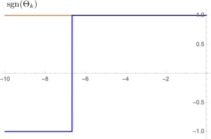
Figure 21: The white hole horizon ($\Theta_{l}=0$ and $\Theta_{k}>0$) at $\tilde{z}=\tilde{z}_{s}=-6.66614$ based on the numerical solution with $R_{s}=10,\ \Delta=0.1$. The relative correction $|\frac{\tilde{z}_{s}-(-\frac{2}{3}R_{s})}{-\frac{2}{3}R_{s}}|\simeq 7\times 10^{-5}$.

8 Evidence of quantum tunneling

The discussion in the last section leaves a question about how ${\rm dS}_{2}\times S^{2}$ and $\widetilde{{\rm dS}_{2}\times S^{2}}$ can be glued to make the black hole interior transit to the white hole interior. To understand this transition, we compute the improved Hamiltonian density at ${\rm dS}_{2}\times S^{2}$

$$\rho=-\frac{\mathcal{C}_{\Delta}}{E^{\varphi}\sqrt{E^{x}}}=\frac{1}{2E^{x}}+\frac{\sin\left(2\beta\sqrt{\Delta}K_{1}\right)\sin\left(\beta\sqrt{\Delta}K_{2}\right)}{\beta^{2}\Delta}+\frac{\sin^{2}\left(\beta\sqrt{\Delta}K_{2}\right)}{2\beta^{2}\Delta},$$ (142)

where we have implemented that $\partial_{x}E^{x}=\partial^{2}_{x}E^{x}=0$. We notice that ${\bf H}_{\Delta}$ has a symmetry of reflection $K_{x}\to-K_{x}$ and $K_{\varphi}\to-K_{\varphi}$ which precisely is the relation between ${\rm dS}_{2}\times S^{2}$ and $\widetilde{{\rm dS}_{2}\times S^{2}}$. $\rho$ is also the density of Gaussian dust by Eqs.10 and 11.

When fixing $E^{x}=r_{0}^{2}$, $\rho$ as a function of $K_{1},K_{2}$ is plotted in Figure 22, where we find that $\rho$ is a double-well effective potential. The values of constant $K_{1},K_{2}$ for ${\rm dS}_{2}\times S^{2}$ and $\widetilde{{\rm dS}_{2}\times S^{2}}$ are located at two zeros of $\rho$ respectively. They are two points in the space of $K_{1},K_{2}$ located respectively in two potential wells. Both ${\rm dS}_{2}\times S^{2}$ and $\widetilde{{\rm dS}_{2}\times S^{2}}$ are not the ground state of $\rho$ since they are not exactly at the minima of $\rho$, although they are close to the minima. The minima of $\rho$ corresponds to $\alpha_{0}\to\infty$ (by computing $\partial_{K_{1}}\rho=\partial_{K_{2}}\rho=0$ and applying Eq.54), which is not possible to approach by the effective dynamics.

Figure 22: The left: Plots of the Hamiltonian density $\rho$ as a function of $K_{1},K_{2}$ in the region $2\beta\sqrt{\Delta}K_{1}\in[-\pi,\pi]$, $\beta\sqrt{\Delta}K_{2}\in[-\pi,\pi]$. The right: the cross section of the left along $K_{1}=2.4836K,K_{2}=-1.8570K$. ${\rm dS}_{2}\times S^{2}$ is located at $K=1$ while $\widetilde{{\rm dS}_{2}\times S^{2}}$ is at $K=-1$.

Figure 22 suggests an analog with the double-well potential in quantum mechanics, which is the standard example of demonstrating quantum tunneling from one potential well to the other. The low energy states of the double-well model are linear combinations of wave packets located respectively in 2 wells.

Both ${\rm dS}_{2}\times S^{2}$ and $\widetilde{{\rm dS}_{2}\times S^{2}}$ should be understood as quantum states (or wave packets) since $r_{0},\alpha_{0}\sim\sqrt{\Delta}$, they should have nonzero quantum fluctuation in $K_{x},K_{\varphi}$. In particular their $K_{x}$ fluctuation should be large since the fluctuation of $E^{x}$ should be small. The analogy with the double-well potential suggests that there should be a quantum tunneling effect transiting from ${\rm dS}_{2}\times S^{2}$ to $\widetilde{{\rm dS}_{2}\times S^{2}}$. We conjecture that the quantum state at the gray region in Figure 19(b) should be a sum over ${\rm dS}_{2}\times S^{2}$ and $\widetilde{{\rm dS}_{2}\times S^{2}}$, namely the state $|r_{0},\alpha_{0};\alpha_{1}\rangle$ in Eq.115 should be

$$|r_{0},\alpha_{0};\alpha_{1}\rangle=\frac{1}{\sqrt{2}}\left(|r_{0},\alpha_{0};\alpha_{1}\rangle_{{\rm dS}_{2}\times S^{2}}+|r_{0},\alpha_{0};\alpha_{1}\rangle_{\widetilde{{\rm dS}_{2}\times,S^{2}}}\right).$$ (143)

which is well-posed since both ${\rm dS}_{2}\times S^{2}$ and $\widetilde{{\rm dS}_{2}\times S^{2}}$ share the same values of $\alpha_{0},\alpha_{1},r_{0}$. It is $|r_{0},\alpha_{0};\alpha_{1}\rangle$ that exists as the final state of the black hole and the initial state of the white hole.

This quantum tunneling may also be described by analytic continuing ${\rm dS}_{2}\times S^{2}$ to Euclidean signature (see e.g. Bousso:1999ms ; Bousso:1996wz for early works on quantum tunneling in the Nariai limit). We write the ${\rm dS}_{2}\times S^{2}$ metric in the global coordinate $\mathrm{d}s^{2}=-\mathrm{d}t^{2}+\alpha_{0}^{2}\cosh^{2}(t/\alpha_{0})\mathrm{d}\psi^{2}+r_{0}^{2}[\mathrm{d}\theta^{2}+\sin^{2}(\theta)\mathrm{d}\varphi^{2}]$ where $\psi$ relates to $x$ by $\mathrm{d}\psi=\alpha_{0}^{-1}e^{-\alpha_{1}-\alpha_{0}^{-1}x}\mathrm{d}x$ (as $t\to\infty$). The analytic continuation $t\to i\tau$ gives

$$\mathrm{d}s^{2}\to\mathrm{d}s^{2}_{E}=\mathrm{d}\tau^{2}+\alpha_{0}^{2}\cos^{2}(\tau/\alpha_{0})\mathrm{d}\psi^{2}+r_{0}^{2}\left[\mathrm{d}\theta^{2}+\sin^{2}(\theta)\mathrm{d}\varphi^{2}\right],$$ (144)

The geometry of the Euclidean metric is $S^{2}\times S^{2}$ whose radii are $\alpha_{0}$ and $r_{0}$. The coordinate transformation $\cos(\tau/\alpha_{0})=\sin(\chi)$ with $\tau/\alpha_{0}\in[-\frac{\pi}{2},\frac{\pi}{2}]$ makes $\mathrm{d}s^{2}_{E}=\alpha_{0}^{2}\left[\mathrm{d}\chi^{2}+\sin^{2}(\chi)\mathrm{d}\psi^{2}\right]+r_{0}^{2}\left[\mathrm{d}\theta^{2}+\sin^{2}(\theta)\mathrm{d}\varphi^{2}\right]$. In the black hole interior, ${\rm dS}_{2}\times S^{2}$ and $\widetilde{{\rm dS}_{2}\times S^{2}}$ cannot be glued classically because the future boundary $t\to\infty$ slice of the former and the past boundary $\tilde{t}\to-\infty$ slice of the latter cannot be glued smoothly. However when we analytic continue to the Euclidean signature and denote their analytic continuation to be $S^{2}\times S^{2}$ and $\widetilde{S^{2}\times S^{2}}$, transiting from $S^{2}\times S^{2}$ to $\widetilde{S^{2}\times S^{2}}$ is a coordinate transformation $\tilde{\tau}/\alpha_{0}=-{\tau}/\alpha_{0}$, $\tilde{\psi}=-\psi$ in the first $S^{2}$. The “future boundary” of $S^{2}\times S^{2}$ at $\tau/\alpha_{0}=\pi/2$ and “past boundary” of $\widetilde{S^{2}\times S^{2}}$ at $\tilde{\tau}/\alpha_{0}=-\pi/2$ are glued at the the south pole where the geometry is smooth (see Figure 23).

The above argument is based on the effective theory. At present we still do not have a derivation of this quantum tunneling from the quantum theory. An analysis of the quantization of ${\bf H}_{\Delta}$ is currently undergoing which is expected to provide more details of the quantum tunneling.

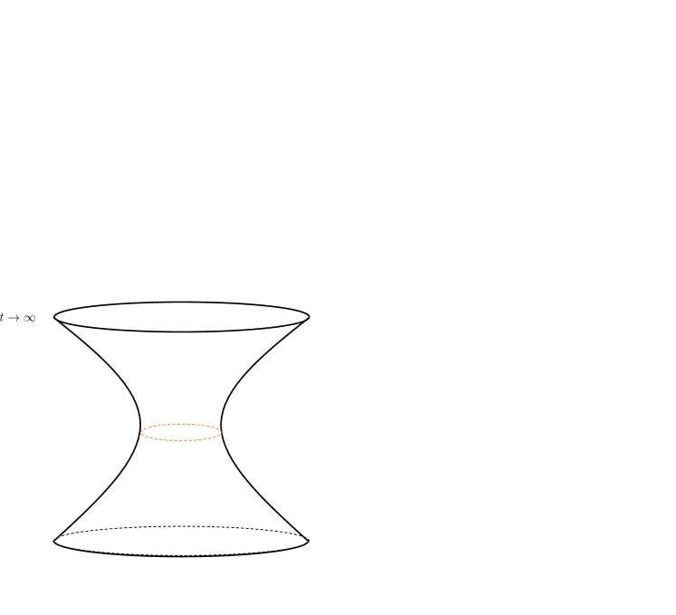
Figure 23: (a) Gluing $t\to\infty$ of ${\rm dS}_{2}\times S^{2}$ to $\tilde{t}\to-\infty$ of $\widetilde{{\rm dS}_{2}\times S^{2}}$ is understood as the quantum tunneling (the $S^{2}$ factor is suppressed in this figure); (b) Both ${\rm dS}_{2}\times S^{2}$ and $\widetilde{{\rm dS}_{2}\times S^{2}}$ are analytic continued to the Euclidean $S^{2}\times S^{2}$. The $S^{2}\times S^{2}$ from ${\rm dS}_{2}\times S^{2}$ has $\tau/\alpha_{0}\in[-\pi/2,\pi/2]$ and $\psi\in[0,2\pi)$ (black half-circle is the $\tau$-obit), while the $\widetilde{S^{2}\times S^{2}}$ from $\widetilde{{\rm dS}_{2}\times S^{2}}$ has $\tilde{\tau}/\alpha_{0}\in[-\pi/2,\pi/2]$ (blue dashed half-circle is the $\tilde{\tau}$-obit). The transition from $S^{2}\times S^{2}$ to $\widetilde{S^{2}\times S^{2}}$ is at the south pole where the geometry is smooth.

9 Chaos

We study linear perturbations in $\widetilde{{\rm dS}_{2}\times S^{2}}$:

$$\tilde{K}_{1}(\tilde{t},\tilde{x}) = \tilde{K}_{1}(\tilde{z}\to\infty)\left[1+\varepsilon\tilde{c}_{1}(\tilde{t},\tilde{x})\right],\quad\tilde{K}_{2}(\tilde{t},\tilde{x})=\tilde{K}_{2}(\tilde{z}\to\infty)\left[1+\varepsilon\tilde{c}_{2}(\tilde{t},\tilde{x})\right]$$ (145)

$$E^{\tilde{x}}(\tilde{t},\tilde{x}) = -r_{0}^{2}\left[1+\varepsilon\tilde{p}_{1}(\tilde{t},\tilde{x})\right],\quad E^{\tilde{\varphi}}(\tilde{t},\tilde{x})=r_{0}e^{-\alpha_{1}+\alpha_{0}^{-1}(\tilde{x}-\tilde{t})}\left[1+\varepsilon\tilde{p}_{2}(\tilde{t},\tilde{x})\right]$$ (146)

where $\varepsilon\ll 1$. These perturbations satisfy the EOMs 55 - 58, and can be obtained from perturbations in the earlier patch $({t},{x},{\theta},{\varphi})$ by the transformation 60 - 63:

$$\tilde{c}_{1}(\tilde{t},\tilde{x}) = \tilde{c}_{1}(-{t},-{x})={c}_{1}({t},{x}),$$ (147)

$$\tilde{c}_{2}(\tilde{t},\tilde{x}) = \tilde{c}_{2}(-{t},-{x})={c}_{2}({t},{x}),$$ (148)

$$\tilde{p}_{1}(\tilde{t},\tilde{x}) = \tilde{p}_{1}(-{t},-{x})={p}_{1}({t},{x}),$$ (149)

$$\tilde{p}_{2}(\tilde{t},\tilde{x}) = \tilde{p}_{2}(-{t},-{x})={p}_{2}({t},{x}).$$ (150)

If we apply to the numerical solution with parameters $\Delta=0.1,\ R_{s}=10^{8},\ \beta=1$, from Eqs.122 - 124, we obtain

$$\tilde{p}_{1}(\tilde{t},\tilde{x}) = e^{0.586975\tilde{t}}\big{(}\sin(-5.32462\tilde{t})\left[0.203424\tilde{f}_{1}(\tilde{x})+0.187807\tilde{f}_{2}(\tilde{x})-0.0290504\tilde{f}_{4}(\tilde{x})\right]$$ (151)

$$+\ \cos(5.32462\tilde{t})\left[0.154682\tilde{f}_{1}(\tilde{x})+0.263524\tilde{f}_{4}(\tilde{x})\right]\big{)}$$

$$+\ e^{1.17395\tilde{t}}\left[0.845318\tilde{f}_{1}(\tilde{x})-0.263524\tilde{f}_{4}(\tilde{x})\right],$$

$$\tilde{p}_{2}(\tilde{t},\tilde{x}) = -0.291431\tilde{f}_{1}(\tilde{x})+0.111783\tilde{f}_{2}(\tilde{x})+\tilde{f}_{3}(\tilde{x})+0.131762\tilde{f}_{4}(\tilde{x})$$ (152)

$$+\ e^{0.586975\tilde{t}}\big{(}\sin(-5.32462\tilde{t})\left[0.0787198\tilde{f}_{1}(\tilde{x})-0.0123227\tilde{f}_{2}(\tilde{x})+0.158757\tilde{f}_{4}(\tilde{x})\right]$$

$$-\ \cos(5.32462\tilde{t})\left[0.131228\tilde{f}_{1}(\tilde{x})+0.111783\tilde{f}_{2}(\tilde{x})\right]\big{)}$$

$$+\ e^{1.17395\tilde{t}}\left[0.422659\tilde{f}_{1}(\tilde{x})-0.131762\tilde{f}_{4}(\tilde{x})\right],$$

$$\tilde{c}_{1}(\tilde{t},\tilde{x}) = -0.181674\partial_{\tilde{t}}\tilde{p}_{1}(\tilde{t},\tilde{x}),\quad\tilde{c}_{2}(\tilde{t},\tilde{x})=0.572819\partial_{\tilde{t}}\tilde{p}_{2}(\tilde{t},\tilde{x}),$$ (153)

where $\tilde{f}_{1},\cdots,\tilde{f}_{4}$ are arbitrary functions of $\tilde{x}$. If initial perturbations are placed at any finite $\tilde{t}=\tilde{t}_{0}$, the time evolution of perturbations is chaotic, i.e. perturbations grow exponentially

$$\Big{(}\tilde{c}_{1}(\tilde{t}),\tilde{c}_{2}(\tilde{t}),\tilde{p}_{1}(\tilde{t}),\tilde{p}_{2}(\tilde{t})\Big{)}\sim e^{\lambda(\tilde{t}-\tilde{t}_{0})}\Big{(}\tilde{c}_{1}(\tilde{t}_{0}),\tilde{c}_{2}(\tilde{t}_{0}),\tilde{p}_{1}(\tilde{t}_{0}),\tilde{p}_{2}(\tilde{t}_{0})\Big{)},$$ (154)

where $\lambda$ is the Lyapunov exponent and relates to the dS₂ radius $\alpha_{0}$

$$\lambda\simeq\alpha_{0}^{-1}.$$ (155)

Numerically $\lambda\simeq 1.173954$ in this example with paramters $\Delta=0.1,\ R_{s}=10^{8},\ \beta=1$. The above relation between $\lambda$ and $\alpha_{0}$ is confirmed by various numerical tests with random choices of parameters.

Because the computation that leads to the chaotic dynamics 154 is based on the effective dynamics which takes into account the quantum gravity effect, this result should indicate the quantum chaos on $\widetilde{{\rm dS}_{2}\times S^{2}}$. It should reflect that for certain expectation value of the squared commutator, e.g.

$$C(\tilde{t}) := -\left\langle\left[\hat{E}^{\tilde{x}}(\tilde{t}),\hat{K}_{\tilde{x}}(\tilde{t}_{0})\right]^{2}\right\rangle$$ (156)

$$\sim \hbar^{2}\left\{{E}^{\tilde{x}}(\tilde{t}),{K}_{\tilde{x}}(\tilde{t}_{0})\right\}^{2}=G^{2}\hbar^{2}\left(\frac{\delta{E}^{\tilde{x}}(\tilde{t})}{\delta{E}^{\tilde{x}}(\tilde{t}_{0})}\right)^{2}\sim G^{2}\hbar^{2}e^{2\lambda(\tilde{t}-\tilde{t}_{0})}.$$ (157)

The quantity $C(\tilde{t})$ is often called the out-of-time-order correlator, and considered as diagnosis of chaos in quantum systems Maldacena:2015waa ; Roberts:2014ifa ; Hosur:2015ylk . Expectation values of commutators should relate to Poisson brackets in the effective dynamics Dapor:2017rwv ; Alesci:2019pbs , while the corresponding Poisson bracket gives the dependence of the final perturbation $\delta{E}^{\tilde{x}}(\tilde{t})$ on small changes in the initial perturbation $\delta{E}^{\tilde{x}}(\tilde{t}_{0})$. The exponential grows in Eq.157 is the expected behavior of $C(\tilde{t})$ in a quantum chaotic system in early time (before the Ehrenfest time $\tilde{t}_{s}-\tilde{t}_{0}\sim\frac{1}{\lambda}\ln\frac{1}{G\hbar}$).

The dS temperature (the Hawking temperature at the cosmological horizon) relates to $\alpha_{0}$ by $T_{\rm dS}=\frac{1}{2\pi\alpha_{0}}$ Figari:1975km . We relate the Lyapunov exponent to the dS temperature by

$$\lambda\simeq 2\pi T_{\rm dS}.$$ (158)

This relation resembles the AdS/CFT black hole butterfly effect where the Lyapunov exponent $\lambda_{\rm CFT}$ of the boundary CFT relates to the black hole Hawking temperature by $\lambda_{\rm CFT}\simeq 2\pi T_{\rm bh}$ Shenker:2013pqa ; Maldacena:2015waa .

The exponential growth lasts only in a small period near $\widetilde{{\rm dS}_{2}\times S^{2}}$. The time evolution in $(\tilde{t},\tilde{x},\tilde{\theta},\tilde{\varphi})$ is just the spacetime inversion of the evolution in $(t,x,\theta,\varphi)$ by 147 - 150. The evolution of perturbations is the same as in Figure 14 but evolving in reverse direction.

10 Infinitely many infrared states in ${\rm dS}_{2}\times S^{2}$

Recall that the asymptotic ${\rm dS}_{2}\times S^{2}$ should be understood as a Hilbert space $\mathcal{H}_{{\rm dS}_{2}\times S^{2}}$ spanned by states $|r_{0},\alpha_{0};\alpha_{1}\rangle$. By Eqs.122 - 125, turning on perturbations changes the value of $\alpha_{1}$ although it leaves ${\rm dS}_{2}\times S^{2}$ geometry invariant. The perturbation defines an operator $\hat{O}_{\varepsilon}$ on $\mathcal{H}_{{\rm dS}_{2}\times S^{2}}$ by

$$\hat{O}_{\varepsilon}|r_{0},\alpha_{0};\alpha_{1}\rangle=|r_{0},\alpha_{0};\alpha_{1}+\varepsilon\delta\alpha_{1}(x)\rangle,\quad\delta\alpha_{1}(x)=-\varepsilon\lim_{t\to\infty}p_{2}(t,x)$$ (159)

The perturbation indicates that the state label $\alpha_{1}$ is generally a function $\alpha_{1}(x)$, although the background geometry has a constant $\alpha_{1}$.

The numerics shows that the background geometry has approximately vanishing dust density $\rho$ throughout the evolution, given that the initial condition 89 and 90 corresponds to the vacuum Schwarzschild spacetime (there exists small numerical error, and $\rho$ is bounded by $\sim 10^{-6}$ throughout the evolution). But perturbations can make the dust density nonvanishing in principle.

Even though perturbations can turn on the dust density, $\rho$ vanishes asymptotically in ${\rm dS}_{2}\times S^{2}$ no matter if perturbations are turned on or not. Indeed let’s consider the PDEs 51 - 54 and the solution with constant $K_{1},K_{2},E^{x}\equiv r_{0}^{2}$ (these cannot be changed by perturbations). $\partial_{t}E^{x}{}=0$ and Eq.53 leads to

$$(a)\quad\cos\left(2\beta\sqrt{\Delta}K_{1}{}\right)=0\quad\text{or}\quad(b)\quad\sin\left(\beta\sqrt{\Delta}K_{2}{}\right)=0$$ (160)

The option ($b$) is dropped since it reduces Eq.52 to $1/E^{x}=0$. The option $(a)$ and Eq.52 gives

$$-\frac{1}{2E^{x}{}}-\frac{\sin\left(2\beta\sqrt{\Delta}K_{1}{}\right)\sin\left(\beta\sqrt{\Delta}K_{2}{}\right)}{\beta^{2}\Delta}-\frac{\sin^{2}\left(\beta\sqrt{\Delta}K_{2}{}\right)}{2\beta^{2}\Delta}=0.$$ (161)

$\rho=\mathcal{C}_{\Delta}/(|E^{\varphi}|\sqrt{|E^{x}|})$ (see Eqs.10 and 11 in the dust coordinate) in ${\rm dS}_{2}\times S^{2}$ reduces to the above left-hand side by ignoring $\partial_{x}E^{x}{}$. On the other hand, in ${\rm dS}_{2}\times S^{2}$, we have $W_{j}=0$ since $W_{j}={P_{j}}/{\sqrt{\det(q)}}=\mathcal{C}_{j}/{\sqrt{\det(q)}}=(\mathcal{C}_{x},0,0)/(|E^{\varphi}|\sqrt{|E^{x}|})$, and by constant $K_{2},E^{x}$,

$$\frac{\mathcal{C}_{x}}{|E^{\varphi}|\sqrt{|E^{x}|}}=\partial_{x}K_{2}+\frac{1}{2}\left(K_{2}-2K_{1}\right)\frac{\partial_{x}E^{x}}{E^{x}}=0.$$ (162)

As a result, the dust stress-energy tensor always vanishes asymptotically

$$T_{\mu\nu}=0,\quad\text{in ${\rm dS}_{2}\times S^{2}$}.$$ (163)

In the dynamics on the reduced phase space, $\rho=\mathcal{C}_{\Delta}/(|E^{\varphi}|\sqrt{|E^{x}|})$ is the physical energy density since ${\bf H}_{\Delta}=\int\mathrm{d}x\,\mathcal{C}_{\Delta}$ is the physical Hamiltonian. In terms of states $|r_{0},\alpha_{0};\alpha_{1}\rangle\in\mathcal{H}_{\rm dS_{2}\times S^{2}}$, $\rho=0$ is understood as expectation values $\langle r_{0},\alpha_{0};\alpha_{1}|\hat{\rho}|r_{0},\alpha_{0};\alpha_{1}\rangle=0$, which means that all states $|r_{0},\alpha_{0};\alpha_{1}\rangle$ in $\mathcal{H}_{\rm dS_{2}\times S^{2}}$ are infrared soft modes. In particular they have no back-reaction to ${\rm dS}_{2}\times S^{2}$. The black hole interior containing infinitely many infrared states are anticipated in existing studies of quantum black holes (see e.g. Ashtekar:2020ifw for a summary). $\rho\to 0$ relates to the exponentially large spatial volume in ${\rm dS}_{2}\times S^{2}$ as $t\to\infty$ (recall Eq.112). But the spatial slice has a very narrow throat, since $S^{2}$ area is small in the middle see Figures 11 and 18 and the horizon radius $R_{s}$ becomes small at late time. ${\rm dS}_{2}\times S^{2}$ gives an example of Wheeler’s bag of gold (see Figure 24).

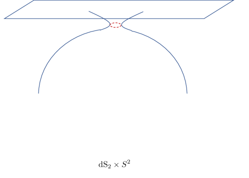
Figure 24: The late time spatial slice (such as in Fig.16 with small $R_{s}$) is Wheeler’s bag of gold made by ${\rm dS}_{2}\times S^{2}$ containing infinitely many infrared modes.

The diffeomorphisms in $x$-space leaves ${\rm dS}_{2}\times S^{2}$ invariant but changes $\alpha_{1}$. In quantum notation, the diffeomorphisms generated by $\mathcal{V}(N)=\int\mathrm{d}x\,N(x)\mathcal{C}(x)$ define operators acting on infrared states

$$\widehat{e^{i\varepsilon\mathcal{V}(N)}}|r_{0},\alpha_{0};\alpha_{1}\rangle=|r_{0},\alpha_{0};\alpha^{\prime}_{1}\rangle,\quad\alpha^{\prime}_{1}(x)=\alpha_{1}(x)+\varepsilon\alpha_{0}^{-1}N(x)+\varepsilon\partial_{x}N(x)$$ (164)

where $\varepsilon\in\mathbb{R}$ is an infinitesimal parameter. $\alpha^{\prime}_{1}(x)$ comes from the coordinate transformation $x\to x^{\prime}=x+\varepsilon N(x)$ and $\mathrm{d}\eta=e^{-\alpha_{1}-\alpha_{0}^{-1}x}\mathrm{d}x=e^{-\alpha_{1}^{\prime}-\alpha_{0}^{-1}x^{\prime}}\mathrm{d}x^{\prime}$. In the reduced phase space formulation, the diffeomorphisms are not gauge redundancy but symmetries of the theory. We find the Hilbert space $\mathcal{H}_{\rm dS_{2}\times S^{2}}$ of infrared states is a representation space of the group of 1-dimensional diffeomorphisms. The $x$-space is $S^{1}$ in ${\rm dS_{2}}\times{S^{2}}$ as $t\to\infty$. Therefore $\mathcal{H}_{\rm dS_{2}\times S^{2}}$ carries a representation of ${\rm Diff}(S^{1})$ or equivalently $\mathcal{H}_{\rm dS_{2}\times S^{2}}$ carries a representation of Witt algebra:

$$\left[L_{m},L_{n}\right]=(m-n)L_{m+n},\quad L_{n}=-ie^{in\theta}\frac{\partial}{\partial\theta},$$ (165)

or Virasoro algebra if we generally allow nontrivial central extension. $L_{n}$ as infinitesimal diffeomorphisms give infinitely many conserved charges (recall Eq.49).

11 Outlook

The analysis of this work opens new windows of developments in 3 phases of quantum black hole dynamics. These 3 phases are (1) from black hole to the Nariai limit, (2) near the Nariai limit, and (3) from the Nariai limit to white hole. The future analysis of these 3 phases needs the upgrade from the present effective dynamics to a quantum operator formulation, which is a research undergoing.

As an advantage of the reduced phase space formulation, a proper quantization of the physical Hamiltonian ${\bf H}_{\Delta}$ generates manifestly unitary time evolution. In the phase (1) from black hole to the Nariai limit, it is interesting to investigate the thermalization predicted from ${\bf H}_{\Delta}$, for instance, questions like whether we can find local observables that thermalize after the formation of the black hole, and if they relates to the Hawking radiation. A standard formalism of addressing these question is the Eigenstate Thermalization Hypothesis (ETH), whose purpose is to explain how (local) thermal equilibrium can be achieved by quantum evolutions from initially far-from-equilibrium states. A wide variety of many-body systems are shown to satisfy ETH, suggesting thermalization should be a generic feature for interacting quantum system (see e.g.Rigol_2008 ). We expect that the ${\bf H}_{\Delta}$ should lead to thermalization of certain local observables. Moreover, thermalization often combines the quantum chaos and information scrambling Srednicki_1999 which are other perspectives to be investigated. In addition, ${\bf H}_{\Delta}$ may be related to the recent studies in Liu:2020jsv on equilibrated pure states after long-time unitary evolution, in order to understand if the long-time unitary evolution of ${\bf H}_{\Delta}$ can be approximately typical and lead equilibrated pure states as outputs. The entanglement entropy of the final state might give an explain of the replica wormholes and page curves following the line of Liu:2020jsv .

In the phase (2), it is important to carry out careful analysis for the expected quantum tunneling from the viewpoint of the quantum ${\bf H}_{\Delta}$, as mentioned earlier. On the other hand, the infrared modes in the Nariai limit and the Hilbert space $\mathcal{H}_{\rm{dS}_{2}\times S^{2}}$ should be analyzed in more rigorous manner. It is interesting to describe $\mathcal{H}_{\rm{dS}_{2}\times S^{2}}$ in terms of representations of $\mathrm{Diff}(S^{1})$, and also understand the states as resulting from the unitary evolution of ${\bf H}_{\Delta}$. We may also looking for their relation with the equilibrated states. In addition, $\mathcal{H}_{\rm{dS}_{2}\times S^{2}}$ might be embedded in the language of quantum error correcting code, as the code subspace similar as in Penington:2019kki . It might also relate to states of baby universes Marolf:2020rpm . There are debates about whether the modes in the Wheeler’s bag of gold form infinitely dimensional Hilbert space, or these infrared modes inside the black hole are linearly dependent (The recent progresses from the AdS/CFT suggests that the Hilbert space may be actually 1-dimensional, see e.g. Hsin:2020mfa ). The unitary dynamics of ${\bf H}_{\Delta}$ should help to clarify the dimension of $\mathcal{H}_{\rm{dS}_{2}\times S^{2}}$ of the infrared modes.

Rigorously speaking, the existence of the phase (3) relies on the precise description of the phase (2). We expect that the Nariai geometry ${\rm dS}_{2}\times S^{2}$ is not stable at the quantum level. Its decay and relation to the white hole requires to be further analyzed in detail. It is also interesting to investigate the dynamics of the infrared modes in ${\rm dS}_{2}\times S^{2}$ toward the white hole and the asymptotically flat regime. As discussed earlier, we expect this dynamics to be highly chaotic. It is interesting to understand the chaos in the full quantum theory instead of the effective theory. The detailed analysis of the black-hole-to-white-hole transition should shed light on the resolution of information paradox, given that our discussion is based on the unitary evolution of ${\bf H}_{\Delta}$.

Another important aspect is the strong quantum dynamical regime in the blue diamond in Figure 19. The analysis may be carried by the quantization of ${\bf H}_{\Delta}$, or may require the full theory of LQG (see DAmbrosio:2020mut for a discussion based on spinfoams). We plan to apply the full theory of LQG to black holes, preferably using the new path integral formulation similar to the recent works on cosmology Han:2019vpw ; Han:2020chr ; Han:2020iwk .

References

- (1) C. G. Boehmer and K. Vandersloot, Loop Quantum Dynamics of the Schwarzschild Interior, Phys. Rev. D 76 (2007) 104030, [arXiv:0709.2129].
- (2) A. Ashtekar and M. Bojowald, Quantum geometry and the Schwarzschild singularity, Class. Quant. Grav. 23 (2006) 391–411, [gr-qc/0509075].
- (3) L. Modesto, Loop quantum black hole, Class. Quant. Grav. 23 (2006) 5587–5602, [gr-qc/0509078].
- (4) A. Ashtekar, F. Pretorius, and F. M. Ramazanoglu, Evaporation of 2-Dimensional Black Holes, Phys. Rev. D 83 (2011) 044040, [arXiv:1012.0077].
- (5) D.-W. Chiou, W.-T. Ni, and A. Tang, Loop quantization of spherically symmetric midisuperspaces and loop quantum geometry of the maximally extended Schwarzschild spacetime, arXiv:1212.1265.
- (6) R. Gambini, J. Olmedo, and J. Pullin, Quantum black holes in Loop Quantum Gravity, Class. Quant. Grav. 31 (2014) 095009, [arXiv:1310.5996].
- (7) E. Bianchi, M. Christodoulou, F. D’Ambrosio, H. M. Haggard, and C. Rovelli, White Holes as Remnants: A Surprising Scenario for the End of a Black Hole, Class. Quant. Grav. 35 (2018), no. 22 225003, [arXiv:1802.04264].
- (8) F. D’Ambrosio, M. Christodoulou, P. Martin-Dussaud, C. Rovelli, and F. Soltani, The End of a Black Hole’s Evaporation – Part I, arXiv:2009.05016.
- (9) J. Olmedo, S. Saini, and P. Singh, From black holes to white holes: a quantum gravitational, symmetric bounce, Class. Quant. Grav. 34 (2017), no. 22 225011, [arXiv:1707.07333].
- (10) A. Ashtekar, J. Olmedo, and P. Singh, Quantum extension of the Kruskal spacetime, Phys. Rev. D98 (2018), no. 12 126003, [arXiv:1806.02406].
- (11) M. Bojowald, S. Brahma, and D.-h. Yeom, Effective line elements and black-hole models in canonical loop quantum gravity, Phys. Rev. D98 (2018), no. 4 046015, [arXiv:1803.01119].
- (12) N. Bodendorfer, F. M. Mele, and J. Münch, Effective Quantum Extended Spacetime of Polymer Schwarzschild Black Hole, Class. Quant. Grav. 36 (2019), no. 19 195015, [arXiv:1902.04542].
- (13) E. Alesci, S. Bahrami, and D. Pranzetti, Quantum gravity predictions for black hole interior geometry, Phys. Lett. B 797 (2019) 134908, [arXiv:1904.12412].
- (14) M. Assanioussi, A. Dapor, and K. Liegener, Perspectives on the dynamics in a loop quantum gravity effective description of black hole interiors, Phys. Rev. D 101 (2020), no. 2 026002, [arXiv:1908.05756].
- (15) J. G. Kelly, R. Santacruz, and E. Wilson-Ewing, Black hole collapse and bounce in effective loop quantum gravity, arXiv:2006.09325.
- (16) R. Gambini, J. Olmedo, and J. Pullin, Spherically symmetric loop quantum gravity: analysis of improved dynamics, arXiv:2006.01513.
- (17) A. Ashtekar, Black Hole evaporation: A Perspective from Loop Quantum Gravity, Universe 6 (2020), no. 2 21, [arXiv:2001.08833].
- (18) M. Bojowald, Absence of singularity in loop quantum cosmology, Phys. Rev. Lett. 86 (2001) 5227–5230, [gr-qc/0102069].
- (19) A. Ashtekar, T. Pawlowski, and P. Singh, Quantum Nature of the Big Bang: Improved dynamics, Phys. Rev. D74 (2006) 084003, [gr-qc/0607039].
- (20) C. Rovelli and E. Wilson-Ewing, Why are the effective equations of loop quantum cosmology so accurate?, Phys. Rev. D 90 (2014), no. 2 023538, [arXiv:1310.8654].
- (21) R. Bousso, Charged Nariai black holes with a dilaton, Phys. Rev. D 55 (1997) 3614–3621, [gr-qc/9608053].
- (22) K. V. Kuchar and C. G. Torre, Gaussian reference fluid and interpretation of quantum geometrodynamics, Phys. Rev. D43 (1991) 419–441.
- (23) K. Giesel and T. Thiemann, Scalar Material Reference Systems and Loop Quantum Gravity, Class. Quant. Grav. 32 (2015) 135015, [arXiv:1206.3807].
- (24) K. Giesel, J. Tambornino, and T. Thiemann, LTB spacetimes in terms of Dirac observables, Class. Quant. Grav. 27 (2010) 105013, [arXiv:0906.0569].
- (25) J. Münch, Effective Quantum Dust Collapse via Surface Matching, arXiv:2010.13480.
- (26) S. Hawking and S. F. Ross, Duality between electric and magnetic black holes, Phys. Rev. D 52 (1995) 5865–5876, [hep-th/9504019].
- (27) R. Bousso, Quantum global structure of de Sitter space, Phys. Rev. D 60 (1999) 063503, [hep-th/9902183].
- (28) R. Bousso and S. W. Hawking, Pair creation and evolution of black holes in inflation, Helv. Phys. Acta 69 (1996) 261–264, [gr-qc/9608008].
- (29) C. G. Boehmer and K. Vandersloot, Stability of the Schwarzschild Interior in Loop Quantum Gravity, Phys. Rev. D 78 (2008) 067501, [arXiv:0807.3042].
- (30) C. Rovelli and F. Vidotto, Planck stars, Int. J. Mod. Phys. D 23 (2014), no. 12 1442026, [arXiv:1401.6562].
- (31) S. H. Shenker and D. Stanford, Black holes and the butterfly effect, JHEP 03 (2014) 067, [arXiv:1306.0622].
- (32) J. Maldacena, S. H. Shenker, and D. Stanford, A bound on chaos, JHEP 08 (2016) 106, [arXiv:1503.01409].
- (33) S. Holst, Barbero’s Hamiltonian derived from a generalized Hilbert-Palatini action, Phys.Rev. D53 (1996) 5966–5969, [gr-qc/9511026].
- (34) B. Dittrich, Partial and complete observables for Hamiltonian constrained systems, Gen. Rel. Grav. 39 (2007) 1891–1927, [gr-qc/0411013].
- (35) T. Thiemann, Reduced phase space quantization and Dirac observables, Class. Quant. Grav. 23 (2006) 1163–1180, [gr-qc/0411031].
- (36) K. Giesel and T. Thiemann, Algebraic quantum gravity (AQG). IV. Reduced phase space quantisation of loop quantum gravity, Class. Quant. Grav. 27 (2010) 175009, [arXiv:0711.0119].
- (37) M. Han and H. Liu, Semiclassical limit of new path integral formulation from reduced phase space loop quantum gravity, Phys. Rev. D 102 (2020), no. 2 024083, [arXiv:2005.00988].
- (38) M. Han and H. Liu, Improved -scheme effective dynamics of full loop quantum gravity, Phys. Rev. D 102 (2020), no. 6 064061, [arXiv:1912.08668].
- (39) P. Singh and E. Wilson-Ewing, Quantization ambiguities and bounds on geometric scalars in anisotropic loop quantum cosmology, Class. Quant. Grav. 31 (2014) 035010, [arXiv:1310.6728].
- (40) M. Bojowald and R. Swiderski, Spherically symmetric quantum geometry: Hamiltonian constraint, Class. Quant. Grav. 23 (2006) 2129–2154, [gr-qc/0511108].
- (41) A. Ashtekar, A. Corichi, and P. Singh, Robustness of key features of loop quantum cosmology, Phys. Rev. D 77 (2008) 024046, [arXiv:0710.3565].
- (42) M. Han. https://github.com/LQG-Florida-Atlantic-University/black-holes, 2020.
- (43) A. Ashtekar and B. Krishnan, Dynamical horizons and their properties, Phys. Rev. D 68 (2003) 104030, [gr-qc/0308033].
- (44) H. M. Haggard and C. Rovelli, Quantum-gravity effects outside the horizon spark black to white hole tunneling, Phys. Rev. D 92 (2015), no. 10 104020, [arXiv:1407.0989].
- (45) D. A. Roberts and D. Stanford, Two-dimensional conformal field theory and the butterfly effect, Phys. Rev. Lett. 115 (2015), no. 13 131603, [arXiv:1412.5123].
- (46) P. Hosur, X.-L. Qi, D. A. Roberts, and B. Yoshida, Chaos in quantum channels, JHEP 02 (2016) 004, [arXiv:1511.04021].
- (47) A. Dapor and K. Liegener, Cosmological Effective Hamiltonian from full Loop Quantum Gravity Dynamics, Phys. Lett. B785 (2018) 506–510, [arXiv:1706.09833].
- (48) R. Figari, R. Hoegh-Krohn, and C. Nappi, Interacting Relativistic Boson Fields in the de Sitter Universe with Two Space-Time Dimensions, Commun. Math. Phys. 44 (1975) 265–278.
- (49) M. Rigol, V. Dunjko, and M. Olshanii, Thermalization and its mechanism for generic isolated quantum systems, Nature 452 (Apr, 2008) 854–858.
- (50) M. Srednicki, The approach to thermal equilibrium in quantized chaotic systems, Journal of Physics A: Mathematical and General 32 (Jan, 1999) 1163–1175.
- (51) H. Liu and S. Vardhan, Entanglement entropies of equilibrated pure states in quantum many-body systems and gravity, arXiv:2008.01089.
- (52) G. Penington, S. H. Shenker, D. Stanford, and Z. Yang, Replica wormholes and the black hole interior, arXiv:1911.11977.
- (53) D. Marolf and H. Maxfield, Observations of Hawking radiation: the Page curve and baby universes, arXiv:2010.06602.
- (54) P.-S. Hsin, L. V. Iliesiu, and Z. Yang, A violation of global symmetries from replica wormholes and the fate of black hole remnants, arXiv:2011.09444.
- (55) M. Han and H. Liu, Effective Dynamics from Coherent State Path Integral of Full Loop Quantum Gravity, Phys. Rev. D101 (2020), no. 4 046003, [arXiv:1910.03763].
- (56) M. Han, H. Li, and H. Liu, Manifestly Gauge-Invariant Cosmological Perturbation Theory from Full Loop Quantum Gravity, 5, 2020. arXiv:2005.00883.