On the Secrecy Capacity of MIMO Wiretap Channels: Convex Reformulation and Efficient Numerical Methods

Abstract

This paper presents novel numerical approaches to finding the secrecy capacity of the multiple-input multiple-output (MIMO) wiretap channel subject to multiple linear transmit covariance constraints, including sum power constraint, per antenna power constraints and interference power constraint. An analytical solution to this problem is not known and existing numerical solutions suffer from slow convergence rate and/or high per-iteration complexity. Deriving computationally efficient solutions to the secrecy capacity problem is challenging since the secrecy rate is expressed as a difference of convex functions (DC) of the transmit covariance matrix, for which its convexity is only known for some special cases. In this paper we propose two low-complexity methods to compute the secrecy capacity along with a convex reformulation for degraded channels. In the first method we capitalize on the accelerated DC algorithm which requires solving a sequence of convex subproblems, for which we propose an efficient iterative algorithm where each iteration admits a closed-form solution. In the second method, we rely on the concave-convex equivalent reformulation of the secrecy capacity problem which allows us to derive the so-called partial best response algorithm to obtain an optimal solution. Notably, each iteration of the second method can also be done in closed form. The simulation results demonstrate a faster convergence rate of our methods compared to other known solutions. We carry out extensive numerical experiments to evaluate the impact of various parameters on the achieved secrecy capacity.

Index Terms - MIMO, wiretap channel, secrecy capacity, sum power constraint, per antenna power constraint, convex-concave.

I Introduction

Security has always been a great concern to the public since the very early days of wireless communications. This problem is increasingly important nowadays since wireless connectivity becomes an integral part of our modern life. Our dependency on wireless communications and the associated risks are apparent during the current global pandemic. Wireless communications offers great flexibility and convenience to manage our lives but, at the same time, also creates more entries for adversaries to attack due to its open broadcasting nature.

Primary methods for data security are traditionally based on cryptographic techniques which are mainly implemented at the higher layers (e.g the application layer) of the open systems interconnection (OSI) model of a communication network. The computational complexity of the encryption key management in cryptographic techniques is a major issue to apply them to a large number of low-cost IoT devices or in dynamic and open environments. Specifically, IoT devices are typically limited in terms of storage and computing capability to handle such complicated encryption/decryption algorithms. As a result, secure data transmission strategies based on the physical properties of radio channels have been studied as a promising alternative, which gives rise to physical layer security (PLS). Compared to conventional cryptographic methods, PLS has distinguishing advantages, including low-complexity in nature and possibly key-less secure transmission. Thus, PLS is a powerful solution to address the data security in future wireless networks, and has become a research area of growing interest in the last decade.

The PLS started with the notion of perfect secrecy by Shannon in [2]. In [3], Wyner introduced and studied the secrecy capacity of the wiretap channel (WTC) which is a fundamental information-theoretic model for PLS. In the WTC, a legitimate transmitter wishes to securely transmit data to a legitimate receiver in the presence of an eavesdropper. The secrecy capacity is simply thought as the maximum rate at which the transmitter can reliably communicate with the receiver while ensuring that the eavesdropper cannot decode the information. Since Wyner’s seminal paper, the WTC has been extended, covering various scenarios. In particular, the secrecy capacity of the Gaussian WTC was studied [4]. The use of multiple antennas at transceivers in contemporary wireless communications systems gives rise to the so-called multiple-input multiple-output (MIMO) Gaussian WTC. The secrecy capacity of the MIMO Gaussian WTC has received significant interest since the late 2000s. In this regard, there have been many results in the literature and we attempt to comprehensively (but by no means exhaustively) summarize the significant ones below.

An analytical solution for the multiple-input single-output (MISO) Gaussian WTC where both the eavesdropper and the legitimate receiver have a single antenna was proposed in [5]. When the channel state information is perfectly known, the secrecy capacity of MIMO WTC was characterized in [6, 7, 8]. Particularly, explicit expressions for optimal signaling for MIMO WTC are possible under some special cases [9, 10, 11]. For example, in [10] Fakoorian et.al presented a full-rank solution for Gaussian MIMO WTC under an average power constraint. A closed-form solution for optimal signaling for strictly degraded Gaussian MIMO WTC with sufficiently large power was presented in [11]. In [12] the secrecy rate maximization problem for the MIMO WTC with multiple eavesdroppers was considered, in which an alternating matrix based algorithm, named polynomial time difference of convex functions (POTDC), was introduced. Power minimization and secrecy rate maximization for the MIMO WTC was studied in [13] using a difference of convex functions algorithm (DCA). More recently, an efficient low-complex solution for the MIMO WTC was proposed in [14] using a convex-concave optimization framework. We note that the above studies on MIMO wiretap channels focused on the secrecy capacity subject to a sum power constraint (SPC).

In a MIMO communications system, each transmit antenna can be equipped with a separate RF chain, and thus a per-antenna power constraint (PAPC) is more practically relevant than constraining the sum power [15],[16]. In this regard, the secrecy capacity with joint SPC and PAPC has been studied in [17, 18] for the Gaussian MIMO WTC, and more recently in [19] for the MISO Gaussian WTC. More specifically, an iterative algorithm that combines the alternating optimization (AO) method and the subgradient method to compute the secrecy capacity of the MIMO WTC for joint SPC and PAPC was proposed in [17]. Based on an equivalent minimax reformulation of the secrecy capacity problem, a barrier method was presented in [18]. Very recently, a closed-form solution of optimal transmit strategies for Gaussian MISO wiretap channels were derived in [19]. In [20, 21], the Gaussian MIMO WTC was extended to scenarios where the transmitter also needs to limit its interference below a threshold. We refer to this kind of constraint as an interference power constraint (IPC).

In this paper we consider the problem of finding the secrecy capacity-achieving input covariance for Gaussian MIMO wiretap channels with joint SPC, PAPC, and IPC. As mentioned above, analytical solutions to the general Gaussian MIMO WTC have not been reported, and thus efficient numerical methods are desired. To this end we note that the solution proposed in [17] suffers a slow convergence rate which is inherent in subgradient methods. In addition, this method can only yield a locally optimal solution. On the contrary, the barrier method presented in [18], being a Newton-type method, converges very fast but its per-iteration complexity increases rapidly with the problem size. Thus, our motivation is to develop more efficient numerical methods to solve the secrecy capacity problem of the MIMO WTC. To this end we propose two algorithms which can overcome the shortcomings of these existing solutions. Although, new research directions in the study of the MIMO WTC are not the scope of this paper, the proposed numerical methods are still of significant importance since they will help find the capacity and optimal signaling faster, which is useful to deal with time-varying channels. For example, in a closed-loop system, we need to solve the secrecy problem whenever the channels are updated. In this regard, the secrecy optimization problem is an on-line task. As a result, our proposed fast converging algorithms are always desired, and thus, will certainly create an impact. Our main contributions are as follows:

• For the degraded Gaussian MIMO WTC, we present a convex reformulation for finding the optimal signaling and the secrecy capacity. We remark that in this case, the secrecy capacity problem is in fact convex but is expressed in a non-convex form. To our knowledge, no convex reformulation has been reported for a general set up as considered in this paper. The convex reformulation allows us to solve the secrecy capacity problem using off-the-shelf convex solvers for different types of transmit power constraints for which analytical solutions are impossible.

• For the general Gaussian MIMO WTC, we apply an accelerated DCA [22] to solve the secrecy capacity problem, which requires solving a sequence of convex subproblems. To solve these subproblems, we customize the CoMirror algorithm introduced in [23] to achieve an iterative method where each iteration is solved in closed-form. The numerical results demonstrate that the accelerated DCA converges very much quicker, compared to a known solution that is based on AO.

• For the general Gaussian MIMO WTC, we also propose an efficient iterative method to calculate the secrecy capacity, which is based on the equivalent concave-convex reformulation of the secrecy capacity problem. We refer to this proposed method as the partial best response algorithm (PBRA). The idea of PBRA is to find a saddle point of the concave-convex game, by optimizing one variable while the other is held fixed. The novelty of the PBRA is the use of a proper approximation of the saddle-point objective to achieve monotonic convergence to a saddle point. Also, each iteration of the PBRA can be solved efficiently.

Notation: We use bold uppercase and lowercase letters to denote matrices and vectors, respectively. $\mathbb{C}^{M\times N}$ denotes the space of $M\times N$ complex matrices. To lighten the notation, $\mathbf{I}$ and $\mathbf{0}$ define identity and zero matrices respectively, of which the size can be easily inferred from the context. $||\cdot||_{F}$ and $||\cdot||_{1}$ denote the Frobenius and $\ell_{1}$ norm. $\mathbf{H}^{{\dagger}}$ and $\mathbf{H}^{\mathsf{T}}$ are Hermitian and ordinary transpose of $\mathbf{H}$, respectively; $\mathbf{H}_{i,j}$ is the $(i,j)$-entry of $\mathbf{H}$; $|\mathbf{H}|$ is the determinant of $\mathbf{H}$; Furthermore, we denote the expected value of a random variable by $E\{.\}$, and $[x]_{+}=\max(x,0)$. The $i$th unit vector (i.e., its $i$th entry is equal to one and all other entries are zero) is denoted by $\mathbf{e}_{i}$. The notation $\mathbf{A}\succeq(\succ)\mathbf{B}$ means $\mathbf{A}-\mathbf{B}$ is positive semidefinite (definite). $\nabla_{\mathbf{X}}f$, where $\mathbf{X}\in\mathbb{C}^{M\times N}$, denotes the complex gradient with respect to $\mathbf{X}^{\ast}$ as defined in [24]. $P_{\mathcal{C}}(\mathbf{x})$ is the Euclidean projection of $\mathbf{x}$ onto the set $\mathcal{C}$. $\mathcal{CN}(\mathbf{0},\mathbf{A})$ denotes a circularly-symmetric complex-valued Gaussian random vector with zero mean and covariance $\mathbf{A}$

II System Model

Consider a MIMO WTC with a transmitter (Alice), a legitimate receiver (Bob) and an eavesdropper (Eve). Let $N_{t}$, $N_{r}$, and$N_{e}$ denote the number of antennas at Alice, Bob, and Eve, respectively. The signals received at Bob and Eve can be expressed as

$$\mathbf{y}_{b} =\mathbf{H}_{b}\mathbf{x}+\mathbf{z}_{r}$$ (1a)

$$\mathbf{y}_{e} =\mathbf{H}_{e}\mathbf{x}+\mathbf{z}_{e}$$ (1b)

respectively. In the equation above, $\mathbf{x}$ is the confidential signal that Alice wishes to transmit to Bob, while keeping it secret from Eve; $\mathbf{H}_{b}\in\mathbb{C}^{N_{r}\times N_{t}}$ and $\mathbf{H}_{e}\in\mathbb{C}^{N_{e}\times N_{t}}$ are the complex channel matrix between Alice and Bob, and between Alice a and Eve. $\mathbf{z}_{r}\in\mathbb{C}^{N_{r}\times 1}\sim\mathcal{CN}(\mathbf{0},\mathbf{I})$ and $\mathbf{z}_{e}\in\mathbb{C}^{N_{e}\times 1}\sim\mathcal{CN}(\mathbf{0},\mathbf{I})$ are additive white Gaussian noise at the legitimate receiver and at the eavesdropper respectively. In this paper $\mathbf{H}_{b}$ and $\mathbf{H}_{e}$ are assumed to be quasi-static and perfectly known at all nodes. For a given input covariance matrix $\mathbf{X}=E\{\mathbf{x}\mathbf{x}^{{\dagger}}\}\succeq\mathbf{0}$, where $E\{\cdot\}$ is the statistical expectation, the maximum secrecy rate (in nat/s/Hz) between Alice and Bob is given by [8]

$$C_{s}(\mathbf{X})=\left[\underbrace{\ln|\mathbf{I}+\mathbf{H}_{b}\mathbf{X}\mathbf{H}_{b}^{{\dagger}}|}_{f_{b}(\mathbf{X})}-\underbrace{\ln|\mathbf{I}+\mathbf{H}_{e}\mathbf{X}\mathbf{H}_{e}^{{\dagger}}|}_{f_{e}(\mathbf{X})}\right]_{+}.$$ (2)

In this paper we are interested in the secrecy capacity of MIMO WTC subject to some constraints on the transmit covariance, which is mathematically stated as

$$\boxed{C_{s}\triangleq\underset{\mathbf{X}\in\mathcal{X}}{\max}\ C_{s}(\mathbf{X})}$$ (3)

where $\mathcal{X}$ is determined by the transmit power constraints of interest. Some typical examples of $\mathcal{X}$ are given below.

• The SPC:

  $$\mathcal{X}_{\textrm{spc}}=\left\{\mathbf{X}\succeq\mathbf{0}\ |\ \operatorname{tr}(\mathbf{X})\leq P_{0}\right\}$$ (4)

  where $P_{0}$ is the total power budget. This setting is fundamental to MIMO WTC and its secrecy capacity has been extensively studied [7, 8, 10, 11, 14]. In this case the SPC can be set to $\operatorname{tr}(\mathbf{X})=P_{0}$ without loss of optimality.

• The PAPC:

  $$\mathcal{X}_{\textrm{papc}}=\left\{\mathbf{X}\succeq\mathbf{0}\ |\ [\mathbf{X}]_{i,i}\leq P_{i},i=1,2,\dots,N_{t}\right\}$$ (5)

  where $P_{i}$ is the maximum allowed power for the $i$-th antenna. It very often that joint SPC and PAPC (i.e. $\mathcal{X}=\mathcal{X}_{\textrm{spc}}\cap\mathcal{X}_{\textrm{papc}})$ is considered in the literature, e.g., in [17, 25] for MIMO WTC and recently in [19] for MISO WTC.

• The interference power constraint (IPC):

  $$\mathcal{X}_{\textrm{ipc}}=\left\{\mathbf{X}\succeq\mathbf{0}\ |\ \operatorname{tr}(\mathbf{W}_{l}\mathbf{X})\leq P_{l},l=1,2,\ldots,N_{p}\right\}$$ (6)

  where $\mathbf{W}_{l}=\mathbf{H}_{l}^{{\dagger}}\mathbf{H}_{l}$ and $\mathbf{H}_{l}$ is the channel between Alice and the $l$-th primary receiver, $P_{l}\geq 0$ is the corresponding interference threshold, and $N_{p}$ is the number of primary receivers. It means that the interference energy from Alice to the $l$-th primary receiver should be limited by a predetermined threshold. The case for $\mathcal{X}=\mathcal{X}_{\textrm{spc}}\cap\mathcal{X}_{\textrm{ipc}}$was studied in [21, 20].

We remark that $C_{s}>0$ if and only if $\mathbf{H}_{b}^{{\dagger}}\mathbf{H}_{b}-\mathbf{H}_{e}^{{\dagger}}\mathbf{H}_{e}$ is positive semidefinite or indefinite, i.e. $\mathbf{H}_{b}^{{\dagger}}\mathbf{H}_{b}-\mathbf{H}_{e}^{{\dagger}}\mathbf{H}_{e}$ has at least one positive eigenvalue, which is assumed in the sequel of the paper. A proof for this can be found in [26, Appendix A]. Thus we can remove the max operator in (3) onward without loss of optimality. Further, let $\mathbf{X}^{\ast}$ be the optimal input covariance matrix of (3). Then it was proved in [7, Corollary 1] that the secrecy capacity can be achieved by a wiretap coding scheme the follows a circularly-symmetric complex-valued Gaussian random vector with zero mean and covariance $\mathbf{X}^{\ast}$. Moreover, for a given $\mathbf{X}^{\ast}$, a way to construct a Gaussian wiretap code that achieves the secrecy capacity was presented in [27]. The idea is to apply the generalized singular value decomposition to decompose the MIMO wiretap channel into several parallel eigen-subchannels. Then, to achieve the secrecy capacity, Gaussian wiretap codebooks are sent along the subchannels where the gains to Bob are larger than those to Eve. We refer the interested readers to [27] for further details. One may argue that considering capacity achieving schemes as done in this paper is not of practical importance since discrete modulation schemes and coding rates are used in practice. However, we note that solving (3) is still practically meaningful. Firstly, it can give an upper bound on what we can achieve in terms of secrecy rate. Secondly, the obtained optimal covariance matrix can be useful to construct wiretap codes with practical finite-alphabet input that can achieve a secrecy rate close to the secrecy capacity up to an SNR threshold [28].

III Convex Reformulations for MIMO Wiretap Channels

III-A The Degraded Case

In general $C_{s}(\mathbf{X})$ is non-convex with respect to $\mathbf{X}$, and thus, finding optimal signaling for MIMO WTC is difficult. However, if the channel is degraded (i.e. $\mathbf{H}_{b}^{{\dagger}}\mathbf{H}_{b}\succeq\mathbf{H}_{e}^{{\dagger}}\mathbf{H}_{e}$) then $C_{s}(\mathbf{X})$ becomes concave (i.e. problem (3) is convex) [8], and thus, efficient algorithms for solving (3) are possible in principle. More specifically, analytical solutions have been reported for degraded MIMO WTC under some specific power constraints. For example, full-rank solutions via water-filling like algorithm for the SPC only was presented in [10]. Moreover, when the transmit power is sufficient large, closed-form for optimal signaling is possible [11]. When $\mathcal{X}$ is either SPC only or PAPC only, closed-form solutions are presented in [19] for MISO WTC. When $\mathcal{X}$ stands for the joint SPC and PAPC, numerical solutions based on alternating optimization are proposed in [17] for MIMO WTC.

Regarding numerical algorithms for finding optimal signaling for degraded MIMO WTC, we note that off-the-shelf convex solvers cannot be used to solve (3) directly despite its convexity, since it is not expressed in a standard convex form. To overcome this issue, one could customize standard algorithms for convex optimization such as interior-point methods or gradient based methods to solve (3), which was done e.g. in [18].In this section, we equivalently reformulate (3) as a standard convex problem for degraded MIMO WTC. As a result, we can avail of powerful modern convex solvers to compute the optimal signaling. In this regard, the following lemma is in order.

Lemma 1.

Let $\boldsymbol{\Delta}=\mathbf{H}_{b}^{{\dagger}}\mathbf{H}_{b}-\mathbf{H}_{e}^{{\dagger}}\mathbf{H}_{e}\succeq\mathbf{0}$. Then problem (3) is equivalent to the following convex problem

$$\underset{\mathbf{X}\succeq\mathbf{0},\mathbf{Y}\succeq\mathbf{0}}{\mathrm{maximize}} \ \ln|\mathbf{Y}|$$ (7a)

$$\operatorname{subject~{}to} \ \begin{bmatrix}\mathbf{I}+\boldsymbol{\Delta}^{1/2}\mathbf{X}\boldsymbol{\Delta}^{1/2}-\mathbf{Y}&\boldsymbol{\Delta}^{1/2}\mathbf{X}\mathbf{H}_{e}^{{\dagger}}\\ \mathbf{H}_{e}\mathbf{X}\boldsymbol{\Delta}^{1/2}&\mathbf{I}+\mathbf{H}_{e}\mathbf{X}\mathbf{H}_{e}^{{\dagger}}\end{bmatrix}\succeq\mathbf{0}$$ (7b)

$$\ \mathbf{X}\in\mathcal{X}$$ (7c)

where $$\mathcal{X}$$ denotes any convex set of transmit covariance constraints including those in (4), (5), (6), or any combination thereof.

Proof:

Please refer to Appendix 1. ∎

We note that a similar convex reformulation was also presented for degraded channels in [29] for the SPC and Alice also sends some power to an energy harvester which acts as an eavesdropper. The proof in [29] is quite involved. In our paper, we only require the feasible set of the secrecy capacity problem to be convex. Thus, it can deal with any linear transmit covariance matrix constraints, including energy harvesting threshold constraint as a special case. We remark that our proof for the convex reformulation is based on the epigraph form of (3) and is much more elegant. We further remark that (7) can be converted into a standard semidefinite program, which is done automatically by modeling tools for convex optimization such as CVX [30] and YALMIP [31]. The interested reader is referred to [32, p. 149] for further details. To conclude this section we note that modern off-the-shelf solvers such as MOSEK [33] can solve (7) very fast when $N_{t}$ is not too large.

III-B The General Case

For nondegraded MIMO WTC, problem (3) is a non-convex program in general, and thus, finding optimal signaling is difficult. In such cases, a convex-concave reformulation of (3) is particularly useful. Specifically, based on the collective results in [34, 8, 7, 18, 20], the secrecy capacity of general MIMO WTC in (3) can be equivalently expressed in the form of a minimax optimization problem as

$$\boxed{C_{s}=\underset{\mathbf{K}\in\mathcal{K}}{\min}\ \underset{\mathbf{X}\in\mathcal{X}}{\max}\ f(\mathbf{K},\mathbf{X})\triangleq\log\frac{|\mathbf{I}+\mathbf{K}^{-1}\mathbf{H}\mathbf{X}\mathbf{H}^{{\dagger}}|}{|\mathbf{I}+\mathbf{H}_{e}\mathbf{X}\mathbf{H}_{e}^{{\dagger}}|}}$$ (8)

where $\mathbf{H}=[\mathbf{H}_{b}^{\mathsf{T}},\mathbf{H}_{e}^{\mathsf{T}}]^{\mathsf{T}}\in\mathbb{C}^{(N_{r}+N_{e})\times N_{t}}$ is the extended channel, $\mathcal{X}$ stands for the transmit power constraints including SPC, PAPC and IPC, or any combination thereof, and $\mathcal{K}$ is defined as

$$\mathcal{K}=\left\{\mathbf{K}\left|\mathbf{K}=\small\left[\begin{array}[]{cc}\mathbf{I}&\bar{\mathbf{K}}\\ \bar{\mathbf{K}}^{{\dagger}}&\mathbf{I}\end{array}\right];\bar{\mathbf{K}}\in\mathbb{C}^{N_{r}\times N_{e}};\mathbf{K}\succeq\mathbf{0}\right.\right\}.$$ (9)

The set $\mathcal{K}$ deserves further explanations. In fact, $\mathbf{K}$ in (8) is the covariance matrix of the following composite noise:

$$\mathbf{z}=\begin{bmatrix}\mathbf{z}_{r}\\ \mathbf{z}_{e}\end{bmatrix}$$ (10)

which is obtained by assuming that Bob knows both $\mathbf{H}_{b}$ and $\mathbf{H}_{e}$ [7, 8]. As a result, $\mathbf{K}$ is defined as

$$\mathbf{K}=\left[\begin{array}[]{cc}E\bigl{\{}\mathbf{z}_{r}\mathbf{z}_{r}^{{\dagger}}\bigr{\}}&E\bigl{\{}\mathbf{z}_{r}\mathbf{z}_{e}^{{\dagger}}\bigr{\}}\\ E\bigl{\{}\mathbf{z}_{e}\mathbf{z}_{r}^{{\dagger}}\bigr{\}}&E\bigl{\{}\mathbf{z}_{e}\mathbf{z}_{e}^{{\dagger}}\bigr{\}}\end{array}\right]=\left[\begin{array}[]{cc}\mathbf{I}&\bar{\mathbf{K}}\\ \bar{\mathbf{K}}^{{\dagger}}&\mathbf{I}\end{array}\right],$$

where $\bar{\mathbf{K}}$ represents the correlation between $\mathbf{z}_{r}$ and $\mathbf{z}_{e}$.

We remark that (8) is true regardless of the degradedness of the MIMO WTC. The significance of the above minimax reformulation is two fold. First, computing the secrecy capacity is always equivalent to finding a saddle point of (8). Second, (8) is more numerically tractable since $f(\mathbf{K},\mathbf{X})$ is convex with respect to $\mathbf{K}$ and is concave with respect to $\mathbf{X}$. Thus, (8) is also widely known as a convex-concave problem. Let $(\mathbf{X}^{\ast},\mathbf{K}^{\ast})$ be the saddle point of (8) which always exists since $\mathcal{X}$ and $\mathcal{K}$ are convex and compact. Then the following inequality holds

$$f(\mathbf{X},\mathbf{K}^{\ast})\leq C_{s}=f(\mathbf{X}^{\ast},\mathbf{K}^{\ast})\leq f(\mathbf{X}^{\ast},\mathbf{K}).$$ (11)

Further $f(\mathbf{K},\mathbf{X})$ is an upper bound of $C_{s}(\mathbf{X})$, i.e. $f(\mathbf{K},\mathbf{X})\geq C_{s}(\mathbf{X})$ for any feasible $(\mathbf{K},\mathbf{X})$. However, it is worth noting that, while the equality $\underset{\mathbf{K}\in\mathcal{K}}{\min}\ \underset{\mathbf{X}\in\mathcal{X}}{\max}\ f(\mathbf{K},\mathbf{X})=\underset{\mathbf{X}\in\mathcal{X}}{\max}\ C_{s}(\mathbf{X})$ is always true, a saddle point $(\mathbf{X}^{\ast},\mathbf{K}^{\ast})$ to (8) is not necessarily an optimal solution to (3) in general. More precisely, it is possible that $C_{s}=f(\mathbf{X}^{\ast},\mathbf{K}^{\ast})>C_{s}(\mathbf{X}^{\ast})$ for some cases, especially when (8) has multiple saddle points. For example, consider the following real-valued channel matrices for simplicity:

$$\mathbf{H}_{b}=\begin{bmatrix}-0.4176&1.4224\\ -1.4963&-2.0426\end{bmatrix};\mathbf{H}_{e}=\begin{bmatrix}0.6726&1.4335\\ 1.7762&-0.3694\end{bmatrix}.$$ (12)

Note that the resulting MIMO WTC is nondegraded and thus convex reformulation presented in the preceding subsection is not applicable. For the joint SPC and PAPC given in (5) with $P_{0}=10$, $P_{1}=P_{2}=6$, solving (8) (using the minimax barrier method in [18] or Algorithm 3 presented shortly) yields

$$\mathbf{X}^{\ast}=\begin{bmatrix}1.7305&1.2198\\ 1.2198&5.9985\end{bmatrix}\ \textrm{and}\ C_{s}=1.0420,$$ (13)

but $C_{s}(\mathbf{X}^{\ast})=0.3409<C_{s}$. However, if the SPC is active, i.e. $\operatorname{tr}(\mathbf{X}^{\ast})=P_{0}$, then $\mathbf{X}^{\ast}$ is also a maximizer of (3). The above example implies that numerical algorithms for solving both (3) and (8) are desired.

To motivate the efficient numerical methods proposed in the subsequent sections we note that existing numerical solutions for solving (3) for general MIMO WTC can be generally classified into two ways. The first one is based on local optimization approaches to solving (3) directly with the hope that they can also yield an optimal solution by a good initialization [17, 25, 35]. The drawback of such methods is that the achieved covariance matrix is not guaranteed to be the optimal signaling. The second way is based on finding a saddle point of a convex-concave reformulation of (3) [18]. However, as explained by the example above, such a method always gives the secrecy capacity but not necessarily the optimal signaling. More explicitly, if we construct a Gaussian wiretap code based on the obtained saddle point of (8), then the achievable secrecy rate can be strictly smaller than the secrecy capacity.

III-C A Suboptimal Method

For comparison purpose we briefly describe a suboptimal method that can efficiently compute an achievable secrecy rate. In particular, this method is obtained by forcing $\mathbf{H}_{e}\mathbf{X}\mathbf{H}_{e}^{{\dagger}}=0$. Note that we can rewrite $\mathbf{X}=\mathbf{U}\mathbf{U}^{{\dagger}}$ for some $\mathbf{U}$. Thus the constraint $\mathbf{H}_{e}\mathbf{X}\mathbf{H}_{e}^{{\dagger}}=\mathbf{0}$ is equivalent to $\mathbf{H}_{e}\mathbf{U}=\mathbf{0}$, which means $\mathbf{\mathbf{U}}$ should belong to the null space of $\mathbf{H}_{e}$. Let $\mathbf{V}$ be a basis of the null space of $\mathbf{H}_{e}$ which is nonempty when $N_{t}>N_{e}$. Then we can write $\mathbf{X}=\mathbf{V}\mathbf{T}\mathbf{V}^{{\dagger}}$, where $\mathbf{T}\succeq\mathbf{0}$ is the solution to the following optimization problem

$$\underset{\mathbf{T}\succeq\mathbf{0}}{\operatorname{maximize}} \;\ln|\mathbf{I}+\mathbf{H}_{b}\mathbf{V}\mathbf{T}\mathbf{V}^{{\dagger}}\mathbf{H}_{b}^{{\dagger}}|$$ (14a)

$$\operatorname{subject~{}to} \mathbf{\;}\mathbf{V}\mathbf{T}\mathbf{V}^{{\dagger}}\in\mathcal{X}.$$ (14b)

In the remainder of the paper we refer to this suboptimal method as the zero-forcing (ZF) method since the idea in fact comes from the zero-forcing method for downlink multiuser MIMO [36].

IV Accelerated DCA Method for Solving (3)

IV-A Algorithm Description

As mentioned above, since the equivalent convex-concave formulation is not always useful to find the optimal signaling of the general MIMO WTC, one still needs to solve (3) directly. In [17, 25], an AO method was introduced to solve (3). Here we propose a simple but efficient method derived based on the obvious observation that $C_{s}(\mathbf{X})$ is a DC function. Note that $f_{b}(\mathbf{X})$ and $f_{e}(\mathbf{X})$ are indeed concave functions [37, Section 3.1] and $C_{s}(\mathbf{X})$ can be rewritten as $C_{s}(\mathbf{X})=-f_{e}(\mathbf{X})-(-f_{b}(\mathbf{X}))$ which is a DC function. This naturally motivates the use of DCA to solve (3). In this regard maximizing a concave function is a convex problem, and thus, the term $-f_{e}(\mathbf{X})$ is considered as the non-convex term. Thus, the main idea of the conventional DCA is to linearize the non-convex term of the problem, which is $-f_{e}(\mathbf{X})$ in our case, at a given operating point and solve the approximate convex subproblem. This process is repeated until some stopping criterion is met.

In this paper we consider an accelerated version of DCA (ADCA) presented in [22]. The idea is that from the current and previous iterates denoted by $\mathbf{X}_{n}$ and $\mathbf{X}_{n-1}$ respectively, we compute an extrapolated point $\mathbf{Z}_{n}$ using the Nesterov’s acceleration technique: $\mathbf{X}_{n}+(t_{k}-1)/t_{k+1}\bigl{(}\mathbf{X}_{n}-\mathbf{X}_{n-1}\bigr{)}$. Since $C_{s}(\mathbf{X})$ is possibly non-convex for a general MIMO WTC, $\mathbf{Z}_{n}$ can be a bad extrapolation and a monitor is required. Specifically, if $\mathbf{Z}_{n}$ is better than one of the last $q$ iterates, then $\mathbf{Z}_{n}$ is considered a good extrapolation and thus will be used instead of $\mathbf{X}_{n}$ to generate the next iterate. Thus, the ADCA is generally non-monotone. The algorithmic description of ADCA for solving (3) is outlined in Algorithm 1. Note that the subproblem in (15) is achieved by linearizing $f_{e}(\mathbf{X})$ around $\mathbf{V}_{n}$ and omitting the associated constants that do not affect the optimization. In Algorithm 1, $q$ is any non-negative integer and $\gamma_{n}$ is the minimum of the secrecy rate of the last $q$ iterates. We remark that the case when $q=0$ reduces to the conventional DCA, which is exactly the same as the AO method in [17].

Algorithm 1 ADCA for solving (3)

1:  Initialization: $\mathbf{V}_{0}=\mathbf{X}_{0}\in\mathcal{X}$, $t=\frac{1+\sqrt{5}}{2}$, $q$: integer.

2:  for  $n=1,2,\dots$ do

3:     Update:

$$\mathbf{X}_{n}=\underset{\mathbf{X}\in\mathcal{X}}{\arg\max}\ \underbrace{f_{b}(\mathbf{X})-\operatorname{tr}\bigl{(}\nabla f_{e}(\mathbf{V}_{n-1})\mathbf{X}\bigr{)}}_{\bar{f}(\mathbf{X};\mathbf{V}_{n-1})}$$ (15)

where $\nabla f_{e}(\mathbf{X})=\mathbf{H}_{e}^{{\dagger}}\bigl{(}\mathbf{I}+\mathbf{H}_{e}\mathbf{X}\mathbf{H}_{e}^{{\dagger}}\bigr{)}^{-1}\mathbf{H}_{e}$

4:     $t_{n+1}=\frac{1+\sqrt{1+4t_{n}^{2}}}{2}$

5:     $\mathbf{Z}_{n}=\mathbf{X}_{n}+\frac{t_{n}-1}{t_{n+1}}\bigl{(}\mathbf{X}_{n}-\mathbf{X}_{n-1}\bigr{)}$

6:     $\gamma_{n}=\min\bigl{(}C_{s}(\mathbf{X}_{n}),C_{s}(\mathbf{X}_{n-1}),\ldots,C(\mathbf{X}_{[n-q]_{+}})\bigr{)}$

7:     $\mathbf{V}_{n}=\begin{cases}\mathbf{Z}_{n}&\textrm{if}\ C_{s}(\mathbf{Z}_{n})\geq\gamma_{n}\\ \mathbf{X}_{n}&\textrm{otherwise}\end{cases}$

8:  end for

9:  Output: $\mathbf{X}_{n}$

Before proceeding further we also note that Algorithm 1 in our paper is not a traditional first-order Taylor method. In particular, we apply an extrapolated point which is numerically shown to improve the convergence rate.

IV-B Convergence Analysis

The convergence analysis of the ADCA is studied in [22] where the involved functions are assumed to be strongly convex. In the considered problem, this assumption does not hold for $f_{b}(\mathbf{X})$ and $f_{e}(\mathbf{X})$ in general. A weaker convergence is stated in the following lemma.

Lemma 2.

Let $\{\gamma_{n}\}$ be the sequence generated by Step 6 of Algorithm 1. Then it holds that $\gamma_{n+q}\geq\gamma_{n-1}$. If the objective $\bar{f}(\mathbf{X};\mathbf{V}_{n-1})$ is strictly concave. e.g. when $\mathbf{H}_{b}^{{\dagger}}\mathbf{H}_{b}$ is invertible, then, every limit points of Algorithm 1 is a critical point of 3.

Proof:

Please refer to Appendix -B. ∎

IV-C Solving the Subproblem for joint SPC and PAPC: CoMirror Algorithm

To implement Algorithm 1, we need to solve (15) efficiently. We remark that for the case of SPC only, waterfilling-like solution to (15) is possible. We skip the details here for the sake of brevity. Thus we focus on the joint SPC and PAPC case, i.e. $\mathcal{X}=\mathcal{X}_{\textrm{spc}}\cap\mathcal{X}_{\textrm{papc}}$ where $\mathcal{X}_{\textrm{spc}}$ and $\mathcal{X}_{\textrm{papc}}$ are defined in (4) and (5), respectively. Since (15) is a convex program, convex solvers can be used to solve it. However, the incurred complexity (including the memory requirement) is very high when $N_{t}$ is large, which is the case for massive MIMO. Our goal in this section is to derive a more efficient method for solving (15). To this end we note that the spectrahedron $\mathcal{X}_{\textrm{spc}}$ is simple in the sense that the projection onto it can be computed efficiently as shall be seen shortly. To exploit this fact, we resort to the CoMirror algorithm presented in [23] to solve (15).

To simplify the notation we will ignore $\mathbf{V}_{n-1}$ and write $\bar{f}(\mathbf{X})$ instead of $\bar{f}(\mathbf{X};\mathbf{V}_{n-1})$ onward. Let $g_{i}(\mathbf{X})=[\mathbf{X}]_{i,i}-P_{i}$. Then (15) is equivalent to

$$\underset{\mathbf{X}\in\mathcal{X}_{\textrm{spc}}}{\operatorname{maximize}} \quad\bar{f}(\mathbf{X})$$ (16a)

$$\operatorname{subject~{}to} \quad g_{i}(\mathbf{X})\leq 0,i=1,2,\ldots,N_{t}$$ (16b)

The operation of the CoMirror algorithm is as follows. For a given iterate $\mathbf{X}^{k}$, if the constraint (16b) is satisfied, then we move along the direction $\nabla\bar{f}_{t}(\mathbf{X})$ with a step size $\eta_{k}$ to maximize the objective, generating the next iterate. If (16b) is violated, set $m=\underset{1\leq i\leq N_{t}}{\arg\max}\;g_{i}(\mathbf{X})$ and move along $-\nabla g_{m}(\mathbf{X})=-\operatorname{diag}(\mathbf{e}_{m})$ to reduce $g_{m}(\mathbf{X})$, hoping to achieve a feasible solution in the next iteration. The CoMirror algorithm for solving (15) is summarized in Algorithm 2. The convergence of Algorithm 2 and other relevant discussions are provided in Appendix -C.

Algorithm 2 CoMirror algorithm for solving (15)

1:  Initialization: $\mathbf{X}^{0}\in\mathcal{X}_{\textrm{spc}}$; $\Omega=\frac{1}{\sqrt{2}}\underset{\mathbf{X}\in\mathcal{X}_{\textrm{spc}}}{\max}\ \bigl{\|}\mathbf{X}-\mathbf{X}^{0}\bigr{\|}$;

2:  for  $k=1,2\dots$ do

3:     $\mathbf{X}^{k}=P_{\mathcal{X}_{\textrm{spc}}}\left(\mathbf{X}^{k-1}+\eta_{k}\mathbf{E}_{k-1}\right)$ where

$$\mathbf{E}_{k-1}=\begin{cases}\nabla\bar{f}(\mathbf{X}_{k-1})&\underset{i=1,2,\dots,N_{t}}{\max}\{g_{i}(\mathbf{X}_{k-1})\}\leq 0\\ -\operatorname{diag}(\mathbf{e}_{m})&\textrm{otherwise}\end{cases}$$

and

$$\eta_{k}=\frac{\Omega}{\bigl{\|}\mathbf{E}_{k-1}\bigr{\|}\sqrt{k}}$$

4:  end for

5:  Output: $\mathbf{X}_{k}$

The following remarks are in order regarding the implementation of Algorithm 2. First, in this paper we use the complex gradient of $\bar{f}(\mathbf{X}_{k-1})$ defined in [24] and thus $\nabla\bar{f}(\mathbf{X}_{k-1})$ is given by

$$\nabla\bar{f}(\mathbf{X}_{k-1})=\mathbf{H}_{b}^{{\dagger}}(\mathbf{I}+\mathbf{H}_{b}\mathbf{X}_{k-1}\mathbf{H}_{b}^{{\dagger}})^{-1}\mathbf{H}_{b}-\boldsymbol{\Gamma}_{n-1}.$$

Second, for a given point $\bar{\mathbf{X}}$, the projection $P_{\mathcal{X}_{\textrm{spc}}}(\bar{\mathbf{X}})$ is mathematically stated as

$$\underset{\mathbf{X}\succeq\mathbf{0}}{\operatorname{maximize}} \quad\bigl{\|}\mathbf{X}-\bar{\mathbf{X}}\bigr{\|}_{F}^{2}$$ (17)

$$\quad\operatorname{tr}(\mathbf{X})\leq P_{0}.$$ (18)

Let $\bar{\mathbf{X}}=\mathbf{U}\operatorname{diag}(\bar{\boldsymbol{\sigma}})\mathbf{U}^{{\dagger}}$ be the eigenvalue decomposition of $\bar{\mathbf{X}}$ and $\bar{\boldsymbol{\sigma}}\in\mathbb{R}^{N_{t}}$ is the vector of the eigenvalues of $\bar{\mathbf{X}}$. Further, let $\bar{\boldsymbol{\sigma}}_{+}=\max(\bar{\boldsymbol{\sigma}},0)$. Then the solution to the above problem is given by

$$\mathbf{X}=\mathbf{U}\operatorname{diag}(P_{\Delta}(\bar{\boldsymbol{\sigma}}_{+}))\mathbf{U}^{{\dagger}}$$ (19)

where $\Delta$ denotes the full simplex is defined as

$$\Delta=\{\mathbf{t}\in\mathbb{R}^{N_{t}}|\sum\nolimits_{i=0}^{N_{t}}t_{i}\leq P_{0},t_{i}\geq 0,\forall i=1,2,\ldots,N_{t}\}$$ (20)

and $P_{\Delta}(\bar{\boldsymbol{\sigma}}_{+})$ is given by

$$P_{\Delta}(\bar{\boldsymbol{\sigma}}_{+})=\begin{cases}\bar{\boldsymbol{\sigma}}_{+}&\textrm{if }\mathbf{1}^{\mathsf{T}}\bar{\boldsymbol{\sigma}}_{+}\leq P_{0}\\ \bar{\boldsymbol{\sigma}}_{+}-\tau&\textrm{otherwise}\end{cases}$$ (21)

where $\tau$ is the unique number such that $\sum_{i=1}^{N_{t}}\max(\bigl{[}\bar{\boldsymbol{\sigma}}_{+}\bigr{]}_{i}-\tau,0)=P_{0}$. Several efficient methods to compute $\tau$ are presented in [38]. Overall the per-iteration complexity of Algorithm 2 is dominated by that of the EVD of an $N_{t}\times N_{t}$ Hermitian matrix, which is similar to that of the subgradient method proposed in [17]. However, we demonstrate in Section VI that Algorithm 2 requires much fewer iterations to converge.

Remark 3.

To conclude this section we remark that the above proposed algorithms can be easily modified to find the optimal signaling of MIMO WTC subject to joint SPC and IPC, i.e. when $\mathcal{X}=\mathcal{X}_{\textrm{spc}}\cap\mathcal{X}_{\textrm{ipc}}$. The details are skipped for the sake of brevity.

V Partial Best Response Method for Solving (8)

We now turn our focus on solving the equivalent minimax reformulation of the secrecy capacity problem given in (8). We can view (8) as a concave-convex game. In a pure best response algorithm, $\mathbf{X}$ and $\mathbf{K}$ individually maximize their own goal, given the response of the other. However, since $\mathbf{X}$ and $\mathbf{K}$ are coupled, the best response algorithm (i.e. alternatively optimizing $\mathbf{X}$ and $\mathbf{K}$) may fail to convergence. In this paper we propose what so called a partial best response algorithm (PBRA) which works as follows.

Suppose $\mathbf{K}_{n}$ is available computed at the $n$-th iteration. Then $\mathbf{X}_{n}$ is found as

$$\mathbf{X}_{n} =\underset{\mathbf{X}\in\mathcal{X}}{\arg\max}\ f(\mathbf{K}_{n},\mathbf{X})$$

$$=\underset{\mathbf{X}\in\mathcal{X}}{\arg\max}\ \log|\mathbf{K}_{n-1}+\mathbf{H}\mathbf{X}\mathbf{H}^{{\dagger}}|-\log|\mathbf{I}+\mathbf{H}_{e}\mathbf{X}\mathbf{H}_{e}^{{\dagger}}|.$$ (22)

In words, $\mathbf{X}_{n}$ is the best response to $\mathbf{K}_{n-1}$ as usual. From the minimax reformulation in (8), it is obvious that we need to find the worst noise to achieve the capacity. The idea of the proposed PBRA is to compute a “worse noise” after each iteration. To this end, we adopt the DCA again where the non-convex part is linearized. More specifically, given $\mathbf{X}_{n}$, due to the concavity of the term $\log|\mathbf{K}+\mathbf{H}\mathbf{X}\mathbf{H}^{{\dagger}}|$, the following inequality holds

$$f(\mathbf{K},\mathbf{X}_{n}) \leq\log|\mathbf{K}_{n-1}+\mathbf{H}\mathbf{X}_{n}\mathbf{H}^{{\dagger}}|+\operatorname{tr}(\boldsymbol{\Psi}_{n}(\mathbf{K}-\mathbf{K}_{n-1}))$$

$$\quad-\log(\mathbf{K})-\log|\mathbf{I}+\mathbf{H}_{e}\mathbf{X}_{n}\mathbf{H}_{e}^{{\dagger}}|,\forall\mathbf{K}\in\mathcal{K}.$$ (23)

$$\triangleq\bar{f}(\mathbf{K},\mathbf{X}_{n}).$$ (24)

where $\boldsymbol{\Psi}_{n}=(\mathbf{K}_{n-1}+\mathbf{H}\mathbf{X}_{n}\mathbf{H}^{{\dagger}})^{-1}$. The inequality is tight when $\mathbf{K}=\mathbf{K}_{n-1}$. Next, $\mathbf{K}_{n}$ is obtained as

$$\mathbf{K}_{n}=\underset{\mathbf{K}\in\mathcal{K}}{\arg\min}\bar{f}(\mathbf{K},\mathbf{X}_{n})=\underset{\mathbf{K}\in\mathcal{K}}{\arg\min}\operatorname{tr}(\boldsymbol{\Psi}_{n}\mathbf{K})-\log|\mathbf{K}|$$ (25)

That is to say, $\mathbf{K}_{n}$ is found be the best response to $\mathbf{X}_{n}$ using an upper bound of the objective. The proposed solution for finding the secrecy capacity is summarized in Algorithm 3. The solutions to the $\mathbf{X}$ and $\mathbf{K}$ updates are described in the next two subsections.

Algorithm 3 PBRA for solving (8)

1:  Input: $\mathbf{K}_{1}\in\mathcal{K}$, $\epsilon_{1}>0$

2:  for  $n=1,2\dots$ do

3:     Update $\mathbf{X}_{n}$ according to (22)

4:     Update $\mathbf{K}_{n+1}$ according to (25)

5:  end for

6:  Output: $\mathbf{X}_{n}$

V-A Efficient Solution for Solving (22)

To implement the proposed PBRA, we need to solve (22). There are two ways to do this. First, for a given $\mathbf{K}_{n-1}\succ\mathbf{0}$, (22) is equivalent to

$$\mathbf{X}_{n}=\underset{\mathbf{X}\in\mathcal{X}}{\arg\max}\ \log|\mathbf{I}+\mathbf{K}_{n-1}^{-1/2}\mathbf{H}\mathbf{X}\mathbf{H}^{{\dagger}}\mathbf{K}_{n-1}^{-1/2}|-\log|\mathbf{I}+\mathbf{H}_{e}\mathbf{X}\mathbf{H}_{e}^{{\dagger}}|.$$ (26)

It is now obvious that the above maximization can be reformulated as a standard convex problem using Lemma 1 by simply replacing $\mathbf{H}_{b}$ by $\mathbf{K}_{n-1}^{-1/2}\mathbf{H}$. The second method is to modify Algorithm 2 to solve (22), which can be done straightforwardly. In this regard the gradient of $f(\mathbf{K}_{n-1},\mathbf{X})$ is given by

$$\nabla f(\mathbf{K}_{n-1},\mathbf{X})=\mathbf{H}^{{\dagger}}\bigl{(}\mathbf{K}_{n-1}+\mathbf{H}\mathbf{X}\mathbf{H}^{{\dagger}}\bigr{)}^{-1}\mathbf{H}-\mathbf{H}_{e}^{{\dagger}}\bigl{(}\mathbf{I}+\mathbf{H}_{e}\mathbf{X}\mathbf{H}_{e}^{{\dagger}}\bigr{)}^{-1}\mathbf{H}_{e}.$$

V-B Closed-form solution to (25)

We now show that the $\mathbf{K}$ update admits closed-form solution. To proceed, we first partition $\boldsymbol{\Psi}_{n}$ into

$$\boldsymbol{\Psi}_{n}=\begin{bmatrix}\boldsymbol{\Psi}_{n,11}&\boldsymbol{\Psi}_{n,12}\\ \boldsymbol{\Psi}_{n,12}^{H}&\boldsymbol{\Psi}_{n,22}\end{bmatrix}$$ (27)

where $\boldsymbol{\Psi}_{n,12}\in\mathbb{C}^{n_{R}\times n_{E}}$. To lighten the notation, we will drop the subscript $n$ in this subsection. Next let $h(\bar{\mathbf{K}})$ be defined as

$$h(\bar{\mathbf{K}})=\operatorname{tr}\bigl{(}\boldsymbol{\Psi}_{12}\bar{\mathbf{K}}^{{\dagger}}\bigr{)}+\operatorname{tr}\bigl{(}\boldsymbol{\Psi}_{21}\bar{\mathbf{K}}\bigr{)}-\log\bigl{|}\mathbf{I}-\bar{\mathbf{K}}\bar{\mathbf{K}}^{{\dagger}}\bigr{|}.$$ (28)

Then problem (25) is equivalent to the following program

$$\underset{\bar{\mathbf{K}}}{\operatorname{minimize}} \ h(\bar{\mathbf{K}})$$ (29a)

$$\operatorname{subject~{}to} \ \mathbf{I}-\bar{\mathbf{K}}\bar{\mathbf{K}}^{{\dagger}}\succeq\mathbf{0}.$$ (29b)

The following lemma is in order.

Lemma 4.

Let $\boldsymbol{\Psi}_{12}\boldsymbol{\Psi}_{12}^{{\dagger}}=\mathbf{U}_{\mathbf{\boldsymbol{\Psi}}}\bar{\boldsymbol{\Sigma}}_{\mathbf{\mathbf{\boldsymbol{\Psi}}}}\mathbf{U}_{\mathbf{\boldsymbol{\Psi}}}^{\dagger}$ be the eigenvalue decomposition of $\boldsymbol{\Psi}_{12}\boldsymbol{\Psi}_{12}^{{\dagger}}$ and $\bar{\boldsymbol{\Sigma}}_{\mathbf{\mathbf{\boldsymbol{\Psi}}}}=\operatorname{diag}(\sigma_{\boldsymbol{\Psi}_{1}},\sigma_{\boldsymbol{\Psi}_{2}},\ldots,\sigma_{\boldsymbol{\Psi}_{N_{r}}})$. Then the optimal solution to (29) is given by

$$\bar{\mathbf{K}}=-\mathbf{U}_{\boldsymbol{\Psi}}\Xi_{\boldsymbol{\Psi}}\mathbf{U}_{\boldsymbol{\Psi}}^{{\dagger}}\boldsymbol{\Psi}_{12}$$ (30)

where $\Xi_{\boldsymbol{\Psi}}=2\operatorname{diag}\Bigl{(}\frac{1}{1+\sqrt{1+4\sigma_{\boldsymbol{\Psi}_{1}}}},\frac{1}{1+\sqrt{1+4\sigma_{\boldsymbol{\Psi}_{2}}}},\ldots,\frac{1}{1+\sqrt{1+4\sigma_{\boldsymbol{\Psi}_{N_{r}}}}}\Bigr{)}$.

Proof:

Please refer to Appendix -D. ∎

Lemma 4 implies that $\mathbf{K}_{n}\succ\mathbf{0}$ for all $n$ and thus the $\mathbf{X}$-update is well defined.

To conclude this subsection we note that a similar solution was proposed in our previous work of [14]. However, the method in [14] is a double-loop iterative algorithm. More precisely, the outer loop was used to approximate the objective in (22) and the inner loop was used to find a saddle-point of the resulting approximate minimax subproblems. In contrast, the PBRA is a single-loop iterative algorithm where the maximization over $\mathbf{X}$ is done exactly.

V-C Convergence Analysis

The convergence of Algorithm 3 is stated in the following lemma.

Lemma 5.

Let $\{(\mathbf{X}_{n},\mathbf{K}_{n})\}$ be the iterates generated by Algorithm 3. Then the following statements hold

• $f(\mathbf{X}_{n},\mathbf{K}_{n})\geq 0$, $f(\mathbf{X}_{n},\mathbf{K}_{n})\geq f(\mathbf{X}_{n+1},\mathbf{K}_{n+1})$ and thus $\{f(\mathbf{X}_{n},\mathbf{K}_{n})\}$ is convergent.

• $\{(\mathbf{X}_{n},\mathbf{K}_{n})\}$ contains at least a convergent subsequence.

• Every limit points of $\{(\mathbf{X}_{n},\mathbf{K}_{n})\}$ is a saddle point of (8).

Proof:

Please refer to Appendix -E ∎

We again note that Algorithm 3 can find the secrecy capacity but not necessarily the optimal signaling. To achieve optimal signaling a further bisection search can be employed in a similar way to [39, Algorithm 2]. More specifically, after using Algorithm 3 to solve (8), the secrecy capacity is known. The idea is to carry out a bisection search over the total transmit power $P_{0}$ (while other power constraints are fixed) until the obtained saddle point objective approaches the secrecy capacity up to a given error tolerance. We refer the interested readers to [39] for further details. It is also interesting to note that in our extensive numerical experiments, both Algorithms 1 and 1 give the same objective, meaning that the solution return by Algorithm 1 is indeed the optimal signaling.

VI Numerical Results

In this section we provide numerical results to evaluate the proposed algorithms. As mentioned previously the SPC only case has been studied extensively and thus we concentrate on the secrecy capacity of MIMO WTC for the case of joint SPC and PAPC. We adopt the Kronecker model in our numerical investigation [40, 41]. Specifically, the channel between Alice and Bob $\mathbf{H}_{b}$ is modeled as $\mathbf{H}_{b}=\tilde{\mathbf{H}}_{b}\mathbf{R}_{b}^{1/2}$, where $\tilde{\mathbf{H}}_{b}$ is a matrix of i.i.d. complex Gaussian distribution with zero mean and unit variance and $\mathbf{R}_{b}$ the corresponding a transmit correlation matrix. Here we adopt the exponential correlation model whereby $[\mathbf{R}_{b}]_{i,j}=\bigl{(}re^{j\phi_{b}}\bigr{)}{}^{|i-j|}$ for a given $r\in[0,1]$ and $\phi_{b}\in[0,2\pi)$ [42]. The channel between Alice and Eve is modeled as $\mathbf{H}_{e}=\gamma\tilde{\mathbf{H}}_{e}\mathbf{R}_{e}^{1/2}$ for a given $\gamma>0$ and $\tilde{\mathbf{H}}_{e}$ and $\mathbf{R}_{e}$ are generated in the same way. The purpose of introducing $\gamma$ is to study the secrecy capacity of the MIMO WTC with respect to the relative average strength of $\mathbf{H}_{b}$ and $\mathbf{H}_{e}$. The codes of all algorithms in comparison were written in MATLAB and executed in a 64-bit Windows PC with 16GB RAM and Intel Core i7, 3.20 GHz. Note that since the noise power is normalized to unity and thus $P_{0}$ is defined to be the signal to noise ratio (SNR) in this section. The PAPC is set to $P_{i}=1.2P_{0}/N_{t},\forall i=1,2,\ldots,N_{t}$ which makes the joint SPC and PAPC problem nontrivial.

In all simulations results, the parameter $q$ for Algorithm 1 is taken as $q=5$. The initial point for both Algorithm 1 and the AO algorithm is taken as $\mathbf{X}_{0}=\frac{P_{0}}{2}\mathbf{I}$ which satisfies both SPC and PAPC. For Algorithm 3 $\mathbf{K}_{0}$ is set to identity.

VI-A Convergence Results

In the first experiment we compare the convergence rate of the proposed ADCA with the AO method in [25] for the following channels.

$$\mathbf{H}_{b} =\begin{bmatrix}-0.3974+j0.5641&&-0.0939+j0.2532\\ -0.0216+j0.8051&&-0.6734+j0.2605\\ -1.1903-j0.3939&&-0.9728-j0.4468\\ 0.2017-j0.6897&&-0.9450-j0.7306\end{bmatrix}$$

$$\mathbf{H}_{e} =\begin{bmatrix}-0.2015+j0.3127&&-0.6178-j1.048\\ -0.0559-j0.3000&&-0.3858-j0.2817\\ 0.6935+j0.05587&&-0.5064-j0.1443\end{bmatrix}$$

which are generated randomly. The convergence rates of the algorithms in comparison are illustrated in Fig. 1(a) for different values of SNR. For Algorithm 1 and the AO algorithm we plot the secrecy rate $C_{s}(\mathbf{X}_{n})$ where $\mathbf{X}_{n}$ is the solution return at the $n$th iteration. For Algorithm 3 we plot the objective $f(\mathbf{K}_{n},\mathbf{X}_{n})$ in (8). It can be seen clearly from Fig. 1(a) that Algorithm 1, being an accelerated version of DCA, converges much faster than the AO method proposed in [25], especially in the high SNR regime. As discussed earlier, since $C_{s}(\mathbf{X})$ is not concave, the extrapolation can be bad which may decrease the objective. This point is also observed in Fig. 1(a) where Algorithm 1 is not monotonically increasing as compared to the AO method. Thus, a reasonable stopping criterion for Algorithm 1 is when the best objective is not improved during the last, say $10$, iterations. We can also see that $f(\mathbf{K}_{n},\mathbf{X}_{n})$ is indeed an upper bound of $C_{s}(\mathbf{X}_{n})$ and it keeps decreasing until convergence as expected. It is also interesting, but not surprising, that at the convergence, all algorithms in comparison yield a secrecy capacity equal to that return by the minimax barrier method proposed in [18], meaning that a globally optimal solution has been actually achieved. In Fig. 1(b) we demonstrate the convergence rate of Algorithms 1 and 3 where all three types of constraints:SPC, PAPC and IPC are included. Particularly, we consider the scenario described in Example 3 in [39], where Alice also needs to ensure that the interference to two primary receivers is below a pre-determined threshold. It is said in [39] the involved channels are non-degraded with negative eigenmodes dominating and are “hard” to optimize. More specifically, a Taylor-based algorithm was reported to be trapped in a bad solution. However this is not the case for the our proposed ADCA as seen in Fig. 1(b). The initial point in the ADCA in Fig. 1(b) is the trivial all zero matrix. Surprisingly, our both proposed algorithms converge very fast to the optimal solution despite the fact that this case is considered hard to optimize. Although we only show the convergence of our proposed algorithms to the optimal solution for two representative values of SNR in Fig. 1(b), our proposed ADCA indeed always returns the optimal solution for all values of SNRs considered in 1(b).

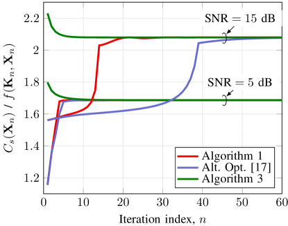
((a)) Joint SPC and PAPC.

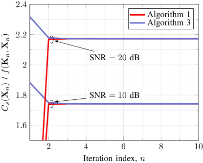
((b)) Joint SPC, PAPC and IPC, .

Figure 1: Convergence results of iterative algorithms for different SNRs and different combination of types of power constraints.

We now demonstrate the usefulness of the convex reformulation of the secrecy capacity problem for the degraded case. Note that in Fig. 1, the convergence rate of the proposed algorithms is shown in terms of iteration counts and the per-iteration complexity is not taken into account. To achieve a more meaningful comparison, we report in Table I the average actual run time of different methods for solving (3) when the MIMO WTC is degraded, i.e. $\mathbf{H}_{b}^{{\dagger}}\mathbf{H}_{b}\succeq\mathbf{H}_{e}^{{\dagger}}\mathbf{H}_{e}$. In this case, the power convex solver MOSEK [33] can be used to solve the convex reformulation and is included for comparison. The average run time in Table I is obtained from 1000 random channel realizations. For Algorithm 1 we use Algorithm 2 to solve the subproblem in each iteration. Similarly, for Algorithm 3 we modify Algorithm 2 to solve (22). The stopping criterion for Algorithms 1 and 3 is when the increase during the last 100 iterations is less than $10^{-5}$. For comparison purpose, we also report the run time of the barrier method presented in [18]. It can be seen that MOSEK is faster to compute the optimal signaling for systems of small sizes. On the other hand, Algorithm 1 becomes more efficient when the size of the system increases.

TABLE I: Comparison of run-time (in seconds) between the proposed method for degraded channels

	$\begin{array}[]{c}(N_{t},N_{r},N_{e})\\ =(4,4,4)\end{array}$		$\begin{array}[]{c}(N_{t},N_{r},N_{e})\\ =(8,8,8)\end{array}$
	5dB	10dB	5dB	10dB
MOSEK	0.25	0.27	2.02	2.01
Algorithm 1	0.9	1.21	1.43	1.79
Algorithm 3	0.88	1.11	1.82	2.81
Minmax barrier method [18]	1.47	1.61	2.58	2.68

In the next numerical experiment we compare the convergence rate of Algorithm 2 with a subgradient method for solving (15). In particular, we plot the convergence of both algorithms for the first subproblem (i.e. $n=1$) in Algorithm 1. The channels are the same as in Fig. 1(a). To make relevant reference to Fig. 1(a), we plot $\underline{C}_{s}(\mathbf{X})$, the lower bound of the secrecy capacity given by

$$\underline{C}_{s}(\mathbf{X})=\bar{f}(\mathbf{X};\mathbf{V}_{0})+\log\bigl{|}\mathbf{I}+\mathbf{H}_{e}\mathbf{V}_{0}\mathbf{H}_{e}^{{\dagger}}\bigr{|}-\operatorname{tr}\bigl{(}\nabla f_{e}(\mathbf{V}_{0})\mathbf{V}_{0}\bigr{)}\leq C_{s}(\mathbf{X})$$

instead of the objective in (15). That is we include the constants omitted when deriving (15). If $\underline{C}_{s}(\mathbf{X})<0$, it is replaced by $0$. We note that Algorithm 2 and the subgradient method are not monotone in general. To make the convergence of these two algorithms easier to visualize, we plot the best $\underline{C}_{s}(\mathbf{X})$ at each iteration. For the subgradient method we use a constant step size rule. It can be seen clearly that Algorithm 2 converges much faster than the subgradient method in the two considered values of SNR. Furthermore, our extensive numerical results show that the convergence rate of Algorithm 2 is less sensitive to the considered settings and it becomes stabilized very quickly. We also observe that the convergence of the subgradient method depends heavily on the choice of the step size. In Fig. 2 we choose a step size such that the subgradient method produces a good convergence performance for the considered setting. However, it cannot guarantee its convergence in many other cases.

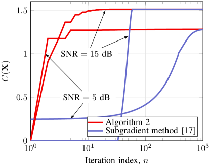
Figure 2: Convergence comparison of Algorithm 2 and the subgradient method [17] for solving (15) for different SNRs.

VI-B Impact of Bob-Eve Correlation

In the next numerical experiment, we investigate the effect of the channel correlation between Bob and Eve on the achieved MIMO secrecy capacity. To this end we fix $\phi_{b}=0$ and vary $\phi_{e}$ and the correlation coefficient $r$ is set to $r=0.9$. We remark that the transmit correlation matrix of Bob’s channel is $\mathbf{R}_{b}=E\{\mathbf{H}_{b}^{{\dagger}}\mathbf{H}_{b}\}$ and of the Eve’s channel is $\mathbf{R}_{e}^{\prime}=E\{\mathbf{H}_{e}^{{\dagger}}\mathbf{H}_{e}\}E\{\mathbf{H}_{e}^{{\dagger}}\mathbf{H}_{e}\}=\gamma^{2}\mathbf{R}_{e}$. The correlation between Bob’s channel and Eve’s channel can be measured by the following quantity [43, Section 3.1.1]

$$d_{\textrm{corr}}=1-\frac{\operatorname{tr}(\mathbf{R}_{b}\mathbf{R}_{e}^{\prime})}{\bigl{\|}\mathbf{R}_{b}\bigr{\|}_{F}\bigl{\|}\mathbf{R}_{e}^{\prime}\bigr{\|}_{F}}=1-\frac{\operatorname{tr}(\mathbf{R}_{b}\mathbf{R}_{e})}{\bigl{\|}\mathbf{R}_{b}\bigr{\|}_{F}\bigl{\|}\mathbf{R}_{e}\bigr{\|}_{F}}$$

Note that the $d_{\textrm{corr}}$ is a function of $\phi_{e}$ and independent of $\gamma$. It is easy to see that if $\mathbf{R}_{b}$ and $\mathbf{R}_{e}$ are identical (apart from a scaling factor), then $d_{\textrm{corr}}=0$. Roughly speaking, a small value of $d_{\textrm{corr}}$ indicates the two links are highly correlated. On the other hand, if $d_{\textrm{corr}}$ is close to 1 means that the two links are highly uncorrelated.

Fig. 3 plots the secrecy capacity as a function of $\phi_{e}$ for two cases of transmit correlation coefficient: $r=0.9$ (highly correlated antennas) and $r=0.2$ (low correlated antennas). For comparison purpose, we also include in Fig. 3 the capacity between Alice and Bob when Eve is not present, and the achieved secrecy rate obtained by the ZF method. Firstly and as expected, the channel capacity in the absence of Eve is always higher than the secrecy capacity. However, for highly correlated antennas in Fig. 3(a), the gap is reduced when $\phi_{e}$ is increased. To explain this, we note that by a direct correlation, can see that $d_{\textrm{corr}}$ increases from $0$ to 0$.96$ when $\phi_{e}$ increases from $0$ to $\pi$. Thus, Bob’s channel and Eve’s channel become more uncorrelated. Intuitively, we can view $\phi_{e}$ increasing from $0$ to $\pi$ as Eve will move further from Bob along a circular arc. As a result, Alice can transmit information securely to Bob through the eigenmodes of $\mathbf{H}_{b}$, without being comprised by the eigenmodes of $\mathbf{H}_{e}$. That is, the information leakage is reduced, which in turn increases the secrecy capacity. Secondly we notice that the secrecy capacity is always higher than the secrecy capacity rate achieved by the ZF precoding method, and the gap is also reduced for the same reason as explained above. We also observe that when the number of antennas at Alice increases from $N_{t}=6$ to $N_{t}=12$, the gap between the secrecy capacity and the secrecy achievable rate obtained by the ZF is very marginal. The reason is that with additional degree of freedom, Alice can now create multiple beams to Bob without being overheard by Eve.

On the other hand, when the transmit antennas are low correlated as considered in Fig. 3(b), the off-diagonal elements of both $\mathbf{R}_{b}$ and $\mathbf{R}_{e}$ are very small, compared to the diagonal elements which are all unity. Thus, both $\mathbf{R}_{b}$ and $\mathbf{R}_{e}$ are very close to the identity matrix and thus $d_{\textrm{corr}}$ is very small for all considered values of $\phi_{e}$. Intuitively, Bob’s link and Eve’s link are highly correlated in this case. As a result, the gap between the channel capacity in the absence of Eve and the secrecy capacity is significant and the position of Eve has little impact on the obtained secrecy capacity.

((a)) $r=0.9$

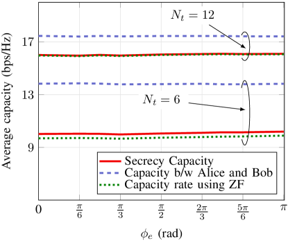
((b)) $r=0.2$

Figure 3: Effect of channel correlation between Bob and Eve on secrecy capacity for $N_{r}=4,N_{e}=3$.

VI-C Impact of Transmit Antenna

We now study how the secrecy capacity scales with the number of transmit antennas at Alice. Fig. 4 plots the average secrecy capacity for various numbers of antennas at Eve for different combinations of power constraints. The number of receiver antennas at Bob is $N_{r}=4$. The correlation coefficient is set to $r=0.9$ and the parameter $\gamma$ is taken $\gamma=0.9$. For Fig. 4(b) we consider the scenario where Alice has to limit the interference to a primary receiver (PR) below a threshold. The channel between Alice and PR is modeled as $\mathbf{H}_{p}=\gamma\tilde{\mathbf{H}}_{p}\mathbf{R}_{p}^{1/2}$, where $\tilde{\mathbf{H}}_{p}$ and $\mathbf{R}_{p}$ are generated in the same way as explained above for Bob’s and Eve’ channels, i.e. $[\mathbf{R}_{p}]_{i,j}=\bigl{(}re^{j\phi_{p}}\bigr{)}{}^{|i-j|}$ where $\phi_{p}=\frac{\pi}{4}$. The number of antennas at the PR is $N_{p}=4$ and the interference threshold at the PR is $5$ dB. As can be seen in Fig. 4, the secrecy capacity increases with the number of the transmit antennas at Alice, which is expected. Simultaneously, we also observe that the secrecy capacity is reduced when the number of antennas at Eve increases. In particular, Eve can significantly decrease the secrecy capacity when $N_{e}$ is much larger than $N_{t}$. This is because the null space of $\mathbf{H}_{b}$ will increasingly intersect with the space spanned by $\mathbf{H}_{e}$. It is also clear from Fig. 4(b) that including the IPC can reduce the secrecy rate.

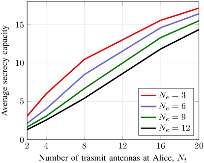
((a)) Power constraints: joint SPC and PAPC

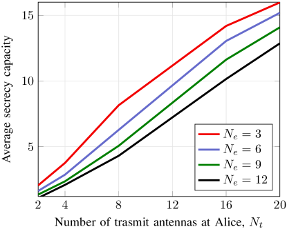
((b)) Power constraints: joint SPC, PAPC and IPC. The number of transmit antennas at the PR is $N_{p}=4$

Figure 4: Secrecy capacity as a function of $N_{t}$ for different values of $N_{e}$ for different combinations of power constraints. The number of receiver antennas at Bob is $N_{r}=4$.

VII Conclusion

We have proposed efficient numerical solutions for finding the secrecy capacity of MIMO WTC subject to joint sum power constraint and per antenna power constraint. This problem is non-convex in general, and thus, is difficult to find an optimal solution. Our first contribution has been a convex reformulation of the secrecy problem for the degraded MIMO WTC. For non-degraded cases, we have proposed ADCA that solves the secrecy problem directly and PBRA that solves the equivalent convex-concave program. In particular, we have also presented the CoMirror algorithm which efficiently solves the subconvex problems resulting from the ADCA and the PBRA. We have carried out numerical experiments to demonstrate the effectiveness of the proposed solutions. In particular, the convergence rate of the proposed algorithm is much faster than a known solution. We have also shown that the transmit antenna correlation at Alice and the number of antennas at Eve have a significant impact on the secrecy capacity. We note that artificial noise is a good technique to enhance physical layer security. In this regard, it is interesting to see if the proposed methods in this paper can be extended to deal with this technology, which deserves a separate through study and thus is left for future work.

-A Proof of Lemma 1

To proceed, we first rewrite $C_{s}(\mathbf{X})$ as

$$C_{s}(\mathbf{X}) =\ln\bigl{|}\mathbf{I}+\mathbf{X}\mathbf{H}_{b}^{{\dagger}}\mathbf{H}_{b}\bigr{|}-\ln\bigl{|}\mathbf{I}+\mathbf{X}\mathbf{H}_{e}^{{\dagger}}\mathbf{H}_{e}\bigr{|}$$

$$=\ln\bigl{|}\mathbf{I}+\mathbf{X}\mathbf{H}_{e}^{{\dagger}}\mathbf{H}_{e}+\mathbf{X}\boldsymbol{\Delta}\bigr{|}-\ln\bigl{|}\mathbf{I}+\mathbf{X}\mathbf{H}_{e}^{{\dagger}}\mathbf{H}_{e}\bigr{|}$$

$$=\ln\bigl{|}\mathbf{I}+\bigl{(}\mathbf{I}+\mathbf{X}\mathbf{H}_{e}^{{\dagger}}\mathbf{H}_{e}\bigr{)}^{-1}\mathbf{X}\boldsymbol{\Delta}\bigr{|}$$

$$=\ln\bigl{|}\mathbf{I}+\boldsymbol{\Delta}^{1/2}\bigl{(}\mathbf{I}+\mathbf{X}\mathbf{H}_{e}^{{\dagger}}\mathbf{H}_{e}\bigr{)}^{-1}\mathbf{X}\boldsymbol{\Delta}^{1/2}\bigr{|}$$ (31)

where we have used the fact that $\ln|\mathbf{I}+\mathbf{A}\mathbf{B}|=\ln|\mathbf{I}+\mathbf{B}\mathbf{A}|$. Using the matrix inversion lemma [44, Fact 2.16.21], we have

$$\bigl{(}\mathbf{I}+\mathbf{X}\mathbf{H}_{e}^{{\dagger}}\mathbf{H}_{e}\bigr{)}^{-1}=\mathbf{I}-\mathbf{X}\mathbf{H}_{e}^{{\dagger}}\bigl{(}\mathbf{I}+\mathbf{H}_{e}\mathbf{X}\mathbf{H}_{e}^{{\dagger}}\bigr{)}^{-1}\mathbf{H}_{e}$$ (32)

and thus $C_{s}(\mathbf{X})$ is further equivalently expressed as

$$C_{s}(\mathbf{X}) =\ln\Bigl{|}\mathbf{I}+\boldsymbol{\Delta}^{1/2}\bigl{(}\mathbf{X}-\mathbf{X}\mathbf{H}_{e}^{{\dagger}}\bigl{(}\mathbf{I}+\mathbf{H}_{e}\mathbf{X}\mathbf{H}_{e}^{{\dagger}}\bigr{)}^{-1}\mathbf{H}_{e}\mathbf{X}\bigr{)}\boldsymbol{\Delta}^{1/2}\Bigr{|}$$

$$=\ln\bigl{|}\mathbf{I}+\boldsymbol{\Delta}^{1/2}\mathbf{X}\boldsymbol{\Delta}^{1/2}-\boldsymbol{\Delta}^{1/2}\mathbf{X}\mathbf{H}_{e}^{{\dagger}}\bigl{(}\mathbf{I}+\mathbf{H}_{e}\mathbf{X}\mathbf{H}_{e}^{{\dagger}}\bigr{)}^{-1}\mathbf{H}_{e}\mathbf{X}\boldsymbol{\Delta}^{1/2}\bigr{|}.$$

The proof is due to some collective results in [32, Section 3.2]. Let $F(\mathbf{X})=\mathbf{I}+\boldsymbol{\Delta}^{1/2}\mathbf{X}\boldsymbol{\Delta}^{1/2}-\boldsymbol{\Delta}^{1/2}\mathbf{X}\mathbf{H}_{e}^{{\dagger}}\bigl{(}\mathbf{I}+\mathbf{H}_{e}\mathbf{X}\mathbf{H}_{e}^{{\dagger}}\bigr{)}^{-1}\mathbf{H}_{e}\mathbf{X}\boldsymbol{\Delta}^{1/2}$ which is a matrix-valued function of $\mathbf{X}$. It is easy to see that (3) is equivalent to

$$\underset{\mathbf{X}\succeq\mathbf{0},\mathbf{Y}\succeq\mathbf{0}}{\mathrm{maximize}} \ \ln|\mathbf{Y}|$$ (33a)

$$\operatorname{subject~{}to} \ F(\mathbf{X})\succeq\mathbf{Y}$$ (33b)

$$\ \mathbf{X}\in\mathcal{X}$$ (33c)

which is in fact a “$\succeq$-epigraph” form of (3). Further note that the constraint $F(\mathbf{X})\succeq\mathbf{Y}$ is equivalent to

$$\mathbf{I}+\boldsymbol{\Delta}^{1/2}\mathbf{X}-\mathbf{Y}-\boldsymbol{\Delta}^{1/2}\mathbf{X}\mathbf{H}_{e}^{{\dagger}}\bigl{(}\mathbf{I}+\mathbf{H}_{e}\mathbf{X}\mathbf{H}_{e}^{{\dagger}}\bigr{)}^{-1}\mathbf{H}_{e}\mathbf{X}\boldsymbol{\Delta}^{1/2}\succeq\mathbf{0}$$

which can be rewritten as (7b) using [32, Lemma 4.2.1] and thus completes the proof.

-B Proof of Lemma 2

We adapt the arguments in [22] for the maximization context. First note that $\mathbf{X}_{n}$ solves (15) and thus we have

$$f_{b}(\mathbf{X}_{n})-\operatorname{tr}\bigl{(}\nabla f_{e}(\mathbf{V}_{n-1})\bigr{)}\mathbf{X}_{n}\geq f_{b}(\mathbf{V}_{n-1})-\operatorname{tr}\bigl{(}\nabla f_{e}(\mathbf{V}_{n-1})\mathbf{V}_{n-1}\bigr{)}$$ (34)

which equivalent to

$$f_{b}(\mathbf{X}_{n})\geq f_{b}(\mathbf{V}_{n-1})-\operatorname{tr}\bigl{(}\nabla f_{e}(\mathbf{V}_{n-1})\bigl{(}\mathbf{V}_{n-1}-\mathbf{X}_{n}\bigr{)}\bigr{)}$$ (35)

The concavity of $f_{e}(\mathbf{X})$ implies

$$f_{e}(\mathbf{X}_{n})\leq f_{e}(\mathbf{V}_{n-1})+\operatorname{tr}\left(\nabla f_{b}(\mathbf{V}_{n-1})\bigl{(}\mathbf{X}_{n}-\mathbf{V}_{n-1}\bigr{)}\right)$$ (36)

Combining (35) and (36) yields

$$C_{s}(\mathbf{X}_{n})=f_{b}(\mathbf{X}_{n})-f_{e}(\mathbf{X}_{n})\geq f_{b}(\mathbf{V}_{n-1})-f_{e}(\mathbf{V}_{n-1})=C_{s}(\mathbf{V}_{n-1}).$$ (37)

It follows from Step 7 of Algorithm 1 that

$$C(\mathbf{V}_{n-1})\geq\min\bigl{(}C_{s}(\mathbf{X}_{n-1}),C_{s}(\mathbf{X}_{n-2}),\ldots,C(\mathbf{X}_{[n-1-q]_{+}})\bigr{)}=\gamma_{n-1}.$$ (38)

and thus we obtain

$$C_{s}(\mathbf{X}_{n})\geq C_{s}(\mathbf{V}_{n-1})\geq\gamma_{n-1}.$$ (39)

Consequently the following inequality also holds

$$C_{s}(\mathbf{X}_{n+1}) \geq\gamma_{n}=\min\bigl{(}C_{s}(\mathbf{X}_{n}),C_{s}(\mathbf{X}_{n-1}),\ldots,C(\mathbf{X}_{[n-q]_{+}})\bigr{)}$$ (40a)

$$\geq\min\bigl{(}C_{s}(\mathbf{X}_{n}),C_{s}(\mathbf{X}_{n-1}),\ldots,C(\mathbf{X}_{n+1-q}),C(\mathbf{X}_{[n-q]_{+}}),C(\mathbf{X}_{[n-1-q]_{+}})\bigr{)}$$ (40b)

$$\geq\min\bigl{(}C_{s}(\mathbf{X}_{n}),\gamma_{n-1}\bigr{)}=\gamma_{n-1}.$$ (40c)

By repeating this process we can easily see that

$$C_{s}(\mathbf{X}_{n+m})\geq\gamma_{n-1},m=0,1,\ldots,q.$$ (41)

Therefore we obtain

$$\gamma_{n+q} =\min\bigl{(}C_{s}(\mathbf{X}_{n+q}),C_{s}(\mathbf{X}_{n+q-1}),\ldots,C(\mathbf{X}_{n})\bigr{)}$$ (42a)

$$\geq\min\bigl{(}C_{s}(\mathbf{X}_{n+q}),\gamma_{n-1}\bigr{)}=\gamma_{n-1}$$ (42b)

where (42b) follows from (41).

It is easy to check that the sequence $\{\gamma_{n}\}$ is bounded above and thus is convergent. Also, since the feasible set $\mathcal{X}$ is compact and convex, there exist a convergent subsequence. Let $\mathbf{X}_{n_{j}}$ be the subsequence converging to a limit point $\mathbf{X}^{\ast}$. Without loss of generality, we assume that $\mathbf{V}_{n_{j}-1}$ converges to a limit point $\mathbf{V}^{\ast}$. Due to the strict concavity and continuity of the objective in each subproblem, it must follow that $\mathbf{X}^{\ast}=\mathbf{V}^{\ast}$. Since $\mathbf{X}_{n_{j}}$ is the solution to (15) we have

$$\operatorname{tr}\bigl{(}\nabla f_{b}(\mathbf{X}_{n_{j}})-\nabla f_{e}(\mathbf{V}_{n_{j}-1})\bigr{)}\bigl{(}\mathbf{X}-\mathbf{X}_{n_{j}}\bigr{)}\leq 0,\forall\mathbf{X}\in\mathcal{X}.$$ (43)

Let $j\to\infty$ give $\operatorname{tr}\bigl{(}\nabla f_{b}(\mathbf{X}^{\ast})-\nabla f_{e}(\mathbf{X}^{\ast})\bigr{)}\bigl{(}\mathbf{X}-\mathbf{X}^{\ast}\bigr{)}\leq 0,\forall\mathbf{X}\in\mathcal{X}$, meaning that $\mathbf{X}^{\ast}$ is a critical point of (3) and thus completes the proof.

-C Convergence Analysis of Algorithm 2

Algorithm 2 is a special case of the CoMirror Algorithm in [23] when the distance generating function (also known as the kernel function of the mirror map) [45] is chosen as $\Theta(\mathbf{X})=\frac{1}{2}\left\|\mathbf{X}\right\|_{F}^{2}$ and the associated norm over $\mathcal{X}_{\mathrm{spc}}$ is the Frobenius norm. For a given initial point $\mathbf{X}^{0}\in\mathcal{X}_{\textrm{spc}}$, the parameter $\Omega$ is defined as

$$\Omega=\frac{1}{\sqrt{2}}\underset{\mathbf{X}\in\mathcal{X}_{\textrm{spc}}}{\max}\ \bigl{\|}\mathbf{X}-\mathbf{X}^{0}\bigr{\|}_{F}.$$

If $\mathbf{X}^{0}=\mathbf{0}$, then it is easy to see that $\Omega\leq\frac{1}{\sqrt{2}}P_{0}$. In general we can find of an upper bound of $\Omega$ as

$$\Omega =\frac{1}{\sqrt{2}}\underset{\mathbf{X}\in\mathcal{X}_{\textrm{spc}}}{\max}\ \bigl{\|}\mathbf{X}-\mathbf{X}^{0}\bigr{\|}_{F}=\frac{1}{\sqrt{2}}\underset{\mathbf{X}\in\mathcal{X}_{\textrm{spc}}}{\max}\ \bigl{\|}\mathbf{X}-\mathbf{X}^{0}\bigr{\|}_{F}$$

$$=\frac{1}{\sqrt{2}}\underset{\mathbf{X}\in\mathcal{X}_{\textrm{spc}}}{\max}\sqrt{\bigl{\|}\mathbf{X}\bigr{\|}_{F}^{2}-2\operatorname{tr}\bigl{(}\mathbf{X}^{0}\mathbf{X}\bigr{)}+\bigl{\|}\mathbf{X}^{0}\bigr{\|}_{F}^{2}}$$

$$\leq\sqrt{\frac{P_{0}^{2}+\bigl{\|}\mathbf{X}^{0}\bigr{\|}_{F}^{2}}{2}}.$$

The next step is show that $\nabla g_{m}(\mathbf{X})=\operatorname{diag}(\mathbf{e}_{m})$, where $m=\underset{1\leq i\leq N_{t}}{\arg\max}g_{i}(\mathbf{X})$ is a subgradient of the pointwise maximum $g(\mathbf{X})=\underset{1\leq i\leq N_{t}}{\max}g_{i}(\mathbf{X})$. This is a trivial result since $g_{m}(\mathbf{X})$ is an active function at $\mathbf{X}$ (i.e. $g(\mathbf{X})=g_{m}(\mathbf{X})$). It is also easy to see that $\bigl{\|}\nabla g_{m}(\mathbf{X})\bigr{\|}_{F}\leq 1$ and thus is bounded. The final step to establish the convergence of Algorithm 2 is to show that $\bigl{\|}\nabla\bar{f}(\mathbf{X})\bigr{\|}_{F}$ is bounded. To this end, we recall that

$$\nabla_{\mathbf{X}}\bar{f}(\mathbf{X})=\mathbf{H}_{b}^{{\dagger}}(\mathbf{I}+\mathbf{H}_{b}\mathbf{X}\mathbf{H}_{b}^{{\dagger}})^{-1}\mathbf{H}_{b}-\boldsymbol{\Gamma}_{n-1}$$ (44)

and thus

$$\left\|\nabla_{\mathbf{X}}\bar{f}(\mathbf{X})\right\|_{F} \leq\left\|\boldsymbol{\Gamma}_{n-1}\right\|_{F}+\bigl{\|}\mathbf{H}_{b}^{{\dagger}}(\mathbf{I}+\mathbf{H}_{b}\mathbf{X}\mathbf{H}_{b}^{{\dagger}})^{-1}\mathbf{H}_{b}\bigr{\|}_{F}$$

$$\leq\left\|\boldsymbol{\Gamma}_{n-1}\right\|_{F}+\bigl{\|}\mathbf{H}_{b}^{{\dagger}}\mathbf{H}_{b}\bigr{\|}_{F}$$ (45)

which holds because $(\mathbf{I}+\mathbf{H}_{b}\mathbf{X}\mathbf{H}_{b}^{{\dagger}})^{-1}\preceq\mathbf{I}$ for $\mathbf{X}\succeq\mathbf{0}$.

-D Proof of Lemma 4

A very brief proof of Lemma 4 was provided in [14]. Herein we present a more rigorous proof. The idea is based on manipulating the Karush-Kuhn-Tucker (KKT) conditions of problem 29. Since problem (29a) is convex and strong duality holds, KKT conditions are necessary and sufficient for an optimal solution. Let $\mathbf{Z}$ be the Lagrangian multiplier for the constraint $\mathbf{I}-\bar{\mathbf{K}}\bar{\mathbf{K}}^{{\dagger}}\succeq\mathbf{0}$. Then the KKT conditions of (29a) are given by

$$\boldsymbol{\Psi}_{12}+(\mathbf{I}-\bar{\mathbf{K}}\bar{\mathbf{K}}^{{\dagger}})^{-1}\bar{\mathbf{K}}+\mathbf{Z}\bar{\mathbf{K}} =0$$ (46a)

$$\mathbf{I}-\bar{\mathbf{K}}\bar{\mathbf{K}}^{{\dagger}} \succeq\mathbf{0}$$ (46b)

$$\mathbf{Z} \succeq\mathbf{0}$$ (46c)

$$\operatorname{tr}\left(\left(\mathbf{I}-\bar{\mathbf{K}}\bar{\mathbf{K}}^{{\dagger}}\right)\mathbf{Z}\right) =\mathbf{0}$$ (46d)

where we have used the results in [24] to obtain (46a). Let us assume for the moment that $\mathbf{I}-\bar{\mathbf{K}}\bar{\mathbf{K}}^{{\dagger}}\succ\mathbf{0}$. Then it follows immediately from (46d) that $\mathbf{Z}=\mathbf{0}$ and thus we have

$$(\mathbf{I}-\bar{\mathbf{K}}\bar{\mathbf{K}}^{{\dagger}})^{-1}\bar{\mathbf{K}}=-\boldsymbol{\Psi}_{12}$$ (47)

which yields

$$(\mathbf{I}-\bar{\mathbf{K}}\bar{\mathbf{K}}^{{\dagger}})^{-1}\bar{\mathbf{K}}\bar{\mathbf{K}}^{{\dagger}}(\mathbf{I}-\bar{\mathbf{K}}\bar{\mathbf{K}}^{{\dagger}})^{-1}=\boldsymbol{\Psi}_{12}\boldsymbol{\Psi}_{12}^{{\dagger}}.$$ (48)

Let $\bar{\mathbf{K}}\bar{\mathbf{K}}^{{\dagger}}=\mathbf{U}_{\bar{\mathbf{K}}}\bar{\boldsymbol{\Sigma}}_{\bar{\mathbf{K}}}\mathbf{U}_{\bar{\mathbf{K}}}^{\dagger}$ and $\boldsymbol{\Psi}_{12}\boldsymbol{\Psi}_{12}^{{\dagger}}=\mathbf{U}_{\mathbf{\boldsymbol{\Psi}}}\bar{\boldsymbol{\Sigma}}_{\mathbf{\mathbf{\boldsymbol{\Psi}}}}\mathbf{U}_{\mathbf{\boldsymbol{\Psi}}}^{\dagger}$ be the eigenvalue decomposition of $\mathbf{\bar{\mathbf{K}}\bar{\mathbf{K}}^{{\dagger}}}$ and $\boldsymbol{\Psi}\boldsymbol{\Psi}^{{\dagger}}$, respectively, where $\mathbf{U}_{\bar{\mathbf{K}}}\in\mathbb{C}^{N_{r}\times N_{r}}$ and $\mathbf{U}_{\boldsymbol{\Psi}}\in\mathbb{C}^{N_{r}\times N_{r}}$ are unitary and $\bar{\boldsymbol{\Sigma}}_{\bar{\mathbf{K}}}=\operatorname{diag}(\sigma_{\bar{\mathbf{K}}_{1}},\sigma_{\bar{\mathbf{K}}_{2}},\ldots,\sigma_{\bar{\mathbf{K}}_{N_{r}}})$ $\bar{\boldsymbol{\Sigma}}_{\mathbf{\mathbf{\boldsymbol{\Psi}}}}=\operatorname{diag}(\sigma_{\boldsymbol{\Psi}_{1}},\sigma_{\boldsymbol{\Psi}_{2}},\ldots,\sigma_{\boldsymbol{\Psi}_{N_{r}}})$. Note that $\sigma_{\bar{\mathbf{K}}_{i}}$and $\sigma_{\boldsymbol{\Psi}_{i}}$ are the eigenvalues of $\bar{\mathbf{K}}\bar{\mathbf{K}}^{{\dagger}}$ and $\boldsymbol{\Psi}\boldsymbol{\Psi}^{{\dagger}}$, respectively. Then (48) is equivalent to

$$\mathbf{U}_{\bar{\mathbf{K}}}(\mathbf{I}-\bar{\boldsymbol{\Sigma}}_{\bar{\mathbf{K}}})^{-1}\bar{\boldsymbol{\Sigma}}_{\bar{\mathbf{K}}}(\mathbf{I}-\bar{\boldsymbol{\Sigma}}_{\bar{\mathbf{K}}})^{-1}\mathbf{U}_{\bar{\mathbf{K}}}^{\dagger}=\mathbf{U}_{\boldsymbol{\Psi}}\bar{\boldsymbol{\Sigma}}_{\boldsymbol{\Psi}}\mathbf{U}_{\boldsymbol{\Psi}}^{\dagger}.$$ (49)

Thus we can set

$$\mathbf{U}_{\bar{\mathbf{K}}} =\mathbf{U}_{\boldsymbol{\Psi}}$$ (50a)

$$(\mathbf{I}-\bar{\boldsymbol{\Sigma}}_{\bar{\mathbf{K}}})^{-1}\bar{\boldsymbol{\Sigma}}_{\bar{\mathbf{K}}}(\mathbf{I}-\bar{\boldsymbol{\Sigma}}_{\bar{\mathbf{K}}})^{-1} =\bar{\boldsymbol{\Sigma}}_{\boldsymbol{\Psi}}$$ (50b)

and the objective is to find $\bar{\boldsymbol{\Sigma}}_{\bar{\mathbf{K}}}$ such that (50b) is satisfied. It is easy to see that (49) gives

$$\frac{\sigma_{\bar{\mathbf{K}}_{i}}}{(1-\sigma_{\bar{\mathbf{K}}_{i}})^{2}}=\sigma_{\boldsymbol{\Psi}_{i}},i=1,2,\ldots,N_{r}$$ (51)

Solving for $\sigma_{\bar{\mathbf{K}}_{i}}$yields

$$\sigma_{\bar{\mathbf{K}}_{i}}=\begin{cases}0&\sigma_{\Psi_{i}}=0\\ 0.5\left\{\left(2+\frac{1}{\sigma_{\boldsymbol{\Psi}_{i}}}\right)-\sqrt{\left(2+\frac{1}{\sigma_{\boldsymbol{\Psi}_{i}}}\right)^{2}-4}\right\}&\sigma_{\Psi_{i}}>0.\end{cases}$$ (52)

We remark that $1>\sigma_{\bar{\mathbf{K}}_{i}}$, $\forall i=1,2,\ldots,N_{r}$ and thus $\mathbf{I}-\bar{\mathbf{K}}\bar{\mathbf{K}}^{{\dagger}}\succ\mathbf{0}$ as assumed above and it satisfies the KKT conditions. After some algebraic steps we simplify the above equation as

$$\sigma_{\bar{\mathbf{K}}_{i}}=\frac{4\sigma_{\boldsymbol{\Psi}_{i}}}{\bigl{(}1+\sqrt{1+4\sigma_{\boldsymbol{\Psi}_{i}}}\bigr{)}^{2}}$$ (53)

and thus

$$\mathbf{I}-\bar{\mathbf{K}}\bar{\mathbf{K}}^{{\dagger}}=2\mathbf{U}_{\bar{\mathbf{K}}}\operatorname{diag}\biggl{(}\frac{1}{1+\sqrt{1+4\sigma_{\boldsymbol{\Psi}_{1}}}},\frac{1}{1+\sqrt{1+4\sigma_{\boldsymbol{\Psi}_{2}}}},\ldots,\frac{1}{1+\sqrt{1+4\sigma_{\boldsymbol{\Psi}_{N_{r}}}}}\biggr{)}\mathbf{U}_{\bar{\mathbf{K}}}^{{\dagger}}.$$

Multiplying both sides of (47) with $\mathbf{I}-\bar{\mathbf{K}}\bar{\mathbf{K}}^{{\dagger}}$ and using the above equation results in which completes the proof.

-E Proof of Lemma 5

First we note that for a given $\mathbf{K}_{n}$, $\mathbf{X}_{n}$ is the capacity achieving covariance matrix of the combined MIMO channel that contains both $\mathbf{H}_{b}$ and $\mathbf{H}_{e}$ where $\mathbf{K}_{n}$ is the effective noise [8]. Thus, $f(\mathbf{X}_{n},\mathbf{K}_{n})$ is always non-negative $f(\mathbf{X}_{n},\mathbf{K}_{n})\geq 0$. The main idea behind the proof of the monotonic decrease of the objective sequence $\{f(\mathbf{K}_{n},\mathbf{X}_{n})\}$ is to exploit the fact that the term $\log|\mathbf{K}+\mathbf{H}\mathbf{X}\mathbf{H}^{{\dagger}}|-\log|\mathbf{I}+\mathbf{H}_{e}\mathbf{X}\mathbf{H}_{e}^{{\dagger}}|$ is jointly concave with $\mathbf{K}$ and $\mathbf{X}$. In this regard, the following inequality is straightforward

$$f(\mathbf{K},\mathbf{X}) \leq\log|\mathbf{K}_{n}+\mathbf{H}\mathbf{X}_{n}\mathbf{H}^{{\dagger}}|+\operatorname{tr}(\boldsymbol{\Psi}_{n}(\mathbf{K}-\mathbf{K}_{n}))$$

$$\quad+\operatorname{tr}(\boldsymbol{\Phi}_{n}(\mathbf{X}-\mathbf{X}_{n}))-\log|\mathbf{K}|-\log|\mathbf{I}+\mathbf{H}_{e}\mathbf{X}_{n}\mathbf{H}_{e}^{{\dagger}}|,\forall\mathbf{K}\in\mathcal{K}.$$ (54)

where $\boldsymbol{\Phi}_{n}=\mathbf{H}^{{\dagger}}\bigl{(}\mathbf{K}_{n}+\mathbf{H}\mathbf{X}_{n}\mathbf{H}^{{\dagger}}\bigr{)}^{-1}\mathbf{H}-\mathbf{H}_{e}^{{\dagger}}\bigl{(}\mathbf{I}+\mathbf{H}_{e}\mathbf{X}_{n}\mathbf{H}_{e}^{{\dagger}}\bigr{)}^{-1}\mathbf{H}_{e}$. The above inequality is nothing but an affine approximation of $\log|\mathbf{K}+\mathbf{H}\mathbf{X}\mathbf{H}^{{\dagger}}|-\log|\mathbf{I}+\mathbf{H}_{e}\mathbf{X}\mathbf{H}_{e}^{{\dagger}}$ around the point $(\mathbf{X}_{n},\mathbf{K}_{n})$. Substituting $(\mathbf{K},\mathbf{X}):=(\mathbf{K}_{n+1},\mathbf{X}_{n+1})$ into (54) we obtain

$$f(\mathbf{K}_{n+1},\mathbf{X}_{n+1}) \leq\log|\mathbf{K}_{n}+\mathbf{H}\mathbf{X}_{n}\mathbf{H}^{{\dagger}}|-\log\bigl{(}\mathbf{K}_{n+1}\bigr{)}$$

$$-\log|\mathbf{I}+\mathbf{H}_{e}\mathbf{X}_{n}\mathbf{H}_{e}^{{\dagger}}|+\operatorname{tr}(\boldsymbol{\Psi}_{n}(\mathbf{K}_{n+1}-\mathbf{K}_{n}))+\operatorname{tr}(\boldsymbol{\Phi}_{n}(\mathbf{X}_{n+1}-\mathbf{X}_{n}))$$

Since $\mathbf{X}_{n}$ is the solution to (22) the first order optimality condition implies

$$\operatorname{tr}\bigl{(}\boldsymbol{\Phi}_{n}\bigl{(}\mathbf{X}-\mathbf{X}_{n}\bigr{)}\bigr{)}\leq 0,\forall\mathbf{X}\in\mathcal{X}.$$ (55)

Substituting $\mathbf{X}$ by $\mathbf{X}_{n+1}$ yields

$$\operatorname{tr}\Bigl{(}\boldsymbol{\Phi}_{n}\bigl{(}\mathbf{X}_{n+1}-\mathbf{X}_{n}\bigr{)}\leq 0,$$ (56)

and thus

$$f(\mathbf{K}_{n+1},\mathbf{X}_{n+1})\leq\log|\mathbf{K}_{n}+\mathbf{H}\mathbf{X}_{n}\mathbf{H}^{{\dagger}}|-\log|\mathbf{K}_{n+1}|\\ -\log|\mathbf{I}+\mathbf{H}_{e}\mathbf{X}_{n}\mathbf{H}_{e}^{{\dagger}}|+\operatorname{tr}(\boldsymbol{\Psi}_{n}(\mathbf{K}_{n+1}-\mathbf{K}_{n})).$$ (57)

Next we will turn our attention to the $\mathbf{K}$ update. Since $\mathbf{K}_{n+1}$ solves (25), we have

$$\operatorname{tr}(\boldsymbol{\Psi}_{n}\mathbf{K}_{n+1})-\log|\mathbf{K}_{n+1}|\leq\operatorname{tr}(\boldsymbol{\Psi}_{n}\mathbf{K})-\log|\mathbf{K}|,\forall\mathbf{K}\in\mathcal{K}$$ (58)

which is true due to the fact that the optimal objective is less than or equal to the objective of any feasible solution. Substituting $\mathbf{K}:=\mathbf{K}_{n}$ into the above inequality gives

$$\operatorname{tr}\bigl{(}\boldsymbol{\Psi}_{n}\mathbf{K}_{n+1}\bigr{)}-\log\bigl{|}\mathbf{K}_{n+1}\bigr{|}\leq\operatorname{tr}(\boldsymbol{\Psi}_{n}\mathbf{K}_{n})-\log\bigl{|}\mathbf{K}_{n}\bigr{|},\forall\mathbf{K}\in\mathcal{K}$$ (59)

which is equivalent to

$$\operatorname{tr}\bigl{(}\boldsymbol{\Psi}_{n}\bigl{(}\mathbf{K}_{n+1}-\mathbf{K}_{n}\bigr{)}\bigr{)}-\log\bigl{|}\mathbf{K}_{n+1}\bigr{|}\leq-\log\bigl{|}\mathbf{K}_{n}\bigr{|}$$ (60)

We note that the above inequality is strict if $\mathbf{K}_{n+1}\neq\mathbf{K}_{n}$. Combining (57) and (60) we obtain

$$f(\mathbf{K}_{n+1},\mathbf{X}_{n+1}) \leq\log|\mathbf{K}_{n}+\mathbf{H}\mathbf{X}_{n}\mathbf{H}^{{\dagger}}|-\log\bigl{|}\mathbf{K}_{n}\bigr{|}-\log|\mathbf{I}+\mathbf{H}_{e}\mathbf{X}_{n}\mathbf{H}_{e}^{{\dagger}}|=f(\mathbf{K}_{n},\mathbf{X}_{n}).$$

References

- [1] A. Mukherjee, B. Ottersten, and L. Tran, “Efficient numerical methods for secrecy capacity of Gaussian MIMO wiretap channel,” in Proc. IEEE VTC 2021, May 2021. [Online]. Available: https://arxiv.org/abs/2102.10396
- [2] C. E. Shannon, “Communication theory of secrecy systems,” The Bell System Technical Journal, vol. 28, no. 4, pp. 656–715, Oct. 1949.
- [3] A. D. Wyner, “The wire-tap channel,” Bell System Technical Journal, vol. 54, no. 8, pp. 1355–1387, 1975.
- [4] S. Leung-Yan-Cheong and M. Hellman, “The Gaussian wire-tap channel,” IEEE Trans. Inf. Theory, vol. 24, no. 4, pp. 451–456, 1978.
- [5] Z. Li, W. Trappe, and R. Yates, “Secret communication via multi-antenna transmission,” in 41st Annual Conference on Information Sciences and Systems 2007, Mar. 2007, pp. 905–910.
- [6] A. Khisti and G. W. Wornell, “Secure transmission with multiple antennas I: The MISOME wiretap channel,” IEEE Trans. Inf. Theory, vol. 56, no. 7, pp. 3088–3104, Jun. 2010.
- [7] ——, “Secure transmission with multiple antennas part II: The MIMOME wiretap channel,” IEEE Trans. Inf. Theory, vol. 56, no. 11, pp. 5515–5532, Oct. 2010.
- [8] F. Oggier and B. Hassibi, “The secrecy capacity of the MIMO wiretap channel,” IEEE Trans. Inf. Theory, vol. 57, no. 8, pp. 4961–4972, Aug 2011.
- [9] J. Li and A. Petropulu, “Optimal input covariance for achieving secrecy capacity in Gaussian MIMO wiretap channels,” in Proc. IEEE ICASSP 2010, Mar. 2010, pp. 3362–3365.
- [10] S. Fakoorian and A. L. Swindlehurst, “Full rank solutions for the MIMO Gaussian wiretap channel with an average power constraint,” IEEE Trans. Signal Process., vol. 61, no. 10, pp. 2620–2631, Mar. 2013.
- [11] S. Loyka and C. D. Charalambous, “Optimal signaling for secure communications over Gaussian MIMO wiretap channels,” in IEEE Trans. Inf. Theory, vol. 62, no. 12, Dec. 2016, pp. 7207–7215.
- [12] J. Steinwandt, S. A. Vorobyov, and M. Haardt, “Secrecy rate maximization for MIMO Gaussian wiretap channels with multiple eavesdroppers via alternating matrix POTDC,” in Proc. IEEE ICASSP 2014, May 2014, pp. 5686–5690.
- [13] K. Cumanan, Z. Ding, B. Sharif, G. Y. Tian, and K. K. Leung, “Secrecy rate optimizations for a MIMO secrecy channel with a multiple-antenna eavesdropper,” IEEE Trans. Veh. Technol., vol. 63, no. 4, pp. 1678–1690, May 2014.
- [14] T. V. Nguyen, Q.-D. Vu, M. Juntti, and L.-N. Tran, “A Low-Complexity Algorithm for Achieving Secrecy Capacity in MIMO Wiretap Channels,” in Proc. IEEE ICC 2020, Jun. 2020.
- [15] T. M. Pham, R. Farrell, H. Claussen, M. Flanagan, and L. Tran, “On the MIMO capacity with multiple linear transmit covariance constraints,” in Proc. IEEE 87th VTC Spring 2018, Jun. 2018, pp. 1–6.
- [16] T. M. Pham, R. Farrell, and L. Tran, “Revisiting the MIMO capacity with per-antenna power constraint: Fixed-point iteration and alternating optimization,” IEEE Trans. Commun., vol. 18, no. 1, pp. 388–401, Jan. 2019.
- [17] Q. Li, M. Hong, H. Wai, W. Ma, Y. Liu, and Z. Luo, “An alternating optimization algorithm for the MIMO secrecy capacity problem under sum power and per-antenna power constraints,” in Proc. IEEE ICASSP 2013, May 2013, pp. 4359–4363.
- [18] S. Loyka and C. D. Charalambous, “An algorithm for global maximization of secrecy rates in Gaussian MIMO wiretap channels,” IEEE Trans. Commun., vol. 63, no. 6, pp. 2288–2299, Jun. 2015.
- [19] P. L. Cao and T. J. Oechtering, “Optimal transmit strategies for Gaussian MISO wiretap channels,” IEEE Trans. Inf. Forensics Secur., vol. 15, pp. 829–838, 2020.
- [20] L. Dong, S. Loyka, and Y. Li, “The secrecy capacity of Gaussian MIMO wiretap channels under interference constraints,” IEEE J. Sel. Areas Commun., vol. 36, no. 4, pp. 704–722, Apr. 2018.
- [21] S. Loyka and L. Dong, “Optimal full-rank signaling over MIMO wiretap channels under interference constraint,” IEEE Wirel. Commun. Lett., vol. 7, no. 4, pp. 534–537, Aug. 2018.
- [22] D. N. Phan, H. M. Le, and H. A. Le Thi, “Accelerated difference of convex functions algorithm and its application to sparse binary logistic regression,” in Proc. Twenty-Seventh Int. Jt. Conf. Artif. Intell., Jul. 2018, pp. 1369–1375.
- [23] A. Beck, A. Ben-Tal, N. Guttmann-Beck, and L. Tetruashvili, “The CoMirror algorithm for solving nonsmooth constrained convex problems,” Oper. Res. Lett., vol. 38, no. 6, pp. 493–498, Nov. 2010.
- [24] A. Hjorungnes and D. Gesbert, “Complex-valued matrix differentiation: Techniques and key results,” IEEE Trans. Signal Process., vol. 55, no. 6, pp. 2740–2746, June 2007.
- [25] Q. Li, M. Hong, H.-T. Wai, Y.-F. Liu, W.-K. Ma, and Z.-Q. Luo, “Transmit solutions for MIMO wiretap channels using alternating optimization,” IEEE J. Sel. Areas Commun., vol. 31, no. 9, pp. 1714–1727, Sep. 2013.
- [26] J. Li and A. Petropulu, “Transmitter optimization for achieving secrecy capacity in Gaussian MIMO wiretap channels,” sep 2009. [Online]. Available: http://arxiv.org/abs/0909.2622
- [27] A. Khina, Y. Kochman, and A. Khisti, “The MIMO wiretap channel decomposed,” vol. 64, no. 2, pp. 1046–1063, Jun. 2018.
- [28] S. Bashar, Z. Ding, and C. Xiao, “On secrecy rate analysis of MIMO wiretap channels driven by finite-alphabet input,” IEEE Trans. Commun., vol. 60, no. 12, pp. 3816–3825, 2012.
- [29] Q. Shi, W. Xu, J. Wu, E. Song, and Y. Wang, “Secure beamforming for MIMO broadcasting with wireless information and power transfer,” IEEE Trans. Wireless Commun., vol. 14, no. 5, pp. 2841–2853, May 2015.
- [30] M. Grant and S. Boyd, “CVX: Matlab software for disciplined convex programming, version 2.2,” http://cvxr.com/cvx, Jan. 2020.
- [31] J. Lofberg, “YALMIP : a toolbox for modeling and optimization in MATLAB,” in Proc. IEEE International Conference on Robotics and Automation 2004, 2004, pp. 284–289.
- [32] A. Ben-Tal and A. Nemirovski, Lectures on Modern Convex Optimization. Society for Industrial and Applied Mathematics, 2001.
- [33] M. ApS, The MOSEK optimization toolbox for MATLAB manual. Version 9.2, 2020. [Online]. Available: https://docs.mosek.com/9.2/toolbox/index.html
- [34] R. Bustin, R. Liu, H. Vincent Poor, and S. Shamai, “An MMSE approach to the secrecy capacity of the MIMO Gaussian wiretap channel,” EURASIP J. Wirel. Commun. Netw., vol. 370970, Jul. 2009.
- [35] J. Steinwandt, S. A. Vorobyov, and M. Haardt, “Secrecy rate maximization for MIMO Gaussian wiretap channels with multiple eavesdroppers via alternating matrix POTDC,” in Proc. IEEE ICASSP 2014, May 2014, pp. 5686–5690.
- [36] Q. H. Spencer, A. L. Swindlehurst, and M. Haardt, “Zero-forcing methods for downlink spatial multiplexing in multiuser MIMO channels,” IEEE Trans. Signal Process., vol. 52, no. 2, pp. 461–471, Feb. 2004.
- [37] S. Boyd and L. Vandenberghe, Convex Optimization. Cambridge University Press, 2004.
- [38] L. Condat, “Fast projection onto the simplex and the ball,” Math. Program., vol. 158, no. 1-2, pp. 575–585, Jul. 2016.
- [39] L. Dong, S. Loyka, and Y. Li, “Algorithms for globally-optimal secure signaling over gaussian MIMO wiretap channels under interference constraints,” IEEE Trans. Signal Process., vol. 68, pp. 4513–4528, Jul. 2020.
- [40] Chen-Nee Chuah, D. N. C. Tse, J. M. Kahn, and R. A. Valenzuela, “Capacity scaling in MIMO wireless systems under correlated fading,” IEEE Trans. Inf. Theory, vol. 48, no. 3, pp. 637–650, Mar. 2002.
- [41] J. P. Kermoal, L. Schumacher, K. I. Pedersen, P. E. Mogensen, and F. Frederiksen, “A stochastic MIMO radio channel model with experimental validation,” IEEE J. Sel. Areas Commun., vol. 20, no. 6, pp. 1211–1226, Aug. 2002.
- [42] S. L. Loyka, “Channel capacity of MIMO architecture using the exponential correlation matrix,” IEEE Commun. Lett., vol. 5, no. 9, pp. 369–371, Sep. 2001.
- [43] B. Clerckx and Claude Oestges, MIMO Wireless Networks. Elsevier, 2013.
- [44] D. S. Bernstein, Matrix Mathematics: Theory, Facts, and Formulas (Second Edition). Princeton University Press, 2009.
- [45] A. Juditsky and A. Nemirovski, “First-Order Methods for Nonsmooth Convex Large-Scale Optimization, I: General Purpose Methods,” in Optim. Mach. Learn. The MIT Press, 2011.