Learning Graphons via Structured Gromov-Wasserstein Barycenters

Abstract

We propose a novel and principled method to learn a nonparametric graph model called graphon, which is defined in an infinite-dimensional space and represents arbitrary-size graphs. Based on the weak regularity lemma from the theory of graphons, we leverage a step function to approximate a graphon. We show that the cut distance of graphons can be relaxed to the Gromov-Wasserstein distance of their step functions. Accordingly, given a set of graphs generated by an underlying graphon, we learn the corresponding step function as the Gromov-Wasserstein barycenter of the given graphs. Furthermore, we develop several enhancements and extensions of the basic algorithm, $e.g.$, the smoothed Gromov-Wasserstein barycenter for guaranteeing the continuity of the learned graphons and the mixed Gromov-Wasserstein barycenters for learning multiple structured graphons. The proposed approach overcomes drawbacks of prior state-of-the-art methods, and outperforms them on both synthetic and real-world data. The code is available at https://github.com/HongtengXu/SGWB-Graphon.

Introduction

Given a set of graphs, $e.g.$, social networks and biological networks, we are often interested in modeling their generative mechanisms and building statistical graph models (Kolaczyk 2009; Goldenberg et al. 2010). Many efforts have been made to achieve this aim, leading to such methods as the stochastic block model (Nowicki and Snijders 2001), the graphlet (Soufiani and Airoldi 2012), and the latent space model (Hoff, Raftery, and Handcock 2002). However, when dealing with large-scale complex networks, the parametric models above are often oversimplified, and thus, suffer from underfitting. To enhance the model capacity, a nonparametric graph model called graphon (or graph limit) was proposed (Janson and Diaconis 2008; Lovász 2012). Mathematically, a graphon is a two-dimensional symmetric Lebesgue measurable function, denoted as $W:\Omega^{2}\mapsto[0,1]$, where $\Omega$ is a measure space, $e.g.$, $\Omega=[0,1]$. Given a graphon, we can generate arbitrarily sized graphs by the following sampling process:

$$\begin{aligned} &v_{n}&&\sim\text{Uniform}(\Omega),~{}\text{for}~{}n=1,...,N,\\ &a_{nn^{\prime}}&&\sim\text{Bernoulli}(W(v_{n},v_{n^{\prime}})),~{}\text{for}~{}n,n^{\prime}=1,...,N.\end{aligned}$$ (1)

The first step samples $N$ nodes independently from a uniform distribution defined on $\Omega$. The second step generates an adjacency matrix $\bm{A}=[a_{nn^{\prime}}]\in\{0,1\}^{N\times N}$, whose elements yield the Bernoulli distributions determined by the graphon. Accordingly, we derive a graph $\mathcal{G}(\mathcal{V},\mathcal{E})$ with $\mathcal{V}=\{1,...,N\}$ and $\mathcal{E}=\{(n,n^{\prime})~{}|~{}a_{nn^{\prime}}=1\}$.

This graphon model is useful theoretically to characterize complex graphs (Chung and Radcliffe 2011; Lovász 2012), which has been widely used in many applications, $e.g.$, network centrality (Ballester, Calvó-Armengol, and Zenou 2006; Avella-Medina et al. 2018), control (Jackson and Zenou 2015; Gao and Caines 2019), and optimization (Nagurney 2013; Parise and Ozdaglar 2018). A fundamental problem connected to these applications concerns how to robustly learn graphons from observed graphs.

Many learning methods have been developed to solve this problem. Most of them are based on the weak regularity lemma of graphon (Frieze and Kannan 1999). This lemma indicates that an arbitrary graphon can be approximated well by a two-dimensional step function. To learn step functions as target graphons, existing methods either leverage stochastic block models, $e.g.$, the sorting-and-smoothing (SAS) method (Chan and Airoldi 2014), the stochastic block approximation (SBA) (Airoldi, Costa, and Chan 2013), and its variant “largest gap” (LG) (Channarond et al. 2012), or they apply low-rank approximation directly to observed graphs, $e.g.$, the matrix completion (MC) method (Keshavan, Montanari, and Oh 2010) and the universal singular value thresholding (USVT) algorithm (Chatterjee and others 2015).

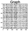
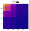
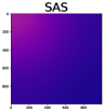
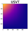
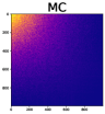
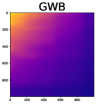
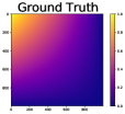
(a) $W(x,y)=xy$ and $0\leq x,y\leq 1$

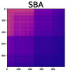
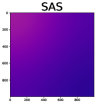
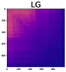
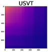
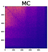
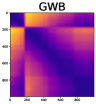
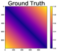
(b) $W(x,y)=|x-y|$ and $0\leq x,y\leq 1$

Figure 1: Illustrations of learning results obtained by various methods for different graphons. In both (a) and (b), we visualize the graphon and its estimations with size $1,000\times 1,000$, and each estimation is derived based on $10$ graphs with less than $300$ nodes. The node degrees of the graphs provide strong evidence to align graphs when learning the graphon in (a) but are useless for the graphon in (b). Our GWB method outperforms state-of-the-art methods. Especially in the challenging case (b), the estimation derived by our method can be aligned to the ground truth by a measure-preserving mapping, which is close to the ground truth under the cut distance.

These methods require the observed graphs to be well-aligned and generated by a single graphon. However, real-world graphs, $e.g.$, the social networks collected from different platforms and different time slots, often have complicated clustering structure, and the correspondence between their nodes is unknown in general. This violation limits the feasibility of the above learning methods in practice. Specifically, these methods have to solve a multi-graph matching problem before learning graphons. Because of the NP-hardness of the matching problem, this preprocessing often introduces severe noise to the subsequent learning problem and leads to undesirable learning results.

To overcome the aforementioned challenges, we propose a new method to learn one or multiple graphons from unaligned graphs. Our method leverages step functions to estimate graphons. It minimizes the Gromov-Wasserstein distance (GWD) (Mémoli 2011) between the step function of each observed graph and that of the target graphon, whose solution is a Gromov-Wasserstein barycenter (GWB) of the graphs (Xu, Luo, and Carin 2019). We demonstrate that this learning strategy minimizes an upper bound of the cut distance (Lovász 2012) between the graphon and its step function, which leads to a computationally-efficient algorithm.

To the best of our knowledge, our work makes the first attempt to learn graphons from unaligned graphs. Different from existing methods, which first match graphs heuristically and then estimate graphons, our method leverages the permutation-invariance of the GW distance and integrates graph matching implicitly in the estimation phase. As a result, our method mitigates bias caused by undesired matching processes. Given a graphon $W(x,y)$, if its marginal $W(y)=\int_{x\in\Omega}W(x,y)dx$ (or $W(x)=\int_{y\in\Omega}W(x,y)dy$) is very different from a constant function, the graphs generated by it can be aligned readily by sorting and matching their nodes according to their degrees. On the contrary, if its marginal is close to a constant function, it will be hard to align its graphs because the node degrees of the graphs’ nodes are almost the same. As illustrated in Figure 1, no matter whether it is easy to align the graphs or not, our method can successfully learn the graphons and consistently outperforms existing methods. Besides the basic GWB method, we design a smoothed GWB method to enhance the continuity of learned graphons. Additionally, to learn multiple graphons from the graphs with unknown clustering structures, we propose a mixture model of GWBs. These structured GWB models achieve encouraging learning results in some complicated scenarios.

Proposed Method

A graphon $W:\Omega^{2}\mapsto[0,1]$ is defined on a probability space $(\Omega,\mu)$, where $\mu$ is a probability measure on the space $\Omega$. Each $W$ formulates a space of graphons, denoted as $\mathcal{W}$. Let $\{\mathcal{G}_{m}\}_{m=1}^{M}$ be a set of graphs generated by an unknown graphon $W$, whose sampling process is shown in (1). We want to estimate the graphon based on the observed graphs, making the estimation close to the ground truth under a specific metric.

Approximate graphons by step functions

A graphon can always be approximated by a step function in the cut norm (Frieze and Kannan 1999). For each $W\in\mathcal{W}$, its cut norm is defined as

$$\begin{aligned} \|W\|_{\square}:=\sideset{}{{}_{\mathcal{X},\mathcal{Y}\subset\Omega}}{\sup}\Bigl{|}\int_{\mathcal{X}\times\mathcal{Y}}W(x,y)dxdy\Bigr{|},\end{aligned}$$ (2)

where the supremum is taken over all measurable subsets $\mathcal{X}$ and $\mathcal{Y}$ of $\Omega$. Based on the cut norm, we can define a commonly-used metric called cut distance (Lovász 2012) between $W_{1},W_{2}\in\mathcal{W}$:

$$\begin{aligned} \delta_{\square}(W_{1},W_{2}):=\sideset{}{{}_{\phi\in\mathcal{S}_{\Omega}}}{\inf}\|W_{1}-W_{2}^{\phi}\|_{\square},\end{aligned}$$ (3)

where $\mathcal{S}_{\Omega}$ represents the set of measure-preserving mappings from $\Omega$ to $\Omega$. Accordingly, we have $W_{2}^{\phi}(x,y)=W_{2}(\phi(x),\phi(y))$. The cut distance plays a central role in graphon theory. We say that two graphons $W_{1}$, $W_{2}$ are equivalent if $\delta_{\square}(W_{1},W_{2})=0$, denoted as $W_{1}\cong W_{2}$. The work in (Borgs et al. 2008) demonstrates that the quotient space $\widehat{\mathcal{W}}:=\mathcal{W}\setminus\cong$ is homeomorphic to the set of graphons and $(\widehat{\mathcal{W}},\delta_{\square})$ is a compact metric space. Similarly, we can define $\delta_{1}(W_{1},W_{2}):=\sideset{}{{}_{\phi\in\mathcal{S}_{\Omega}}}{\inf}\|W_{1}-W_{2}^{\phi}\|_{1}$, where $\|W\|_{1}:=\int_{\mathcal{X}\times\mathcal{Y}}|W(x,y)|dxdy$. According to their definitions, we have

$$\begin{aligned} \delta_{\square}(W_{1},W_{2})\leq\delta_{1}(W_{1},W_{2}),~{}\forall~{}W_{1},W_{2}\in\mathcal{W}.\end{aligned}$$ (4)

Let $\mathcal{P}=(\mathcal{P}_{1},..,\mathcal{P}_{K})$ be a partition of $\Omega$ into $K$ measurable sets. We define a step function $W_{\mathcal{P}}:\Omega^{2}\mapsto[0,1]$ as

$$\begin{aligned} W_{\mathcal{P}}(x,y)=\sideset{}{{}_{k,k^{\prime}=1}^{K}}{\sum}w_{kk^{\prime}}1_{\mathcal{P}_{k}\times\mathcal{P}_{k^{\prime}}}(x,y),\end{aligned}$$ (5)

where each $w_{kk^{\prime}}\in[0,1]$ and the indicator function $1_{\mathcal{P}_{k}\times\mathcal{P}_{k^{\prime}}}(x,y)$ is 1 if $(x,y)\in\mathcal{P}_{k}\times\mathcal{P}_{k^{\prime}}$, otherwise it is 0. The weak regularity lemma (Lovász 2012) shown below guarantees that every graphon can be approximated well in the cut norm by step functions.

Theorem 1 (Weak Regularity Lemma (Lovász 2012)).

For every graphon $W\in\mathcal{W}$ and $K\geq 1$, there always exists a step function $W_{\mathcal{P}}$ with $|\mathcal{P}|=K$ steps such that

$$\begin{aligned} \|W-W_{\mathcal{P}}\|_{\square}\leq\frac{2}{\sqrt{\log K}}\|W\|_{L_{2}}.\end{aligned}$$ (6)

Note that a corollary of this lemma is $\delta_{\square}(W,W_{\mathcal{P}})\leq\frac{2}{\sqrt{\log K}}\|W\|_{L_{2}}$ because $\delta_{\square}(W,W_{\mathcal{P}})\leq\|W-W_{\mathcal{P}}\|_{\square}$.

Oracle estimator

Based on the weak regularity lemma, we would like to learn a step function ${W}_{\mathcal{P}}$ from observed graphs $\{\mathcal{G}_{m}\}_{m=1}^{M}$ such that the cut distance between the step function and the ground truth, $i.e.$, $\delta_{\square}(W,{W}_{\mathcal{P}})$, is minimized. Note that a graph $\mathcal{G}$ can also be represented as a step function.

Definition 2.

For a graph with a node set $\mathcal{V}=\{1,...,N\}$ and an adjacency matrix $\bm{A}$, we can represent it as a step function with $N$ equitable partitions of $\Omega$, $i.e.$, $\mathcal{P}=\{\mathcal{P}_{n}\}_{n=1}^{N}$, denoted as $G_{\mathcal{P}}$, where $G_{\mathcal{P}}(x,y)=\frac{1}{N^{2}}\sum_{n,n^{\prime}=1}^{N}a_{nn^{\prime}}1_{\mathcal{P}_{n}\times\mathcal{P}_{n^{\prime}}}(x,y)$.

Ideally, if we know the positions of a graph’s nodes, $i.e.$, the $v_{n}$’s in (1), we can derive an isomorphism of the graph according to the order of the positions and obtain an “oracle” step function, denoted as $\hat{\mathcal{G}}$ and $\hat{G}_{\mathcal{P}}$, respectively. Applying this sorting operation to $\{\mathcal{G}_{m}\}_{m=1}^{M}$, we obtain a set of well-aligned graphs $\{\hat{\mathcal{G}}_{m}\}_{m=1}^{M}$ and a set of oracle step functions $\{\hat{G}_{m,\mathcal{P}^{m}}\}_{m=1}^{M}$, where the number of partitions $|\mathcal{P}^{m}|$ is equal to the number of nodes in $\hat{\mathcal{G}}_{m}$. Accordingly, we achieve an oracle estimator of $W$ as follows:

$$\begin{aligned} W_{O}=\frac{1}{M}\sideset{}{{}_{m=1}^{M}}{\sum}\hat{G}_{m,\mathcal{P}^{m}}.\end{aligned}$$ (7)

This oracle estimator provides a consistent estimation of $W$:

Theorem 3.

For every $W\in\mathcal{W}$, let $\{\hat{G}_{m,\mathcal{P}^{m}}\}_{m=1}^{M}$ be a set of oracle step functions defined by Definition 2. We have

$$\delta_{\square}(W,W_{O})\leq\frac{C}{\min_{m}|\mathcal{P}^{m}|},$$ (8)

where $C$ is a constant.

Proof.

For an arbitrary graphon $W$ and its oracle estimator $W_{O}$, we have

$$\begin{aligned} \delta_{\square}(W,W_{O})&=\delta_{\square}(W,\frac{1}{M}\sideset{}{{}_{m=1}^{M}}{\sum}\hat{G}_{m,\mathcal{P}^{m}})\\ &\leq\Bigl{\|}W-\frac{1}{M}\sideset{}{{}_{m=1}^{M}}{\sum}\hat{G}_{m,\mathcal{P}^{m}}\Bigr{\|}_{L_{2}}\\ &\leq\frac{1}{M}\sideset{}{{}_{m=1}^{M}}{\sum}\|W-\hat{G}_{m,\mathcal{P}^{m}}\|_{L_{2}}\\ &\leq\frac{1}{M}\sideset{}{{}_{m=1}^{M}}{\sum}\frac{C}{|\mathcal{P}^{m}|}\leq\frac{C}{\min_{m}|\mathcal{P}^{m}|}.\end{aligned}$$ (9)

The first inequality is based on the fact that for arbitrary two graphons, their cut distance is smaller than their $L_{2}$ distance (Janson 2013). The second inequality is the triangle inequality. The third inequality is a corollary of the step function approximation lemma in (Chan and Airoldi 2014), whose derivation corresponds to the second proof shown in the supplementary file of the reference. In particular, the constant $C$ corresponds to the supremum of the absolute difference between the graphon $W$ and its step function $\hat{G}$, which is independent of the number of partitions. ∎

Learning graphons via GW barycenters

The oracle estimator above is unavailable in practice because real-world graphs are generally unaligned – neither the positions of their nodes nor the correspondence between them is provided. Given such unaligned graphs, traditional learning methods first match observed graphs and then estimate the oracle step functions. As illustrated in Figure 1(b), this strategy often leads to failures because the matching step is NP-hard and creates wrongly-aligned graphs.

To mitigate the dependency on well-aligned graphs (and their oracle step functions), we propose a new learning strategy. Specifically, considering the oracle estimator, we have

$$\begin{aligned} &\delta_{\square}(W,W_{\mathcal{P}})\\ \leq&\delta_{\square}(W,W_{O})+\delta_{\square}(W_{O},W_{\mathcal{P}})\\ =&\delta_{\square}(W,W_{O})+\delta_{\square}(\frac{1}{M}\sideset{}{{}_{m=1}^{M}}{\sum}\hat{G}_{m,\mathcal{P}^{m}},W_{\mathcal{P}})\\ \leq&\delta_{\square}(W,W_{O})+\frac{1}{M}\sideset{}{{}_{m=1}^{M}}{\sum}\delta_{\square}(\hat{G}_{m,\mathcal{P}^{m}},W_{\mathcal{P}})\\ =&\delta_{\square}(W,W_{O})+\frac{1}{M}\sideset{}{{}_{m=1}^{M}}{\sum}\delta_{\square}(G_{m,\mathcal{P}^{m}},W_{\mathcal{P}})\\ \leq&\delta_{\square}(W,W_{O})+\frac{1}{M}\sideset{}{{}_{m=1}^{M}}{\sum}\delta_{1}(G_{m,\mathcal{P}^{m}},W_{\mathcal{P}}).\end{aligned}$$ (10)

The first inequality in (10) is the triangle inequality, and the second inequality is derived according to the definition of cut distance. The latter is manifested because $\delta_{\square}(G_{\mathcal{P}},\hat{G}_{\mathcal{P}})=0$ ($i.e.$, $G_{\mathcal{P}}\cong\hat{G}_{\mathcal{P}}$). Finally, the third inequality is based on (4). Theorem 3 and (10) indicate that we can minimize an upper bound of $\delta_{\square}(W,W_{\mathcal{P}})$ by solving the following optimization problem:

$$\begin{aligned} \sideset{}{{}_{W_{\mathcal{P}}}}{\min}\frac{1}{M}\sideset{}{{}_{m=1}^{M}}{\sum}\delta_{1}(G_{m,\mathcal{P}^{m}},W_{\mathcal{P}}).\end{aligned}$$ (11)

This strategy does not need to estimate the oracle step function, because it directly considers the $\delta_{1}$ distance between observed graphs and the proposed step function. To solve this problem, we derive a computationally-efficient alternative of $\delta_{1}$ based on its equivalent definition shown below.

Theorem 4 (Remark 6.13 in (Janson 2013)).

Let $W_{1}$ and $W_{2}$ be two graphons defined on the probability spaces $(\Omega_{1},\mu_{1})$ and $(\Omega_{2},\mu_{2})$, respectively. The $\delta_{1}(W_{1},W_{2})$ can be equivalently defined as $\inf_{\pi\in\Pi(\mu_{1},\mu_{2})}\int_{(\Omega_{1}\times\Omega_{2})^{2}}|W_{1}(x,y)-W_{2}(x^{\prime},y^{\prime})|d\pi(x,x^{\prime})d\pi(y,y^{\prime})$, where $\Pi(\mu_{1},\mu_{2})=\{\pi~{}|~{}\pi\geq 0,~{}\int_{y\in\Omega_{2}}d\pi(x,y)=\mu_{1},~{}\int_{x\in\Omega_{1}}d\pi(x,y)=\mu_{2}\}$ contains all measures on $\Omega_{1}\times\Omega_{2}$ having marginals $\mu_{1}$ and $\mu_{2}$.

The characterization shown in Theorem 4 coincides with the 1-order Gromov-Wasserstein distance between $(\Omega_{1},\mu_{1})$ and $(\Omega_{2},\mu_{2})$ (Mémoli 2011). Let $W_{1,\mathcal{P}}$ and $W_{2,\mathcal{Q}}$ be two step functions defined on $(\Omega_{1},\mu_{1})$ and $(\Omega_{2},\mu_{2})$, which have equitable partitions $\mathcal{P}=\{\mathcal{P}_{i}\}_{i=1}^{I}$ and $\mathcal{Q}=\{\mathcal{Q}_{j}\}_{j=1}^{J}$. We rewrite $W_{1}(x,y)-W_{2}(x^{\prime},y^{\prime})$ as $\sum_{i,j=1}^{I}w_{1,ij}1_{\mathcal{P}_{i}\times\mathcal{P}_{j}}(x,y)-\sum_{i^{\prime},j^{\prime}=1}^{J}w_{2,i^{\prime}j^{\prime}}1_{\mathcal{Q}_{i^{\prime}}\times\mathcal{Q}_{j^{\prime}}}(x^{\prime},y^{\prime})$ and denote $r_{iji^{\prime}j^{\prime}}$ as $|w_{1,ij}-w_{2,i^{\prime}j^{\prime}}|$. Let the probability measures $\mu_{1}$ and $\mu_{2}$ be constant in each partition, $i.e.$, $\mu_{1}(x)=\sum_{i}\mu_{1,i}1_{\mathcal{P}_{i}}(x)$ and $\mu_{2}(x)=\sum_{i}\mu_{2,j}1_{\mathcal{Q}_{j}}(x)$. We can then rewrite the $\delta_{1}$ distance between the two step functions as

$$\begin{aligned} &\delta_{1}(W_{1,\mathcal{P}},W_{2,\mathcal{Q}})\\ =&\inf_{\pi\in\Pi(\mu_{1},\mu_{2})}\sum_{i,i^{\prime},j,j^{\prime}}\int_{\mathcal{P}_{i}\times\mathcal{P}_{j}\times\mathcal{Q}_{i^{\prime}}\times\mathcal{Q}_{j^{\prime}}}r_{iji^{\prime}j^{\prime}}d\pi(x,x^{\prime})d\pi(y,y^{\prime})\\ =&\inf_{\pi\in\Pi({\mu}_{1},{\mu}_{2})}\sum_{i,i^{\prime},j,j^{\prime}}r_{iji^{\prime}j^{\prime}}\int_{\mathcal{P}_{i}\times\mathcal{Q}_{i^{\prime}}}d\pi(x,x^{\prime})\int_{\mathcal{P}_{j}\times\mathcal{Q}_{j^{\prime}}}d\pi(y,y^{\prime})\\ =&\sideset{}{{}_{\bm{T}\in\Pi(\bm{\mu}_{1},\bm{\mu}_{2})}}{\min}\sideset{}{{}_{i,i^{\prime},j,j^{\prime}}}{\sum}r_{iji^{\prime}j^{\prime}}T_{ii^{\prime}}T_{jj^{\prime}}=d_{\text{gw},1}(\bm{W}_{1},\bm{W}_{2}),\end{aligned}$$

where $\bm{W}_{1}=[w_{1,ij}]\in[0,1]^{I\times I}$ and $\bm{W}_{2}=[w_{2,i^{\prime}j^{\prime}}]\in[0,1]^{J\times J}$ rewrite the step functions in matrix form. Vectors $\bm{\mu}_{1}=[\mu_{1,i}]$ and $\bm{\mu}_{2}=[\mu_{2,j}]$ represents the probability measures $\mu_{1}$ and $\mu_{2}$; $\bm{T}=[T_{ii^{\prime}}]\in\mathbb{R}^{I\times J}$ is a doubly-stochastic matrix in the set $\Pi(\bm{\mu}_{1},\bm{\mu}_{2})=\{\bm{T}\geq\bm{0}|\bm{T}\bm{\mu}_{2}=\bm{\mu}_{1},\bm{T}^{\top}\bm{\mu}_{1}=\bm{\mu}_{2}\}$, whose element $T_{ii^{\prime}}=\int_{\mathcal{P}_{i}\times\mathcal{Q}_{i^{\prime}}}d\pi(x,x^{\prime})$. The optimal $\bm{T}$, denoted as $\bm{T}^{*}$, is called the optimal transport or optimal coupling between $\bm{\mu}_{1}$ and $\bm{\mu}_{2}$ (Villani 2008; Peyré, Cuturi, and others 2019).

The derivation above shows that instead of solving a complicated optimization problem in a function space, we can convert it to the 1-order Gromov-Wasserstein distance between matrices (Peyré, Cuturi, and Solomon 2016; Chowdhury and Mémoli 2019; Xu et al. 2019). Moreover, when we replace the $r_{iji^{\prime}j^{\prime}}$ with $r_{iji^{\prime}j^{\prime}}^{2}$, we obtain the squared 2-order Gromov-Wasserstein distance:

$$\begin{aligned} d_{\text{gw},2}^{2}(\bm{W}_{1},\bm{W}_{2})=&\sideset{}{}{\min}_{\bm{T}\in\Pi(\bm{\mu}_{1},\bm{\mu}_{2})}\sideset{}{{}_{i,i^{\prime},j,j^{\prime}}}{\sum}r_{iji^{\prime}j^{\prime}}^{2}T_{ii^{\prime}}T_{jj^{\prime}}\\ =&\sideset{}{{}_{\bm{T}\in\Pi(\bm{\mu}_{1},\bm{\mu}_{2})}}{\min}\langle\bm{D}-2\bm{W}_{1}\bm{T}\bm{W}_{2}^{\top},\bm{T}\rangle.\end{aligned}$$ (12)

Here, $\langle\cdot,\cdot\rangle$ calculates the inner product of two matrices. $\bm{D}=(\bm{W}_{1}\odot\bm{W}_{1})\bm{\mu}_{1}\bm{1}_{J}^{\top}+\bm{1}_{I}\bm{\mu}_{2}^{\top}(\bm{W}_{2}\odot\bm{W}_{2})$, where $\bm{1}_{I}$ is an $I$-dimensional all-one vector and $\odot$ represents the Hadamard product of matrix. Because the 2-order GW distance and the 1-order GW distance are equivalent (pseudo) metrics (Theorem 5.1 in (Mémoli 2011)), the $d_{\text{gw},2}^{2}(\bm{W}_{1},\bm{W}_{2})$ also provides a good alternative for the cut distance of the step functions. Plugging (12) into (11), the learning problem becomes estimating a GW barycenter of the observed graphs (Peyré, Cuturi, and Solomon 2016):

$$\begin{aligned} \sideset{}{{}_{\bm{W}\in[0,1]^{K\times K}}}{\min}\frac{1}{M}\sideset{}{{}_{m=1}^{M}}{\sum}d^{2}_{\text{gw},2}(\bm{A}_{m},\bm{W}),\end{aligned}$$ (13)

where $\bm{A}_{m}$ is the adjacency matrix of the graph $\mathcal{G}_{m}$ and $\bm{W}=[w_{kk^{\prime}}]\in[0,1]^{K\times K}$ is the matrix representation of step function $W_{\mathcal{P}}$. Note that the number of partitions $K$ and the probability measures associated with $\bm{W}$ and $\{\bm{A}_{m}\}_{m=1}^{N}$ are predefined. In the following subsection, we detail how to solve (13).

Implementation details

Setting the number of partitions Given a set of graphs $\{\mathcal{G}_{m}\}_{m}^{M}$, we denote $N_{\max}$ as the number of the nodes of the largest graph. Following the work in (Chan and Airoldi 2014; Airoldi, Costa, and Chan 2013; Channarond et al. 2012), we can set the number of partitions to be $K=\lfloor\frac{N_{\max}}{\log N_{\max}}\rfloor$. This setting has been proven helpful to achieve a trade-off between accuracy and computational efficiency.

Estimating probability measures For the observed graphs, we estimate the probability measures by normalized node degrees (Xu, Luo, and Carin 2019). We assume that the probability measure of $\bm{W}$ is sorted, $i.e.$, $\bm{\mu}_{W}=[\mu_{W,1},...,\mu_{W,K}]$ and $\mu_{W,1}\geq...\geq\mu_{W,K}$, which is estimated by sorting and merging $\{\bm{\mu}_{m}\}_{m=1}^{M}$. Here, $\bm{\mu}_{m}=\frac{1}{\|\bm{A}_{m}\bm{1}_{N_{m}}\|_{1}}\bm{A}_{m}\bm{1}_{N_{m}}$ for $m=1,...,M$, and

$$\begin{aligned} \bm{\mu}_{W}=\frac{1}{M}\sideset{}{{}_{m=1}^{M}}{\sum}\text{interp1d}_{K}(\text{sort}(\bm{\mu}_{m})),\end{aligned}$$ (14)

where $\text{sort}(\cdot)$ sorts the elements of the input vector in descending order, and $\text{interp1d}_{K}(\cdot)$ samples $K$ values from the input vector via linear interpolation. This strategy has proven beneficial for calculating the GW distance between graphs, which provides useful information when calculating the optimal transport between each $\bm{A}_{m}$ and the $\bm{W}$ (Xu, Luo, and Carin 2019).

Learning optimal transports The computation of the $d_{\text{gw},2}^{2}(\bm{A}_{m},\bm{W})$ is a non-convex, non-smooth optimization problem. To solve this problem efficiently, we apply the proximal gradient algorithm developed in (Xu et al. 2019). This algorithm reformulates the original problem as a series of subproblems and solves them iteratively. In each iteration, the subproblem is

$$\min_{\bm{T}\in\Pi(\bm{\mu}_{m},\bm{\mu}_{W})}\langle\bm{D}_{m}-2\bm{A}_{m}\bm{T}^{(s)}\bm{W}^{\top},\bm{T}\rangle+\beta\text{KL}(\bm{T}\lVert\bm{T}^{(s)}),$$ (15)

where $\bm{T}^{(s)}$ is the previous estimation of $\bm{T}$, $\bm{D}_{m}=(\bm{A}_{m}\odot\bm{A}_{m})\bm{\mu}_{m}\bm{1}_{K}+\bm{1}_{N_{m}}\bm{\mu}_{W}^{\top}(\bm{W}\odot\bm{W})$. We fix one transport matrix as its previous estimation in the GW term and add a proximal term as the regularizer. Here, the proximal term penalizes the KL-divergence between the transport matrix and its previous estimation, which smooths the update of the transport matrix. This problem can be solved by the Sinkhorn scaling algorithm (Sinkhorn and Knopp 1967), whose convergence rate is linear (Altschuler, Weed, and Rigollet 2017; Xie et al. 2020).

Learning GW barycenters Given the optimal transports $\{\bm{T}_{m}\}_{m=1}^{M}$, the GW barycenter has a closed-form solution (Peyré, Cuturi, and Solomon 2016):

$$\bm{W}=\frac{1}{\bm{\mu}_{W}\bm{\mu}_{W}^{T}}\sideset{}{{}_{m=1}^{M}}{\sum}\bm{T}_{m}^{\top}\bm{A}_{m}\bm{T}_{m}.$$ (16)

The scheme of our algorithm is shown in Algorithm 1.

Algorithm 1 Learning Graphons via GWB

1:  Input: Adjacency matrices $\{\bm{A}_{m}\}_{m=1}^{M}$. The weight of proximal term $\beta$, the number of iterations $L$, the number of inner Sinkhorn iterations $S$.

2:  Initialize $K=\lfloor\frac{N_{\max}}{\log N_{\max}}\rfloor$, and $\bm{W}\sim\text{Uniform}([0,1])$.

3:  Initialize $\{\bm{\mu}_{m}\}_{m=1}^{M}$ and $\bm{\mu}_{W}$ via (14)

4:  For $l=1,...,L$:

5:   For $m=1,...,M$:// Solve (15)

6:    Initialize $\bm{T}^{(0)}=\bm{\mu}_{m}\bm{\mu}_{W}^{\top}$ and $\bm{a}=\bm{\mu}_{m}$.

7:    For $s=0,...,S-1$:

8:     $\bm{C}=\exp(-\frac{1}{\beta}(\bm{D}_{m}-2\bm{A}_{m}\bm{T}^{(s)}\bm{W}^{\top}))\odot\bm{T}^{(s)}$

9:     $\bm{b}=\frac{\bm{\mu}_{W}}{\bm{C}^{\top}\bm{a}}$, $\bm{a}=\frac{\bm{\mu}_{m}}{\bm{C}\bm{b}}$, $\bm{T}^{(s+1)}=\text{diag}(\bm{a}){\bm{C}}\text{diag}(\bm{b})$.

10:    $\bm{T}_{m}=\bm{T}^{(S)}$.

11:   Update $\bm{W}$ via (16).

12:  The graphon $W_{\bm{P}}(x,y)=\sum_{k,k^{\prime}}w_{kk^{\prime}}1_{\bm{P}_{k}\times\bm{P}_{k^{\prime}}}(x,y)$.

Structured Gromov-Wasserstein Barycenters

We extend the above algorithm and propose two kinds of structured Gromov-Wasserstein barycenters to apply our learning method to more complicated scenarios.

Smoothed GW Barycenters As shown in Figure 1(b), the estimated graphons achieved by our method can be discontinuous because of the permutation invariance of Gromov-Wasserstein distance. To suppress the discontinuity of the results, we impose a smoothness regularization on the GW barycenters and obtain the following problem:

$$\begin{aligned} \sideset{}{{}_{\bm{W}\in[0,1]^{K\times K}}}{\min}&\frac{1}{M}\sideset{}{{}_{m=1}^{M}}{\sum}\langle\bm{D}_{m}-2\bm{A}_{m}\bm{T}_{m}\bm{W}^{\top},\bm{T}_{m}\rangle\\ &+\alpha\|\bm{L}\bm{W}\bm{L}^{\top}\|_{F}^{2},\end{aligned}$$ (17)

where $\bm{T}_{m}$ is current estimation of the $m$-th optimal transport and $\bm{L}\bm{W}\bm{L}^{\top}$ is the matrix representation of the Laplacian filtering of $\bm{W}$. The first-order optimality condition of this problem also has a closed-form solution. In particular, setting the gradient of the objection to zero, we obtain

$$\begin{aligned} &2\alpha\bm{L}^{\top}\bm{L}\bm{W}\bm{L}^{\top}\bm{L}+\text{diag}(\bm{\mu}_{W})\bm{W}\text{diag}(\bm{\mu}_{W})\\ =&\frac{1}{M}\sideset{}{{}_{m=1}^{M}}{\sum}\bm{T}_{m}^{\top}\bm{A}_{m}\bm{T}_{m}.\end{aligned}$$ (18)

Applying singular value decomposition (SVD) to $\bm{L}^{\top}\bm{L}$, $i.e.$, $\bm{L}^{\top}\bm{L}=\bm{U}\bm{\Lambda}\bm{U}^{\top}$, we rewrite the left side of (18) as $\bm{H}\bm{W}\bm{H}^{H}$, where $\bm{H}=\bm{U}(\sqrt{2\alpha}\bm{\Lambda}+i\text{diag}(\bm{\mu}_{W}))\bm{U}^{\top}$ is a symmetric complex matrix and $\bm{H}^{H}=\bm{U}(\sqrt{2\alpha}\bm{\Lambda}-i\text{diag}(\bm{\mu}_{W}))\bm{U}^{\top}$ is its Hermitian transpose. Therefore, we obtain a smoothed $\bm{W}$ by replacing line 11 of Algorithm 1 with $\bm{W}=\frac{1}{M}\bm{H}^{-1}\left(\sideset{}{{}_{m=1}^{M}}{\sum}\bm{T}_{m}^{\top}\bm{A}_{m}\bm{T}_{m}\right)\bm{H}^{-H}$.

Mixed GW Barycenters When the observed graphs are generated by $C$ different graphons, we can build a graphon mixture model and learn it as mixed GW barycenters:

$$\begin{aligned} \min_{\{\bm{W}_{c}\}_{c=1}^{C},\bm{P}\in\Pi(\frac{1}{C}\bm{1}_{C},\frac{1}{M}\bm{1}_{M})}\sideset{}{}{\sum}_{c=1}^{C}\sideset{}{}{\sum}_{m=1}^{M}p_{cm}d^{2}_{\text{gw},2}(\bm{A}_{m},\bm{W}_{c}).\end{aligned}$$ (19)

where we set $\bm{P}=[p_{cm}]$ as a doubly stochastic matrix, whose marginals are $\frac{1}{C}\bm{1}_{C}$ and $\frac{1}{M}\bm{1}_{M}$. The value $p_{cm}$ indicates the joint probability that the $m$-th graph is generated by the $c$-th graphon. In other words, the objective function of (19) leads to a hierarchical optimal transport problem (Luo, Xu, and Carin 2020), in which the ground distance is defined by the GW distance and $\bm{P}$ is the optimal transport matrix. This problem is solved by alternating optimization. In particular, replacing $\frac{1}{M}$ with $p_{cm}$, we still apply Algorithm 1 to learn $\{\bm{W}_{c}\}_{c=1}^{C}$. Given $\{\bm{W}_{c}\}_{c=1}^{C}$, we calculate the ground distance matrix $\bm{D}_{\text{gw}}=[d^{2}_{\text{gw},2}(\bm{A}_{m},\bm{W}_{c})]$ and update $\bm{P}$ by solving an optimal transport problem with an entropy regularization.

$$\begin{aligned} \sideset{}{{}_{\bm{P}\in\Pi(\frac{1}{C}\bm{1}_{C},\frac{1}{M}\bm{1}_{M})}}{\min}\langle\bm{D}_{\text{gw}},\bm{P}\rangle+\beta\langle\bm{P},\log\bm{P}\rangle.\end{aligned}$$ (20)

Similar to (15), this problem can also be solved by the Sinkhorn scaling algorithm in (Sinkhorn and Knopp 1967).

Related Work

Graphon estimation As a classic graphon estimation method, the stochastic block approximation (SBA) learns stochastic block models as graphons (Airoldi, Costa, and Chan 2013). The block size of the method can be optimized heuristically by the “largest gap” algorithm (Channarond et al. 2012). The smoothing-and-sorting (SAS) method improves this strategy by adding total-variation denoising as a post-processing step (Chan and Airoldi 2014). The work in (Pensky and others 2019) further extends this strategy and proposes a dynamic stochastic block model to describe time-varying graphons. The matrix completion (MC) method (Keshavan, Montanari, and Oh 2010), the universal singular value thresholding (USVT) algorithm (Chatterjee and others 2015), and the spectral method (Xu 2018) learn low-rank matrices as the proposed step functions. The work in (Ruiz, Chamon, and Ribeiro 2020) represents graphons by their Fourier transformations. The methods above require that the observed graphs be well-aligned and generated by a single graphon. Our work makes the first attempt to learn one or multiple graphons from unaligned graphs.

Table 1: Comparisons on estimation errors (MSE for “Easy to align”, $d_{\text{gw},2}$ for “Hard to align”)

Type	$W(x,y)$, $x,y\in[0,1]$	# nodes	SBA	LG	MC	USVT	SAS	GWB	SGWB
	$xy$	$200$	65.6$\pm$6.5	29.8$\pm$5.7	11.3$\pm$0.8	31.7$\pm$2.5	125.0$\pm$1.3	40.6$\pm$5.7	39.3$\pm$5.5
		100$\sim$300	157.4$\pm$23.3	133.2$\pm$22.8	138.3$\pm$21.3	131.2$\pm$24.2	161.9$\pm$19.5	52.5$\pm$13.1	51.9$\pm$12.6
	$e^{-(x^{0.7}+y^{0.7})}$	$200$	58.7$\pm$7.8	22.9$\pm$3.1	71.7$\pm$0.5	12.2$\pm$1.5	77.7$\pm$0.8	21.6$\pm$2.1	20.9$\pm$1.8
		100$\sim$300	165.2$\pm$22.8	157.6$\pm$24.2	166.2$\pm$21.5	158.2$\pm$24.5	153.4$\pm$25.1	48.6$\pm$11.9	48.0$\pm$10.8
	$\frac{x^{2}+y^{2}+\sqrt{x}+\sqrt{y}}{4}$	$200$	63.4$\pm$7.6	24.1$\pm$2.5	73.2$\pm$0.7	33.8$\pm$1.1	99.3$\pm$1.2	18.9$\pm$3.5	18.4$\pm$2.8
		100$\sim$300	258.5$\pm$36.0	254.2$\pm$36.6	259.5$\pm$35.0	254.2$\pm$36.8	240.6$\pm$39.2	81.0$\pm$18.8	80.5$\pm$17.8
Easy	$\frac{1}{2}(x+y)$	$200$	66.2$\pm$8.3	24.0$\pm$2.5	71.9$\pm$0.6	40.2$\pm$0.8	108.3$\pm$1.0	21.2$\pm$4.6	20.2$\pm$3.9
		100$\sim$300	247.6$\pm$40.3	241.3$\pm$41.0	247.0$\pm$39.1	241.3$\pm$41.0	231.3$\pm$40.2	83.8$\pm$22.5	84.6$\pm$22.0
to	$\frac{1}{1+\exp(-10(x^{2}+y^{2}))}$	$200$	55.0$\pm$9.5	23.1$\pm$3.2	64.6$\pm$0.5	37.3$\pm$0.6	73.3$\pm$0.7	14.8$\pm$2.3	16.1$\pm$1.5
		100$\sim$300	394.0$\pm$45.7	397.0$\pm$46.5	400.7$\pm$45.6	399.3$\pm$47.0	345.4$\pm$52.6	62.8$\pm$12.6	62.5$\pm$12.3
Align	$\frac{1}{1+\exp(-(\max\{x,y\}^{2}}$	$200$	48.3$\pm$6.1	24.5$\pm$2.3	71.1$\pm$0.4	24.4$\pm$0.5	54.4$\pm$0.5	15.3$\pm$1.0	17.1$\pm$1.4
		100$\sim$300	382.9$\pm$54.7	387.9$\pm$53.6	392.5$\pm$52.3	391.9$\pm$54.8	336.7$\pm$58.6	39.8$\pm$8.6	41.7$\pm$8.3
(MSE)	$e^{-\max\{x,y\}^{3/4}}$	$200$	56.3$\pm$7.1	26.8$\pm$0.9	79.3$\pm$0.5	50.6$\pm$0.3	68.6$\pm$0.6	21.4$\pm$1.7	21.2$\pm$1.0
		100$\sim$300	234.7$\pm$32.9	234.0$\pm$33.3	241.4$\pm$31.2	242.9$\pm$33.3	212.0$\pm$36.5	49.3$\pm$9.5	48.7$\pm$9.1
	$e^{-\frac{\min\{x,y\}+\sqrt{x}+\sqrt{y}}{2}}$	$200$	55.7$\pm$7.7	26.4$\pm$5.6	76.4$\pm$0.4	28.3$\pm$0.5	76.4$\pm$0.8	23.2$\pm$1.3	23.3$\pm$1.4
		100$\sim$300	232.1$\pm$30.8	231.4$\pm$31.8	238.7$\pm$29.9	232.6$\pm$31.9	208.3$\pm$34.8	48.2$\pm$11.7	47.9$\pm$11.0
	$\log(1+\max\{x,y\})$	$200$	66.0$\pm$8.4	37.1$\pm$6.6	66.9$\pm$0.8	120.9$\pm$0.5	137.0$\pm$1.2	23.7$\pm$2.5	23.2$\pm$1.8
		100$\sim$300	370.8$\pm$38.9	370.7$\pm$40.4	374.5$\pm$39.5	375.5$\pm$37.5	337.7$\pm$42.1	104.0$\pm$18.8	107.4$\pm$18.9
Hard	$|x-y|$	$200$	0.202$\pm$0.001	0.200$\pm$0.002	0.206$\pm$0.001	0.215$\pm$0.002	0.217$\pm$0.002	0.057$\pm$0.005	0.050$\pm$0.003
		100$\sim$300	0.254$\pm$0.007	0.254$\pm$0.008	0.254$\pm$0.009	0.261$\pm$0.009	0.248$\pm$0.008	0.085$\pm$0.012	0.080$\pm$0.010
to	$1-|x-y|$	$200$	0.200$\pm$0.001	0.198$\pm$0.002	0.202$\pm$0.002	0.209$\pm$0.003	0.217$\pm$0.001	0.063$\pm$0.003	0.057$\pm$0.001
		100$\sim$300	0.383$\pm$0.041	0.384$\pm$0.040	0.383$\pm$0.040	0.393$\pm$0.041	0.350$\pm$0.044	0.075$\pm$0.009	0.077$\pm$0.004
Align	$0.8\bm{I}_{2}\otimes 1_{[0,\frac{1}{2}]^{2}}$	$200$	0.252$\pm$0.018	0.258$\pm$0.018	0.258$\pm$0.016	0.252$\pm$0.016	0.367$\pm$0.004	0.252$\pm$0.002	0.218$\pm$0.001
		100$\sim$300	0.355$\pm$0.005	0.359$\pm$0.002	0.361$\pm$0.005	0.392$\pm$0.038	0.409$\pm$0.004	0.328$\pm$0.034	0.329$\pm$0.032
($d_{\text{gw},2}$)	$0.8\text{flip}(\bm{I}_{2})\otimes 1_{[0,\frac{1}{2}]^{2}}$	$200$	0.241$\pm$0.010	0.254$\pm$0.005	0.250$\pm$0.003	0.242$\pm$0.003	0.364$\pm$0.001	0.252$\pm$0.002	0.190$\pm$0.058
		100$\sim$300	0.453$\pm$0.004	0.487$\pm$0.002	0.450$\pm$0.008	0.477$\pm$0.001	0.468$\pm$0.001	0.427$\pm$0.027	0.420$\pm$0.027

Gromov-Wasserstein distance The GW distance has been widely used to measure the difference between structured data, $e.g.$, geometry shapes (Mémoli 2011) and graphs (Vayer et al. 2018). For graphs, the optimal transport associated with their GW distance indicates the correspondence between their nodes, which is beneficial for graph matching (Xu et al. 2019). To calculate this distance, the work in (Peyré, Cuturi, and Solomon 2016) adds an entropy regularizer to the objective function and applies the Sinkhorn scaling algorithm (Cuturi 2013). The work in (Xu et al. 2019) improves this method by replacing the entropy regularizer with a Bregman proximal term. An ADMM-based method is proposed in (Xu 2020) to calculate the GW distance between directed graphs. Recently, the recursive GW distance (Xu, Luo, and Carin 2019) and the sliced GW distance (Titouan et al. 2019b) have been proposed to reduce the computational complexity of the GW distance. A GW barycenter model is proposed in (Peyré, Cuturi, and Solomon 2016), which shows the potential of graph clustering (Xu 2020). Our work is pioneering in the development of structured GW barycenters to learn graphons.

Experiments

Synthetic data

To demonstrate the efficacy of our GWB method and its smoothed variant (SGWB), we compare them with existing methods on learning synthetic graphons. We set the hyperparameters of our methods as follows: the weight of the proximal term $\beta=0.005$, the number of iterations $L=5$, and the number of Sinkhorn iterations $S=10$; for the SGWB method, the weight of the smoothness regularizer $\alpha=0.0002$. The baselines include the stochastic block approximation (SBA) (Airoldi, Costa, and Chan 2013), the “largest gap” (LG) based block approximation (Channarond et al. 2012), the matrix completion (MC) (Keshavan, Montanari, and Oh 2010), the universal singular value thresholding (USVT) (Chatterjee and others 2015), and the sorting-and-smoothing (SAS) (Chan and Airoldi 2014).

We prepare 13 kinds of synthetic graphons, whose definitions are shown in Table 1. The resolution of these graphons is $1000\times 1000$. Among these graphons, nine are considered in (Chan and Airoldi 2014). The graphs generated by them are easy to align – the node degrees of these graphs provide strong evidence to sort and match nodes. For these graphons, we apply the mean-square-error (MSE) to evaluate different methods. Additionally, to highlight the advantage of our method, we design four challenging graphons, whose graphs are hard to align. In particular, for the graphs generated by these four graphons, the node degrees of different nodes can be equal to each other. Therefore, there is no simple way of aligning the graphs. For these graphons, we apply the GW distance $d_{\text{gw},2}$ as the evaluation measurement. For each graphon, we simulate graphs with two different settings: In one setting, each of the graphs has $200$ nodes, while in the other setting, the number of each graph’s nodes is sampled uniformly from the range $[100,300]$. Originally, the baselines above are designed for the former setting. When dealing with graphs with different sizes, they pad zeros to the corresponding adjacency matrices and enforce the graphs to have the same size. For each setting, we test our method and the baselines in $10$ trials, and in each trial we simulate $10$ graphs and estimate the graphon by different methods.

Table 2: Comparisons on averaged MSE and runtime (second) under different configurations

Measurement	# graphs $M$	# nodes $N$	SBA	LG	MC	USVT	SAS	GWB	SGWB
MSE	2	200	62.1$\pm$9.0	26.5$\pm$3.9	73.6$\pm$2.3	45.6$\pm$1.6	94.1$\pm$1.5	24.6$\pm$4.3	24.3$\pm$3.3
	10	200	59.5$\pm$7.7	26.5$\pm$3.6	70.7$\pm$0.6	39.9$\pm$0.9	91.1$\pm$0.9	22.3$\pm$2.8	21.9$\pm$2.4
	20	200	32.2$\pm$2.0	23.7$\pm$4.1	50.7$\pm$0.4	38.7$\pm$0.5	91.0$\pm$0.7	21.1$\pm$2.0	20.7$\pm$1.7
	2	500	59.4$\pm$0.4	49.1$\pm$2.0	69.0$\pm$1.8	35.4$\pm$2.4	23.9$\pm$4.3	22.2$\pm$7.0	21.1$\pm$4.5
	10	500	47.1$\pm$5.6	20.2$\pm$1.4	60.6$\pm$0.3	27.6$\pm$0.4	34.8$\pm$0.8	19.7$\pm$2.5	19.6$\pm$1.7
	20	500	34.1$\pm$3.3	18.8$\pm$1.7	43.2$\pm$0.2	27.0$\pm$0.3	35.4$\pm$0.7	17.3$\pm$1.9	17.7$\pm$1.4
Runtime	10	200	0.69$\pm$0.03	0.61$\pm$0.04	0.02$\pm$0.01	0.02$\pm$0.00	0.03$\pm$0.01	0.32$\pm$0.04	0.34$\pm$0.03
	10	500	3.74$\pm$0.09	3.69$\pm$0.08	0.08$\pm$0.02	0.09$\pm$0.01	0.08$\pm$0.01	0.67$\pm$0.06	0.70$\pm$0.06

The experimental results in Table 1 show that our GWB method outperforms the baselines in most situations. Especially for the graphs that are hard to align, the gap between our methods and the baselines become bigger. When the observed graphs have different sizes, the estimation errors of the baselines increase because the padding step does harm to the alignment of the graphs. By contrast, our GWB method is relatively robust to the variance of graph size, and it achieves much lower estimation errors. Additionally, with the help of the smoothness regularizer, our SGWB method improves the stability of the original GWB method, which achieves comparable estimator errors but with smaller standard deviations. Typical visualization results are shown in Figure 1.

Moreover, our methods are robust across datasets. In particular, for the nine graphons that are easy to align, we generate different numbers of graphs with different sizes. Under each configuration, we record the averaged MSEs of the learning methods in Table 2, which verifies the robustness of our method.

Besides estimation errors, we also compare various methods on their computational complexity. Suppose that we have $M$ graphs, and each of them has $N$ nodes and $E$ edges. Learning a step function with $K$ partitions as a graphon, we list the complexity of the methods in Table 3. In particular, line 8 of Algorithm 1 involves sparse matrix multiplication, whose complexity is $\mathcal{O}(EK+NK^{2})$. Because the graphs often have sparse edges, $i.e.$, $E=\mathcal{O}(N\log N)$ and $K=\mathcal{O}(\frac{N}{\log N})$, the complexity of our GWB method is comparable to others when the numbers of iterations ($i.e.$, $L$ and $S$) are small. The runtime in Table 2 shows that our GWB and SGWB are generally faster than SBA and LG in practice.

Table 3: Comparisons on computational complexity

Method	Complexity	Method	Complexity
LG	$\mathcal{O}(MN^{2})$	SBA	$\mathcal{O}(MKN\log N)$
MC	$\mathcal{O}(N^{3})$	SAS	$\mathcal{O}(MN\log N+K^{2}\log K^{2})$
USVT	$\mathcal{O}(N^{3})$	GWB	$\mathcal{O}(LSM(EK+NK^{2}))$

Real-world data

For real-world graph datasets, our mixed GWB method (MixGWBs) provides a new way to cluster graphs. In particular, by learning $C$ graphons from $M$ graphs, we achieve $C$ centroids of different clusters and the learned optimal transport $\bm{P}=[p_{cm}]$ indicates the probability that the $m$-th graph belongs to the $c$-th cluster. To demonstrate the effectiveness of our method, we test it on two datasets and compare it with three baselines. The datasets are the IMDB-BINARY and the IMDB-MULTI (Yanardag and Vishwanathan 2015), which can be downloaded from (Morris et al. 2020). The IMDB-BINARY contains 1000 graphs belonging to two clusters, while the IMDB-MULTI contains 1500 graphs belonging to three clusters. These two datasets are challenging for graph clustering, as the nodes and edges of their graphs do not have any side information. We have to cluster graphs merely based on their binary adjacency matrices.

For these two datasets, the clustering methods based on the GW distance achieve state-of-the-art performance. The representative methods include ($i$) the fused Gromov-Wasserstein kernel method (FGWK) (Titouan et al. 2019a); ($ii$) the K-means using the Gromov-Wasserstein distance as the metric (GW-KM); and ($iii$) the Gromov-Wasserstein factorization (GWF) method (Xu 2020). We test our MixGWBs method and compare it with these three methods on clustering accuracy. In particular, for each dataset, we apply 10-fold cross-validation to evaluate each clustering method. The averaged clustering accuracy and the standard deviation are shown in Table 4. The performance of our method is at least comparable to that of the competitors. Figure 2 visualizes the graphons learned by our method and illustrates the difference between different clusters. We can find that the graphons correspond to the block models with different block sizes. Additionally, the IMDB-MULTI is much more challenging than the IMDB-BINARY, because it contains three rather than two clusters and the block structure of each cluster is not so clear as the clusters of the IMDB-BINARY.

Table 4: Comparisons on clustering accuracy (%)

Dataset	FGWK	GW-KM	GWF	MixGWBs
IMDB-BINARY	56.7$\pm$1.5	53.5$\pm$2.3	60.6$\pm$1.7	61.4$\pm$1.8
IMDB-MULTI	42.3$\pm$2.4	41.0$\pm$3.1	40.8$\pm$2.0	42.9$\pm$1.9

(a) IMDB-BINARY

(b) IMDB-MULTI

Figure 2: Illustrations of estimated graphons.

Conclusions

In this paper, we propose a novel method to learn graphons from unaligned graphs. Our method minimizes an upper bound of the cut distance between the target graphons and their approximations, which leads to a GW barycenter problem. To extend our method to practical scenarios, we developed two structured variants of the basic GWB algorithm. In the future, we plan to improve the robustness of our method to the weight of the smoothness regularizer and further reduce the complexity of our method by applying the recursive GW distance (Xu, Luo, and Carin 2019) or the sliced GW distance (Titouan et al. 2019b) to accelerate the computation of optimal transports. Additionally, because the graphon is naturally a generative graph model, we will consider using the model to achieve graph generation tasks.

References

- Airoldi, Costa, and Chan (2013) Airoldi, E. M.; Costa, T. B.; and Chan, S. H. 2013. Stochastic blockmodel approximation of a graphon: Theory and consistent estimation. In Advances in Neural Information Processing Systems, 692–700.
- Altschuler, Weed, and Rigollet (2017) Altschuler, J.; Weed, J.; and Rigollet, P. 2017. Near-linear time approximation algorithms for optimal transport via Sinkhorn iteration. In Advances in Neural Information Processing Systems, 1964–1974.
- Avella-Medina et al. (2018) Avella-Medina, M.; Parise, F.; Schaub, M.; and Segarra, S. 2018. Centrality measures for graphons: Accounting for uncertainty in networks. IEEE Transactions on Network Science and Engineering.
- Ballester, Calvó-Armengol, and Zenou (2006) Ballester, C.; Calvó-Armengol, A.; and Zenou, Y. 2006. Who’s who in networks. Wanted: The key player. Econometrica 74:1403–1417.
- Borgs et al. (2008) Borgs, C.; Chayes, J. T.; Lovász, L.; Sós, V. T.; and Vesztergombi, K. 2008. Convergent sequences of dense graphs I: Subgraph frequencies, metric properties and testing. Advances in Mathematics 219(6):1801–1851.
- Chan and Airoldi (2014) Chan, S., and Airoldi, E. 2014. A consistent histogram estimator for exchangeable graph models. In International Conference on Machine Learning, 208–216.
- Channarond et al. (2012) Channarond, A.; Daudin, J.-J.; Robin, S.; et al. 2012. Classification and estimation in the stochastic blockmodel based on the empirical degrees. Electronic Journal of Statistics 6:2574–2601.
- Chatterjee and others (2015) Chatterjee, S., et al. 2015. Matrix estimation by universal singular value thresholding. The Annals of Statistics 43(1):177–214.
- Chowdhury and Mémoli (2019) Chowdhury, S., and Mémoli, F. 2019. The gromov-Wasserstein distance between networks and stable network invariants. Information and Inference: A Journal of the IMA 8(4):757–787.
- Chung and Radcliffe (2011) Chung, F., and Radcliffe, M. 2011. On the spectra of general random graphs. the electronic journal of combinatorics P215–P215.
- Cuturi (2013) Cuturi, M. 2013. Sinkhorn distances: Lightspeed computation of optimal transport. In Advances in neural information processing systems, 2292–2300.
- Frieze and Kannan (1999) Frieze, A., and Kannan, R. 1999. Quick approximation to matrices and applications. Combinatorica 19(2):175–220.
- Gao and Caines (2019) Gao, S., and Caines, P. E. 2019. Graphon control of large-scale networks of linear systems. IEEE Transactions on Automatic Control.
- Goldenberg et al. (2010) Goldenberg, A.; Zheng, A. X.; Fienberg, S. E.; and Airoldi, E. M. 2010. A survey of statistical network models. Foundations and Trends® in Machine Learning 2(2):129–233.
- Hoff, Raftery, and Handcock (2002) Hoff, P. D.; Raftery, A. E.; and Handcock, M. S. 2002. Latent space approaches to social network analysis. Journal of the american Statistical association 97(460):1090–1098.
- Jackson and Zenou (2015) Jackson, M. O., and Zenou, Y. 2015. Games on networks. In Handbook of game theory with economic applications, volume 4. Elsevier. 95–163.
- Janson and Diaconis (2008) Janson, S., and Diaconis, P. 2008. Graph limits and exchangeable random graphs. Rendiconti di Matematica e delle sue Applicazioni. Serie VII 33–61.
- Janson (2013) Janson, S. 2013. Graphons, cut norm and distance, couplings and rearrangements. New York journal of mathematics.
- Keshavan, Montanari, and Oh (2010) Keshavan, R. H.; Montanari, A.; and Oh, S. 2010. Matrix completion from a few entries. IEEE transactions on information theory 56(6):2980–2998.
- Kolaczyk (2009) Kolaczyk, E. D. 2009. Statistical Analysis of Network Data: Methods and Models. Springer.
- Lovász (2012) Lovász, L. 2012. Large networks and graph limits, volume 60. American Mathematical Soc.
- Luo, Xu, and Carin (2020) Luo, D.; Xu, H.; and Carin, L. 2020. Hierarchical optimal transport for robust multi-view learning. arXiv preprint arXiv:2006.03160.
- Mémoli (2011) Mémoli, F. 2011. Gromov-Wasserstein distances and the metric approach to object matching. Foundations of computational mathematics 11(4):417–487.
- Morris et al. (2020) Morris, C.; Kriege, N. M.; Bause, F.; Kersting, K.; Mutzel, P.; and Neumann, M. 2020. TUDataset: A collection of benchmark datasets for learning with graphs. In ICML 2020 Workshop on Graph Representation Learning and Beyond (GRL+2020).
- Nagurney (2013) Nagurney, A. 2013. Network economics: A variational inequality approach, volume 10. Springer Science & Business Media.
- Nowicki and Snijders (2001) Nowicki, K., and Snijders, T. A. B. 2001. Estimation and prediction for stochastic blockstructures. Journal of the American statistical association 96(455):1077–1087.
- Parise and Ozdaglar (2018) Parise, F., and Ozdaglar, A. 2018. Graphon games: A statistical framework for network games and interventions. arXiv preprint arXiv:1802.00080.
- Pensky and others (2019) Pensky, M., et al. 2019. Dynamic network models and graphon estimation. Annals of Statistics 47(4):2378–2403.
- Peyré, Cuturi, and others (2019) Peyré, G.; Cuturi, M.; et al. 2019. Computational optimal transport. Foundations and Trends® in Machine Learning 11(5-6):355–607.
- Peyré, Cuturi, and Solomon (2016) Peyré, G.; Cuturi, M.; and Solomon, J. 2016. Gromov-Wasserstein averaging of kernel and distance matrices. In International Conference on Machine Learning, 2664–2672.
- Ruiz, Chamon, and Ribeiro (2020) Ruiz, L.; Chamon, L. F.; and Ribeiro, A. 2020. The graphon Fourier transform. In ICASSP 2020-2020 IEEE International Conference on Acoustics, Speech and Signal Processing (ICASSP), 5660–5664. IEEE.
- Sinkhorn and Knopp (1967) Sinkhorn, R., and Knopp, P. 1967. Concerning nonnegative matrices and doubly stochastic matrices. Pacific Journal of Mathematics 21(2):343–348.
- Soufiani and Airoldi (2012) Soufiani, H. A., and Airoldi, E. 2012. Graphlet decomposition of a weighted network. In Artificial Intelligence and Statistics, 54–63.
- Titouan et al. (2019a) Titouan, V.; Courty, N.; Tavenard, R.; and Flamary, R. 2019a. Optimal transport for structured data with application on graphs. In International Conference on Machine Learning, 6275–6284.
- Titouan et al. (2019b) Titouan, V.; Flamary, R.; Courty, N.; Tavenard, R.; and Chapel, L. 2019b. Sliced Gromov-Wasserstein. In Advances in Neural Information Processing Systems, 14726–14736.
- Vayer et al. (2018) Vayer, T.; Chapel, L.; Flamary, R.; Tavenard, R.; and Courty, N. 2018. Fused Gromov-Wasserstein distance for structured objects: theoretical foundations and mathematical properties. arXiv preprint arXiv:1811.02834.
- Villani (2008) Villani, C. 2008. Optimal transport: old and new, volume 338. Springer Science & Business Media.
- Xie et al. (2020) Xie, Y.; Wang, X.; Wang, R.; and Zha, H. 2020. A fast proximal point method for computing exact Wasserstein distance. In Uncertainty in Artificial Intelligence, 433–453. PMLR.
- Xu et al. (2019) Xu, H.; Luo, D.; Zha, H.; and Carin, L. 2019. Gromov-Wasserstein learning for graph matching and node embedding. In International Conference on Machine Learning, 6932–6941.
- Xu, Luo, and Carin (2019) Xu, H.; Luo, D.; and Carin, L. 2019. Scalable Gromov-Wasserstein learning for graph partitioning and matching. In Advances in neural information processing systems, 3052–3062.
- Xu (2018) Xu, J. 2018. Rates of convergence of spectral methods for graphon estimation. In International Conference on Machine Learning, 5433–5442.
- Xu (2020) Xu, H. 2020. Gromov-Wasserstein factorization models for graph clustering. In Proceedings of the AAAI Conference on Artificial Intelligence, volume 34, 6478–6485.
- Yanardag and Vishwanathan (2015) Yanardag, P., and Vishwanathan, S. 2015. Deep graph kernels. In Proceedings of the 21th ACM SIGKDD International Conference on Knowledge Discovery and Data Mining, 1365–1374.