X-ray Plateaus in Gamma-Ray Burst Afterglows and Their Application in Cosmology

Abstract

For gamma-ray bursts (GRBs) with a plateau phase in the X-ray afterglow, a so-called L-T-E correlation has been found which tightly connects the isotropic energy of the prompt GRB ($E_{\gamma,\rm{iso}}$) with the end time of the X-ray plateau ($T_{a}$) and the corresponding X-ray luminosity at the end time ($L_{X}$). Here we show that there is a clear redshift evolution in the correlation. Furthermore, since the power-law indices of $L_{X}$ and $E_{\gamma,\rm{iso}}$ in the correlation function are almost identical, the L-T-E correlation is insensitive to cosmological parameters and cannot be used as a satisfactory standard candle. On the other hand, based on a sample including 121 long GRBs, we establish a new three parameter correlation that connects $L_{X}$, $T_{a}$ and the spectral peak energy $E_{\rm{p}}$, i.e. the L-T-E_p correlation. This correlation strongly supports the so-called Combo-relation established by Izzo et al. (2015). After correcting for the redshift evolution, we show that the de-evolved L-T-E_p correlation can be used as a standard candle. By using this correlation alone, we are able to constrain the cosmological parameters as $\Omega_{m}=0.389^{+0.202}_{-0.141}$ ($1\sigma$) for the flat $\Lambda$CDM model, or $\Omega_{m}=0.369^{+0.217}_{-0.191}$, $w=-0.966^{+0.513}_{-0.678}$ ($1\sigma$) for the flat $w$CDM model. Combining with other cosmological probes, more accurate constraints on the cosmology models are presented.

1 Introduction

Since the discovery of the accelerating expansion of the Universe by using SNe Ia as standard candles (Phillips, 1993; Riess et al., 1998; Perlmutter et al., 1999), many studies have given similar results through independent observations, including those of the cosmic microwave background (CMB) (Spergel et al., 2003; Planck Collaboration et al., 2014, 2016, 2020) and the baryon acoustic oscillations (BAO) (Eisenstein et al., 2005; Alam et al., 2017). These studies have presented the so-called Lambda cold dark matter ($\Lambda$CDM) model as a standard cosmological model, and the accelerating expansion of the Universe leads to a matter component called the dark energy for which we still have little clue of its essence. Even though these methods mentioned above are successful in many aspects, deficiencies still exist. The mechanism of a standard SN Ia limits its maximum luminosity. Therefore, the observed upper limit redshift of SNe Ia is around 2. Meanwhile, the CMB temperature anisotropy only provides information of the early Universe at a high redshift around 1089 (Planck Collaboration et al., 2020). Hence, there exists a redshift gap between SNe Ia and CMB.

Gamma-ray bursts (GRBs) are extremely high-energy events with the luminosity ranging from $10^{47}$ to $10^{54}$ erg s^-1 (Zhang, 2011) and redshifts up to $z=9.4$ (Cucchiara et al., 2011). Therefore GRBs can potentially fill the gap between SNe Ia and CMB. In addition, comparing with the observations of SNe Ia which suffer from the extinction of interstellar medium (ISM), gamma-ray photons are much less affected during their propagation toward us (Wang et al., 2015). Thus, many authors have tried to use GRBs as a complementary probe (Dai et al., 2004; Liang et al., 2008; Lin et al., 2016; Wang et al., 2016; Wang & Wang, 2019; Amati et al., 2019). All these studies are based on some empirical luminosity correlations which can standardize GRBs (Norris et al., 2000; Fenimore & Ramirez-Ruiz, 2000; Amati et al., 2002; Yonetoku et al., 2004; Ghirlanda et al., 2004; Liang & Zhang, 2005; Firmani et al., 2006; Dainotti et al., 2008; Xu & Huang, 2012). Recently, some authors obtained different results when using high-redshift probes like GRBs. For example, Amati et al. (2019) combined the $E_{\rm{p}}-E_{\gamma,\rm{iso}}$ correlation of GRBs with supernova JLA data set and found $\Omega_{m}=0.397_{-0.039}^{+0.040}$ at the $2\sigma$ level for the flat $\Lambda$CDM model (also see Demianski et al. (2019)). This result is over $3\sigma$ tension with that of Planck Collaboration et al. (2020).

Recently Tang et al. (2019) used a sample of 174 Swift GRBs with a plateau phase in the X-ray afterglow to restudy the so-called L-T-E correlation. This correlation connects the end time of the plateau phase in the GRB rest frame ($T_{a}$) and the corresponding X-ray luminosity at that moment ($L_{X}$) with the isotropic $\gamma$-ray energy release during the prompt burst phase ($E_{\gamma,\rm{iso}}$), and was first established by Xu & Huang (2012). Tang et al. (2019) confirmed that there is a clear correlation among these three parameters, i.e., $L_{X}\propto T_{a}^{-1.01}E_{\gamma,\rm{iso}}^{0.84}$. In this study, we will explore whether the L-T-E correlation can be used to probe the Universe. Additionally, considering that there is a tight correlation between $E_{\gamma,\rm{iso}}$ and the spectral peak energy $E_{\rm{p}}$ (Amati et al., 2002), we will try to establish a new three parameter correlation involving $L_{X}$, $T_{a}$, and $E_{\rm{p}}$, called the L-T-E_p correlation. We will also explore the possibility of using the L-T-E_p correlation to parameterizing the Universe.

When using empirical luminosity correlation of GRBs to constrain cosmological parameters, one may confront the so-called “circularity problem”. Due to the paucity of local GRBs, one needs to assume a prior cosmological model to compute the luminosity distance, so that cosmological parameters derived directly from GRB correlations turn out to be model dependent. Several methods have been put forward to overcome this problem (see Dainotti & Del Vecchio (2017); Dainotti & Amati (2018); Dainotti et al. (2018); Dainotti (2019) for related reviews). Amati et al. (2008) used a simultaneous fitting method, which can safely avoid this problem (also see Dainotti et al. (2013a)). Other authors applied different calibration methods to find intrinsic GRB correlations. Ghirlanda et al. (2006) used GRBs with redshifts in a narrow range to calibrate the $E_{\rm{p}}-E_{\gamma}$ (beaming-corrected $\gamma$-ray energy) relation, while Dainotti et al. (2013b) performed the Efron & Petrosian method (Efron & Petrosian, 1992) to demonstrate the intrinsic nature of the $L_{X}-T_{a}$ correlation (i.e., the so-called Dainotti relation, see Dainotti et al. (2008, 2010, 2011)). Recently some studies have used the Observational Hubble Dataset (OHD) to calibrate the GRB correlations (Amati et al., 2019; Luongo & Muccino, 2020a, b). For the circularity problem, a most commonly used method is to engage SNe Ia data at low redshifts to calibrate GRBs as done by Liang et al. (2008) (also see: Schaefer (2007); Cardone et al. (2009, 2010); Postnikov et al. (2014)). This method is based on the fact that objects at the same redshift should have the same luminosity distance in any cosmology models. When using SNe Ia to calibrate GRB luminosity correlation, we need to make sure no redshift evolution exists in this correlation. However, many other studies have shown there could be a redshift evolution in some GRB empirical luminosity correlations. For example, Lin et al. (2016) found that there could be redshift evolution in several correlations (including the $E_{\rm{p}}-E_{\gamma,\rm{iso}}$ correlation), but no significant redshift evolution was found in $E_{\rm{p}}-E_{\gamma}$ relation. Demianski et al. (2017) argued that they found no redshift evolution in the $E_{\rm{p}}-E_{\gamma,\rm{iso}}$ correlation (i.e., the so called Amati relation, see Amati et al. (2008)) with 162 GRB samples. But in Wang et al. (2017), the Amati relation was found to evolve with redshift. As a result, whether the Amati relation is redshift-dependent or not is still under debate. Also, note that Dainotti et al. (2013b) have examined the redshift evolution in the Dainotti relation and have overcome this problem with the application of reliable statistical methods. Here, to compensate for the redshift evolution, we will perform a calibration method to get a de-evolved L-T-E_p correlation.

It is worth noticing that both the L-T-E and the L-T-E_p correlation are extensions of the Dainotti relation. Another example of the extension of the Dainotti relation is the so-called fundamental plane relation, i.e., the $L_{X}-T_{a}-L_{\rm{peak}}$ correlation (Dainotti et al., 2016). This relation links the X-ray luminosity and the duration of the plateau phase with the peak prompt luminosity. Very tight relationships between these three parameters were found using class-specific GRB samples (Dainotti et al., 2016, 2017a, 2020). In Dainotti et al. (2020), the intrinsic scatter of the fundamental plane relation with the platinum sample of 47 GRBs was found to be $\sigma_{\rm{platinum,cor}}=0.22\pm 0.10$. This intrinsic scatter is 44% smaller than that of the L-T-E correlation provided by Tang et al. (2019) using 174 GRBs. Generally, the above correlations related to the plateau emission component support the energy injection model in which a luminous millisecond magnetar is involved to act as the central engine (Dall’Osso et al., 2011; Xu & Huang, 2012; Rowlinson et al., 2014; Rea et al., 2015; Li et al., 2018; Stratta et al., 2018).

Meanwhile, it is interesting to note that a so-called Combo-relation was recently established. It is a four-parameter equation that involves $\alpha$, $L_{X}$, $T_{a}$, and $E_{p}$, where $\alpha$ is the power-law timing index of the afterglow just after the plateau phase. The Combo-relation can be regarded as an extension of the 2D $L_{X}-T_{a}$ Dainotti relation (Dainotti et al., 2008, 2010, 2011, 2013a, 2015; Dainotti & Del Vecchio, 2017) and the Amati relation (Amati et al., 2008), since the key parameters involved in it all appear in the latter two relations. The detailed expression of the Combo-relation can be derived by jointly considering the Amati relation (Amati et al., 2008) and a three parameter relation presented by Bernardini et al. (2012). According to the Amati relation (Amati et al., 2008), $E_{\rm p}$ and $E_{\gamma,\rm{iso}}$ are closely connected. At the same time, Bernardini et al. (2012) found that $E_{\rm p}$ and $E_{\gamma,\rm{iso}}$ are connected with the X-ray energy release ($E_{X,\rm{iso}}$) in the afterglow phase. From these two correlations, Izzo et al. (2015) concluded that there should be a direct $E_{X,\rm{iso}}-E_{\rm p}$ relation. For those GRBs with a plateau in the X-ray afterglow, they further argued that the term of $E_{X,\rm{iso}}$ should be calculated by integrating all the energy release during the plateau phase and the subsequent power-law decaying phase (also see Ruffini et al. (2014)). Note that a correlation between $\alpha$ and $L_{X}$ was reported, which may provide interesting constraints on the origin of the plateau phase (Dainotti et al., 2015; Del Vecchio et al., 2016). As a result of the above deduction, the Combo-relation is expressed as $L_{X}\propto E_{p}^{0.84\pm 0.08}(T_{a}/|1+\alpha|)^{-1}$ (Izzo et al., 2015; Muccino et al., 2021). It has been shown that the Combo-relation can be effectively used to probe the Universe (Izzo et al., 2015; Muccino et al., 2021; Luongo & Muccino, 2020a, b). The L-T-E_p correlation studied here is quite similar to the Combo-relation, but there is still difference between them. In this study, we will also compare our results with those derived from the Combo-relation.

Our paper is organized as follows. In Section 2, we briefly review the the work of Tang et al. (2019) and re-examine the L-T-E correlation. In Section 3, the basic method we employed to estimate the cosmological parameters is introduced. The L-T-E correlation is then used to try to constrain the cosmological parameters. However, it would be seen that the result is not satisfactory. In Section 4, we established a new three parameter correlation, i.e. the L-T-E_p correlation. Redshift evolution of the L-T-E_p correlation is then examined, and a de-evolved L-T-E_p correlation is further derived. Constraints on the cosmological parameters by using the de-evolved L-T-E_p correlation is presented in Section 5. Finally, discussion and conclusions are given in Section 6.

2 The L-T-E correlation

The L-T-E correlation was first established by Xu & Huang (2012). Recently, it was confirmed by Tang et al. (2019) with a large sample of 174 Swift GRBs. It is interesting to note that Zhao et al. (2019) also independently confirmed the correlation at a high confidence level. Here we attempt to use this correlation and the sample of Tang et al. (2019) to constrain the cosmological parameters. It is worth noting that this sample contains seven short GRBs which also follow the same correlation. All GRBs in the sample have a plateau phase in the X-ray afterglow, which was fitted with a smoothly broken power-law function of (Evans et al., 2009; Li et al., 2012; Yi et al., 2016)

$$F_{X}(t)=F_{X0}\left[\left(\frac{t}{T_{0}}\right)^{\alpha_{1}\omega}+\left(\frac{t}{T_{0}}\right)^{\alpha_{2}\omega}\right]^{-1/\omega},$$ (1)

where $T_{0}$ is the observed end time of the plateau phase that is related to $T_{a}$ as $T_{a}=T_{0}/(1+z)$; $\alpha_{1}$, $\alpha_{2}$ are power-law indices of the plateau phase and the subsequent decaying segment, respectively; $F_{X0}$ is the flux at the break time, $\omega$ describes the sharpness of the break, and the combination of these two parameters gives the corresponding flux at the end of the plateau as $F_{X}(T_{0})=F_{X0}\times 2^{-1/\omega}$.

Consequently, the observed X-ray luminosity at the end time of the plateau phase can be naturally derived as

$$L_{X}^{\prime}=4\pi d_{\rm{L}}^{2}F_{X0}2^{-1/\omega},$$ (2)

where $d_{\rm{L}}$ is the luminosity distance,

$$d_{\rm{L}}=\left\{\begin{array}[]{ll}\frac{d_{\rm{H}}(1+z)}{\sqrt{-\Omega_{k}}}\sin(\sqrt{-\Omega_{k}}\frac{d_{\rm{C}}}{d_{\rm{H}}}),&\Omega_{k}<0,\\ (1+z)d_{\rm{C}},&\Omega_{k}=0,\\ \frac{d_{\rm{H}}(1+z)}{\sqrt{\Omega_{k}}}\sinh(\sqrt{\Omega_{k}}\frac{d_{\rm{C}}}{d_{\rm{H}}}),&\Omega_{k}>0,\end{array}\right.$$ (3)

with $d_{\rm{H}}=\frac{C_{l}}{H_{0}}$, $\Omega_{k}=1-\Omega_{m}-\Omega_{\Lambda}$, and $C_{l}$ is the speed of light. The co-moving distance, $d_{\rm{C}}$, is defined as

$$d_{\rm{C}}=d_{\rm{H}}\int_{0}^{z}\frac{dz}{E(z)}=d_{\rm{H}}\int_{0}^{z}\frac{dz}{\sqrt{(1+z)^{3}\Omega_{m}+(1+z)^{3(1+w)}\Omega_{\Lambda}+(1+z)^{2}\Omega_{k}}}.$$ (4)

In this section, $H_{0}=70.0$ km s^-1 Mpc^-1 along with $\Omega_{m}=1-\Omega_{\Lambda}=0.286$ and $w=-1$ will be used to calculate the luminosity distance.

The so-called k-correction should be taken into account, i.e., $L_{X}=kL_{X}^{\prime}$, where $k$ is the coefficient of k-correction defined as

$$k=\frac{\int_{e_{1}/(1+z)}^{e_{2}/(1+z)}E\phi(E)dE}{\int_{e_{1}}^{e_{2}}E\phi(E)dE}.$$ (5)

Here $(e_{1},e_{2})$ brackets the energy band of the detector. In our study, we use the same method as Tang et al. (2019) by considering the spectrum as a simple power-law function because of the relatively narrow energy range possessed by BAT and XRT onboard Swift. Therefore, the corrected X-ray luminosity should be

$$L_{X}=\frac{4\pi d_{\rm{L}}^{2}F_{X0}2^{-1/\omega}}{(1+z)^{2-\beta_{X}}},$$ (6)

where $\beta_{X}$ is the photon spectral index. The data of $\beta_{X}$ and $z$ can be found in the Swift GRB table.

Meanwhile, the isotropic energy of the prompt emission is

$$E_{\gamma,\rm{iso}}^{\prime}=\frac{4\pi d_{\rm{L}}^{2}S}{1+z},$$ (7)

where $S$ is the BAT fluence. Similarly, with the photon spectral index ($\alpha_{\gamma}$) measured by BAT, the isotropic energy after considering the k-correction should be

$$E_{\gamma,\rm{iso}}=\frac{4\pi d_{\rm{L}}^{2}S}{(1+z)^{3-\alpha_{\gamma}}}.$$ (8)

The L-T-E correlation can be written as

$$\log{\frac{L_{X}}{10^{47}\rm{erg/s}}}=a+b\log{\frac{T_{a}}{10^{3}\rm{s}}}+c\log{\frac{E_{\gamma,\rm{iso}}}{10^{53}\rm{erg}}}.$$ (9)

We use the Markov chain Monte Carlo (MCMC) algorithm to get the best-fit and choose the likelihood implemented by D’Agostini (2005)

$$\mathcal{L}(a,b,c,\sigma_{\rm{ext}})\propto\prod_{i}\frac{1}{\sqrt{\sigma_{\rm{ext}}^{2}+\sigma_{y_{i}}^{2}+b^{2}\sigma_{x_{1,i}}^{2}+c^{2}\sigma_{x_{2,i}}^{2}}}$$ (10)

$$\times\exp\left[-\frac{\left(y_{i}-a-bx_{1,i}-cx_{2,i}\right)^{2}}{2\left(\sigma_{\rm{ext}}^{2}+\sigma_{y_{i}}^{2}+b^{2}\sigma_{x_{1,i}}^{2}+c^{2}\sigma_{x_{2,i}}^{2}\right)}\right],$$

where $\sigma_{\rm{ext}}$ is the extrinsic scatter parameter arouse from some hidden variables. Note that Reichart (2001) proposed another form of the likelihood function, which is slightly different from D’Agostini’s expression. Here we use D’Agostini’s likelihood function in our calculations. We set $x_{1}=\log(T_{a}/10^{3}\rm{s})$, $x_{2}=\log(E_{\gamma,\rm{iso}}/10^{53}\rm{erg})$ and $y=\log(L_{X}/10^{47}\rm{ergs}^{-1})$ and obtain the best-fit results as $a=1.60\pm 0.06$, $b=-1.01\pm 0.05$, $c=0.85\pm 0.04$ and $\sigma_{\rm{ext}}=0.40\pm 0.03$, i.e., $L_{X}\propto T_{a}^{-1.01\pm 0.05}E_{\gamma,\rm{iso}}^{0.85\pm 0.04}$. The best-fit result is illustrated in Figure 1. As a comparison, the L-T-E correlation was originally derived by Xu & Huang (2012) as $L_{X}\propto T_{a}^{-0.87\pm 0.09}E_{\gamma,\rm{iso}}^{0.88\pm 0.08}$. It was then refined as $L_{X}\propto T_{a}^{-1.01\pm 0.05}E_{\gamma,\rm{iso}}^{0.84\pm 0.04}$ in Tang et al. (2019). Also, Zhao et al. (2019) derived the correlation as $L_{X}\propto T_{a}^{-0.97\pm 0.07}E_{\gamma,\rm{iso}}^{0.79\pm 0.05}$. Our result is generally consistent with these studies in $1\sigma$ confidence level.

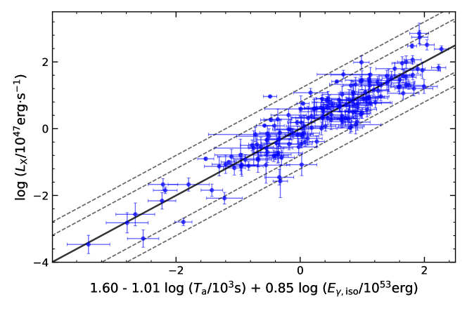
(a)

Figure 1: The best-fit result of the L-T-E correlation with the 174 GRBs taken from Tang et al. (2019). The solid line represents the best result and the dash lines represent $2\sigma$ and $3\sigma$ confidence levels.

3 Standardizing GRBs using SNe Ia

In Section 2, we derived the L-T-E correlation by assuming fixed values for some cosmology parameters such as $H_{0}$, $\Omega_{m}$, $\Omega_{\Lambda}$, and $w$. However, in order to use this GRB sample to study the Universe, we first need to derive a L-T-E correlation that is independent of the cosmological models. Here we choose the same method as presented by Liang et al. (2008), i.e., calibrating GRBs with SNe Ia. There are two main steps in the process: 1) use an available sample of SNe Ia to calibrate the distance modulus ($\mu$) of the low-redshift GRBs and get the best-fit coefficients of the L-T-E correlation with the calibrated low-redshift GRBs; 2) use the fitting results and L-T-E correlation to calculate the model-independent $\mu^{\prime}$ of the high-redshift GRBs and get some constraints on cosmological parameters.

We use the so-called “Pantheon sample” of SNe Ia (Scolnic et al., 2018) to calibrate low-redshift GRBs. This sample includes 1048 SNe Ia, of which the maximum redshift is 2.26. However, except for one event with a redshift of 2.26, all other SNe Ia have a redshift less than 2.0. As a result, the “Pantheon sample” actually is effective in calibrating our GRBs only in the region of $z<2.0$. Considering this ingredient, we divide our GRB sample into two sub-samples according to the distance, a low-redshift sample with 85 GRBs ($z<2$) and a high-redshift sample with 89 GRBs ($z>2$). The boundary is $z=2.0$.

3.1 Redshift evolution of the L-T-E correlation

In order to be a satisfactory standard candle, the correlation itself should not evolve at different redshifts. In this case, we can then safely apply the derived correlation, calibrated at low redshifts, to high redshifts to constrain cosmological parameters. If the correlation does evolve at different redshifts, then it could still be used only when the evolution property is thoroughly known so that its effect can be compensated. Otherwise, it cannot be used as a standard candle.

To test whether the L-T-E correlation evolves with redshift, we can re-fit the three parameter equation by using the two sub-groups, i.e. the low-redshift one and the high-redshift one. To check it in more details, we have further grouped the GRBs into four redshift bins, i.e., $z<1,1<z<2,2<z<3,3<z$. There are about 40 GRBs in each bin. For these various sub-samples, the best-fit L-T-E correlations are presented in Table 3.1.

Table 1: Redshift evolution test of the $L_{x}-T_{a}-E_{\gamma,\rm{iso}}$ correlation.

Redshift range	$a$	$b$	$c$	$\sigma_{\rm{ext}}$	GRB number
Full data	1.60 $\pm$ 0.06	-1.01 $\pm$ 0.05	0.85 $\pm$ 0.04	0.40 $\pm$ 0.03	174
$z<2$	1.45 $\pm$ 0.11	-0.94 $\pm$ 0.08	0.84 $\pm$ 0.06	0.43 $\pm$ 0.04	85
$z>2$	1.51 $\pm$ 0.08	-0.98 $\pm$ 0.07	0.56 $\pm$ 0.09	0.31 $\pm$ 0.04	89
$z<1$	1.28 $\pm$ 0.20	-0.97 $\pm$ 0.13	0.80 $\pm$ 0.09	0.52 $\pm$ 0.07	44
$1<z<2$	1.32 $\pm$ 0.14	-0.84 $\pm$ 0.09	0.65 $\pm$ 0.11	0.31 $\pm$ 0.05	41
$2<z<3$	1.63 $\pm$ 0.12	-1.07 $\pm$ 0.12	0.70 $\pm$ 0.14	0.29 $\pm$ 0.05	42
$3<z$	1.37 $\pm$ 0.10	-0.84 $\pm$ 0.10	0.34 $\pm$ 0.13	0.32 $\pm$ 0.05	47

Table 3.1 indicates that the L-T-E correlation indeed evolves with redshift. This can be most clearly seen from the coefficient “$c$”, which links the X-ray luminosity and the isotropic energy. For the $z<2$ sub-sample, $c=0.84\pm 0.06$, but it changes to $0.56\pm 0.09$ when $z>2$. As for $a$ and $b$, their variation can almost be ignored within the error bars. Anyway, the variation of a single coefficient indicates that the whole L-T-E correlation evolves with redshift. To make it more intuitive, using the best-fit L-T-E equation derived from the high-redshift sub-sample, we plot all the low-redshift and high-redshift GRBs in Figure 2. We see that while the high-redshift GRBs distribute normally along the best-fit line, there is a systematic deviation for the low-redshift events. When the GRBs are grouped into four redshift bins, the evolution of the best-fit L-T-E correlation can also be clearly seen. The coefficient $c$ obviously decreases with the increase of the redshift. It varies from $0.80\pm 0.09$ for $z<1$ to $0.34\pm 0.13$ for $z>3$. In Figure 3, we have plotted the best-fit coefficients of $a,b,c$ versus the redshift bins, which shows the decreasing tendency of $c$ directly.

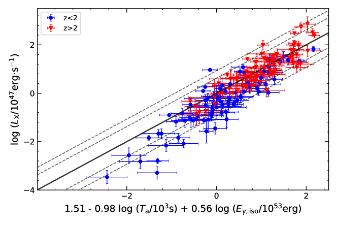
(a)

Figure 2: The best-fit L-T-E correlation of the high-redshift ($z>2$) GRB sub-sample (triangle points). As a comparison, the low-redshift ($z<2$) GRBs are also plotted (dotted points). The high-redshift GRBs distribute normally along the best-fit line, while the low-redshift events systematically deviate from the line. The dashed lines represent $2\sigma$ and $3\sigma$ confidence levels.

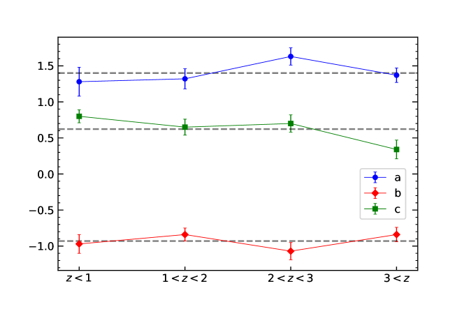
(a)

Figure 3: The variation of the best-fit coefficients among different redshift bins. The dash lines represent the average values of the best-fit coefficients.

3.2 Cosmology from the L-T-E correlation

The redshift evolution indicates that the L-T-E correlation cannot act as a satisfactory standard candle. One may not expect encouraging results on the cosmological parameters by using this correlation. Anyway, assuming that the L-T-E correlation could be used, we continue our calculations to see how the results would be.

As the first step, we need to standardize GRBs and obtain a credible L-T-E correlation equation. We use a linear interpolation method to get the distance modulus ($\mu$) of the low-redshift GRBs, i.e.,

$$\mu_{\rm{GRB}}=\frac{z_{i+1}-z}{z_{i+1}-z_{i}}\mu_{i}+\frac{z-z_{i}}{z_{i+1}-z_{i}}\mu_{i+1},$$ (11)

where $\mu_{\rm{GRB}}$ represents the derived distance modulus of a low-redshift GRB at $z$, while $\mu_{i+1}$ and $\mu_{i}$ are the distance modulus of observed SNe Ia at the nearby redshifts $z_{i+1}$ and $z_{i}$, respectively. Using the corresponding error bars of nearby SNe Ia, namely $\epsilon_{\mu,i+1}$ and $\epsilon_{\mu,i}$, the error bar of the GRB distance modulus ($\sigma_{\mu}$) can be calculated from

$$\sigma_{\mu}^{2}=\left(\frac{z_{i+1}-z}{z_{i+1}-z_{i}}\right)^{2}\epsilon_{\mu,i}^{2}+\left(\frac{z-z_{i}}{z_{i+1}-z_{i}}\right)^{2}\epsilon_{\mu,i+1}^{2}.$$ (12)

After obtaining the distance modulus, we can get the luminosity distance from

$$\mu=5\log\frac{d_{\rm{L}}}{\rm{Mpc}}+25=5\log\frac{d_{\rm{L}}}{\rm{cm}}-97.45.$$ (13)

Using this calibrated luminosity distance, we then go further to re-calculate $L_{X}$ and $E_{\gamma,\rm{iso}}$ of the low-redshift GRBs by using Equations (6) and (8). At this stage, we have the three key parameters ($L_{X},T_{a}$, and $E_{\gamma,\rm{iso}}$) of all low-redshift GRBs at hand and are ready to re-derive a calibrated L-T-E correlation. Again, we use the MCMC method to get the best-fit result, which gives the coefficients as $a=1.41\pm 0.11$, $b=-0.93\pm 0.08$, $c=0.83\pm 0.06$, with an extrinsic scatter of $\sigma_{\rm{ext}}=0.41\pm 0.04$. This calibrated correlation is independent of any cosmological models and should be more reliable.

By directly extrapolating the calibrated L-T-E correlation to high-redshift GRBs, we can get their model-independent $\mu^{\prime}$ through Equations (6),(8),(9), and (13), i.e.,

$$\mu^{\prime}=\frac{5}{2(1-c)}\left[a+b\log T_{a}+c\log\frac{4\pi S}{(1+z)^{3-\alpha_{\gamma}}}-\log\frac{4\pi F_{X0}2^{-1/\omega}}{(1+z)^{2-\beta_{X}}}\right]-97.45,$$ (14)

where $S$ is in units of erg cm^-2 and $F_{X0}$ is in units of erg cm^-2 s^-1. Correspondingly, the error bar of $\mu^{\prime}$ can also be calculated by taking the extrinsic scatter $\sigma_{\rm{ext}}$ into account,

$$\sigma_{\mu^{\prime}}=\frac{5}{2(1-c)}\Bigg{\{}\sigma_{\rm{ext}}^{2}+\sigma_{a}^{2}+\sigma_{b}^{2}\log^{2}T_{a}+b^{2}\sigma^{2}_{\log T_{a}}+(\frac{\sigma_{F_{X0}}}{\ln 10\ F_{X0}})^{2}+\log^{2}2\ (\frac{\sigma_{\omega}}{\omega^{2}})^{2}+\sigma_{\beta_{X}}^{2}\log^{2}(1+z)$$ (15)

$$+(\frac{\sigma_{c}}{1-c})^{2}\left[a+b\log T_{a}-\log\frac{F_{X0}2^{-1/\omega}}{(1+z)^{2-\beta_{X}}}\right]^{2}+(\frac{\sigma_{c}}{1-c})^{2}\log^{2}\frac{S}{(1+z)^{3-\alpha_{\gamma}}}+c^{2}\left[(\frac{\sigma_{S}}{\ln 10\ S})^{2}+\sigma_{\alpha_{\gamma}}^{2}\log^{2}(1+z)\right]\Bigg{\}}^{1/2}.$$

In order to get the best-fit cosmological parameters, we maximize the likelihood function, $\mathcal{L}_{\rm{GRB}}(\theta)$, which is constructed as (Amati et al., 2019)

$$\mathcal{L}_{\rm{GRB}}(\theta)=\prod_{i=1}^{\mathcal{N}_{\rm{GRB}}}\frac{1}{\sqrt{2\pi}\sigma(z_{i})}\exp\left[-\frac{1}{2}\left(\frac{\mu^{\prime}(z_{i})-\mu_{\rm{th}}(z_{i},\theta)}{\sigma(z_{i})}\right)^{2}\right],$$ (16)

where $\theta$ represents a set of cosmological parameters and $\mu_{\rm{th}}$ can be derived from Equations (3) and (13). $\mathcal{N}_{\rm{GRB}}$ here is the number of the high-redshift GRBs.

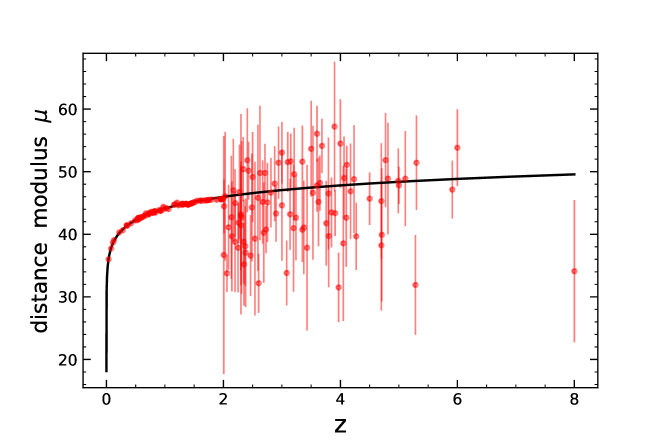
(a)

Figure 4: Calibrated GRB Hubble diagram using the L-T-E correlation. The data points represent our GRB sample. As a comparison, the solid curve corresponds to the theoretical distance modules calculated for a flat $\Lambda$CDM model with $H_{0}=70.0$ km s^-1 Mpc^-1 and $\Omega_{m}=0.289$.

Following the procedure described above, we have taken a test to see whether the L-T-E correlation can be used to constrain the cosmological parameters or not. The Hubble diagram derived from our GRB sample is plotted in Figure 4. At low redshift of $z<2$, we use the SNe Ia sample to calibrate the L-T-E correlation. The calibrated correlation is then extended to high-redshift regime of $z>2$. We see that the high-redshift data points are highly dispersive with large error bars, which means they can hardly give any meaningful constraints on the cosmological parameters. There are at least two reasons for the fact that the L-T-E correlation fails to be a satisfactory cosmological probe. First, the L-T-E correlation is subjected to an obvious redshift evolution as described in the above subsection. As a result, it is inappropriate to extrapolate the calibrated low-redshift relation to high-redshift GRBs directly. Second, and more importantly, both $L_{X}$ and $E_{\gamma,\rm{iso}}$ are proportional to the square of the luminosity distance, which itself is dependent on cosmological parameters. At the same time, the best-fit value of the coefficient $c$ is close to 1. It means the cosmological effect is largely canceled out in the L-T-E correlation, so that the correlation is insensitive to cosmological parameters.

4 The L-T-E_p correlation

The L-T-E correlation is not a good probe for cosmology. Here we explore the possibility of finding another appropriate pattern. Noticing that the spectral peak energy $E_{\rm{p}}$ is closely correlated with $E_{\gamma,\rm{iso}}$ (Amati et al., 2002), we conjecture that there may exist a correlation among $L_{X}$, $T_{a}$, and $E_{\rm{p}}$. We write the potential relation as

$$\log{\frac{L_{X}}{10^{47}\rm{erg/s}}}=a^{\prime}+b^{\prime}\log{\frac{T_{a}}{10^{3}\rm{s}}}+c^{\prime}\log{\frac{E_{\rm{p}}}{\rm{keV}}},$$ (17)

where $E_{\rm{p}}=E_{\rm{p,obs}}\times(1+z)$ and $E_{\rm{p,obs}}$ is the observed peak energy in the $\nu F_{\nu}$ spectrum. We now go on to derive the best-fit coefficients and assess the compactness of this relation. Note that the correlation among $L_{X}$, $T_{a}$, and $E_{\rm{p}}$ has been explored by Izzo et al. (2015). In their studies, they have further included a fourth parameter of $\alpha$ (the timing index of the power-law decaying phase that follows the plateau segment) to get the so-called Combo-relation as $L_{X}\propto(T_{a}/|1+\alpha|)^{-1}E_{\rm{p}}^{0.84\pm 0.08}$ (Izzo et al., 2015; Muccino et al., 2021). It can be regarded as a four-parameter relation. In calibrating the relation, they have used a technique that does not require a large sample of SNe Ia, thus it is less dependent on other cosmological rulers (Izzo et al., 2015). Additionally, the Combo-relation is found to have no redshift evolution (Muccino et al., 2021). As a result, the relation has been effectively used to constrain cosmological parameters (Izzo et al., 2015; Muccino et al., 2021).

Meanwhile, it is interesting to find that the fundamental plane relation, i.e. the $L_{X}-T_{a}-L_{\rm{p}}$ correlation, is only one parameter different from the L-T-E_p correlation. This relation was first established by Dainotti et al. (2016) with a total sample of 176 Swift GRBs. Also, they found the scatter of this relation became smaller when using a class-specific GRB sample. Recently, in Dainotti et al. (2020), they applied new criteria for GRB data sample, and obtained the so-called “Platinum Sample”. With this sample, they performed the Efron & Petrosian method (Efron & Petrosian, 1992) to remove the possible evolution in these three parameters and tried to find the intrinsic relation between these three parameters. Finally, a tight relationship between these three parameters was derived as $L_{X}\propto T_{a}^{-0.86\pm 0.13}L_{\rm{p}}^{0.56\pm 0.12}$ with a small extrinsic scatter of about 0.22.

4.1 Sample selection and the L-T-E_p data

Our new sample consist of the GRBs as investigated by Tang et al. (2019). We select all the events with the $E_{\rm{p}}$ values available. For the parameter of $E_{\rm{p}}$, we collect the data from the following sources:

• Several papers involving the $E_{\rm{p}}-E_{\gamma,\rm{iso}}$ correlation investigation (Demianski et al., 2017; Minaev & Pozanenko, 2020);

• The GRB catalogs of GBM/Fermi (Gruber et al., 2014; von Kienlin et al., 2014; Narayana Bhat et al., 2016; von Kienlin et al., 2020) and Swift (Lien et al., 2016);

• The GCN circulars archive;

• A useful GRB database composed by Wang et al. (2020).

It should be noted that we omit all the short GRBs (7 events) included in Tang et al. (2019), because the $E_{\rm{p}}-E_{\gamma,\rm{iso}}$ correlation is different for short and long GRBs (Demianski et al., 2017). Also, several GRBs have been dropped out due to their poorly constrained $E_{\rm{p}}$. Finally we obtained a sample with 121 long GRBs. The details of this sample are listed in Table 2.

4.2 L-T-E_p correlation

With the new data set, we now examine if there is a correlation among $L_{X}$, $T_{a}$, and $E_{\rm{p}}$. We use the same MCMC method as described in the above section. When all the events are engaged as a whole, we find that the best-fit result is $a^{\prime}=-1.03\pm 0.37$, $b^{\prime}=-1.08\pm 0.08$, $c^{\prime}=0.76\pm 0.14$, with an extrinsic scatter of $\sigma_{\rm{ext}}=0.54\pm 0.04$. The fitting result is illustrated in Figure 5. We see that there does exist an obvious correlation among the three parameters, i.e., $L_{X}\propto T_{a}^{-1.08\pm 0.08}E_{\rm{p}}^{0.76\pm 0.14}$. We call this correlation the L-T-E_p correlation. Comparing with the Combo-relation of $L_{X}\propto(T_{a}/|1+\alpha|)^{-1}E_{p}^{0.84\pm 0.08}$ (Izzo et al., 2015; Muccino et al., 2021), we notice that the power-law indices of both $E_{p}$ and $T_{a}$ are interestingly consistent with each other in the two expressions.

Whether the new L-T-E_p correlation evolves with redshift should also be examined. For this purpose, we divide the sample into two sub-samples, the high-redshift sub-sample ($z>2$) and the low-redshift sub-sample ($z<2$). We have re-fit the L-T-E_p correlation upon each sub-sample. The results are shown in Table 3. We see that the preferred value of $a$ is $-1.01$ when $z<2$, but it is 0.06 when $z>2$. Also, the preferred value of $c$ varies from 0.62 ($z<2$) to 0.44 ($z>2$). It indicates that the L-T-E_p correlation also suffers from the redshift evolution. This is somewhat unexpected, and is different from the Combo-relation which is almost redshift-independent (Muccino et al., 2021).

4.3 De-evolved L-T-E_p correlation

Three quantities ($L_{X}$, $T_{a}$, and $E_{\rm{p}}$) are involved in the L-T-E_p correlation. Each quantity itself could be redshift dependent (Dainotti et al., 2013b) and the redshift evolution of the whole relation thus might be a joint effect of the three quantities (Demianski et al., 2017). To compensate for the redshift evolution, a natural idea is to assume that each quantity depends on the redshift as a power-law function of $(1+z)$ with a certain index (Dainotti et al., 2013b). However, since the L-T-E_p correlation itself is a simple power-law function ($L_{X}\propto T_{a}^{b^{\prime}}E_{\rm{p}}^{c^{\prime}}$), we can also add a single power-law term of $(1+z)^{d^{\prime}}$ into the correlation function to synthesize the overall evolution effects of the three quantities (Demianski et al., 2017), i.e., the possible redshift evolution of individual variable ($L_{X}$, $T_{a}$, and $E_{\rm{p}}$) is synthesized in the new parameter of $d^{\prime}$. Here we choose the simple power-law parameterization to simplify the calculation, different parameterization can be applied to flatten the function at higher redshifts (Singal et al., 2011; Dainotti et al., 2015; Petrosian et al., 2015). In this case, we re-write the L-T-E_p correlation as

$$\log{\frac{L_{X}}{10^{47}\rm{erg/s}}}=a^{\prime}+b^{\prime}\log{\frac{T_{a}}{10^{3}\rm{s}}}+c^{\prime}\log{\frac{E_{\rm{p}}}{\rm{keV}}}+d^{\prime}\log(1+z).$$ (18)

We use this new function to re-fit our data set. The result is also presented in Table 3. It is found that the best-fit coefficient is $d^{\prime}=1.78\pm 0.29$, which is significantly larger than 1. It indicates there really is a significant redshift evolution in the direct L-T-E_p correlation. As a comparison, we have also done a similar test for the L-T-E correlation of Section 3. The best-fit parameter of $d^{\prime}$ is only $d^{\prime}=1.04\pm 0.25$. It means that the redshift evolution of the L-T-E_p correlation, if not corrected for, is even more significant than that of the previous L-T-E correlation.

To rectify the evolution effect, we remove the redshift dependent term in Equation 18 and replace $L_{X}$ with a calibrated X-ray luminosity of

$$L_{X,\rm{cal}}=\frac{L_{X}}{(1+z)^{d^{\prime}}}.$$ (19)

The calibrated data of the X-ray luminosity are also listed in Table 2 and the de-evolved L-T-E_p correlation can be written as

$$\log{\frac{L_{X,\rm{cal}}}{10^{47}\rm{erg/s}}}=a^{\prime\prime}+b^{\prime\prime}\log{\frac{T_{a}}{10^{3}\rm{s}}}+c^{\prime\prime}\log{\frac{E_{\rm{p}}}{\rm{keV}}}.$$ (20)

Using this equation, the best-fit results for both low-redshift and high-redshift GRBs are shown in Table 3. Now, the derived coefficients are almost identical for both sub-samples, which means no further redshift evolution exists. In Figure 5, we have plotted the best-fit results of the de-evolved L-T-E_p correlation upon the full sample. Comparing with the direct L-T-E_p correlation, the de-evolved L-T-E_p correlation is more tighten and the data points of both the low-redshift and high-redshift sub-samples are distributed normally along the best-fit line.

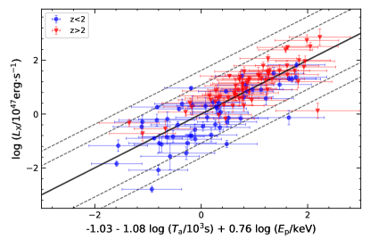
(a)

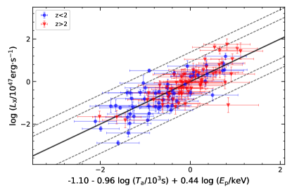
(b)

Figure 5: The best-fit result of the L-T-E_p correlation (left panel) and the de-evolved L-T-E_p correlation (right panel). In the left panel, there is a clear systematic deviation between the low-redshift sub-sample and the high-redshift sub-sample. In the right panel, both sub-samples distributed normally along the best-fit line.

We have further checked the possible evolution of each parameter. For this purpose, we perform the Efron & Petrosian method (Efron & Petrosian, 1992) to get the redshift evolution of $L_{X}$, $T_{a}$, and $E_{\rm{p}}$ separately (details of this method are presented in the Appendix). We take a simple power-law function $(1+z)^{k}$ as the evolution form of each parameter. Now we have three power-law indices, $k_{L_{X}}$, $k_{T_{a}}$, and $k_{E_{\rm{p}}}$ for $L_{X}$, $T_{a}$, and $E_{\rm{p}}$, respectively. Our analyses show that all the three parameters evolve with redshift (see the Appendix for details). For $L_{X}$ and $T_{a}$, we get $k_{L_{X}}=3.38\pm 0.62$ and $k_{T_{a}}=-1.54\pm 0.30$. These two indices are somewhat different from those derived by Dainotti et al. (2017b), in which both $L_{X}$ and $T_{a}$ have a smaller evolution ($k_{L_{X}}=-0.40_{-0.83}^{+0.89}$ and $k_{T_{a}}=-0.17_{-0.37}^{+0.41}$). The difference may be due to the fact that different samples are used in the two studies. Also, note that the error bars derived in both studies are still quite large, further studies on this aspect are necessary when more data are available in the future. As for $k_{E_{\rm{p}}}$, we get $k_{E_{\rm{p}}}=0.75\pm 0.25$, which also shows a significant redshift evolution.

After correcting for the redshift evolution of each parameter, we can also get a new separate de-evolved L-T-E_p correlation as

$$\log{\frac{L_{X}/(1+z)^{k_{L_{X}}}}{10^{47}\rm{erg/s}}}=a^{\prime\prime\prime}+b^{\prime\prime\prime}\log{\frac{T_{a}/(1+z)^{k_{T_{a}}}}{10^{3}\rm{s}}}+c^{\prime\prime\prime}\log{\frac{E_{\rm{p}}/(1+z)^{k_{E_{\rm{p}}}}}{\rm{keV}}}.$$ (21)

Using the MCMC method, we get the best-fit coefficients for this correlation as $a^{\prime\prime\prime}=-0.88\pm 0.36$, $b^{\prime\prime\prime}=-0.87\pm 0.10$, $c^{\prime\prime\prime}=0.35\pm 0.16$, and $\sigma=0.44\pm 0.05$. The extrinsic scatter is smaller compared with the direct L-T-E correlation, which indicates that this new correlation does have made compensation for the redshift evolution to some extent.

5 Cosmology with de-evolved L-T-E_p correlation

In this section we use the de-evolved L-T-E_p correlation to constrain the cosmological parameters. It is well known that there is a problem called “the Hubble tension”, which means even the Hubble constant is not well determined. For example, the Hubble constant derived from Planck Collaboration et al. (2020) was $H_{0}=67.4\pm 0.5$ km s^-1 Mpc^-1, while Riess et al. (2019) used the distance-ladder measurements of LMC Cepheids and got $H_{0}=74.03\pm 1.42$ km s^-1 Mpc^-1. In our study, we fix this parameter as $H_{0}=70.0$ km s^-1 Mpc^-1 for simplicity. First, using the same method as described in Section 3.2, we do a linear interpolation with the help of the SNe Ia sample to get the calibrated $\mu$ of the low-redshift GRBs. From the low-redshift GRBs, the best-fit result of the de-evolved L-T-E_p correlation corresponds to $a^{\prime\prime}=-1.34\pm 0.50$, $b^{\prime\prime}=-0.89\pm 0.11$, $c^{\prime\prime}=0.50\pm 0.20$ and $\sigma_{\rm{ext}}=0.52\pm 0.07$. Thus, the de-evolved L-T-E_p correlation can be written as

$$L_{X,\rm{cal}}\propto T_{a}^{-0.89\pm 0.11}E_{\rm{p}}^{0.50\pm 0.20}.$$ (22)

Because this de-evolved L-T-E_p correlation does not evolve with redshift, it is applicable for the high-redshift sample.

The $L_{X}$ values of the high-redshift GRBs can be derived from Equations (19) and (20). The propagated uncertainties of $L_{X}$ can be calculated from

$$\sigma_{\log L_{X}}^{2}=\sigma_{a^{\prime\prime}}^{2}+\sigma_{b^{\prime\prime}}^{2}\log^{2}T_{a}+b^{\prime\prime 2}\sigma^{2}_{\log T_{a}}+\sigma_{c^{\prime\prime}}^{2}\log^{2}E_{\rm{p}}+c^{\prime\prime 2}\sigma^{2}_{\log E_{\rm{p}}}+\sigma_{d^{\prime}}^{2}\log^{2}(1+z)+\sigma_{\rm{ext}}^{2}.$$ (23)

The model-independent $\mu^{\prime}$ is calculated through Equations (6), (13), and (19). The final uncertainty of the distance modulus is given by

$$\sigma_{\mu^{\prime}}=\frac{5}{2}\left[\sigma_{\log L_{X}}^{2}+(\frac{\sigma_{F_{X0}}}{\ln 10\ F_{X0}})^{2}+\log^{2}2\ (\frac{\sigma_{\omega}}{\omega^{2}})^{2}+\sigma_{\beta_{X}}^{2}\log^{2}(1+z)\right]^{1/2}.$$ (24)

In Figure 6, we present the Hubble diagram as built by using the calibrated distance modulus. With the model-independent $\mu^{\prime}$ of the high-redshift GRBs, we can get some constraints on the cosmological parameters by using Equation (16). At the same time, we should also note that the error bars of the derived distance modulus of the high-redshift GRBs are still a bit too large, it means the cosmological parameters cannot be accurately measured by simply using the devolved L-T-E_p correlation alone currently. It can only be used as a supplementary tool.

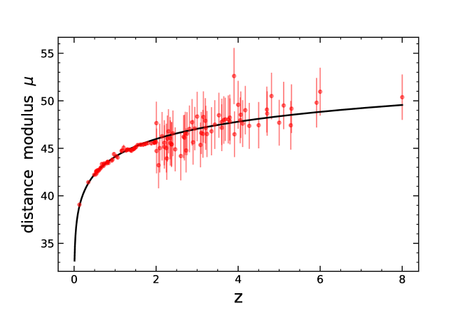
Figure 6: Calibrated GRB Hubble diagram from the de-evolved L-T-E_p correlation. The data points correspond to our GRB sample. As a comparison, the black line is the theoretical distance modulus calculated for the flat $\Lambda$CDM model with $H_{0}=70.0$ km s^-1 Mpc^-1 and $\Omega_{m}=0.289$.

Anyway, as the first step, we have made a test to see what constraints can be derived by using only the GRBs. In this case, for the flat $\Lambda$CDM model, we obtain $\Omega_{m}=0.389^{+0.202}_{-0.141}$. When considering a non-flat $\Lambda$CDM model, the best-fit result gives $\Omega_{m}=0.333^{+0.188}_{-0.142}$ and $\Omega_{\Lambda}=0.346^{+0.356}_{-0.249}$. Furthermore, if the flat $w$CDM model is considered, where $w$ describes the dark energy equation of state (EOS), then we get $\Omega_{m}=0.369^{+0.217}_{-0.191}$ and $w=-0.966^{+0.513}_{-0.678}$. Note that the EOS parameter ($w$) is very close to the standard value of $-1$. However, in all these results, the uncertainties of the derived parameters are large. The results are summarized in Table 4.

As mentioned before, the circularity problem is a key issue that should be paid special attention to when using various standard candles to measure the Universe. For the de-evolved L-T-E_p correlation, an interesting method that can help overcome the difficulty is to simultaneously derive the coefficients of the relation and the cosmological parameters by fitting the observational data. In this case, no cosmological models would be assumed in the first place and this simultaneous fitting method does not suffer from the circularity problem. In our study, we have also tried this method to further check our results.

Following Dainotti et al. (2013a), the likelihood function will be similar to Equation (10) and we only need to add extra cosmological parameters into the parameter space. For the sake of a direct comparison, here we still use the D’Agostini’s likelihood (D’Agostini, 2005), but not the Reichart’s likelihood (Reichart, 2001). The likelihood function now becomes

$$\mathcal{L}(a,b,c,\sigma_{\rm{ext}},p_{c})\propto\prod_{i}\frac{1}{\sqrt{\sigma_{\rm{ext}}^{2}+(\sigma_{L_{X}}^{i})^{2}+b^{2}(\sigma_{T_{a}}^{i})^{2}+c^{2}(\sigma_{E_{\rm{p}}}^{i})^{2}}}$$ (25)

$$\times\exp\left[-\frac{\left(L_{X}^{i}(p_{c})-a-bT_{a}^{i}-cE_{\rm{p}}^{i}\right)^{2}}{2\left(\sigma_{\rm{ext}}^{2}+(\sigma_{L_{X}}^{i})^{2}+b^{2}(\sigma_{T_{a}}^{i})^{2}+c^{2}(\sigma_{E_{\rm{p}}}^{i})^{2}\right)}\right],$$

where $p_{c}$ refers to a set of cosmological parameters. Here the cosmological parameters are free and need to be determined together with the correlation coefficients.

Using this likelihood function, we have re-fitted the observed plateau data. For a non-flat $\Lambda$CDM model, our best-fit results are illustrated in Figure 7. We find that the de-evolved L-T-E_p correlation now becomes $L_{X,\rm{cal}}\propto T_{a}^{-0.95\pm 0.07}E_{\rm{p}}^{0.43\pm 0.13}$. This expression is well consistent with the above result of Equation (22). Correspondingly, the derived cosmological parameters are $\Omega_{m}=0.50^{+0.30}_{-0.26}$ and $\Omega_{\Lambda}=0.23^{+0.29}_{-0.17}$. It is also consistent with the results presented above. Similarly, for a flat universe, by using the simultaneous fitting method, we get the cosmological parameters as $\Omega_{m}=0.62^{+0.26}_{-0.35}$ and $w=-0.65^{+0.47}_{-0.86}$ for the $w$CDM model, and $\Omega_{m}=0.71^{+0.20}_{-0.28}$ for the $\Lambda$CDM model. We also plot the best-fit results for the flat $\Lambda$CDM model in Figure 8. These results are all consistent with the above results within $1\sigma$ confidence level, but with a larger uncertainty. It clearly shows that our previous calibration and de-evolution processes are credible. We will continue to use our previous calibration method in the following study for simplicity and clarity.

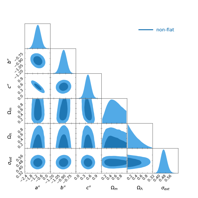
Figure 7: De-evolved L-T-E_p correlation coefficients and cosmological parameters derived by using the simultaneous fitting method, which is not subjected to the so-called circularity problem. This figure is plotted for a non-flat $\Lambda$CDM model (68% and 95% confidence levels are shown). The best-fit correlation coefficients are $a^{\prime\prime}=-1.19\pm 0.33$, $b^{\prime\prime}=-0.95\pm 0.07$, $c^{\prime\prime}=0.43\pm 0.13$, and $\sigma_{\rm{ext}}=0.45\pm 0.04$. For the cosmological parameters, we have $\Omega_{m}=0.50^{+0.30}_{-0.26}$, $\Omega_{\Lambda}=0.23^{+0.29}_{-0.17}$. Here the error bars correspond to $1\sigma$ range.

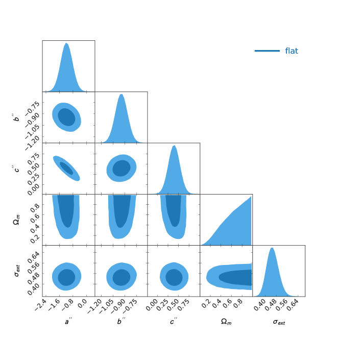
Figure 8: De-evolved L-T-E_p correlation coefficients and cosmological parameters derived by simultaneously fitting the correlation coefficients and the cosmological parameters. Note that this figure is different from Figure 7. It is plotted for a flat $\Lambda$CDM model (68% and 95% confidence levels are shown). The best-fit correlation coefficients are $a^{\prime\prime}=-1.18\pm 0.32$, $b^{\prime\prime}=-0.95\pm 0.07$, $c^{\prime\prime}=0.40\pm 0.13$, and $\sigma_{\rm{ext}}=0.45\pm 0.04$, while the best-fit result for the cosmological parameter is $\Omega_{m}=0.71^{+0.20}_{-0.28}$. Here the error bars correspond to $1\sigma$ range.

With the separate de-evolved L-T-E_p correlation (Equation 21), we have also attempted to use the simultaneous fitting method to constrain cosmological parameters. For the flat $\Lambda$CDM model, the best-fit results are illustrated in Figure 9. We see that the matter density is derived as $\Omega_{m}=0.76_{-0.26}^{+0.17}$. This result is consistent with the former result using the de-evolved L-T-E_p correlation within $1\sigma$ confidence level. Below, we will continue our study in our former framework with the de-evolved L-T-E_p correlation (using SNe Ia calibration) for simplicity.

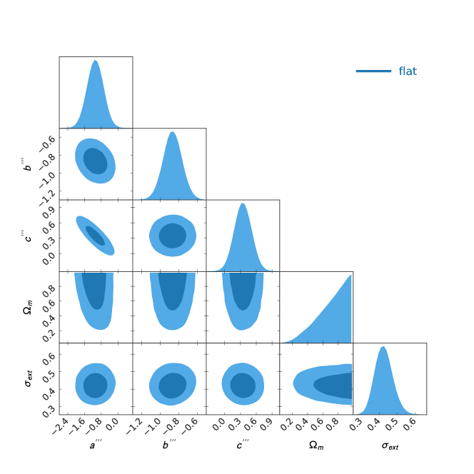
Figure 9: Best-fit correlation coefficients and cosmological parameters derived by using the simultaneous fitting method and the separate de-evolved L-T-E_p correlation (Equation 21). A flat $\Lambda$CDM model is assumed. 68% and 95% confidence levels are shown in the plot. The best-fit correlation coefficients are $a^{\prime\prime\prime}=-1.09\pm 0.35$, $b^{\prime\prime\prime}=-0.86\pm 0.10$, $c^{\prime\prime\prime}=0.35\pm 0.15$, and $\sigma_{\rm{ext}}=0.42\pm 0.04$. The cosmological parameter is derived as $\Omega_{m}=0.76_{-0.26}^{+0.17}$.

Next we combine the devolved L-T-E_p correlation with other cosmological probes, including SNe Ia, CMB, and BAO, to give more stringent constraints on the cosmological parameters. For this purpose, we should effectively synthesize the likelihood functions of various probes.

The likelihood function of SNe Ia is calculated as

$$\mathcal{L}_{\rm{SN}}(\theta)=\prod_{i=1}^{\mathcal{N}_{\rm{SN}}}\frac{1}{\sqrt{2\pi}\sigma_{\rm{SN}}(z_{i})}\exp\left[-\frac{1}{2}\left(\frac{\mu_{\rm{SN}}(z_{i})-\mu_{\rm{th}}(z_{i},\theta)}{\sigma_{\rm{SN}}(z_{i})}\right)^{2}\right],$$ (26)

where $\mu_{\rm{SN}}$ and $\sigma_{\rm{SN}}(z_{i})$ are taken from the Pantheon SNe Ia sample (Scolnic et al., 2018).

For the CMB, we consider a shift parameter $\mathcal{R}$, which is defined as (Wang & Mukherjee, 2006)

$$\mathcal{R}=\frac{\sqrt{\Omega_{m}}}{\sqrt{|\Omega_{k}|}}\rm{sinn}\left(\sqrt{|\Omega_{k}|}\int_{0}^{z_{\ast}}\frac{dz}{E(z)}\right),$$ (27)

where $z_{\ast}$ is the last scattering redshift which we take as $z_{\ast}=1089.90\pm 0.23$ (Planck Collaboration et al., 2016). The function sinn($x$) is defined as sinn($x$)=sin($x$) for a closed Universe, sinn($x$)=sinh($x$) for an open Universe, and sinn($x$) = $x$ for a flat Universe. The likelihood function for CMB is then

$$\mathcal{L}_{\rm{CMB}}(\theta)=\frac{1}{\sqrt{2\pi}\sigma_{\mathcal{R}}}\exp\left[-\frac{1}{2}\left(\frac{\mathcal{R}(\theta)-\mathcal{R}_{\rm{obs}}}{\sigma_{\mathcal{R}}}\right)^{2}\right],$$ (28)

where $\mathcal{R}_{\rm{obs}}$ and $\sigma_{\mathcal{R}}$ are constraints obtained from the 2015 Planck data. We take $\mathcal{R}_{\rm{obs}}=1.7474\pm 0.0051$ for a non-flat Universe and $\mathcal{R}_{\rm{obs}}=1.7482\pm 0.0048$ for a flat Universe (Wang & Dai, 2016).

As for the BAO, we use the data provided by Alam et al. (2017) and the likelihood for BAO can be generally calculated as (Sánchez et al., 2017; Tu et al., 2019)

$$\mathcal{L}_{\rm{BAO}}(\theta)\propto\frac{1}{\sqrt{2\pi}}\exp\left[-\frac{1}{2}(V_{\rm{obs}}-V_{\rm{th}})C^{-1}(V_{\rm{obs}}-V_{\rm{th}})^{T}\right],$$ (29)

where the subscripts “obs” and “th” represent observed value and theoretical value respectively. Here $V$ can be either the transverse co-moving distance $D_{M}$ or the Hubble parameter $H_{z}$. $C^{-1}$ is the inverse covariance matrix of the observed variables. We list the covariance matrix and the observational data in Table 5 (Alam et al., 2017). Note that $D_{M}$ in Table 5 can be calculated as $D_{M}=d_{\rm{L}}/(1+z)$, and $H_{z}$ is defined as $H_{z}=H_{0}E(z)$.

To combine all the probes described above, we can define a joint likelihood function as $\mathcal{L}=\mathcal{L}_{\rm{GRB}}\mathcal{L}_{\rm{SN}}\mathcal{L}_{\rm{CMB}}\mathcal{L}_{\rm{BAO}}$.

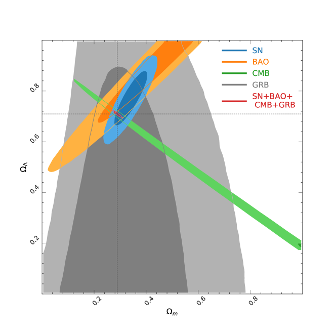
Figure 10: Constraints on $\Omega_{m}-\Omega_{\Lambda}$ for the non-flat $\Lambda$CDM model (68% and 95% confidence levels) with observational data of SNe Ia (blue), BAO (orange), CMB (green) and the de-evolved L-T-E_p correlation of GRBs (grey). The joint constraint from all the four probes is shown as the inner red contours. The dashed lines show the most probable value of $\Omega_{m}$ and $\Omega_{\Lambda}$ derived by using the four probes, i.e., $\Omega_{m}=0.289\pm 0.008$, $\Omega_{\Lambda}=0.710\pm 0.006$

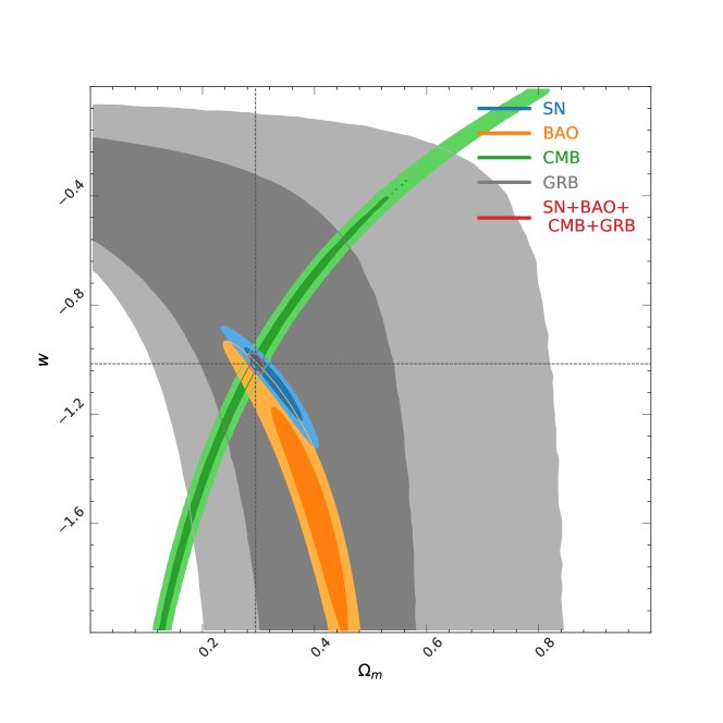
Figure 11: Constraints on $\Omega_{m}-w$ for the flat $w$CDM model (68% and 95% confidence levels) with observational data of SNe Ia (blue), BAO (orange), CMB (green) and the de-evolved L-T-E_p correlation of GRBs (grey). The joint constraint from the four cosmological probes is shown as the inner red contours. The dashed lines show the most probable value of $\Omega_{m}$ and $w$ derived by using the four probes, i.e., $\Omega_{m}=0.295\pm 0.006$ and $w=-1.015\pm 0.015$.

We have used the de-evolved L-T-E_p correlation to constrain the cosmological parameters. When only this probe is engaged, we obtain a result of $\Omega_{m}=0.389^{+0.202}_{-0.141}(1\sigma)$ for the flat $\Lambda$CDM model. We see that the uncertainty is quite large, due to the fact that the correlation is still a bit too dispersive (see Figure 6). However, this result does not conflict with our current understanding of the Universe. It is also consistent with the cosmological results derived from the Combo-relation (Izzo et al., 2015; Muccino et al., 2021). Combined with other probes such as the SNe Ia (Betoule et al., 2014; Scolnic et al., 2018; Abbott et al., 2019), CMB (Planck Collaboration et al., 2016, 2020), and BAO (Alam et al., 2017), we obtain $\Omega_{m}=0.289\pm 0.008$ and $\Omega_{\Lambda}=0.710\pm 0.006$ for the non-flat $\Lambda$CDM model. The result is plotted in Figure 10. Although the L-T-E_p correlation can only play a very limited role in the practice currently, it may provide useful help when the sample size increases significantly and when the correlation is more accurately calibrated in the future.

For the flat $w$CDM model, we have also applied the above method to derive the cosmological parameters. When only the de-evolved L-T-E_p correlation is used, we get $\Omega_{m}=0.369^{+0.217}_{-0.191}$ and $w=-0.966^{+0.513}_{-0.678}(1\sigma)$, where the uncertainties are quite large. By combining all the four probes, the best-fit result is $\Omega_{m}=0.295\pm 0.006$ and $w=-1.015\pm 0.015$. This result is consistent with the cosmological-constant model for dark energy. The fitting results are shown in Figure 11, and a summary of all our cosmology results are listed in Table 4.

6 Discussion and conclusions

According to the L-T-E correlation (Xu & Huang, 2012; Tang et al., 2019; Zhao et al., 2019), the end time of the plateau phase ($T_{a}$) and the corresponding X-ray luminosity at that moment ($L_{X}$) are closely related with the isotropic $\gamma$-ray energy release during the prompt burst phase ($E_{\gamma,\rm{iso}}$). It has been expected that this relation may act as a standard candle to provide useful constraints on cosmological parameters. However, in this study, it is shown that there is a clear redshift evolution in the L-T-E correlation, which makes it not a satisfactory standard candle. Additionally, we notice that while both $L_{X}$ and $E_{\gamma,\rm{iso}}$ are proportional to the luminosity distance, their power-law indices in the correlation function are almost identical. It further means that the L-T-E correlation is very insensitive to cosmological parameters. Considering that $E_{\gamma,\rm{iso}}$ is closely related to the peak spectral energy ($E_{\rm p}$), we went further to build a new three parameter correlation, namely the L-T-E_p correlation, which connects the three parameters of $L_{X}$, $T_{a}$, and $E_{\rm p}$ as $L_{X}\propto T_{a}^{-1.08\pm 0.08}E_{\rm{p}}^{0.76\pm 0.14}$. The new L-T-E_p correlation is derived from a sample of 121 long GRBs with a plateau phase in the X-ray afterglow lightcurve. It is largely consistent with the four-parameter Combo-relation of $L_{X}\propto(T_{a}/|1+\alpha|)^{-1}E_{p}^{0.84\pm 0.08}$ (Izzo et al., 2015; Muccino et al., 2021). Our L-T-E_p correlation also suffers from the redshift evolution, but it can be easily corrected for by dividing $L_{X}$ with $(1+z)^{1.78}$. It is found that the best-fit de-evolved L-T-E_p correlation reads $L_{X,\rm{cal}}\propto T_{a}^{-0.89}E_{\rm{p}}^{0.50}$. As a test, we have tried to combine this correlation with other probes to constrain the cosmological parameters. Although the L-T-E_p correlation can only improve the parameters marginally at current stage, it is expected that encouraging results may be available from this new probe when the sample size increases significantly in the future.

Our results are consistent with the normal vision that both high-redshift Universe and low-redshift Universe follow the same pattern. However, some studies have shown a deviation from the $\Lambda$CDM model when using high-redshift cosmological probes like quasars and GRBs (Lusso et al., 2019; Amati et al., 2019; Risaliti & Lusso, 2019; Demianski et al., 2019; Luongo & Muccino, 2020a, b). We want to point out that this tension may not necessarily lead to new fundamental physics beyond the standard model, but may be related with the redshift evolution in the empirical luminosity relations of GRBs and quasars that are used as the candles, and with the calibration method using SNe Ia. The cosmological results at high redshift will be distorted when a kind of “standard candles” are calibrated with low-redshift sample and then directly extended to high redshift if there exists a redshift evolution in the candles themselves. In our studies, we have tried to compensate the redshift evolution in the L-T-E_p correlation as far as possible.

It should also be mentioned that the de-evolved L-T-E_p correlation derived here is still not a very compact relation. It has a relatively large dispersion of $\sigma_{\rm{ext}}\sim 0.5$. The reason may be due to the fact that the three parameters involved are not measured accurately enough. First, the $E_{\rm{p}}$ of different GRBs are extrapolated from the observational data of different detectors. There may be systematic bias in the parameter. Second, for a slowly broken X-ray lightcurve, the determination of the breaking point, i.e. $T_{a}$, is difficult and may subject to large uncertainties. Thirdly, the X-ray luminosities ($L_{X}$) in our sample have been derived from the XRT/Swift observations. However, we know that XRT has a relatively narrow passband, it may bring in a relatively large uncertainty in $L_{X}$. In the future, we hope the three parameters of $L_{X}$, $T_{a}$, and $E_{\rm{p}}$ can be accurately determined for an even larger sample. Then even the L-T-E_p correlation itself may be able to give an accurate constraint on the cosmology model.

Table 2: The sample of 121 GRBs used for the L-T-E_p study.

GRB Name	$z^{a}$	$\log(L_{X})^{a}$	$\log(L_{X,\rm{cal}})^{b}$	$\log(T_{a})^{a}$	$\log(E_{\rm{p}})^{c}$	Detector	Refsc
		($10^{47}$erg/s)	($10^{47}$erg/s)	($10^{3}$s)	(keV)
GRB 050315	1.949	-0.3 $\pm$ 0.24	-1.13 $\pm$ 0.27	1.53 $\pm$ 0.16	2.07 $\pm$ 0.11	Swift	6
GRB 050319	3.24	0.86 $\pm$ 0.22	-0.26 $\pm$ 0.28	0.53 $\pm$ 0.25	2.47 $\pm$ 0.34	Swift	6
GRB 050401	2.9	1.38 $\pm$ 0.18	0.33 $\pm$ 0.25	0.21 $\pm$ 0.14	2.61 $\pm$ 0.05	Konus-Wind	1
GRB 050416A	0.6535	-0.81 $\pm$ 0.17	-1.2 $\pm$ 0.18	0.2 $\pm$ 0.2	1.4 $\pm$ 0.07	Swift	1
GRB 050505	4.27	1.29 $\pm$ 0.15	0.01 $\pm$ 0.26	0.37 $\pm$ 0.08	2.82 $\pm$ 0.16	Swift	1
GRB 050814	5.3	0.52 $\pm$ 0.35	-0.9 $\pm$ 0.42	0.66 $\pm$ 0.3	2.53 $\pm$ 0.06	Swift	1
GRB 050922C	2.199	1.96 $\pm$ 0.19	1.06 $\pm$ 0.24	-0.92 $\pm$ 0.14	2.62 $\pm$ 0.12	HETE-2	1
GRB 051016B	0.9364	-1.13 $\pm$ 0.29	-1.64 $\pm$ 0.3	0.95 $\pm$ 0.19	1.73 $\pm$ 0.2	Swift	6
GRB 051109A	2.346	1.49 $\pm$ 0.15	0.56 $\pm$ 0.21	-0.19 $\pm$ 0.11	2.76 $\pm$ 0.16	Konus-Wind	1
GRB 060115	3.53	0.33 $\pm$ 0.22	-0.83 $\pm$ 0.29	0.38 $\pm$ 0.19	2.45 $\pm$ 0.05	Swift	1
GRB 060116	4	1.2 $\pm$ 0.22	-0.04 $\pm$ 0.3	-0.66 $\pm$ 0.27	2.81 $\pm$ 0.18	Swift	2
GRB 060206	4.05	1.61 $\pm$ 0.22	0.36 $\pm$ 0.3	-0.49 $\pm$ 0.2	2.6 $\pm$ 0.05	Swift	1
GRB 060210	3.91	1.58 $\pm$ 0.17	0.35 $\pm$ 0.26	0.24 $\pm$ 0.09	2.76 $\pm$ 0.14	Swift	1
GRB 060502A	1.51	0.03 $\pm$ 0.2	-0.69 $\pm$ 0.23	0.49 $\pm$ 0.17	2.51 $\pm$ 0.13	Konus-Wind	1
GRB 060522	5.11	1.75 $\pm$ 0.25	0.35 $\pm$ 0.34	-0.89 $\pm$ 0.26	2.63 $\pm$ 0.08	Swift	1
GRB 060526	3.21	0.27 $\pm$ 0.29	-0.84 $\pm$ 0.35	0.63 $\pm$ 0.21	2.02 $\pm$ 0.09	Swift	1
GRB 060605	3.8	0.9 $\pm$ 0.21	-0.31 $\pm$ 0.29	0.3 $\pm$ 0.12	2.69 $\pm$ 0.22	Swift	1
GRB 060607A	3.082	1.41 $\pm$ 0.02	0.33 $\pm$ 0.18	0.5 $\pm$ 0.01	2.76 $\pm$ 0.15	Swift	1
GRB 060614	0.13	-2.79 $\pm$ 0.11	-2.89 $\pm$ 0.11	1.69 $\pm$ 0.04	2.53 $\pm$ 0.23	Swift	1
GRB 060707	3.43	0.59 $\pm$ 0.39	-0.56 $\pm$ 0.43	0.47 $\pm$ 0.33	2.45 $\pm$ 0.04	Swift	1
GRB 060708	2.3	0.6 $\pm$ 0.19	-0.32 $\pm$ 0.24	0.07 $\pm$ 0.14	2.47 $\pm$ 0.22	Swift	2
GRB 060714	2.71	0.97 $\pm$ 0.13	-0.05 $\pm$ 0.21	-0.01 $\pm$ 0.1	2.37 $\pm$ 0.2	Swift	1
GRB 060729	0.54	-0.9 $\pm$ 0.04	-1.23 $\pm$ 0.07	1.62 $\pm$ 0.02	2.49 $\pm$ 0.1	Swift	2
GRB 060814	0.84	-0.38 $\pm$ 0.17	-0.86 $\pm$ 0.19	0.74 $\pm$ 0.09	2.76 $\pm$ 0.22	Konus-Wind	5
GRB 060906	3.685	0.46 $\pm$ 0.16	-0.73 $\pm$ 0.25	0.43 $\pm$ 0.1	2.32 $\pm$ 0.09	Swift	1
GRB 060908	1.8836	1.37 $\pm$ 0.2	0.55 $\pm$ 0.24	-0.7 $\pm$ 0.21	2.71 $\pm$ 0.09	Swift	1
GRB 061021	0.3463	-1.11 $\pm$ 0.13	-1.34 $\pm$ 0.14	0.61 $\pm$ 0.08	2.85 $\pm$ 0.18	Konus-Wind	1
GRB 061121	1.314	0.9 $\pm$ 0.14	0.26 $\pm$ 0.17	0.22 $\pm$ 0.07	3.15 $\pm$ 0.03	Konus-Wind	1
GRB 061222A	2.088	1.09 $\pm$ 0.33	0.22 $\pm$ 0.36	0.42 $\pm$ 0.19	2.96 $\pm$ 0.04	Konus-Wind	1
GRB 070129	2.3384	0.07 $\pm$ 0.15	-0.86 $\pm$ 0.21	0.84 $\pm$ 0.13	2.16 $\pm$ 0.12	Swift	2
GRB 070208	1.165	-0.59 $\pm$ 0.22	-1.19 $\pm$ 0.24	0.59 $\pm$ 0.23	2.05 $\pm$ 0.01	Swift	2
GRB 070306	1.497	0.19 $\pm$ 0.07	-0.52 $\pm$ 0.14	1.09 $\pm$ 0.04	2.36 $\pm$ 0.08	Swift	6
GRB 070508	0.82	0.92 $\pm$ 0.16	0.46 $\pm$ 0.18	-0.06 $\pm$ 0.24	2.53 $\pm$ 0.01	Swift	1
GRB 070714B	0.92	-0.13 $\pm$ 0.26	-0.64 $\pm$ 0.28	-0.13 $\pm$ 0.22	3.33 $\pm$ 0.24	Swift	5
GRB 071020	2.145	0.58 $\pm$ 0.29	-0.3 $\pm$ 0.33	0.5 $\pm$ 0.2	3.01 $\pm$ 0.05	Konus-Wind	1
GRB 080516	3.2	0.79 $\pm$ 0.22	-0.32 $\pm$ 0.28	-0.02 $\pm$ 0.22	2.51 $\pm$ 0	Swift	2
GRB 080603B	2.69	1.8 $\pm$ 0.19	0.79 $\pm$ 0.25	-0.64 $\pm$ 0.25	2.57 $\pm$ 0.13	Konus-Wind	1
GRB 080605	1.6398	1.51 $\pm$ 0.21	0.76 $\pm$ 0.24	-0.22 $\pm$ 0.13	2.84 $\pm$ 0.02	Konus-Wind	1
GRB 080721	2.602	2.74 $\pm$ 0.2	1.75 $\pm$ 0.26	-0.51 $\pm$ 0.1	3.25 $\pm$ 0.04	Konus-Wind	1
GRB 080810	3.35	2 $\pm$ 0.18	0.86 $\pm$ 0.26	-0.43 $\pm$ 0.12	3.17 $\pm$ 0.05	Swift	1
GRB 080905B	2.374	1.42 $\pm$ 0.15	0.48 $\pm$ 0.22	0 $\pm$ 0.11	2.79 $\pm$ 0.12	Fermi	3
GRB 081007	0.5295	-0.93 $\pm$ 0.21	-1.26 $\pm$ 0.22	0.41 $\pm$ 0.18	1.79 $\pm$ 0.11	Swift	1
GRB 081008	1.9685	0.28 $\pm$ 0.26	-0.57 $\pm$ 0.29	0.48 $\pm$ 0.15	2.42 $\pm$ 0.09	Fermi	4
GRB 081221	2.26	2.38 $\pm$ 0.1	1.47 $\pm$ 0.18	-0.72 $\pm$ 0.07	2.42 $\pm$ 0.01	Konus-Wind	1
GRB 090113	1.7493	1.3 $\pm$ 0.11	0.51 $\pm$ 0.17	-0.71 $\pm$ 0.11	2.59 $\pm$ 0.09	Fermi	3
GRB 090205	4.7	0.87 $\pm$ 0.3	-0.47 $\pm$ 0.37	-0.03 $\pm$ 0.22	2.33 $\pm$ 0.15	Swift	4
GRB 090407	1.4485	-0.84 $\pm$ 0.22	-1.53 $\pm$ 0.25	1.56 $\pm$ 0.15	2.88 $\pm$ 0	Swift	2
GRB 090418A	1.608	1.09 $\pm$ 0.18	0.35 $\pm$ 0.22	-0.07 $\pm$ 0.09	3.2 $\pm$ 0.11	Swift	1
GRB 090423	8	1.63 $\pm$ 0.12	-0.07 $\pm$ 0.3	-0.3 $\pm$ 0.09	2.61 $\pm$ 0.11	Fermi	4
GRB 090516	4.109	1.25 $\pm$ 0.14	-0.01 $\pm$ 0.25	0.32 $\pm$ 0.07	2.98 $\pm$ 0.18	Swift	1
GRB 090519	3.9	0.12 $\pm$ 0.28	-1.11 $\pm$ 0.34	-0.24 $\pm$ 0.38	3.9 $\pm$ 0.15	Fermi	3
GRB 090530	1.266	-0.29 $\pm$ 0.2	-0.93 $\pm$ 0.23	0.23 $\pm$ 0.21	2.32 $\pm$ 0.16	Swift	2
GRB 090618	0.54	0.2 $\pm$ 0.24	-0.14 $\pm$ 0.24	0.5 $\pm$ 0.19	2.46 $\pm$ 0.01	Konus-Wind	1
GRB 090927	1.37	-0.5 $\pm$ 0.16	-1.17 $\pm$ 0.19	0.6 $\pm$ 0.13	2.67 $\pm$ 0.15	Fermi	3
GRB 091018	0.971	0.84 $\pm$ 0.16	0.31 $\pm$ 0.18	-0.53 $\pm$ 0.15	1.74 $\pm$ 0.21	Konus-Wind	1
GRB 091029	2.752	0.66 $\pm$ 0.13	-0.37 $\pm$ 0.21	0.38 $\pm$ 0.09	2.36 $\pm$ 0.12	Swift	1
GRB 091127	0.49	-0.23 $\pm$ 0.22	-0.53 $\pm$ 0.23	1.03 $\pm$ 0.51	1.73 $\pm$ 0.02	Swift	1
GRB 091208B	1.0633	0.58 $\pm$ 0.23	0.02 $\pm$ 0.25	-0.4 $\pm$ 0.13	2.39 $\pm$ 0.04	Fermi	4
GRB 100302A	4.813	0.31 $\pm$ 0.19	-1.05 $\pm$ 0.29	0.22 $\pm$ 0.21	2.72 $\pm$ 0.17	Swift	2
GRB 100418A	0.6235	-1.85 $\pm$ 0.1	-2.22 $\pm$ 0.12	1.69 $\pm$ 0.11	1.67 $\pm$ 0.03	Swift	1
GRB 100424A	2.465	2.51 $\pm$ 0.15	1.55 $\pm$ 0.22	-1.08 $\pm$ 0.05	2.52 $\pm$ 0.07	Swift	2
GRB 100615A	1.398	0.38 $\pm$ 0.17	-0.3 $\pm$ 0.21	0.86 $\pm$ 0.18	2.11 $\pm$ 0.06	Fermi	3
GRB 100621A	0.542	-0.86 $\pm$ 0.23	-1.2 $\pm$ 0.24	1.2 $\pm$ 0.18	2.21 $\pm$ 0.03	Konus-Wind	1
GRB 100704A	3.6	1.13 $\pm$ 0.19	-0.05 $\pm$ 0.27	0.36 $\pm$ 0.14	2.91 $\pm$ 0.08	Fermi	3
GRB 100814A	1.44	-0.47 $\pm$ 0.27	-1.16 $\pm$ 0.29	1.84 $\pm$ 0.07	2.49 $\pm$ 0.04	Konus-Wind	1
GRB 100902A	4.5	-0.33 $\pm$ 0.13	-1.65 $\pm$ 0.25	2.18 $\pm$ 0.07	2.67 $\pm$ 0	Swift	2
GRB 100906A	1.727	0.3 $\pm$ 0.31	-0.48 $\pm$ 0.33	0.7 $\pm$ 0.16	2.46 $\pm$ 0.08	Swift	1
GRB 101219B	0.5519	-2.08 $\pm$ 0.17	-2.42 $\pm$ 0.18	1.22 $\pm$ 0.25	2.04 $\pm$ 0.05	Swift	1
GRB 110213A	1.46	1.42 $\pm$ 0.23	0.72 $\pm$ 0.26	0.01 $\pm$ 0.07	2.38 $\pm$ 0.03	Swift	1
GRB 110715A	0.82	1.32 $\pm$ 0.09	0.85 $\pm$ 0.11	-0.84 $\pm$ 0.09	2.34 $\pm$ 0.03	Konus-Wind	1
GRB 111008A	5	1.79 $\pm$ 0.13	0.41 $\pm$ 0.26	-0.06 $\pm$ 0.08	2.8 $\pm$ 0.11	Konus-Wind	1
GRB 111123A	3.1516	0.51 $\pm$ 0.2	-0.59 $\pm$ 0.27	0.7 $\pm$ 0.15	3.6 $\pm$ 0.05	Swift	2
GRB 111209A	0.677	-1.57 $\pm$ 0.49	-1.97 $\pm$ 0.5	1.5 $\pm$ 0.06	2.72 $\pm$ 0.07	Swift	1
GRB 111228A	0.7163	-0.4 $\pm$ 0.12	-0.82 $\pm$ 0.14	0.77 $\pm$ 0.09	1.87 $\pm$ 0.26	Konus-Wind	1
GRB 111229A	1.3805	-0.15 $\pm$ 0.23	-0.82 $\pm$ 0.25	0.57 $\pm$ 0.09	2.84 $\pm$ 0	Swift	2
GRB 120118B	2.943	0.79 $\pm$ 0.17	-0.27 $\pm$ 0.24	0.04 $\pm$ 0.22	2.23 $\pm$ 0.03	Fermi	3
GRB 120326A	1.798	0.26 $\pm$ 0.05	-0.53 $\pm$ 0.14	1.26 $\pm$ 0.02	2.06 $\pm$ 0.07	Swift	1
GRB 120327A	2.813	1.46 $\pm$ 0.19	0.43 $\pm$ 0.25	-0.4 $\pm$ 0.12	2.92 $\pm$ 0.17	Swift	2
GRB 120404A	2.876	0.91 $\pm$ 0.17	-0.14 $\pm$ 0.24	-0.04 $\pm$ 0.11	2.94 $\pm$ 0	Swift	2
GRB 120521C	6	0.31 $\pm$ 0.24	-1.19 $\pm$ 0.35	0.51 $\pm$ 0.14	2.86 $\pm$ 0.19	Swift	2
GRB 120712A	4.1745	-0.55 $\pm$ 0.29	-1.82 $\pm$ 0.35	1.65 $\pm$ 0.17	2.81 $\pm$ 0.09	Fermi	1
GRB 120802A	3.796	0.72 $\pm$ 0.21	-0.49 $\pm$ 0.29	0.18 $\pm$ 0.3	2.44 $\pm$ 0.15	Swift	4
GRB 120811C	2.671	1.16 $\pm$ 0.16	0.16 $\pm$ 0.23	-0.14 $\pm$ 0.18	2.3 $\pm$ 0.04	Fermi	4
GRB 120922A	3.1	1.3 $\pm$ 0.12	0.21 $\pm$ 0.21	-0.27 $\pm$ 0.14	2.17 $\pm$ 0.05	Fermi	3
GRB 121128A	2.2	1.58 $\pm$ 0.2	0.68 $\pm$ 0.25	-0.42 $\pm$ 0.1	2.39 $\pm$ 0.02	Konus-Wind	1
GRB 121211A	1.023	-0.46 $\pm$ 0.17	-1.01 $\pm$ 0.19	0.64 $\pm$ 0.16	2.31 $\pm$ 0.06	Fermi	3
GRB 130408A	3.758	0.6 $\pm$ 0.2	-0.6 $\pm$ 0.28	0.76 $\pm$ 0.07	3.11 $\pm$ 0.06	Konus-Wind	1
GRB 130420A	1.297	0.08 $\pm$ 0.17	-0.56 $\pm$ 0.2	0.2 $\pm$ 0.18	2.12 $\pm$ 0.02	Fermi	1
GRB 130514A	3.6	1.26 $\pm$ 0.21	0.08 $\pm$ 0.28	-0.18 $\pm$ 0.2	2.7 $\pm$ 0.13	Konus-Wind	1
GRB 130606A	5.913	1.3 $\pm$ 0.17	-0.19 $\pm$ 0.3	0.14 $\pm$ 0.12	3.31 $\pm$ 0.11	Konus-Wind	1
GRB 130612A	2.006	-0.17 $\pm$ 0.21	-1.02 $\pm$ 0.26	0.06 $\pm$ 0.25	2.04 $\pm$ 0.09	Swift	5
GRB 131030A	1.293	1.83 $\pm$ 0.1	1.19 $\pm$ 0.15	-0.75 $\pm$ 0.09	2.65 $\pm$ 0.01	Konus-Wind	1
GRB 131103A	0.599	-0.16 $\pm$ 0.13	-0.53 $\pm$ 0.14	-0.23 $\pm$ 0.13	2.01 $\pm$ 0.21	Swift	2
GRB 131105A	1.686	0.64 $\pm$ 0.11	-0.13 $\pm$ 0.17	0.23 $\pm$ 0.1	2.73 $\pm$ 0.07	Konus-Wind	1
GRB 140206A	2.73	2.06 $\pm$ 0.13	1.05 $\pm$ 0.21	-0.31 $\pm$ 0.1	2.58 $\pm$ 0.06	Swift	5
GRB 140213A	1.2076	-0.19 $\pm$ 0.26	-0.8 $\pm$ 0.28	1.28 $\pm$ 0.18	2.34 $\pm$ 0.02	Konus-Wind	1
GRB 140304A	5.283	2.85 $\pm$ 0.31	1.43 $\pm$ 0.38	-0.99 $\pm$ 0.11	2.89 $\pm$ 0.11	Fermi	3
GRB 140512A	0.725	-0.13 $\pm$ 0.14	-0.55 $\pm$ 0.15	0.99 $\pm$ 0.18	2.92 $\pm$ 0.09	Konus-Wind	1
GRB 140518A	4.707	1.33 $\pm$ 0.21	-0.02 $\pm$ 0.3	-0.31 $\pm$ 0.12	2.4 $\pm$ 0.07	Swift	1
GRB 140629A	2.275	0.95 $\pm$ 0.31	0.03 $\pm$ 0.35	-0.01 $\pm$ 0.24	2.45 $\pm$ 0.09	Konus-Wind	1
GRB 140703A	3.14	1.05 $\pm$ 0.27	-0.05 $\pm$ 0.33	0.53 $\pm$ 0.13	2.96 $\pm$ 0.05	Fermi	1
GRB 141004A	0.57	-0.78 $\pm$ 0.25	-1.13 $\pm$ 0.26	0.03 $\pm$ 0.18	1.64 $\pm$ 0.1	Fermi	3
GRB 141121A	1.47	-1.18 $\pm$ 0.21	-1.87 $\pm$ 0.24	2.1 $\pm$ 0.12	2.29 $\pm$ 0.19	Swift	2
GRB 150323A	0.593	-1.45 $\pm$ 0.24	-1.81 $\pm$ 0.24	0.84 $\pm$ 0.21	2.18 $\pm$ 0.04	Konus-Wind	1
GRB 150403A	2.06	2.48 $\pm$ 0.06	1.61 $\pm$ 0.15	-0.31 $\pm$ 0.03	3.06 $\pm$ 0.04	Konus-Wind	1
GRB 150424A	3	-0.03 $\pm$ 0.29	-1.1 $\pm$ 0.34	0.91 $\pm$ 0.21	3.08 $\pm$ 0.02	Konus-Wind	1
GRB 151027A	0.81	0.84 $\pm$ 0.06	0.38 $\pm$ 0.1	0.37 $\pm$ 0.03	2.5 $\pm$ 0.12	Konus-Wind	1
GRB 151027B	4.063	0.7 $\pm$ 0.21	-0.55 $\pm$ 0.29	0.36 $\pm$ 0.22	2.72 $\pm$ 0	Swift	2
GRB 160227A	2.38	0.41 $\pm$ 0.18	-0.53 $\pm$ 0.24	0.89 $\pm$ 0.14	2.35 $\pm$ 0.11	Swift	1
GRB 160804A	0.736	-1.08 $\pm$ 0.33	-1.5 $\pm$ 0.33	0.78 $\pm$ 0.22	2.12 $\pm$ 0.02	Fermi	1
GRB 161108A	1.159	-1.08 $\pm$ 0.34	-1.68 $\pm$ 0.35	1.29 $\pm$ 0.22	2.15 $\pm$ 0.22	Swift	2
GRB 161117A	1.549	0.44 $\pm$ 0.12	-0.29 $\pm$ 0.17	0.42 $\pm$ 0.11	2.25 $\pm$ 0.04	Konus-Wind	1
GRB 170113A	1.968	1.08 $\pm$ 0.13	0.24 $\pm$ 0.19	-0.08 $\pm$ 0.09	2.34 $\pm$ 0.2	Swift	1
GRB 170202A	3.65	1.61 $\pm$ 0.14	0.42 $\pm$ 0.24	-0.43 $\pm$ 0.11	3.06 $\pm$ 0.23	Konus-Wind	1
GRB 170607A	0.557	-0.81 $\pm$ 0.12	-1.15 $\pm$ 0.13	0.89 $\pm$ 0.1	2.35 $\pm$ 0.03	Fermi	1
GRB 170705A	2.01	0.68 $\pm$ 0.15	-0.17 $\pm$ 0.21	0.78 $\pm$ 0.13	2.67 $\pm$ 0.07	Fermi	1
GRB 170714A	0.793	0.96 $\pm$ 0.02	0.51 $\pm$ 0.08	0.89 $\pm$ 0.01	2.37 $\pm$ 0.06	Swift	2
GRB 171222A	2.409	-0.72 $\pm$ 0.28	-1.67 $\pm$ 0.32	1.47 $\pm$ 0.36	2 $\pm$ 0.04	Fermi	5
GRB 180325A	2.25	1.45 $\pm$ 0.28	0.54 $\pm$ 0.32	0.16 $\pm$ 0.26	3 $\pm$ 0.06	Konus-Wind	1
GRB 180329B	1.998	0.42 $\pm$ 0.14	-0.43 $\pm$ 0.19	0.26 $\pm$ 0.12	2.16 $\pm$ 0.08	Swift	1
GRB 180720B	0.654	0.32 $\pm$ 0.35	-0.07 $\pm$ 0.36	1.33 $\pm$ 0.18	3.02 $\pm$ 0.01	Fermi	3

Table 3: Redshift evolution test of the $L_{x}-T_{a}-E_{\rm{p}}$ correlation.

L-T-Ep correlation	$a^{\prime}$	$b^{\prime}$	$c^{\prime}$	$\sigma_{\rm{ext}}$
Full data	-1.03 $\pm$ 0.37	-1.08 $\pm$ 0.08	0.76 $\pm$ 0.14	0.54 $\pm$ 0.04
Low-redshift sub-sample	-1.01 $\pm$ 0.57	-0.94 $\pm$ 0.13	0.62 $\pm$ 0.23	0.62 $\pm$ 0.07
High-redshift sub-sample	0.06 $\pm$ 0.44	-1.01 $\pm$ 0.09	0.44 $\pm$ 0.16	0.34 $\pm$ 0.05
L-T-Ep correlation with a redshift evolution part	$a^{\prime}$	$b^{\prime}$	$c^{\prime}$	$d^{\prime}$	$\sigma_{\rm{ext}}$
Full data	-1.06 $\pm$ 0.32	-0.96 $\pm$ 0.07	0.42 $\pm$ 0.14	1.78 $\pm$ 0.29	0.47 $\pm$ 0.04
de-evolved L-T-Ep correlation	$a^{\prime\prime}$	$b^{\prime\prime}$	$c^{\prime\prime}$	$\sigma_{\rm{ext}}$
Full data	-1.10 $\pm$ 0.32	-0.96 $\pm$ 0.07	0.44 $\pm$ 0.12	0.46 $\pm$ 0.04
Low-redshift sub-sample	-1.36 $\pm$ 0.50	-0.89 $\pm$ 0.11	0.52 $\pm$ 0.21	0.53 $\pm$ 0.06
High-redshift sub-sample	-1.36 $\pm$ 0.51	-0.89 $\pm$ 0.11	0.53 $\pm$ 0.21	0.53 $\pm$ 0.06

Table 4: Cosmological results with the de-evolved L-T-E_p correlation.

Flat $\Lambda$CDM	$\Omega_{m}$
GRB	0.3887${}^{+0.2023}_{-0.1410}$
SN+BAO+CMB	0.2914 $\pm$ 0.0057
GRB+SN+BAO+CMB	0.2910 $\pm$ 0.0053
Non-flat $\Lambda$CDM	$\Omega_{m}$	$\Omega_{\Lambda}$
GRB	0.3332${}^{+0.1875}_{-0.1424}$	0.3458${}^{+0.3562}_{-0.2487}$
SN+CMB+BAO	0.2888 $\pm$ 0.0079	0.7095 $\pm$ 0.0062
GRB+SN+CMB+BAO	0.2889 $\pm$ 0.0080	0.7096 $\pm$ 0.0062
$w$CDM	$\Omega_{m}$	$w$
GRB	0.3694 ${}^{+0.2172}_{-0.1908}$	-0.9661 ${}^{+0.5132}_{-0.6778}$
SN+CMB+BAO	0.2947 $\pm$ 0.0056	-1.0152 $\pm$ 0.0151
GRB+SN+CMB+BAO	0.2948 $\pm$ 0.0057	-1.0153 $\pm$ 0.0154

Table 5: Covariance matrix and observed data for BAO (Alam et al., 2017).

	Mean	$\sigma{i}$	$C_{ij}^{a}$
$D_{M}(0.38)$	1518	22	484	9.5304	295.218	4.6691	140.1664	2.4024
$H_{z}(0.38)$	81.5	1.9	9.5304	3.61	7.8797	1.7592	5.9827	0.9205
$D_{M}(0.51)$	1977	27	295.218	7.8797	729	11.9324	442.368	6.8664
$H_{z}(0.51)$	90.4	1.9	4.6691	1.7592	11.9324	3.61	9.5517	2.1742
$D_{M}(0.61)$	2283	32	140.1664	5.9827	442.368	9.5517	1024	16.1818
$H_{z}(0.61)$	97.3	2.1	2.4024	0.9205	6.8664	2.1742	16.1818	4.41

Appendix A Description of the Efron & Petrosian (1992) method

The Efron & Petrosian (1992) method (also known as the non-parametric $\tau$ statistical method) is often used to test the independence of variables in truncated data (Yonetoku et al., 2004; Dainotti et al., 2013b; Petrosian et al., 2015; Yu et al., 2015; Deng et al., 2016). Here we use this method to reveal the possible redshift evolution of $L_{X}$, $T_{a}$, and $E_{\rm{p}}$ (Dainotti et al., 2013b, 2017b). We take the evolution form as $g(z)=(1+z)^{k_{L_{X}}}$, $f(z)=(1+z)^{k_{T_{a}}}$, and $h(z)=(1+z)^{k_{E_{\rm{p}}}}$ for $L_{X}$, $T_{a}$, and $E_{\rm{p}}$, respectively. Then, the redshift-independent parameters should be $L^{\prime}_{X}=L_{X}/g(z)$, $T^{\prime}_{a}=T_{a}/f(z)$, and $E^{\prime}_{\rm{p}}=E_{\rm{p}}/h(z)$. Using $L_{X}$ as an example, we outline this method as follows.

First, we need to determine the threshold for truncated data. This limit should keep a large sample size and represent the sample itself at the same time. We have chosen the same limit used in Dainotti et al. (2017b) for $L_{X}$ and $T_{a}$ ($F_{X,\rm{lim}}=1.0\times 10^{-12}$ erg cm² and $T_{a,\rm{lim}}=309/(1+z)$ s respectively). For $E_{\rm{p}}$, we have chosen the limit energy as $E_{\rm{p,lim}}=1.39\times(1+z)$ keV. Our criterion rules out 12 GRBs and remains a sample of 109 GRBs. Figure 12 below shows the distribution of the sample with black dots and the threshold with solid curves.

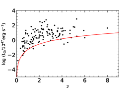
(a)

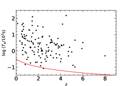
(b)

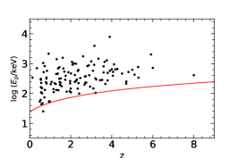
(c)

Figure 12: The distribution of the 121 GRBs on the $L_{X}-z$ plane (left panel), the $T_{a}-z$ plane (middle panel), and the $E_{\rm{p}}-z$ plane (right panel). The solid curves correspond to $F_{X,\rm{lim}}=1.0\times 10^{-12}$ erg cm², $T_{a,\rm{lim}}=309/(1+z)$ s and $E_{\rm{p,lim}}=1.39\times(1+z)$ keV, respectively.

Then, for the $i$th data $(L_{X,i},z_{i})$ in the GRB sample, we can define its associated set as

$$J_{i}=\{j|L_{X,j}>L_{i},\;\rm{and}\;z_{j}<z_{i,\rm{lim}}\},$$ (A1)

where $z_{i,\rm{lim}}$ is the redshift corresponding to the flux threshold for a GRB of $(L_{X,i},z_{i})$. For each data point in the sample, we can define its associated set $J_{i}$, and the number of GRBs in the set is counted as $N_{i}$. Also, we can get its rank $R_{i}$ in its associated set $J_{i}$ as,

$$R_{i}=\rm{number}\{j\in J_{i}|z_{j}\geq z_{i}\}.$$ (A2)

The key point of this method is to determine the rank $R_{i}$ for each data point in its associated set. If $L_{X}$ and $z$ are independent, $R_{i}$ should be uniformly distributed between 1 and $N_{i}$ (Efron & Petrosian, 1992). The test statistic $\tau$ is

$$\tau=\frac{\sum_{i}(R_{i}-E_{i})}{\sqrt{\sum_{i}V_{i}}},$$ (A3)

where $E_{i}=(N_{i}+1)/2$ and $V_{i}=(N_{i}^{2}-1)/12$ are the expected mean and the variance of $R_{i}$ respectively. If $R_{i}$ is uniformly distributed between 1 and $N_{i}$, then the value of $\tau$ should equal to zero. In other words, we need to find the value of $k_{L_{X}}$ for which $\tau_{L_{X}}=0$, where $\tau_{L_{X}}$ is calculated by using the $(L^{\prime}_{X},z)$ data set.

The best $k_{L_{X}}$ we derived is $k_{L_{X}}=3.38\pm 0.62$. Using the same method, we get $k_{T_{a}}=-1.54\pm 0.30$ and $k_{E_{\rm{p}}}=0.75\pm 0.25$. The $1\sigma$ range of uncertainty is derived from $|\tau_{x}|\leq 1$ ($x=L_{X},T_{a},E_{\rm{p}}$). These $k$ values represent the evolution indices for $L_{X}$, $T_{a}$, and $E_{\rm{p}}$, respectively. In Figure 13 below, for clarity, we have plotted $\tau$ versus $k$ for the three parameters.

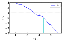
(a)

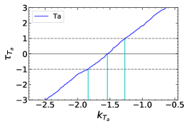
(b)

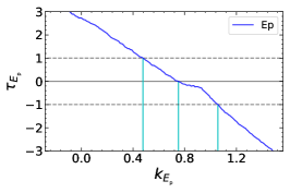
(c)

Figure 13: The relation between $\tau_{L_{X}}-k_{L_{X}}$ (left panel), $\tau_{T_{a}}-k_{T_{a}}$ (middle panel), and $\tau_{E_{\rm{p}}}-k_{E_{\rm{p}}}$ (right panel). The best $k$ value is determined by $\tau=0$, and the $1\sigma$ range of uncertainty is derived from $|\tau|\leq 1$.

References

- Abbott et al. (2019) Abbott, T. M. C., Allam, S., Andersen, P., et al. 2019, ApJ, 872, L30, doi: 10.3847/2041-8213/ab04fa
- Alam et al. (2017) Alam, S., Ata, M., Bailey, S., et al. 2017, MNRAS, 470, 2617, doi: 10.1093/mnras/stx721
- Amati et al. (2019) Amati, L., D’Agostino, R., Luongo, O., Muccino, M., & Tantalo, M. 2019, MNRAS, 486, L46, doi: 10.1093/mnrasl/slz056
- Amati et al. (2008) Amati, L., Guidorzi, C., Frontera, F., et al. 2008, MNRAS, 391, 577, doi: 10.1111/j.1365-2966.2008.13943.x
- Amati et al. (2002) Amati, L., Frontera, F., Tavani, M., et al. 2002, A&A, 390, 81, doi: 10.1051/0004-6361:20020722
- Bernardini et al. (2012) Bernardini, M. G., Margutti, R., Zaninoni, E., & Chincarini, G. 2012, MNRAS, 425, 1199, doi: 10.1111/j.1365-2966.2012.21487.x
- Betoule et al. (2014) Betoule, M., Kessler, R., Guy, J., et al. 2014, A&A, 568, A22, doi: 10.1051/0004-6361/201423413
- Cardone et al. (2009) Cardone, V. F., Capozziello, S., & Dainotti, M. G. 2009, MNRAS, 400, 775, doi: 10.1111/j.1365-2966.2009.15456.x
- Cardone et al. (2010) Cardone, V. F., Dainotti, M. G., Capozziello, S., & Willingale, R. 2010, MNRAS, 408, 1181, doi: 10.1111/j.1365-2966.2010.17197.x
- Cucchiara et al. (2011) Cucchiara, A., Levan, A. J., Fox, D. B., et al. 2011, ApJ, 736, 7, doi: 10.1088/0004-637X/736/1/7
- D’Agostini (2005) D’Agostini, G. 2005, arXiv e-prints, physics/0511182. https://arxiv.org/abs/physics/0511182
- Dai et al. (2004) Dai, Z. G., Liang, E. W., & Xu, D. 2004, ApJ, 612, L101, doi: 10.1086/424694
- Dainotti (2019) Dainotti, M. 2019, Gamma-ray Burst Correlations, 2053-2563 (IOP Publishing), doi: 10.1088/2053-2563/aae15c
- Dainotti et al. (2015) Dainotti, M., Petrosian, V., Willingale, R., et al. 2015, MNRAS, 451, 3898, doi: 10.1093/mnras/stv1229
- Dainotti & Amati (2018) Dainotti, M. G., & Amati, L. 2018, PASP, 130, 051001, doi: 10.1088/1538-3873/aaa8d7
- Dainotti et al. (2008) Dainotti, M. G., Cardone, V. F., & Capozziello, S. 2008, MNRAS, 391, L79, doi: 10.1111/j.1745-3933.2008.00560.x
- Dainotti et al. (2013a) Dainotti, M. G., Cardone, V. F., Piedipalumbo, E., & Capozziello, S. 2013a, MNRAS, 436, 82, doi: 10.1093/mnras/stt1516
- Dainotti & Del Vecchio (2017) Dainotti, M. G., & Del Vecchio, R. 2017, New A Rev., 77, 23, doi: 10.1016/j.newar.2017.04.001
- Dainotti et al. (2018) Dainotti, M. G., Del Vecchio, R., & Tarnopolski, M. 2018, Advances in Astronomy, 2018, 4969503, doi: 10.1155/2018/4969503
- Dainotti et al. (2011) Dainotti, M. G., Fabrizio Cardone, V., Capozziello, S., Ostrowski, M., & Willingale, R. 2011, ApJ, 730, 135, doi: 10.1088/0004-637X/730/2/135
- Dainotti et al. (2017a) Dainotti, M. G., Hernandez, X., Postnikov, S., et al. 2017a, ApJ, 848, 88, doi: 10.3847/1538-4357/aa8a6b
- Dainotti et al. (2020) Dainotti, M. G., Lenart, A. Ł., Sarracino, G., et al. 2020, ApJ, 904, 97, doi: 10.3847/1538-4357/abbe8a
- Dainotti et al. (2017b) Dainotti, M. G., Nagataki, S., Maeda, K., Postnikov, S., & Pian, E. 2017b, A&A, 600, A98, doi: 10.1051/0004-6361/201628384
- Dainotti et al. (2013b) Dainotti, M. G., Petrosian, V., Singal, J., & Ostrowski, M. 2013b, ApJ, 774, 157, doi: 10.1088/0004-637X/774/2/157
- Dainotti et al. (2016) Dainotti, M. G., Postnikov, S., Hernandez, X., & Ostrowski, M. 2016, ApJ, 825, L20, doi: 10.3847/2041-8205/825/2/L20
- Dainotti et al. (2010) Dainotti, M. G., Willingale, R., Capozziello, S., Fabrizio Cardone, V., & Ostrowski, M. 2010, ApJ, 722, L215, doi: 10.1088/2041-8205/722/2/L215
- Dall’Osso et al. (2011) Dall’Osso, S., Stratta, G., Guetta, D., et al. 2011, A&A, 526, A121, doi: 10.1051/0004-6361/201014168
- Del Vecchio et al. (2016) Del Vecchio, R., Dainotti, M. G., & Ostrowski, M. 2016, ApJ, 828, 36, doi: 10.3847/0004-637X/828/1/36
- Demianski et al. (2017) Demianski, M., Piedipalumbo, E., Sawant, D., & Amati, L. 2017, A&A, 598, A112, doi: 10.1051/0004-6361/201628909
- Demianski et al. (2019) —. 2019, arXiv e-prints, arXiv:1911.08228. https://arxiv.org/abs/1911.08228
- Deng et al. (2016) Deng, C.-M., Wang, X.-G., Guo, B.-B., et al. 2016, ApJ, 820, 66, doi: 10.3847/0004-637X/820/1/66
- Efron & Petrosian (1992) Efron, B., & Petrosian, V. 1992, ApJ, 399, 345, doi: 10.1086/171931
- Eisenstein et al. (2005) Eisenstein, D. J., Zehavi, I., Hogg, D. W., et al. 2005, ApJ, 633, 560, doi: 10.1086/466512
- Evans et al. (2009) Evans, P. A., Beardmore, A. P., Page, K. L., et al. 2009, MNRAS, 397, 1177, doi: 10.1111/j.1365-2966.2009.14913.x
- Fenimore & Ramirez-Ruiz (2000) Fenimore, E. E., & Ramirez-Ruiz, E. 2000, arXiv e-prints, astro. https://arxiv.org/abs/astro-ph/0004176
- Firmani et al. (2006) Firmani, C., Ghisellini, G., Avila-Reese, V., & Ghirland a, G. 2006, MNRAS, 370, 185, doi: 10.1111/j.1365-2966.2006.10445.x
- Ghirlanda et al. (2006) Ghirlanda, G., Ghisellini, G., & Firmani, C. 2006, New Journal of Physics, 8, 123, doi: 10.1088/1367-2630/8/7/123
- Ghirlanda et al. (2004) Ghirlanda, G., Ghisellini, G., & Lazzati, D. 2004, ApJ, 616, 331, doi: 10.1086/424913
- Gruber et al. (2014) Gruber, D., Goldstein, A., Weller von Ahlefeld, V., et al. 2014, ApJS, 211, 12, doi: 10.1088/0067-0049/211/1/12
- Izzo et al. (2015) Izzo, L., Muccino, M., Zaninoni, E., Amati, L., & Della Valle, M. 2015, A&A, 582, A115, doi: 10.1051/0004-6361/201526461
- Li et al. (2018) Li, L., Wu, X.-F., Lei, W.-H., et al. 2018, ApJS, 236, 26, doi: 10.3847/1538-4365/aabaf3
- Li et al. (2012) Li, L., Liang, E.-W., Tang, Q.-W., et al. 2012, ApJ, 758, 27, doi: 10.1088/0004-637X/758/1/27
- Liang & Zhang (2005) Liang, E., & Zhang, B. 2005, ApJ, 633, 611, doi: 10.1086/491594
- Liang et al. (2008) Liang, N., Xiao, W. K., Liu, Y., & Zhang, S. N. 2008, ApJ, 685, 354, doi: 10.1086/590903
- Lien et al. (2016) Lien, A., Sakamoto, T., Barthelmy, S. D., et al. 2016, ApJ, 829, 7, doi: 10.3847/0004-637X/829/1/7
- Lin et al. (2016) Lin, H.-N., Li, X., & Chang, Z. 2016, MNRAS, 455, 2131, doi: 10.1093/mnras/stv2471
- Luongo & Muccino (2020a) Luongo, O., & Muccino, M. 2020a, A&A, 641, A174, doi: 10.1051/0004-6361/202038264
- Luongo & Muccino (2020b) —. 2020b, arXiv e-prints, arXiv:2011.13590. https://arxiv.org/abs/2011.13590
- Lusso et al. (2019) Lusso, E., Piedipalumbo, E., Risaliti, G., et al. 2019, A&A, 628, L4, doi: 10.1051/0004-6361/201936223
- Minaev & Pozanenko (2020) Minaev, P. Y., & Pozanenko, A. S. 2020, MNRAS, 492, 1919, doi: 10.1093/mnras/stz3611
- Muccino et al. (2021) Muccino, M., Izzo, L., Luongo, O., et al. 2021, ApJ, 908, 181, doi: 10.3847/1538-4357/abd254
- Narayana Bhat et al. (2016) Narayana Bhat, P., Meegan, C. A., von Kienlin, A., et al. 2016, ApJS, 223, 28, doi: 10.3847/0067-0049/223/2/28
- Norris et al. (2000) Norris, J. P., Marani, G. F., & Bonnell, J. T. 2000, ApJ, 534, 248, doi: 10.1086/308725
- Perlmutter et al. (1999) Perlmutter, S., Aldering, G., Goldhaber, G., et al. 1999, ApJ, 517, 565, doi: 10.1086/307221
- Petrosian et al. (2015) Petrosian, V., Kitanidis, E., & Kocevski, D. 2015, ApJ, 806, 44, doi: 10.1088/0004-637X/806/1/44
- Phillips (1993) Phillips, M. M. 1993, ApJ, 413, L105, doi: 10.1086/186970
- Planck Collaboration et al. (2014) Planck Collaboration, Ade, P. A. R., Aghanim, N., et al. 2014, A&A, 571, A16, doi: 10.1051/0004-6361/201321591
- Planck Collaboration et al. (2016) —. 2016, A&A, 594, A13, doi: 10.1051/0004-6361/201525830
- Planck Collaboration et al. (2020) Planck Collaboration, Aghanim, N., Akrami, Y., et al. 2020, A&A, 641, A6, doi: 10.1051/0004-6361/201833910
- Postnikov et al. (2014) Postnikov, S., Dainotti, M. G., Hernandez, X., & Capozziello, S. 2014, ApJ, 783, 126, doi: 10.1088/0004-637X/783/2/126
- Rea et al. (2015) Rea, N., Gullón, M., Pons, J. A., et al. 2015, ApJ, 813, 92, doi: 10.1088/0004-637X/813/2/92
- Reichart (2001) Reichart, D. E. 2001, ApJ, 553, 235, doi: 10.1086/320630
- Riess et al. (2019) Riess, A. G., Casertano, S., Yuan, W., Macri, L. M., & Scolnic, D. 2019, ApJ, 876, 85, doi: 10.3847/1538-4357/ab1422
- Riess et al. (1998) Riess, A. G., Filippenko, A. V., Challis, P., et al. 1998, AJ, 116, 1009, doi: 10.1086/300499
- Risaliti & Lusso (2019) Risaliti, G., & Lusso, E. 2019, Nature Astronomy, 3, 272, doi: 10.1038/s41550-018-0657-z
- Rowlinson et al. (2014) Rowlinson, A., Gompertz, B. P., Dainotti, M., et al. 2014, MNRAS, 443, 1779, doi: 10.1093/mnras/stu1277
- Ruffini et al. (2014) Ruffini, R., Muccino, M., Bianco, C. L., et al. 2014, A&A, 565, L10, doi: 10.1051/0004-6361/201423812
- Sánchez et al. (2017) Sánchez, A. G., Grieb, J. N., Salazar-Albornoz, S., et al. 2017, MNRAS, 464, 1493, doi: 10.1093/mnras/stw2495
- Schaefer (2007) Schaefer, B. E. 2007, ApJ, 660, 16, doi: 10.1086/511742
- Scolnic et al. (2018) Scolnic, D. M., Jones, D. O., Rest, A., et al. 2018, ApJ, 859, 101, doi: 10.3847/1538-4357/aab9bb
- Singal et al. (2011) Singal, J., Petrosian, V., Lawrence, A., & Stawarz, Ł. 2011, ApJ, 743, 104, doi: 10.1088/0004-637X/743/2/104
- Spergel et al. (2003) Spergel, D. N., Verde, L., Peiris, H. V., et al. 2003, ApJS, 148, 175, doi: 10.1086/377226
- Stratta et al. (2018) Stratta, G., Dainotti, M. G., Dall’Osso, S., Hernandez, X., & De Cesare, G. 2018, ApJ, 869, 155, doi: 10.3847/1538-4357/aadd8f
- Tang et al. (2019) Tang, C.-H., Huang, Y.-F., Geng, J.-J., & Zhang, Z.-B. 2019, ApJS, 245, 1, doi: 10.3847/1538-4365/ab4711
- Tu et al. (2019) Tu, Z. L., Hu, J., & Wang, F. Y. 2019, MNRAS, 484, 4337, doi: 10.1093/mnras/stz286
- von Kienlin et al. (2014) von Kienlin, A., Meegan, C. A., Paciesas, W. S., et al. 2014, ApJS, 211, 13, doi: 10.1088/0067-0049/211/1/13
- von Kienlin et al. (2020) —. 2020, ApJ, 893, 46, doi: 10.3847/1538-4357/ab7a18
- Wang et al. (2020) Wang, F., Zou, Y.-C., Liu, F., et al. 2020, ApJ, 893, 77, doi: 10.3847/1538-4357/ab0a86
- Wang et al. (2015) Wang, F. Y., Dai, Z. G., & Liang, E. W. 2015, New A Rev., 67, 1, doi: 10.1016/j.newar.2015.03.001
- Wang et al. (2017) Wang, G.-J., Yu, H., Li, Z.-X., Xia, J.-Q., & Zhu, Z.-H. 2017, ApJ, 836, 103, doi: 10.3847/1538-4357/aa5b9b
- Wang et al. (2016) Wang, J. S., Wang, F. Y., Cheng, K. S., & Dai, Z. G. 2016, A&A, 585, A68, doi: 10.1051/0004-6361/201526485
- Wang & Dai (2016) Wang, Y., & Dai, M. 2016, Phys. Rev. D, 94, 083521, doi: 10.1103/PhysRevD.94.083521
- Wang & Mukherjee (2006) Wang, Y., & Mukherjee, P. 2006, ApJ, 650, 1, doi: 10.1086/507091
- Wang & Wang (2019) Wang, Y. Y., & Wang, F. Y. 2019, ApJ, 873, 39, doi: 10.3847/1538-4357/ab037b
- Xu & Huang (2012) Xu, M., & Huang, Y. F. 2012, A&A, 538, A134, doi: 10.1051/0004-6361/201117754
- Yi et al. (2016) Yi, S.-X., Xi, S.-Q., Yu, H., et al. 2016, ApJS, 224, 20, doi: 10.3847/0067-0049/224/2/20
- Yonetoku et al. (2004) Yonetoku, D., Murakami, T., Nakamura, T., et al. 2004, ApJ, 609, 935, doi: 10.1086/421285
- Yu et al. (2015) Yu, H., Wang, F. Y., Dai, Z. G., & Cheng, K. S. 2015, ApJS, 218, 13, doi: 10.1088/0067-0049/218/1/13
- Zhang (2011) Zhang, B. 2011, Comptes Rendus Physique, 12, 206, doi: 10.1016/j.crhy.2011.03.004
- Zhao et al. (2019) Zhao, L., Zhang, B., Gao, H., et al. 2019, ApJ, 883, 97, doi: 10.3847/1538-4357/ab38c4