Fluctuation profiles in inhomogeneous fluids

Abstract

Three one-body profiles that correspond to local fluctuations in energy, in entropy, and in particle number are used to describe the equilibrium properties of inhomogeneous classical many-body systems. Local fluctuations are obtained from thermodynamic differentiation of the density profile or equivalently from average microscopic covariances. The fluctuation profiles follow from functional generators and they satisfy Ornstein-Zernike relations. Computer simulations reveal markedly different fluctuations in confined fluids with Lennard-Jones, hard sphere, and Gaussian core interactions.

Inhomogeneous fluids comprise a large class of relevant and fundamental physical systems, in which a broad range of phenomena and underlying mechanisms occur hansen2013 ; evans1979 ; evans2016specialIssue . Examples include the behaviour of fluids in narrow confinement nygard2016prx , electrolytes near surfaces martinjimenez2017natCom , dense fluid structuring as revealed in atomic force microscopy hernandez-munoz2019 , thermal resistance of liquid-vapor interfaces muscatello2017 , nonequilibrium steady states in active paliwal2018 ; rodenburg2018 , sheared brader2011shear and driven scacchi2018 fluids, as well as the orientation-resolved ordering of water around complex solutes jeanmairet2013jcp ; jeanmairet2013jpcl ; levesque2012jcp ; sergiievskyi2014 ; jeanmairet2019capacitor . The average one-body density distribution, or short the density profile, is used as the standard tool for analyzing such inhomogeneous systems.

In particular the occurrence of hydrophobicity levesque2012jcp ; jeanmairet2013jcp ; stewart2012pre ; stewart2014jcp ; evans2015jpcm ; evans2015prl ; chacko2017 ; evans2017 ; evans2019pnas ; rensing2019pnas ; evans2016prl ; giacomello2016 ; giacomello2019 , and its important consequences in biological systems, have been at the center of much current scientific attention and debate. At hydrophobic substrates or around hydrophobic solutes, water avoids contact of its liquid phase. In the more general framework of solvophobicity (where the liquid is not necessarily water), Evans and coworkers argue stewart2012pre ; stewart2014jcp ; evans2015jpcm ; evans2015prl ; chacko2017 ; evans2017 ; evans2019pnas ; rensing2019pnas ; evans2016prl that the local compressibility is a more suitable indicator of the occurrence of drying than is the bare density profile. These authors obtain (and define) the local compressibility $\chi_{\mu}({\bf r})$ by differentiating the density profile, $\rho({\bf r})$, with respect to the chemical potential, $\mu$, in straightforward generalization of the definition of the bulk compressibility; they also use correlators and reweighting to obtain $\chi_{\mu}({\bf r})$. At a planar substrate $\chi_{\mu}({\bf r})$ measures in-plane density fluctuations and the results show a very pronounced signal when a drying film develops near the substrate. The findings of Refs. stewart2012pre ; stewart2014jcp ; evans2015jpcm ; evans2015prl ; chacko2017 ; evans2017 ; evans2019pnas ; rensing2019pnas ; evans2016prl , obtained over a range of microscopic models (differently truncated Lennard-Jones particles, as well as classical models for water) convincingly demonstrate the superiority of $\chi_{\mu}({\bf r})$ over $\rho({\bf r})$ as an indicator function for the occurring physics.

From a fundamental point of view, and in particular that of classical density functional theory evans1979 ; hansen2013 ; evans2016specialIssue (DFT) where $\rho({\bf r})$ is the central (variational) variable, the above situation is perplexing, and it is unclear whether the observation is merely relevant for the particular situations they consider or whether it is indicative of a more general underlying theoretical structure.

Here we show that the latter is the case, when the local compressibility $\chi_{\mu}({\bf r})$ is complemented by two further local measures of fluctuations. One of these additional fields is the local thermal susceptibility $\chi_{T}({\bf r})$, which constitutes the partial derivative with respect to temperature $T$ of the density profile. As we demonstrate below, $\chi_{T}({\bf r})$ is indicative of entropic correlation effects. It is then natural to also consider a reduced density profile $\chi_{\star}({\bf r})$, where the thermal and chemical fluctuations have been subtracted. Hence

$$\chi_{\mu}({\bf r}) =\frac{\partial\rho({\bf r})}{\partial\mu}\Big{|}_{T},$$ (1)

$$\chi_{T}({\bf r}) =\frac{\partial\rho({\bf r})}{\partial T}\Big{|}_{\mu},$$ (2)

$$\chi_{\star}({\bf r}) =\rho({\bf r})-\mu\frac{\partial\rho({\bf r})}{\partial\mu}\Big{|}_{T}-T\frac{\partial\rho({\bf r})}{\partial T}\Big{|}_{\mu}$$ (3)

$$\equiv\rho({\bf r})-\mu\chi_{\mu}({\bf r})-T\chi_{T}({\bf r}),$$ (4)

where the external potential $V_{\rm ext}({\bf r})$ is kept constant under the partial thermodynamic derivatives. Equation (3) is akin to a Legendre transform of the density profile with respect to the thermodynamic variables $T$ and $\mu$, and (4) is obtained from (3) by using (1) and (2).

Given the relationships of the three fluctuation profiles $\chi_{a}({\bf r})$, $a=\mu,T,\star$ to the density profile (1)–(3), we demonstrate three further fundamental properties: i) Representation as explicit correlation functions, given as ensemble averages, which makes all three correlators directly accessible in particle-based simulations via averaging. ii) All three fluctuation profiles can be generated as response functions to changes in the external potential $V_{\rm ext}({\bf r})$. iii) The fluctuation profiles satisfy Ornstein-Zernike (OZ) relations, which remarkably have simpler structure than the standard (inhomogeneous) OZ relation evans1979 ; hansen2013 ; ornstein1914 . We demonstrate, based on computer simulation data, that the fluctuation profiles are highly sensitive to the type of interparticle interactions, and that they display markedly different behaviour for different model fluids.

Recall that the density profile $\rho({\bf r})$ measures the microscopically resolved mean number of particles at position ${\bf r}$. Its integral over the system volume $V$ yields the average total number of particles, $\bar{N}=\int_{V}d{\bf r}\rho({\bf r})$, and for bulk fluids $\rho({\bf r})=\rho_{b}=\rm const$, where $\rho_{b}=\bar{N}/V$ is the bulk fluid (number) density. In the grand ensemble, when the system is coupled to a heat bath at temperature $T$ and to a particle bath at chemical potential $\mu$, then $\rho_{b}(T,\mu)$ represents a fundamental equation of state of the bulk liquid, from which all further thermodynamic quantities can be obtained. Differentiation of $\rho_{b}$ with respect to the thermodynamic variables yields the bulk thermal susceptibility when changing temperature, $\chi_{T}^{b}=\partial\rho_{b}/\partial T|_{\mu}$, and the isothermal compressibility when changing the chemical potential, $\chi_{\mu}^{b}=\partial\rho_{b}/\partial\mu|_{T}$. Hence $\chi_{\mu}^{b}$ has the status of a chemical susceptibility. The respective right hand sides imply that $\chi_{T}^{b}$ and $\chi_{\mu}^{b}$ are global response functions that characterize the ease (or lack thereof) to influence the bulk density upon changing the control parameter of either bath.

To be specific, we consider Hamiltonians of the form $\hat{H}=\hat{K}+u({\bf r}^{N})+\sum_{i}V_{\rm ext}({\bf r}_{i})$, where $\hat{K}$ indicates kinetic energy and $u({\bf r}^{N})$ denotes the interparticle interaction potential that depends on all $N$ particle positions ${\bf r}^{N}\equiv{\bf r}_{1}\ldots{\bf r}_{N}$, where ${\bf r}_{i}$ is the position of particle $i=1\ldots N$ in $D$ spatial dimensions. In order to resolve the density locally it is common to introduce the density operator $\hat{\rho}({\bf r})=\sum_{i}\delta({\bf r}-{\bf r}_{i})$. The density profile is then obtained as the average $\rho({\bf r})=\langle\hat{\rho}({\bf r})\rangle$, where the angular brackets denote an average over microstates that are distributed according to the (grand canonical) equilibrium distribution function $\Psi=\exp(-\beta(\hat{H}-\mu N))/\Xi$, where $\beta=1/(k_{B}T)$, with $k_{B}$ indicating the Boltzmann constant and $\Xi$ the grand canonical partition sum.

We start by considering correlators, i.e. ensemble averages over suitable many-body (phase space) functions. Differentiating the density profile in the form $\rho({\bf r})=\langle\hat{\rho}({\bf r})\rangle$ with respect to the thermodynamic parameters according to (1) and (2) naturally leads to results that are of covariance form. We indicate the covariance of two operators (phase space functions) $\hat{A}$ and $\hat{B}$ as ${\,\rm cov}(\hat{A},\hat{B})=\langle\hat{A}\hat{B}\rangle-\langle\hat{A}\rangle\langle\hat{B}\rangle$. We obtain

$$\chi_{\mu}({\bf r}) =\beta{\,\rm cov}(N,\hat{\rho}),$$ (5)

$$\chi_{T}({\bf r}) =\beta{\,\rm cov}(\hat{S},\hat{\rho})$$ (6)

$$\equiv\beta{\,\rm cov}(\hat{H}-\mu N,\hat{\rho})/T,$$ (7)

$$\chi_{\star}({\bf r}) =\rho({\bf r})-\beta{\,\rm cov}(\hat{H},\hat{\rho}),$$ (8)

where $\hat{S}=-k_{B}\ln\Psi$ is the entropy operator, such that $S=\langle\hat{S}\rangle$ is the total entropy. The form (5) has been given before in Refs. evans2015prl ; evans2017 , while (7) is obtained by inserting the explicit Boltzmann form of $\Psi$ into (6). Crucially (7) can be carried out via importance sampling in particle-based simulations (which is hampered in (6) due to the poor direct accessibility of $\ln\Psi$). Note that (6) is different from the entropy density $\langle\hat{\rho}\hat{S}/N\rangle$ of Ref. schmidt2011pre . It becomes apparent that (3) leads to (8), which constitutes a reduced density distribution, where the energy-density covariance is subtracted from the full density profile.

Figure 1: Normalized fluctuation profiles $\chi_{a}(x)/\chi_{a}^{b}$, where $a=\mu,T,\star$, for the LJ liquid (a,b), the HS fluid (c), and the GCM (d). Results are for fluids confined between a planar 3-9 LJ wall (left) and a planar hard wall (right) (a,c,d) and for the LJ free gas-liquid interface (b). Shown are results for $\chi_{T}$ (orange solid line), $\chi_{\mu}$ (blue dashed line) and $\chi_{\star}$ (purple dotted line) as a function of distance $x/\sigma$ across the slit and normalized by the respective bulk value. The insets in (a,c,d) show the corresponding density profile $\rho(x)\sigma^{3}$ (solid green line) and replot the (non-normalized) reduced density profiles $\chi_{\star}(x)\sigma^{3}$ using either convention for $\Lambda$ in (a) (as indicated); the results in (b,c,d) are for $\Lambda=\sigma$; The bulk values are $\chi_{T}^{b}\epsilon\sigma^{3}/k_{B}=-0.640$ (a), $-0.217$ (c), 0.082 (d); $\chi_{\mu}^{b}\epsilon\sigma^{3}=0.092$ (a), 0.065 (c), 0.063 (d), and $\chi_{\star}^{b}\sigma^{3}=1.553$ (a), 0.515 (c), 0.051 (d) for $\Lambda=\sigma$; for $\Lambda(T)$ in (a): $\chi_{T}^{b}\epsilon\sigma^{3}/k_{B}=0.432$ and $\chi_{\star}^{b}\sigma^{3}=1.435$.

For the ideal gas ($u\equiv 0$) one can show $\chi_{\mu}^{\rm id}({\bf r})=\beta\rho({\bf r})$ and also obtain closed forms for $\chi_{T}({\bf r})$ and $\chi_{\star}({\bf r})$ SMchilocal . Turning to interacting systems, we first consider the Lennard-Jones (LJ) liquid confined in an asymmetric planar slit pore, which consists of two opposing walls, inspired by Ref. evans2015jpcm . We use grand canonical Monte Carlo simulations in $D=3$ dimensions, with simulation box dimensions $L_{x}=15\sigma$ and $L_{y}=L_{z}=6\sigma$ and periodic boundaries in the $y$- and $z$-directions. Here $\sigma$ is the LJ length scale. We equilibrate for $\geq 10^{7}$ grandcanonical MC moves before sampling data $10^{8}-10^{9}$ times, with $100-300$ trial moves between consecutive samples. We consider a 3-9 LJ wall at $x=0$, described by an external potential $V_{\rm ext}^{\rm LJ}(x)=(\epsilon_{w}/2)[(\zeta/x)^{9}-3(\zeta/x)^{3}]$, where the range $\zeta$ is set to $\zeta=0.95\sigma$ evans2015jpcm . The strength is chosen as $\epsilon_{w}=0.49\epsilon$, where $\epsilon$ is the LJ energy scale. This value of $\epsilon_{w}$ corresponds to a weakly attractive wall; it is intermediate between the solvophobic and neutral cases of Ref. evans2015jpcm . Both $V_{\rm ext}^{\rm LJ}(x)$ and the LJ pair potential are cut and shifted hansen2013 at a cutoff distance $2.5\sigma$. The second wall is hard and located at $x=L_{x}$, such that no particle center can go beyond that distance. We choose a statepoint on the liquid side of the gas-liquid binodal: $k_{B}T=0.85\epsilon$ and $\tilde{\mu}=-2.90\epsilon$; here we use a reduced chemical potential with the kinetic contribution subtracted, $\tilde{\mu}\equiv\mu-k_{B}TD\ln(\Lambda/\sigma)$, where $\Lambda$ indicates the thermal de Broglie wavelength.

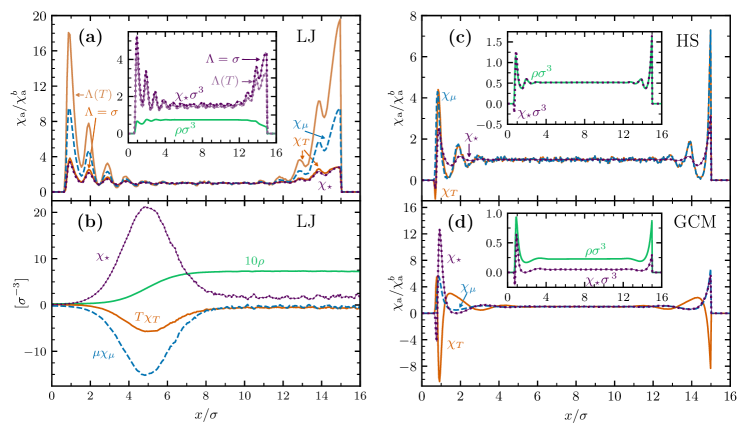
Fig. 1(a) illustrates the resulting behaviour of the three fluctuation profiles $\chi_{\mu}(x)$, $\chi_{T}(x)$, and $\chi_{\star}(x)$. The density profile $\rho(x)$ of the LJ liquid near each wall displays depletion (negative adsorption) characteristic of solvophobic substrates stewart2012pre ; stewart2014jcp ; evans2015jpcm ; evans2015prl ; chacko2017 ; evans2017 ; evans2019pnas ; rensing2019pnas ; evans2016prl , cf. the inset in Fig. 1(a). As reported by Evans and coworkers, $\chi_{\mu}(x)$ is indeed a better indicator for the emergence of drying than $\rho(x)$ is. To see this, consider that the amplitude of the signal, i.e. the enhancement of local fluctuations over the bulk that is apparent in $\chi_{\mu}$, but also in $\chi_{T}$ and in $\chi_{\star}$ (main plot of Fig. 1(a)) is quantitatively much stronger than the small depletion effect that occurs in the local density near the wall (inset in Fig. 1(a)). This sensitivity is intimately linked to the thermodynamic derivative structure (1)–(3), which, in a Taylor series sense, probes the local environment around statepoint $T,\mu$. Clearly, this provides a mechanism to sense the proximity of a phase transition. We have checked that both routes to the fluctuation profiles, via thermodynamic differentiation according to (1) and (2), as well as covariance sampling according to (5) and (7) give identical results within numerical accuracy. In Fig. 1, each fluctuation profile $\chi_{a}(x)$ is normalized by its respective bulk value, $\chi_{a}^{b}$, which we obtain consistently from either an independent bulk simulation run (without external potential and with periodic boundaries in all three spatial directions) or from the plateau value at the center of the slit.

Remarkably, $\chi_{T}(x)$ also displays a very strong response near each wall; recall that this quantity is indicative of entropic correlation effects, cf. (6). Notably, the entropic fluctuations are much increased when the full temperature dependence is taken into account, cf. the stronger signal of $\chi_{T}(x)$ when using $\Lambda(T)$ SMchilocal (light orange line), as compared to $\Lambda=\sigma$ (dark orange line). The reduced density $\chi_{\star}(x)$ acquires much oscillatory behaviour (see inset in Fig. 1(a)) and it possesses a form that is markedly different from the density profile $\rho(x)$, in the present case of the LJ system. Note that either convention for $\Lambda$ carries the full information. Upon changing the convention for $\Lambda$ from $\sigma\to\Lambda(T)$, the fluctuation profiles acquire kinetic terms according to $\chi_{T}({\bf r})\to\chi_{T}({\bf r})+k_{B}D\chi_{\mu}({\bf r})/2$ and $\chi_{\star}({\bf r})\to\chi_{\star}({\bf r})-k_{B}TD\chi_{\mu}({\bf r})/2$, with $\rho({\bf r})$ and $\chi_{\mu}({\bf r})$ remaining unchanged. We adhere to $\Lambda=\sigma$ in the following (which implies considering only configurational contributions in (6)–(8)).

The fluctuation profiles at a (quasi-)free gas-liquid interface in the LJ system are shown in Fig. 1(b). In order to stabilize gas-liquid coexistence in our grand canonical simulation setup, we use a weak and slowly oscillating external potential, $V_{\rm ext}(x)=0.2\epsilon\cos\left(2\pi x/L_{x}\right)$, such that the local chemical potential $\tilde{\mu}-V_{\mathrm{ext}}(x)$ crosses over from the gas to the liquid side of the gas-liquid binodal. We use a periodic simulation box that is extendend in the $x$-direction to $L_{x}=25\sigma$ and choose $\tilde{\mu}=-3.2\epsilon$ and $k_{B}T=0.85\epsilon$. All three $\chi_{a}(x)$ display a marked signal at the interface.

Returning to the asymmetric slit pore, we next consider a confined fluid of hard spheres (HS) of diameter $\sigma$. Results for the statepoint $k_{B}T=1\epsilon$ and $\tilde{\mu}=3.36\epsilon$ are shown in Fig. 1(c). At the planar hard wall davidchack2016 ; roth2010review at $x=15\sigma$, and more generally when all interactions are of hard core type, the fluctuation profiles simplify, as both interparticle and external potential energy vanish for all allowed microstates. Comparing the resulting form of the thermal susceptibility (7) with the definition of the chemical susceptibility (local compressibility) (5) yields the (hard core) identity $T\chi_{T}({\bf r})=\mu\chi_{\mu}({\bf r})$. Furthermore, if all (internal and external) interactions are hard core, the reduced density (8) remarkably simplifies to $\chi_{\star}({\bf r})=\rho({\bf r})$. (Kinetic terms can be regained by transforming to $\Lambda(T)$ as described above.) The results shown in Fig. 1(c) confirm these properties and illustrate the spatial variation of the fluctuation fields both at the hard wall and the soft LJ wall. For hard spheres and soft external potentials, it is straightforward to show from (8) that $\chi_{\star}({\bf r})=\rho({\bf r})-\beta\int d{\bf r}^{\prime}V_{\rm ext}({\bf r}^{\prime}){\,\rm cov}(\hat{\rho}({\bf r}),\hat{\rho}({\bf r}^{\prime}))$. Note that the covariance is a fundamental correlator of density fluctuations hansen2013 ; evans1979 .

To further assess how specific the fluctuation profiles are to the particular type of model fluid, we consider the Gaussian core model (GCM) stillinger1976 ; archer2001 ; archer2002 , where particles are allowed to penetrate each other at a finite energy cost. The interparticle interaction potential has a Gaussian form, $\phi_{\mathrm{GCM}}(r)=\epsilon{\rm e}^{-r^{2}/(2\sigma^{2})}$; we cut off and shift at a distance of $3\sigma$. Results for the fluctuation profiles of the GCM are shown in Fig. 1(d), for $\tilde{\mu}=2.16\epsilon$ and $k_{B}T=0.5\epsilon$. The profiles differ very markedly from those of both the LJ and HS cases. Note in particular the sign change of $\chi_{T}(x)$ as compared to the HS case shown in Fig. 1(c). In summary, on the basis of the simulation data, we conclude that all three fluctuation profiles are highly useful quantitative indicators of molecular structuring phenomena over and beyond the density profile. Of course, Fig. 1(a) and (b) are most revealing since the density profile is fairly smooth whereas the other profiles show considerable structure.

We next turn to addressing the fundamental status of the fluctuation profiles in more depth. In order to do so, we resort to classical DFT as the primary modern framework for the predictive description of the behaviour of inhomogeneous liquids. As a starting point for constructing functional relations, one often takes the grand potential, in its elementary Statistical Mechanics form $\Omega(\mu,V,T)=-k_{B}T\ln\Xi$, and considers the change due to a perturbation of the external potential $V_{\rm ext}({\bf r})$ at position ${\bf r}$. Standard functional calculus demonstrates that the result is the equilibrium density profile,

$$\rho({\bf r}) =\frac{\delta\Omega}{\delta V_{\rm ext}({\bf r})}\Big{|}_{\mu VT}.$$ (9)

Here $\Omega$ is trivially functionally dependent on $V_{\rm ext}({\bf r})$ via its occurrence in the Boltzmann factor as the integrand which yields the partition sum $\Xi$.

The grand potential consists of a sum of energetic, entropic, and chemical contributions, $\Omega=U-TS-\mu\bar{N}$, such that $U-TS$ is the (total) Helmholtz free energy, where $U=\langle\hat{H}\rangle$ is the average energy and $\bar{N}=\langle N\rangle$. Given the respective definitions of $U,S$ and $\bar{N}$ in the grand ensemble, it is straightforward to show that

$$\chi_{\mu}({\bf r}) =-\frac{\delta\bar{N}}{\delta V_{\rm ext}({\bf r})}\Big{|}_{\mu VT},$$ (10)

$$\chi_{T}({\bf r}) =-\frac{\delta S}{\delta V_{\rm ext}({\bf r})}\Big{|}_{\mu VT},$$ (11)

$$\chi_{\star}({\bf r}) =\frac{\delta U}{\delta V_{\rm ext}({\bf r})}\Big{|}_{\mu VT},$$ (12)

which establishes $\chi_{\mu}({\bf r})$ as the response of the total particle number, $\chi_{T}({\bf r})$ as the response of the total entropy, and $\chi_{\star}({\bf r})$ as the response of the total energy upon changing $V_{\rm ext}({\bf r})$ at fixed $\mu,V$ and $T$. Combining (10)–(12) and observing (9) and $\Omega=U-TS-\mu\bar{N}$, it becomes apparent that the density profile obtained via (9) results from a sum of three distinct contributions, $\rho({\bf r})=\chi_{\star}({\bf r})+T\chi_{T}({\bf r})+\mu\chi_{\mu}({\bf r})$, as is consistent with (4).

In DFT one proceeds by constructing a functional map $\rho({\bf r})\to V_{\rm ext}({\bf r})$ which implies that the grand potential is a functional of the density profile. The central minimization principle then yields an Euler-Lagrange equation for the density profile, given by

$$\ln\big{(}\Lambda^{D}\rho({\bf r})\big{)} =-\beta V_{\rm ext}({\bf r})+\beta\mu+c_{1}({\bf r},T),$$ (13)

where the one-body direct correlation functional is given by the derivative $c_{1}({\bf r},T)=-\delta\beta F_{\rm exc}([\rho],T)/\delta\rho({\bf r})$; here the excess (over ideal) intrinsic free energy functional $F_{\rm exc}(T,[\rho])$ is unique for a given interparticle interaction potential $u({\bf r}^{N})$. In practical DFT applications, one chooses an approximation for $F_{\rm exc}[\rho]$ and then solves (13) for the self-consistent $\rho({\bf r})$ at the given values of $T$ and $\mu$. (Note that $c_{1}$ depends functionally on $\rho({\bf r})$.)

As the Euler-Lagrange equation (13) holds for all values of $\mu$ and $T$, with the corresponding equilibrium density profile $\rho({\bf r})$, we can differentiate both sides of (13) with respect to either $\mu$ or $T$. Via the functional chain rule (as can be done in nonequilibrium pft2013 ; brader2013noz ; brader2014noz ) one obtains two OZ equations:

$$\chi_{\mu}^{\rm exc}({\bf r}) =\rho({\bf r})\int d{\bf r}^{\prime}c_{2}({\bf r},{\bf r}^{\prime})\chi_{\mu}({\bf r}^{\prime}),$$ (14)

$$\chi_{T}^{\rm exc}({\bf r}) =\rho({\bf r})\Big{(}\frac{c_{1}({\bf r})}{T}+\frac{\partial c_{1}({\bf r})}{\partial T}+\int d{\bf r}^{\prime}c_{2}({\bf r},{\bf r}^{\prime})\chi_{T}({\bf r}^{\prime})\Big{)},$$ (15)

where the excess susceptibilities are defined as $\chi_{\mu}^{\rm exc}({\bf r})=\chi_{\mu}({\bf r})-\chi_{\mu}^{\rm id}({\bf r})$ and $\chi_{T}^{\rm exc}({\bf r})=\chi_{T}({\bf r})-\chi_{T}^{\rm id}({\bf r})$, with the ideal gas results $\chi_{\mu}^{\rm id}({\bf r})$ and $\chi_{T}^{\rm id}({\bf r})$ SMchilocal . The inhomogeneous two-body direct correlation function is given by $c_{2}({\bf r},{\bf r}^{\prime})=\delta c_{1}({\bf r})/\delta\rho({\bf r}^{\prime})\equiv-\delta^{2}\beta F_{\rm exc}[\rho]/\delta\rho({\bf r})\delta\rho({\bf r}^{\prime})$. For hard spheres $\partial c_{1}^{\rm HS}({\bf r})/\partial T=0$, which simplifies (15). The relation (14) generalizes a result for planar symmetry by Tarazona and Evans tarazona1982 obtained via integration over the inhomogeneous OZ equation; their strategy also leads to the general form (14) coe2020private . As compared to the inhomogeneous OZ relation for the (inhomogeneous) pair distribution function hansen2013 , both (14) and (15) have remarkably simpler, one-body structure. The striking role of $c_{2}$ in (14) and (15) as mediating nonlocal fluctuation effects is consistent with its role in the inhomogeneous OZ relation.

In summary, we have presented a description of inhomogeneous liquids based on three one-body fluctuation profiles. In future work, it would be interesting to relate to the internal-energy functional schmidt2011pre , and to quantum mechanical systems, where the “softness” parr1989 represents a concept similar to $\chi_{\mu}({\bf r})$. Investigating the role of all $\chi_{a}({\bf r})$ for drying coe2020private , in complex geometries giacomello2016 ; giacomello2019 and in charged systems limmer2013 would be highly interesting, as would be devising new DFT approximation schemes for local fluctuations, possibly based on machine learning lin2019 ; lin2020 or the recent Barker-Henderson functional tschopp2020 .

More specifically, the systematic study of all three fluctuation profiles might help to elucidate which type of density correlations, whether particle number (1), entropy (2), or energy (4), are relevant for hydrophobicity at the nanoscale levesque2012jcp ; jeanmairet2013jcp ; stewart2012pre ; stewart2014jcp ; evans2015jpcm ; evans2015prl ; chacko2017 ; evans2017 ; evans2019pnas ; rensing2019pnas ; evans2016prl ; giacomello2016 ; giacomello2019 ; work along these lines is in progress for drying coe2020 . Moreover, whether the observed enhanced fluctuations are a mere consequence of a local decrease in density, or rather the increase in fluctuations near a hydrophobic solute forms the underlying physical mechanism for the density depletion is an interesting question. Furthermore the OZ relations (14) and (15) provide a direct and practical link between the inter-particle structure, as embodied in $c_{2}$, and the behaviour of the fluctuation profiles. Equations (14) and (15) constitute both a natural bridge towards inhomogeneous liquid integral equation theory hansen2013 ; brader2008 , but they also suggest the possibility of a stand-alone one-body fluctuation framework, possibly flanked by generalized density functionals schmidt2011pre ; tschopp2020 ; anero2013 or by the transfer of established hansen2013 , as well as the development of new, closure relations for the one-body level. Beyond inhomogeneous fluids evans2016specialIssue ; nygard2016prx ; martinjimenez2017natCom ; hernandez-munoz2019 ; muscatello2017 ; jeanmairet2013jpcl ; levesque2012jcp ; sergiievskyi2014 ; jeanmairet2019capacitor , the fluctuation profiles are uncharted territory in freezing and precursors brader2008 . One certainly would expect to find markedly different behaviour for crystals of hard haertel2012 and soft particles mladek2006 .

^∗ Authors contributed equally to this work.

Supplemental Material for: Fluctuation profiles in inhomogeneous fluids

Tobias Eckert, Nico C. X. Stuhlmüller, Florian Sammüller, and Matthias Schmidt

Theoretische Physik II, Physikalisches Institut, Universität Bayreuth, D-95447 Bayreuth, Germany
(23 November 2020)

Appendix A Ideal Gas

To illustrate the fluctuation profiles, we consider the ideal gas ($u({\bf r}^{N})\equiv 0$) in the presence of an external potential $V_{\rm ext}({\bf r})$. The resulting density profile follows a generalized barometric law hansen2013 ,

$$\rho_{\rm id}({\bf r}) =\Lambda^{-D}\exp(-\beta(V_{\rm ext}({\bf r})-\mu)),$$ (16)

where $\Lambda(T)=(2\pi\beta\hbar^{2}/m)^{1/2}$ indicates the thermal de Broglie wavelength; here $\hbar$ denotes the reduced Planck constant and $m$ is the particle mass. One readily obtains the fluctuation profiles from (1)–(3) [in the main text] as

$$\chi_{\mu}^{\rm id}({\bf r}) =\beta\rho({\bf r}),$$ (17)

$$\chi_{T}^{\rm id}({\bf r}) =\frac{\rho({\bf r})}{T}\big{(}\beta V_{\rm ext}({\bf r})-\beta\mu+D/2\big{)},$$ (18)

$$\chi_{\star}^{\rm id}({\bf r}) =\rho({\bf r})-\big{(}\beta V_{\rm ext}({\bf r})+D/2\big{)}\rho({\bf r}).$$ (19)

In the context of the OZ relations, (17) and (18) are relevant beyond the ideal gas, when $\rho({\bf r})$ is taken to be general. For the ideal case,

$$\rho_{\rm id}({\bf r}) =\Lambda^{-D}\exp\left(\frac{D}{2}-\frac{\chi_{T}({\bf r})}{k_{B}\chi_{\mu}({\bf r})}\right),$$ (20)

$$\chi_{\star}^{\rm id}({\bf r}) =\frac{1-D/2}{\Lambda^{D}}\exp\left(\frac{D}{2}-\frac{\chi_{T}({\bf r})}{k_{B}\chi_{\mu}({\bf r})}\right)-V_{\rm ext}\chi_{\mu}({\bf r}),$$ (21)

where (21) follows from (19) upon using (17), (18) and (20) for $D\neq 2$. The Legendre transform (3) is hence complete, including the replacement of the original variables $T,\mu$ by the new variables $\chi_{T},\chi_{\mu}$. For completeness, the temperature of the inhomogeneous ideal gas can be expressed for $D\neq 2$ via the local susceptibilities as

$$T =(k_{B}\chi_{\mu})^{2/(D-2)}\left(\frac{mk_{B}}{2\pi\hbar^{2}}\right)^{D/(2-D)}\exp\left(\frac{2}{2-D}\Big{(}\frac{D}{2}-\frac{\chi_{T}}{k_{B}\chi_{\mu}}\Big{)}\right),$$ (22)

where position arguments of $\chi_{\mu}({\bf r})$ and $\chi_{T}({\bf r})$ are omitted for clarity. The thermal wavelength satisfies

$$\Lambda^{D-2}=\frac{m}{2\pi\hbar^{2}\chi_{\mu}}\exp\left(\frac{D}{2}-\frac{\chi_{T}}{k_{B}\chi_{\mu}}\right).$$ (23)

Throughout, we have retained the temperature dependence of $\Lambda(T)$. Corresponding results for the fluctuation profiles within the frequently used convention of measuring lengths against a molecular size $\sigma$ as the fundamental scale and fixing $\Lambda=\sigma$ from the outset are obtained by formally setting $D=0$ in (18)–(21).