Image Matching with Scale Adjustment

Abstract

In this paper we address the problem of matching two images with two different resolutions: a high-resolution image and a low-resolution one. The difference in resolution between the two images is not known and without loss of generality one of the images is assumed to be the high-resolution one. On the premise that changes in resolution act as a smoothing equivalent to changes in scale, a scale-space representation of the high-resolution image is produced. Hence the one-to-one classical image matching paradigm becomes one-to-many because the low-resolution image is compared with all the scale-space representations of the high-resolution one. Key to the success of such a process is the proper representation of the features to be matched in scale-space. We show how to represent and extract interest points at variable scales and we devise a method allowing the comparison of two images at two different resolutions. The method comprises the use of photometric- and rotation-invariant descriptors, a geometric model mapping the high-resolution image onto a low-resolution image region, and an image matching strategy based on local constraints and on the robust estimation of this geometric model. Extensive experiments show that our matching method can be used for scale changes up to a factor of 6.

1 Introduction

The problem of matching two images has been an active topic of research in computer vision for the last two decades. The vast majority of existing methods consider two views of the same scene where the viewpoints differ by small offsets in position, orientation and viewing parameters such as focal length. Under such conditions, the image features associated with the two views have comparative resolutions and hence they encapsulate scene features which appear in the two images at approximatively the same scale. In this paper we address a somehow different problem that has received little attention in the past. We consider the problem of matching two images with very different resolutions.

Obviously, the resolution with which a 3-D object is observed in an image mainly depends on two factors: the distance $d$ from camera to object and the focal length $f$ associated with the camera lens. Image resolution increases with $f$ and decreases with $d$. Therefore, $r=f/d$ is a good, first-order approximation, measure of image resolution. We are interested in developing matching techniques which take as input an image pair whose resolutions are quite different, $r_{1}<<r_{2}$. In practice we will describe an image-matching technique which takes as input a low-resolution image (image #1) and a high-resolution one (image #2). It will be shown that, using the approach advocated below, it is possible to match two images satisfying $r_{2}/r_{1}=6$.

Figure 1: An example of an image pair with different resolutions: low-resolution (left) and high-resolution (right).

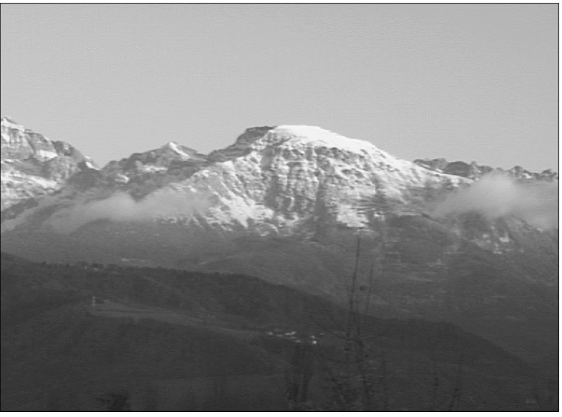
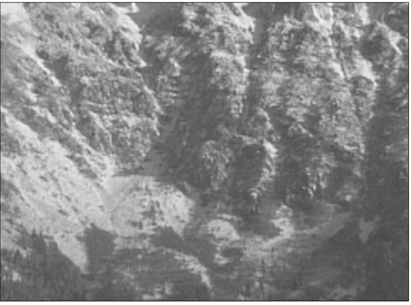
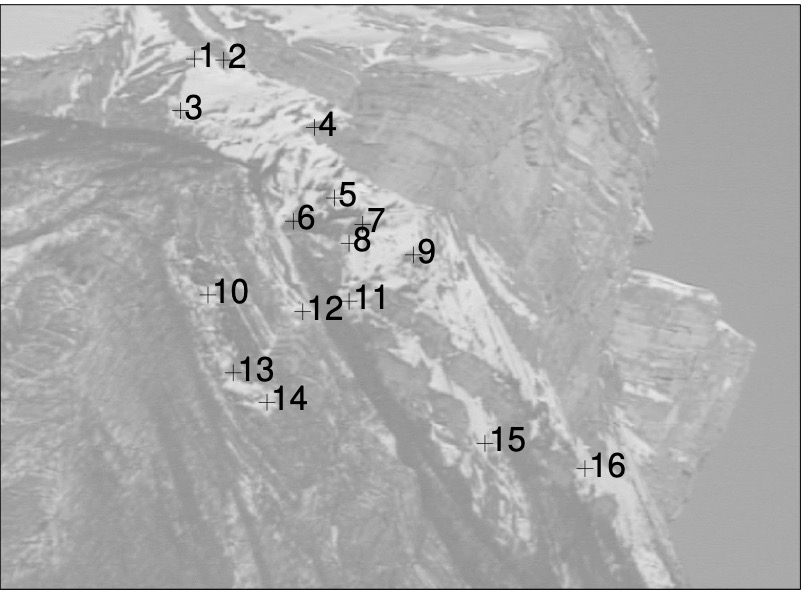
As an example we consider the image pair in Figure 1. Both images were taken with a camera placed at 11 kilometers (6.9 miles) away from the top of the mountain. For the first image (left) we used a focal length equal to 12mm while for the second one (right) we used a focal length equal to 72mm. Notice that the high-resolution image corresponds to a small region of the low-resolution one and it is quite difficult to find the exact position and size of this region. Moreover, the low-resolution image (left) covers in practice a wide range of resolutions because scene objects appear at various depths values.

Therefore, the search space associated with the feature-to-feature matching of two such images is larger and more complex than the one associated with the classical stereo matching paradigm. The classical approach to image matching proceeds as follows: (i) extract interesting point-features from each image, (ii) match them based on cross-correlation, (iii) compute the epipolar geometry through the robust estimation of the fundamental matrix, and (iv) establish many other matches once this matrix is known. For a number of reasons, this method cannot be applied to the problem at hand:

1. Point-feature extraction and matching are resolution-dependent processes.

2. The high-resolution image corresponds to a small region of the low-resolution one and hence the latter contains many features which do not have a match in the former.

3. It may be difficult to estimate the epipolar geometry because there is not enough depth associated with both the high resolution image and its associated small area of the low-resolution image.

The solution suggested in this paper consists of considering a scale-space representation of the high-resolution image and of matching the low-resolution image against the scale-space descriptions of the high-resolution one. A scale-space representation may be obtained by smoothing an image with Gaussian kernels of increasing standard deviations. Therefore, the high-resolution image will be described by a discrete set of images at various scales. On the premise that decreasing the resolution can be modeled as image smoothing which is equivalent to a scale change, the one-to-one image matching problem at hand becomes a one-to-many image matching problem [4].

In this paper we describe such a matching method. Key to its success are the following characteristics:

• The scale-space representation of image point features (or interest points) together with their associated descriptors;

• A geometric model describing the mapping from the high-resolution image to a region of the low-resolution one.

• An image-matching strategy combining point-to-point assignments with a robust estimation of the geometric mapping between image regions.

Several authors addressed the problem of matching two images gathered from two very different viewpoints [6, 20, 24, 25] but they did not consider a large change in resolution. The use of scale-space in conjunction with stereo matching has been restricted to hierarchical matching: correspondences obtained at low resolution constrain the search space at higher resolutions [7, 21, 14]. Scale-space properties are thoroughly studied in [15] and the same author attempted to characterize the best scale at which an image feature should be represented [16]. A similar idea is presented in [17] to detect stable points in scale space.

Our work is closely related to [9] who attempts to match two images of the same object gathered with two different zoom settings. Point-to-point correspondences are characterized in scale space by correlation traces. The method is able to recover the scale factor for which two image points are the most similar but it cannot deal with camera motions.

Local descriptors that are invariant with respect to affine grey value changes, image rotations, and image translations were studied theoretically in [13] and were used in the context of image matching in [22]. These descriptors are based on convolutions with Gaussian kernels and their derivatives. Therefore they are consistent with scale-space representations. They are best applied at image locations found by interest points and a recent study showed that the Harris corner detector [10] is the most reliable interest point detector [23]. However, these local descriptors are not scale-invariant and, in spite of good theoretical models for scale-space invariants [12, 15], it is more judicious, from a practical point of view, to compute local descriptors at various scales in a discrete scale-space [22].

The main contributions of this paper are the followings. We thoroughly study the behaviour of the Harris interest point detector under a similarity transformation. This detector comprises convolutions with two Gaussian kernels, one for weigthing and one for computing grey-level derivatives. We show under which conditions the detector is invariant to rotations and translations in the image plane. Based on this we derive a scale-space representation of interest points. This representation allows to match points from images at very different resolutions, which has never been performed in the past – up to a factor of 6. In order to match points we describe a way to represent local collections of points and we seek similarities between such local collections at different scales. Finally a one-to-many image matching technique (with scale adjustment) is described. Many examples with various scenes, camera configurations and settings illustrate the method both quantitatively and qualitatively.

Paper organization

The remainder of this paper is organized as follows. Section 2 briefly outlines the geometric model associated with the image pair. Section 3 suggests a framework for adapting the detection of interest points to scale changes, image rotations, and image translations. Section 4 describes the high-resolution to low-resolution matching and section 5 presents experimental results.

2 Geometric modeling

One of the key observations enabling the matching of two images at two different resolutions is that the high-resolution image corresponds to a small region of the low-resolution one. Without loss of generality, it may be assumed that the high-resolution image has homogeneous resolution because the observed 3-D features are, approximatively at the same distance. Clearly this is not the case for the low resolution image which contains various features at various ranges. The matching task therefore consists in finding a small region in the low resolution image that can be assigned to the whole high resolution one.

One reasonable assumption is to consider that the mapping between the high resolution image and the corresponding low-resolution region is a plane projective transformation, i.e., the scene corresponding to this region is planar. Such a homography may well be represented by a 3$\times$3 homogeneous full rank matrix H. Let $m$ be a point in the high-resolution image $I$ and $\mbox{\boldmath$m$}^{\prime}$ be a point in the low-resolution image $I^{\prime}$. One can characterize a region in the low-resolution image such that the points $m^{\prime}\in{\cal R}$ within this region verify:

$$\mbox{\boldmath$m$}^{\prime}\simeq\mbox{\bf H}\mbox{\boldmath$m$}$$ (1)

Similarly, points outside this region do not verify this equation. In general, image descriptors which are invariant to such a general plane-to-plane projective transformation are difficult to compute and therefore it is difficult to properly select potential candidate points satisfying eq. (1).

We can further simplify the geometric model and consider a restricted class of homographies, namely a rotation about the optical axis by an angle $\theta$, a translation in the image plane by a vector $(a,b)$, and a similitude factor  $h$:

$$\mbox{\boldmath$m$}^{\prime}=\left[\begin{array}[]{ccc}h\cos\theta&-h\sin\theta&a\\ h\sin\theta&h\cos\theta&b\\ 0&0&1\end{array}\right]\mbox{\boldmath$m$}$$ (2)

Notice that the projective equality in eq. (1) is replaced by an equality. In practice it will be useful to replace the 3-vectors $m$ and $\mbox{\boldmath$m$}^{\prime}$ used above by 2-vectors $x$ and $\mbox{\boldmath$x$}^{\prime}$ such that:

$$\mbox{\boldmath$m$}^{\prime}=\left(\begin{array}[]{c}u^{\prime}\\ v^{\prime}\\ 1\end{array}\right)=\left(\begin{array}[]{c}\mbox{\boldmath$x$}^{\prime}\\ 1\end{array}\right)\mbox{ and }\mbox{\boldmath$m$}=\left(\begin{array}[]{c}u\\ v\\ 1\end{array}\right)=\left(\begin{array}[]{c}\mbox{\boldmath$x$}\\ 1\end{array}\right)$$

With this notation, eq. (2) becomes:

$$\mbox{\boldmath$x$}^{\prime}=h\mbox{\bf R}\mbox{\boldmath$x$}+\mbox{\boldmath$t$}$$ (3)

where R is the 2$\times$2 rotation matrix and $t$ is the translation vector.

In order to match two images which differ by such a geometric transformation, one has to define a measure of similarity. One possibility is to use correlation. In this case, the similarity between $\mbox{\boldmath$x$}\in I$ and $\mbox{\boldmath$x$}^{\prime}\in I^{\prime}$ can be written as:

$$\sum_{\Delta\mbox{\boldmath$p$}}\left[I^{\prime}(\mbox{\boldmath$x$}^{\prime}-\Delta\mbox{\boldmath$p$}^{\prime})-I(\mbox{\boldmath$x$}-\Delta\mbox{\boldmath$p$})\right]^{2}$$

where $\Delta\mbox{\boldmath$p$}$ and $\Delta\mbox{\boldmath$p$}^{\prime}$ are shift vectors. With the substitution for $\mbox{\boldmath$x$}^{\prime}$ above, i.e., eq. (3) and with $\Delta\mbox{\boldmath$p$}^{\prime}=h\mbox{\bf R}\Delta\mbox{\boldmath$p$}$ we obtain:

$$\sum_{\Delta\mbox{\boldmath$p$}}\left[I^{\prime}(h\mbox{\bf R}(\mbox{\boldmath$x$}-\Delta\mbox{\boldmath$p$})+\mbox{\boldmath$t$})-I(\mbox{\boldmath$x$}-\Delta\mbox{\boldmath$p$})\right]^{2}$$ (4)

Therefore, one must find a scale factor $h$, a rotation matrix R, and a translation vector $t$ for which the expression above is minimized. The search space associated with such a technique is very large and the associated non-linear minimization procedure has to deal with a four-parameter cost function [8].

3 Interest point detection for image matching

Alternatively, one may use interest points. Ideally, one would like to characterize such image points by descriptors invariant to image rotation, translation and scale. Unfortunately, scale-invariant image descriptors are hard to compute in practice. Therefore, the matching strategy will build a discrete scale-space for the high-resolution image thus by-passing the scale-invariance problem. The image matching problem at hand then becomes a one-to-many image matching technique.

The steps for image-to-image matching are:

• extract sets of interest points from the two images, $(\mbox{\boldmath$x$}_{1},\ldots,\mbox{\boldmath$x$}_{M})$ and $(\mbox{\boldmath$x$}^{\prime}_{1},\ldots,\mbox{\boldmath$x$}^{\prime}_{N})$,

• characterize these points such that point-to-point comparisons are made possible, and

• determine the largest set of such correspondences compatible with a similarity between the high-resolution image and a low-resolution region.

The one-to-many matching algorithm uses this procedure and the image pair with the highest matching score determines the appropriate scale for matching and allows to estimate the scale change. The advantage of this approach mainly resides in step (iii) above. Two point-to-point correspondences are sufficient to estimate the similarity parameters described in eq. (2) (four such correspondences are necessary for a full homography) and therefore the largest set of point correspondences is found by an efficient robust estimator.

3.1 Interest point detection under similarity

We use the interest point detector proposed in [10]. This operator was studied experimentally and it was shown to be robust to image rotations, translations and illumination changes [23]. However, the Harris point detector is not invariant to changes in scale. In this section and in the next section we derive an exact formula for analyzing the behaviour of this interest-point detector over changes in scale, rotation, and translation.

We consider as before two images $I(\mbox{\boldmath$x$})$ and $I^{\prime}(\mbox{\boldmath$x$}^{\prime})$ with $\mbox{\boldmath$x$}=(u,v)^{\top}$ and $\mbox{\boldmath$x$}^{\prime}=(u^{\prime},v^{\prime})^{\top}$.

An interest point is detected in image $I$ (or in image $I^{\prime}$) as follows:

1. Compute the image derivatives in the $u$ and $v$ directions, $I_{u}$, and $I_{v}$. These computations are carried out by convolution with the differential of a Gaussian kernel of standard deviation $\sigma$:

   $$I_{u}(\mbox{\boldmath$x$},\sigma) = I(\mbox{\boldmath$x$})\star G_{u}(\mbox{\boldmath$x$},\sigma)$$

   $$I_{v}(\mbox{\boldmath$x$},\sigma) = I(\mbox{\boldmath$x$})\star G_{v}(\mbox{\boldmath$x$},\sigma)$$

   $$I_{u}I_{v}(\mbox{\boldmath$x$},\sigma) = I_{u}(\mbox{\boldmath$x$},\sigma)\,I_{v}(\mbox{\boldmath$x$},\sigma)$$

2. Form the auto-correlation matrix $\mbox{\bf M}(\mbox{\boldmath$x$},\sigma,\tilde{\sigma})$. This matrix sums up derivatives in a window around a point $x$ with a Gaussian kernel $G(\mbox{\boldmath$x$},\tilde{\sigma})$ being used for weighting:

   $$\mbox{\bf M}(\mbox{\boldmath$x$},\sigma,\tilde{\sigma})=\\ \left[\begin{array}[]{ll}G(\mbox{\boldmath$x$},\tilde{\sigma})\star I_{u}^{2}(\mbox{\boldmath$x$},\sigma)&G(\mbox{\boldmath$x$},\tilde{\sigma})\star I_{u}I_{v}(\mbox{\boldmath$x$},\sigma)\\ G(\mbox{\boldmath$x$},\tilde{\sigma})\star I_{u}I_{v}(\mbox{\boldmath$x$},\sigma)&G(\mbox{\boldmath$x$},\tilde{\sigma})\star I_{v}^{2}(\mbox{\boldmath$x$},\sigma)\end{array}\right]$$ (5)

3. $x$ is an interest point if the matrix M has two significant eigenvalues, that is, if the determinant and trace of this matrix verify a measure of “cornerness”:

   $${\cal C}(\mbox{\boldmath$x$})=\det(\mbox{\bf M}(\mbox{\boldmath$x$}))-\alpha\,\mbox{trace}\>(\mbox{\bf M}(\mbox{\boldmath$x$}))^{2}$$ (6)

   where $\alpha$ is a fixed parameter. An interest point is detected at image location $x$ if ${\cal C}(\mbox{\boldmath$x$})>t$, where $t$ is a threshold.

In order to study the behaviour of this operator to changes in scale, rotation, and translation, let us introduce the following notation:

$$\mbox{\bf M}(\mbox{\boldmath$x$},\sigma,\tilde{\sigma})=G(\mbox{\boldmath$x$},\tilde{\sigma})\star\mbox{\bf Q}(\mbox{\boldmath$x$},\sigma)$$ (7)

with:

$$\mbox{\bf Q}(\mbox{\boldmath$x$},\sigma)=\left[\begin{array}[]{ll}I_{u}^{2}(\mbox{\boldmath$x$},\sigma)&I_{u}I_{v}(\mbox{\boldmath$x$},\sigma)\\ I_{u}I_{v}(\mbox{\boldmath$x$},\sigma)&I_{v}^{2}(\mbox{\boldmath$x$},\sigma)\end{array}\right]=\left(\begin{array}[]{c}I_{u}\\ I_{v}\end{array}\right)\left(\begin{array}[]{cc}I_{u}&I_{v}\end{array}\right)$$ (8)

Under the assumption that the two images are properly normalized, the condition that must be satisfied is the equality of the two image intensities at two pixels:

$$I^{\prime}(\mbox{\boldmath$x$}^{\prime})=I(\mbox{\boldmath$x$})$$ (9)

This allows us to build a relationship that must hold between the autocorrelation matrices associated with two matching points in the two images and between cornerness measurements $\cal{C}$ and $\cal{C}^{\prime}$ associated with the autocorrelation matrix. The following proposition establishes these relationships:

Proposition 1

The auto-correlation matrices at locations $x$ (in image $I$) and $\mbox{\boldmath$x$}^{\prime}$ (in image $I^{\prime}$) are related by the following formula provided that the standard deviation of the smoothing Gaussian kernels are choosen such that $\tilde{\sigma}^{\prime}=h\tilde{\sigma}$:

$$\mbox{\bf M}^{\prime}(\mbox{\boldmath$x$}^{\prime},\sigma^{\prime},\tilde{\sigma}^{\prime})=\frac{1}{h^{2}}\mbox{\bf R}\mbox{\bf M}(\mbox{\boldmath$x$},\sigma,\tilde{\sigma})\mbox{\bf R}^{\top}$$ (10)

The equivalent relationship between the two cornerness measurements is given by the formula:

$${\cal C}^{\prime}=\frac{1}{h^{4}}{\cal C}$$ (11)

Proof: Noticing that the trace and determinant of a matrix are invariant with respect to a similarity transformation, i.e., $\mbox{\bf A}\rightarrow\mbox{\bf B}^{-1}\mbox{\bf A}\mbox{\bf B}$, it is straightforward to derive eq. (11) from eqs. (10) and (6).

In order to show that eq. (10) holds, let us derive both sides of eq. (9) with respect to $u$ and $v$:

$$\left(\begin{array}[]{c}I_{u}\\ I_{v}\end{array}\right)=\left(\begin{array}[]{c}\frac{\partial I}{\partial u}\\ \\ \frac{\partial I}{\partial v}\end{array}\right)=\left(\begin{array}[]{c}\frac{\partial I^{\prime}}{\partial u}\\ \\ \frac{\partial I^{\prime}}{\partial v}\end{array}\right)=\left(\begin{array}[]{c}I^{\prime}_{u}\\ I^{\prime}_{v}\end{array}\right)$$

The relationship between the pixel coordinates $\mbox{\boldmath$x$}^{\prime}=h\mbox{\bf R}\mbox{\boldmath$x$}+\mbox{\boldmath$t$}$ combined with the chain rule of derivation allows us to otbain:

$$\left(\begin{array}[]{c}I^{\prime}_{u}\\ I^{\prime}_{v}\end{array}\right)=\left[\begin{array}[]{cc}\frac{du^{\prime}}{du}&\frac{dv^{\prime}}{du}\\ &\\ \frac{du^{\prime}}{dv}&\frac{dv^{\prime}}{dv}\end{array}\right]\left(\begin{array}[]{c}I^{\prime}_{u^{\prime}}\\ I^{\prime}_{v^{\prime}}\end{array}\right)=h\mbox{\bf R}^{\top}\left(\begin{array}[]{c}I^{\prime}_{u^{\prime}}\\ I^{\prime}_{v^{\prime}}\end{array}\right)$$

The formulae above allow us to express a relationship between the quadratic forms $\mbox{\bf Q}(\mbox{\boldmath$x$},\sigma)$ and $\mbox{\bf Q}^{\prime}(\mbox{\boldmath$x$}^{\prime},\sigma^{\prime})$, i.e., eq. (8):

$$\mbox{\bf Q}(\mbox{\boldmath$x$},\sigma)=h^{2}\mbox{\bf R}^{\top}\mbox{\bf Q}^{\prime}(\mbox{\boldmath$x$}^{\prime},\sigma^{\prime})\mbox{\bf R}$$ (12)

Finally, using the properties of convolution applied to eq. (7) we obtain the formula given by eq. (10) (see appendix A for a formal derivation).

3.2 Interest point detection and scale-space

We consider now the scale-space associated with the high-resolution image $I$. The scale-space is obtained by convolving the initial image with a Gaussian kernel whose standard deviation is increasing monotonically, say $s\sigma$ with $s>1$. At scale $s$ we have the following image derivatives that allow the estimation of interest points:

$$I_{u}(\mbox{\boldmath$x$},s\sigma) = I(\mbox{\boldmath$x$})\star G_{u}(\mbox{\boldmath$x$},s\sigma)$$

$$I_{v}(\mbox{\boldmath$x$},s\sigma) = I(\mbox{\boldmath$x$})\star G_{v}(\mbox{\boldmath$x$},s\sigma)$$

If the task consists of matching a high-resolution image $I$ with a low-resolution one $I^{\prime}$, it is crucial to select the scale of $I$ at which this matching has to be performed. The scale parameter $s$ must “absorb” the similarity factor $h$ such that interest points that are detected in image $I$ at scale $s$ best correspond to interest points detected in image $I^{\prime}$. Since the resolution of $I$ decreases with increasing $s$ one needs to set:

$$s=\frac{1}{h}$$

The scale-space interest-point detector is then defined as follows. From eq. (10) and with the relationship between $s$ and $h$ we obtain the autocorrelation matrix:

$$\mbox{\bf M}_{s}(\mbox{\boldmath$x$},s\sigma,s\tilde{\sigma})=\\ s^{2}G(\mbox{\boldmath$x$},s\tilde{\sigma})\star\left[\begin{array}[]{cc}I_{u}^{2}(\mbox{\boldmath$x$},s\sigma)&I_{u}I_{v}(\mbox{\boldmath$x$},s\sigma)\\ I_{u}I_{v}(\mbox{\boldmath$x$},s\sigma)&I_{v}^{2}(\mbox{\boldmath$x$},s\sigma)\end{array}\right]$$ (13)

The cornerness measure becomes:

$${\cal C}_{s}(\mbox{\boldmath$x$})=s^{4}\left(\det(\mbox{\bf M}_{s}(\mbox{\boldmath$x$}))-\alpha\,\mbox{trace}\>(\mbox{\bf M}_{s}(\mbox{\boldmath$x$}))^{2}\right)$$

The following proposition is straightforward:

Proposition 2

If the interest points of an image $I$ are detected with the cornerness measurement ${\cal C}$ and with a threshold $t$ such that ${\cal C}>t$, then at scale $s$ the interest points are detected with $s^{4}{\cal C}_{s}>t$.

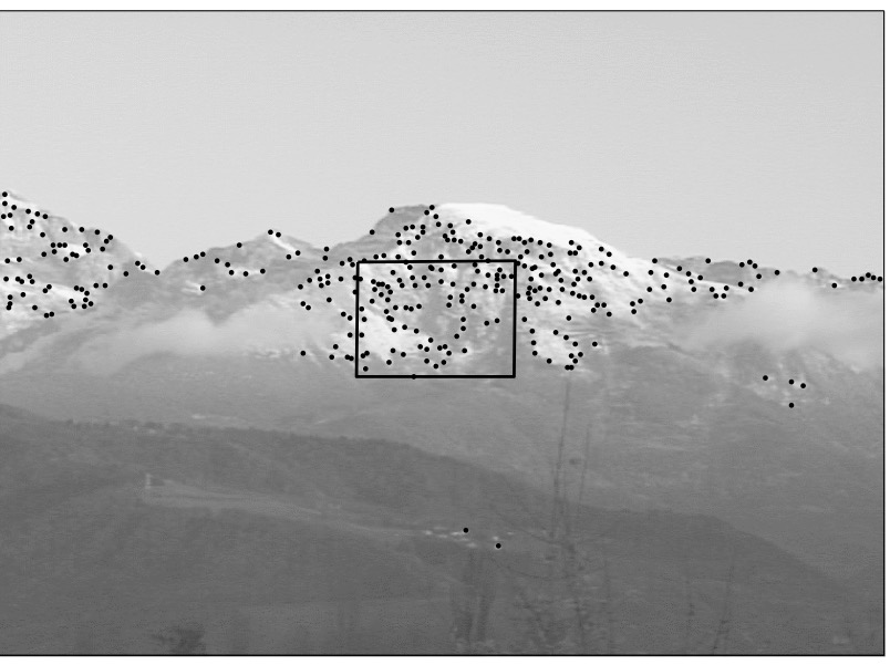
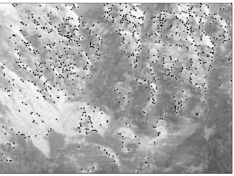
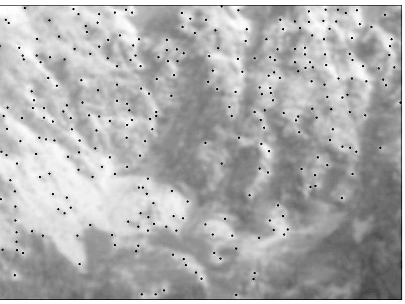
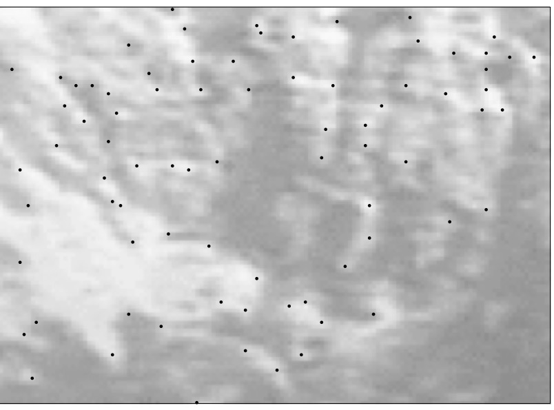
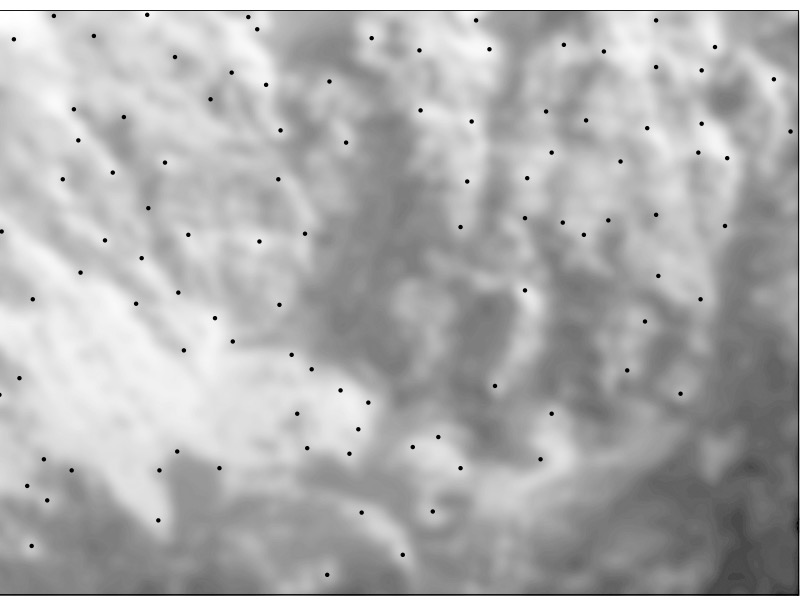
In order to illustrate the results obtained with this scale-space interest-point detector, we applied it to the high-resolution image of Figure 1 (right). Figure 2 shows these results with $\sigma=1$ and $\tilde{\sigma}=2$. The left side of this figure shows the interest points detected in the low-resolution image. The image region corresponding to the high resolution image is zoomed out by a factor of $5.3$ which is the true scale factor between the two images. The right side of this figure shows the high-resolution image with interest points detected at four different scales, 1, 3, 5, and 7. The best matching scale is shown, side by side, with the zoomed-out low-resolution region. This is clear evidence that the scale-space representation and detection of interest points facilitates the matching task.

$s=1$ $s=3$ $s=5$ $s=7$

Figure 2: Interest points detected at 4 scales (left) and the points detected in the corresponding low-resolution image (right).

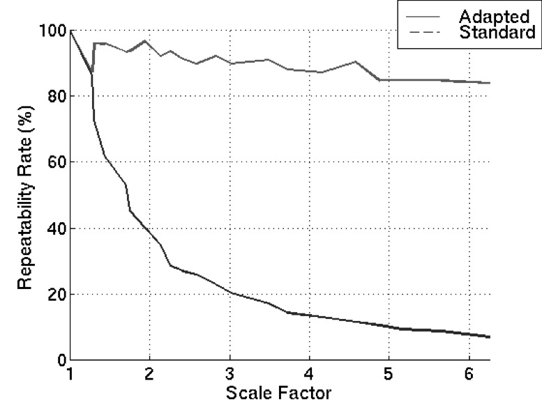
The importance of adapting the scale for interest point description and detection is shown on Figure 3. This figure shows a comparison between the standard Harris detector and the scale-space interest point detector. The scale factor varies from 1 to 6. The scale-space version uses the known scale factor between test images to adapt the interest point detection. The measure used in order to evaluate the performance is the repeatability rate introduced and thoroughly investigated in [23]. This measure takes into account the number of points repeated between the reference image and the scaled image with respect to the total number of points. One may clearly see that the scale-space detector shows very good performance. In the case of the standard detector the results are insufficient above a scale factor of 2 (less than 40% of the points are repeated).

Figure 3: Comparison of the standard Harris detector (Standard or bottom curve) and the scale-space version (Adapted or top curve). The comparison criteria is the repeatability rate which is displayed as a function of the scale factor.

4 Robust image matching

The scale-space extraction and representation of interest points will enable us to devise an image matching method. The main idea is to compare the low-resolution image at one scale with the high-resolution image at many scales. The scale at which the matching performs the best corresponds to the largest set of point-to-point assignments between a low-resolution image region and the high-resolution image.

Without loss of generality, while the low-resolution image $I^{\prime}$ is represented at one scale, the high-resolution image $I$ is represented at 8 different scales $\sigma$, 2$\sigma$, …, 8$\sigma$ with $\sigma=1$. At each scale $s_{i}$, interest points are extracted using eq. (13). Furthermore, each interest point (in both images and at all scales) is characterized by a description-vector whose elements are differential invariants. These invariants were introduced by Koenderink et al. [13] and were adapted for image matching by Schmid & Mohr [22].

Following Schmid & Mohr [22] two points of interest match if the Mahalanobis distance between their associated descriptors is small. Let $\mbox{\boldmath$V$}_{m}$ be a description-vector associated with point $m$. The distance between two points, $m$ and $m^{\prime}$ writes:

$$d_{\cal M}(m,m^{\prime})=\sqrt{(\mbox{\boldmath$V$}_{m}-\mbox{\boldmath$V$}_{m^{\prime}})^{\top}{\mathbf{\Lambda}}^{-1}(\mbox{\boldmath$V$}_{m}-\mbox{\boldmath$V$}_{m^{\prime}})}$$ (14)

This distance selects potentially good matches but is not powerful enough because it does not take into account neither local configurations of image points nor the global geometric transformation between the two images.

4.1 Matching based on local collections of points

One way to disambiguate point matches is to consider collections of interest points in a small image region and to try to match mutually compatible sets of points rather than individual points. Here compatibility is understood both in the sense of topology and geometry. The concept of mutually compatible feature matches stems from earlier work in 2-D object recognition [1], 3-D object recognition [2], [5], and stereo matching [11].

Here we are interested in considering a match $(m-m^{\prime})$, a neighbourhood $N(m)$ around point $m$, and a neighbourhood $N(m^{\prime})$ around $m^{\prime}$. We seek to establish whether there are other point matches within these two neighbourhoods which are topologically, photometrically, and geometrically compatible. Let $k$ be the number of point matches based on the Mahalanobis distance: $(m_{1}-m^{\prime}_{1})$, …$(m_{j}-m^{\prime}_{j})$, …$(m_{k}-m^{\prime}_{k})$, such that $m_{j}\in N(m)$, $m_{j}\neq m$ and $m^{\prime}_{j}\in N(m^{\prime})$, $m^{\prime}_{j}\neq m^{\prime}$ for all $j$, $1\leq j\leq k$.

These point-to-point matches allow to compute a similarity transformation between the two regions along the following lines:

1. select two matches (the central match plus an additional one),

2. compute the parameters of the associated similarity transformation, e.g. eq. (2),

3. verify how many other matches in the neighbourhood are consistent with these parameters,

4. etc.

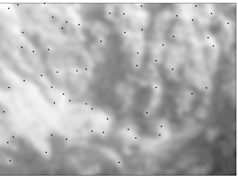
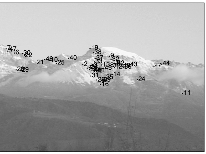
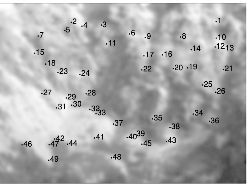
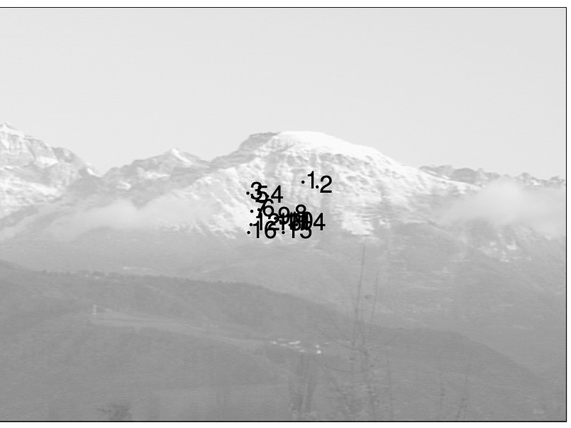
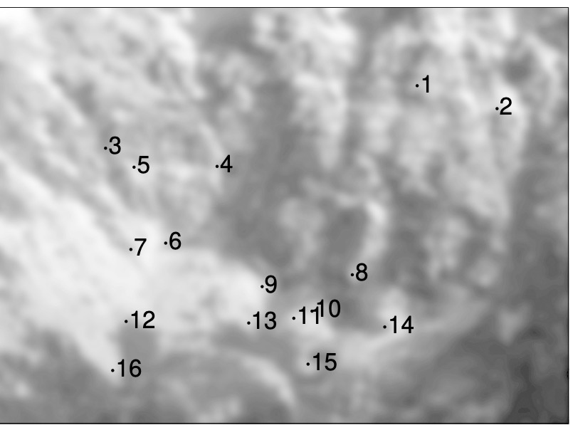
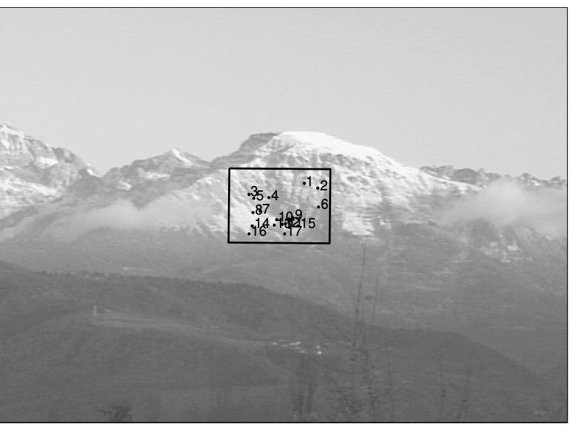
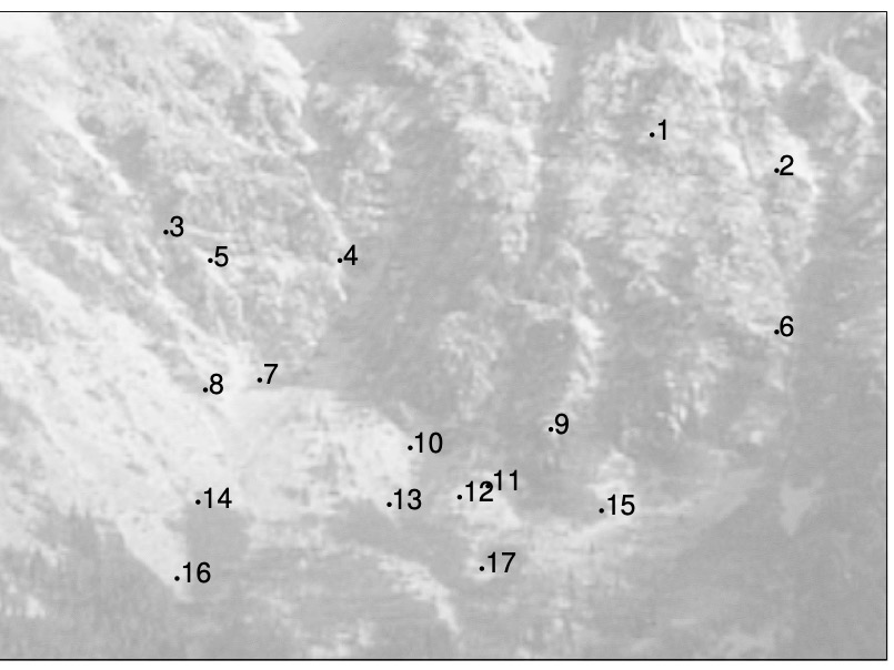
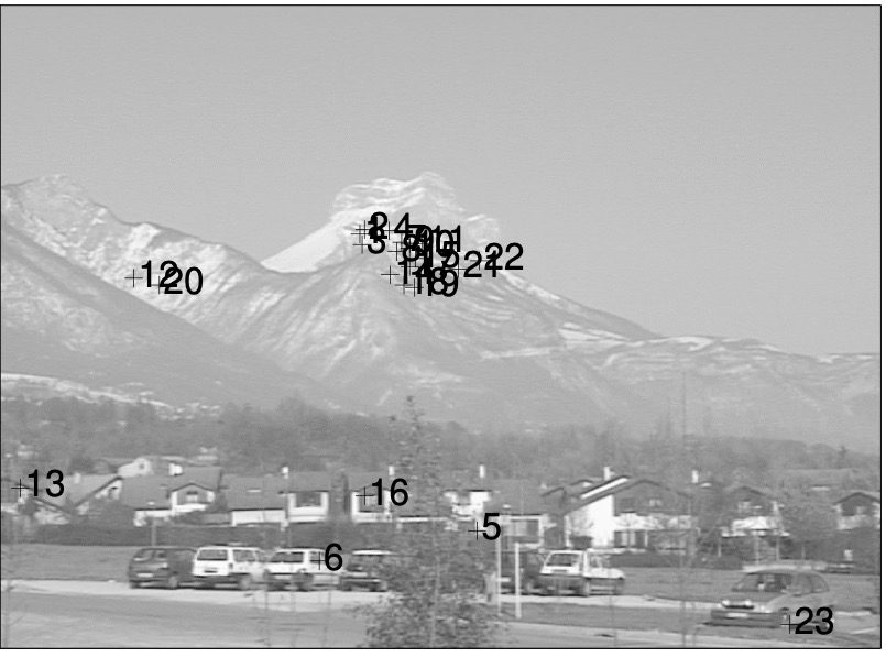
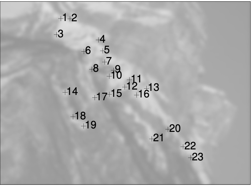
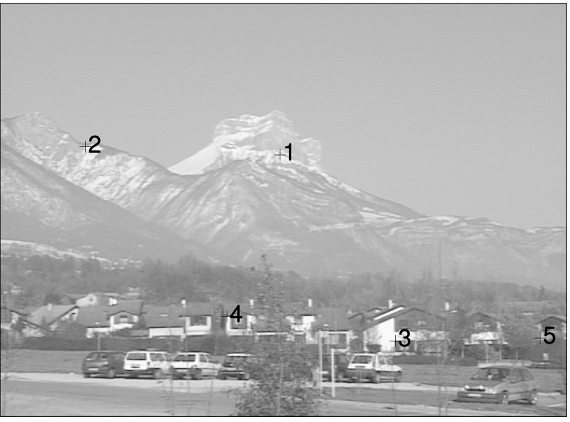
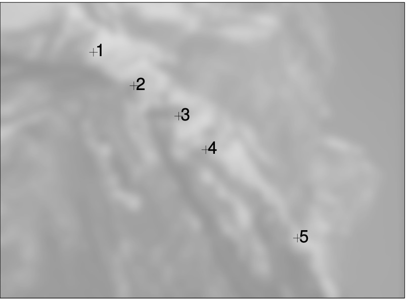
This matching method is implemented as a depth-first tree search. A final test based on eq. (4) allows to assess the match. The difference between matching points without local support and with local support is illustrated on figures 4 and 5. The image shown onto the left is the low-resolution image. The image shown onto the right is the high resolution image which is represented here at scale $5.3\sigma$ – the true scale factor between the two images. Figure 4 shows point matches established based on the Mahalanobis distance while Figure 5 shows the result of matching using the method just described.

Figure 4: Matching points using the Mahalanobis distance between their description vectors.

Figure 5: Matching points using constraints based on local collections of points.

Figure 6: Matching result for the image pair in Figure 1. The high-resolution image is mapped onto the low-resolution one using the similarity estimated from the 17 matches.

4.2 Matching at different scales

The matching algorithm considers, one by one, the scale-space representations of the high resolution image and attempts to find which one of these images best matches a region in the low resolution image. Since there is a strong relationship between scale and resolution, one may assume that the scale of the best match roughly corresponds to the resolution ratio between the two images. The final exact transformation between image and region is found by estimating the associated similarity.

Once an approximate scale has been selected using this strategy, a robust estimator takes as input the potential one-to-one point assignments, computes the best transformation between the two images, and splits the point assignments into two sets: (1) inliers, i.e., points lying within the small region corresponding to the similartity mapping of the high resolution image onto the low resolution one and (2) outliers, i.e., points that are either outside this region or mismatched points inside the region.

Commonly used robust estimators include M-estimators, least-median-squares (LMedS), and RANdom SAmple Consensus (RANSAC). In our case, the number of outliers may be quite large. This occurs in particular when the two images have very different resolutions and hence only 20% or less of the low-resolution image corresponds to the high resolution one. Therefore, we ruled out M-estimators because they tolerate only a few outliers. Among the two remaining techniques, we preferred RANSAC because it allows the user to define in advance the number of potential outliers through the selection of a threshold. Hence, this threshold can be chosen as a function of the scale factor. Details concerning threshold selection can be found in [3].

5 Experiments

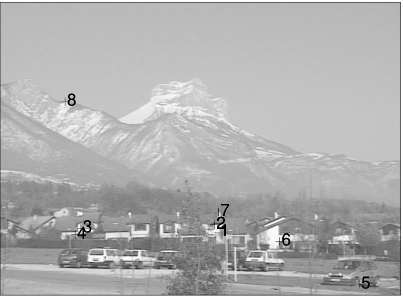
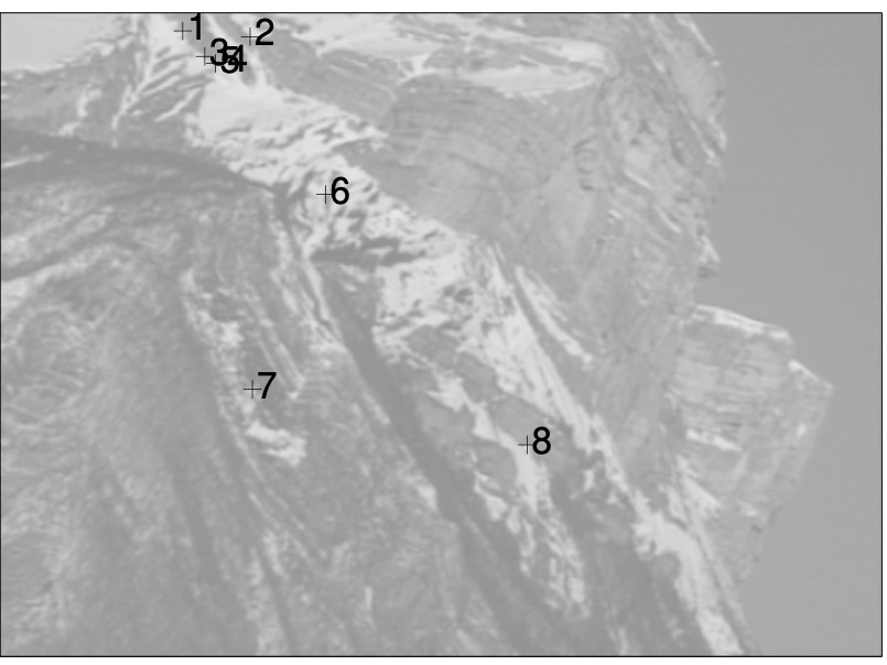
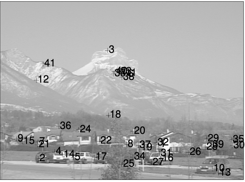
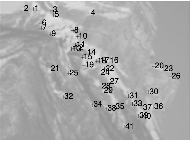
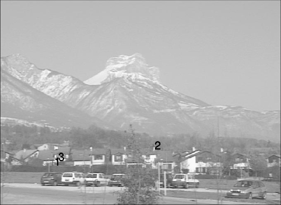
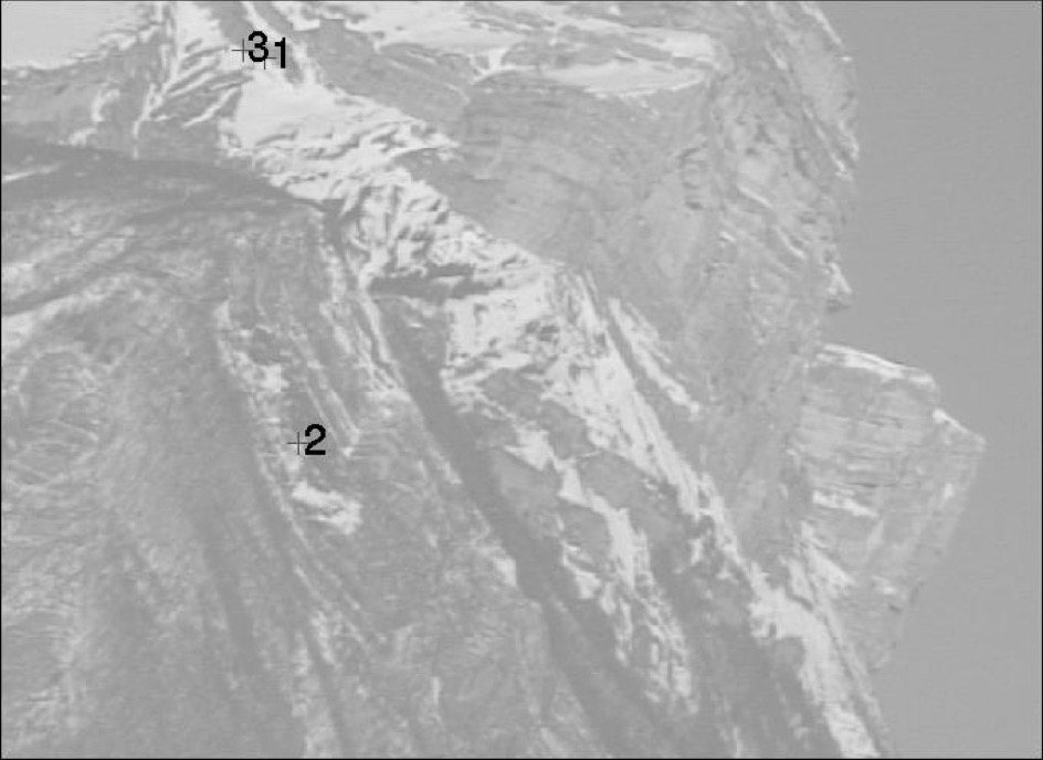
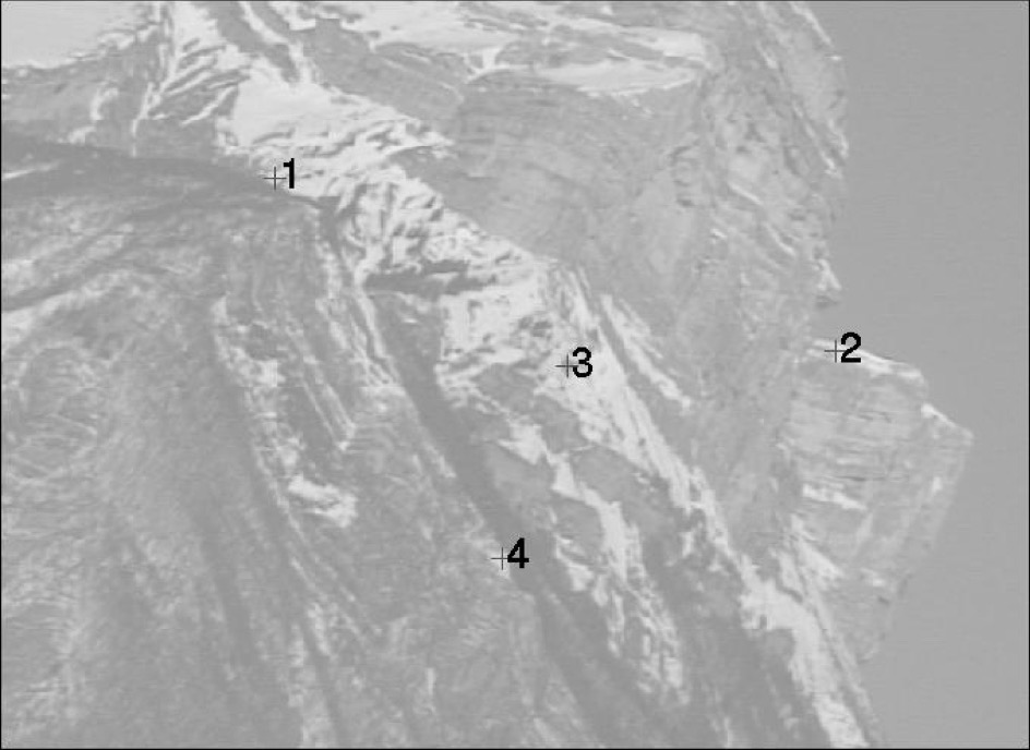
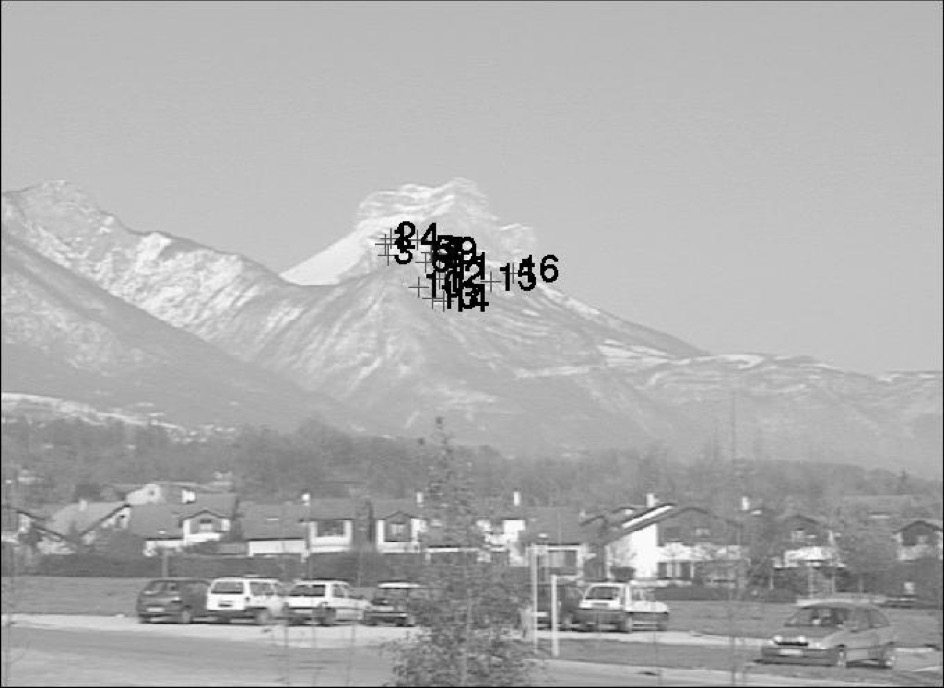
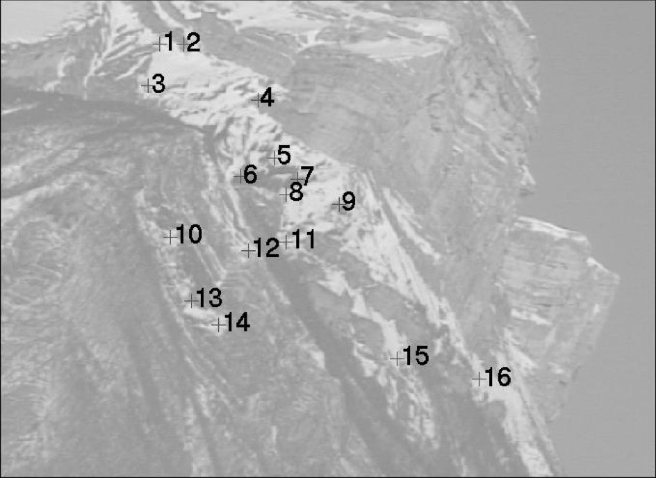
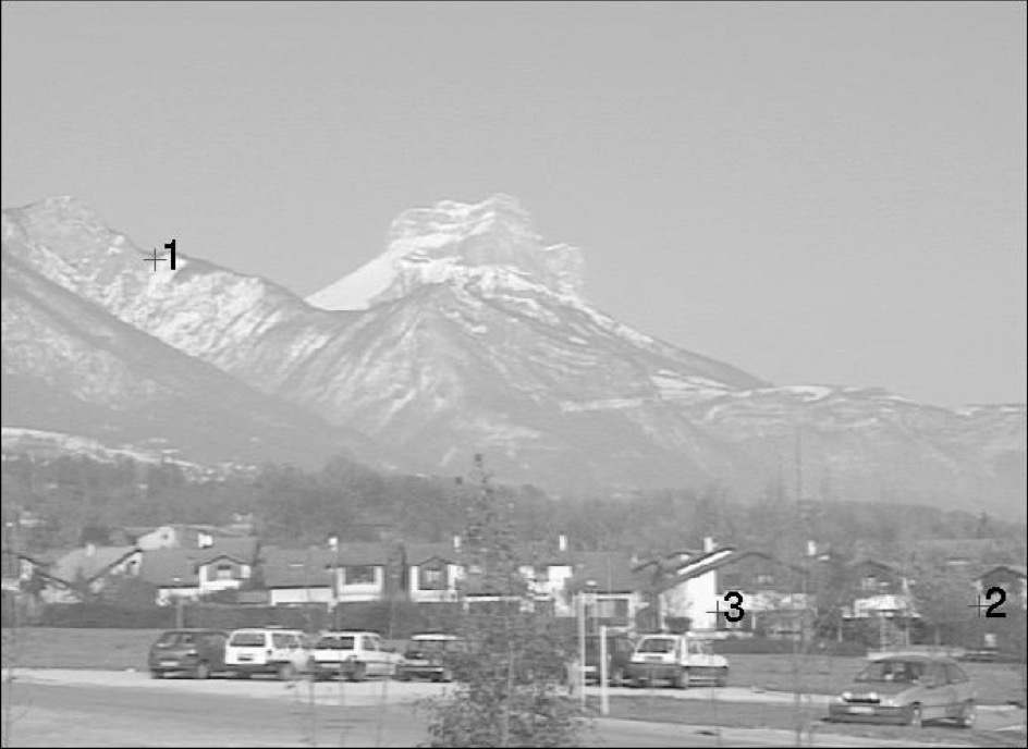
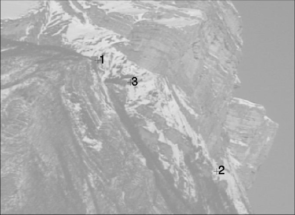
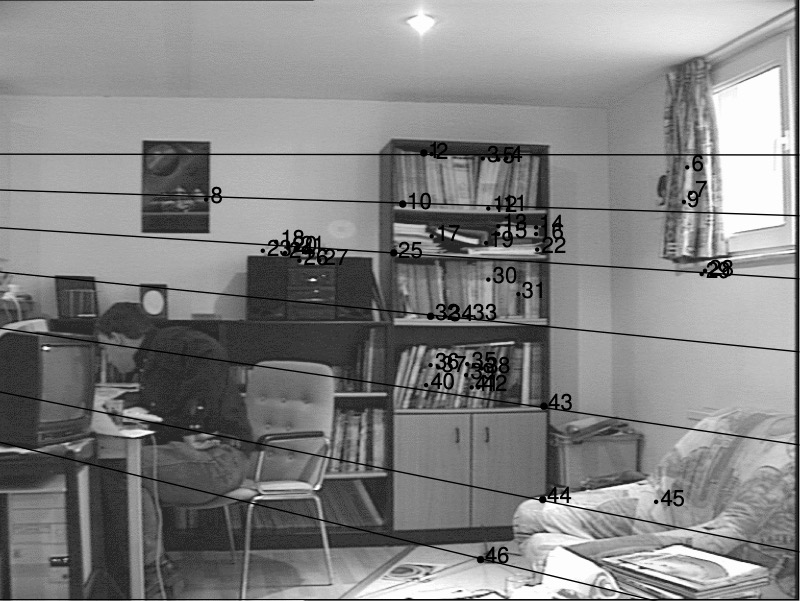
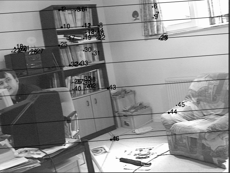
The matching strategy just described was applied and tested over a large number of image pairs where the resolution factor between the two images varied from 2 to 6. Let us explain in detail how this type of result is obtained for another example, e.g., Table 1 and Figures 7, 8, and 9. Interest points are first extracted from the low-resolution image at one scale ($s=1$) and from the high-resolution image at 8 different scales ($1$ to $8$). Therefore, eight image matchings are performed. Figure 7 shows the results of the point-to-point matching based on the Mahalanobis distance at four different scales: 1, 3, 5, and 8. These results correspond to the column named “Initial” in Table 1. Obviously, scales 3 and 5 have the best matches associated with them and scale 5 is a better candidate. Therefore, it would have been sufficient to run the remainder of the matching algorithm at scale 5 only. In practice we run the latter algorithm at all scales.

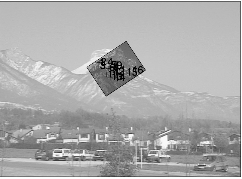
These initial matches are used for enforcing the local constraints and for the robust estimation of the similarity transformation. Figure 8 shows the results of applying both these two stages of the algorithm. The results are summarized in Table 1 in the column “Inliers”. One may verify that the best match is obtained at $s=5$. Out of 25 points detected at this scale, 23 among them have a potential assignment in the low-resolution image and 16 among them are finally selected by the robust matching technique. The latter rejected 30% of the matches. Notice that the resolution factor computed from the homography is correct for $s=4$, $s=5$ and $s=6$. Finally the image-to-region transformation thus obtained was applied to the high resolution image and this image is reproduced on top of the low-resolution one (cf. Figure 9).

Figure 7: Initial point-to-point assignments obtained at four scales (1,3,5,8). The true resolution factor between the two images is 5.

Figure 8: Inliers after applying the local constraints and the robust estimator to the previous results.

Figure 9: The final result obtained for the example in Figure 7. All of the 16 matches are correct. The high-resolution image is mapped onto the low-resolution one using the homography consistent with the 16 matches. The estimated rotation angle is 34 degrees and the estimated resolution change is 5.

Figure 10: Example for a 2D scene. All of the 11 matches are correct. The estimated rotation angle is 65 degrees and the estimated resolution change 3.7.

Figure 11: Example for the 3D scene “tunnel”. All of the 7 matches are correct. The estimated rotation angle is 77 degrees and the estimated resolution change is 3.2.

Figure 12: This figure shows the epipolar geometry as computed with the matching and estimation method described in this paper. Notice the large discrepancy in the viewpoints associated with the two images. The matcher seems to give advantage to collections of coplanar points.

Scale factor		No of points	No matches
$s$	estimated		initial	inliers	outliers
1	1.3	329	8	-	100 %
2	0.7	126	64	4	94 %
3	1.8	64	41	4	90 %
4	5	31	26	10	62 %
5	5	25	23	16	30 %
6	5	18	17	12	29 %
7	1.1	14	14	-	100 %
8	0.4	5	5	-	100 %

Table 1: This table shows, at each scale, the computed resolution factor, the number of points in the high-resolution image, the number of potential matches, the final number of matches, and the percentage of outliers. Notice that scales 4, 5 and 6 yield very similar results.

5.1 Further examples

So far we have been concerned with matching based on the hypothesis that there is a similarity transformation between one image and a region in the other image. This is a relatively restrictive hypothesis. The following examples show that the matching method described in this paper may well be applied (with some modifications) to cases were the two images differ by affine, projective, or epipolar transformations.

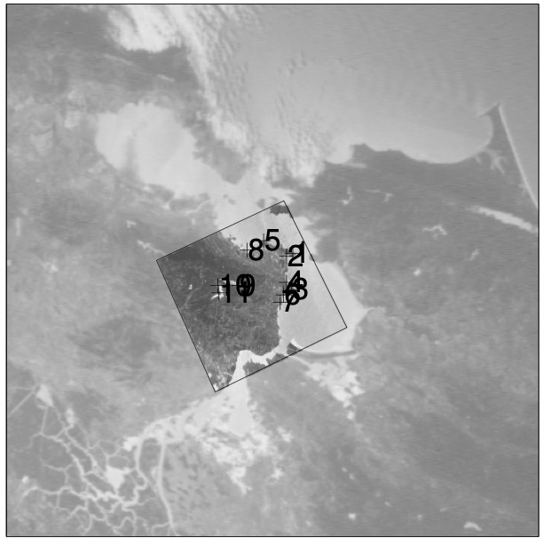
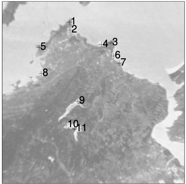
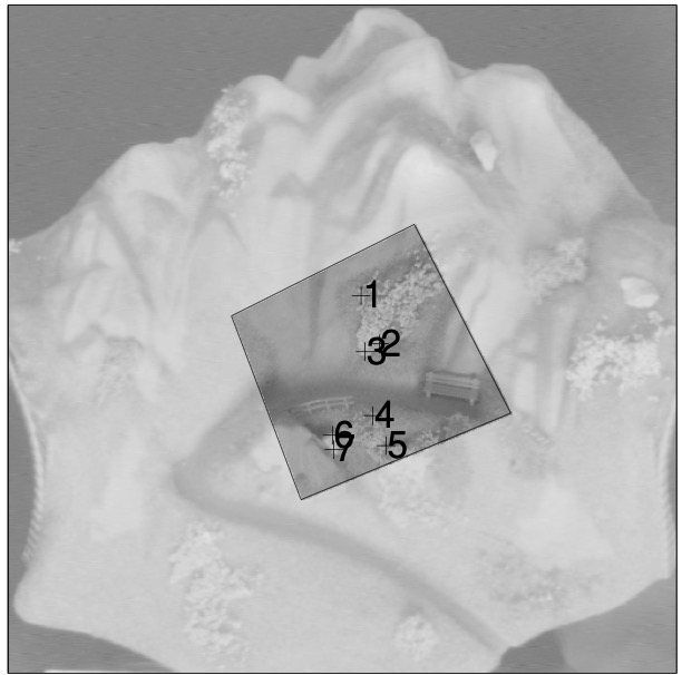
The matching strategy remains the same up to the robust estimator. The latter uses either an affine transformation, a plane homography, or the fundamental matrix to confirm matches and to reject outliers. Figure 10 shows an aerial view (left) as well as a detail (right). An affine transformation was hypothesized and correctly estimated. A second example (Figure 11) shows a mock-up, a planar detail, and the correct matches using a plane homography.

Figure 12 displays a stereo pair of a complex 3-D scene. The two images are taken from very different viewpoints with different zoom settings: Classical stereo matching methods fail to find the epipolar geometry. In spite of some mismatches along epipolar lines, the epipolar geometry is correctly estimated by the matching method described in this paper.

6 Conclusions

We presented a new method for matching images with two very different resolutions. We showed that it is enough to represent the high-resolution image in scale-space and we described a one-to-many robust image matching strategy. Key to the success of this method is the scale-space representation of interest points and their descriptors. We thoroughly investigated the similarity invariance of the Harris interest point detector as well as its scale-space behaviour. Recently this work was extended to characterize the most significant scale of an interest point and to devise a matching and indexing method that encapsulates scale changes [18]. The extension to affine-invariant local image descriptors is also on its way [19].

In spite of a huge number of publications in the image-matching domain, it seems to us that none of the existing methods is able to deal with large changes in resolution. Here we have been able to match images which differ by a resolution factor up to 6. In practice the images shown in this paper were gathered by varying the focal length using the zoom-lens of a digital camcorder. The advent of digital photography opens new fields of applications and we believe that our matching technique will allow the simultaneous exploitation of multiple viewpoints and variable resolutions.

Appendix A Interest point detection under similarity

In order to prove eq. (10) we consider the convolution of the Harris operator with a Gaussian kernel, i.e., eq. (7):

$$\mbox{\bf M}(\mbox{\boldmath$x$},\sigma,\tilde{\sigma})=G(\mbox{\boldmath$x$},\tilde{\sigma})\star\mbox{\bf Q}(\mbox{\boldmath$x$},\sigma)\\ =\int_{U}\int_{V}\mbox{\bf Q}(U,V)G(U-u,V-v,\tilde{\sigma})dUdV$$

Using eq. (12) we obtain:

$$G(\mbox{\boldmath$x$},\tilde{\sigma})\star\mbox{\bf Q}(\mbox{\boldmath$x$},\sigma)=\\ \int_{U}\int_{V}h^{2}\mbox{\bf R}^{\top}\mbox{\bf Q}^{\prime}(U^{\prime},V^{\prime})\mbox{\bf R}G(U-v,V-v,\tilde{\sigma})dUdV$$

The similarity transformation $\mbox{\boldmath$x$}^{\prime}=h\mbox{\bf R}\mbox{\boldmath$x$}+\mbox{\boldmath$t$}$ applied to vectors $(U\;V)^{\top}$ and $(u\;v)^{\top}$ yields:

$$dU^{\prime}dV^{\prime}=h^{2}dUdV$$

and

$$(U^{\prime}-u^{\prime})^{2}+(V^{\prime}-v^{\prime})^{2}=h^{2}((U-u)^{2}+(V-v)^{2})$$

Using the latter, the Gaussian kernel $G(U-u,V-v,\tilde{\sigma})$ becomes:

$$G(U-u,V-v,\tilde{\sigma}) =\frac{1}{2\pi\tilde{\sigma}^{2}}\exp\left(\frac{(U-u)^{2}+(V-v)^{2}}{2\tilde{\sigma}^{2}}\right)$$

$$=h^{2}\frac{1}{2\pi(h\tilde{\sigma})^{2}}\exp\left(\frac{(U^{\prime}-u^{\prime})^{2}+(V^{\prime}-v^{\prime})^{2}}{2(h\tilde{\sigma})^{2}}\right)$$

$$=h^{2}G(U^{\prime}-u^{\prime},V^{\prime}-v^{\prime},h\tilde{\sigma})$$

By substitution we get:

$$G(\tilde{\sigma})\star\mbox{\bf Q}(\mbox{\boldmath$x$},\sigma)=\\ h^{2}\mbox{\bf R}^{\top}\left(\int_{U^{\prime}}\int_{V^{\prime}}\mbox{\bf Q}^{\prime}(U^{\prime},V^{\prime})G(U^{\prime}-u^{\prime},V^{\prime}-v^{\prime},h\tilde{\sigma})dU^{\prime}dV^{\prime}\right)\mbox{\bf R}$$

By taking $\tilde{\sigma}^{\prime}=h\tilde{\sigma}$ we obtain:

$$G(\tilde{\sigma})\star\mbox{\bf Q}(\mbox{\boldmath$x$},\sigma)=h^{2}\mbox{\bf R}^{\top}\;G(\tilde{\sigma}^{\prime})\star\mbox{\bf Q}^{\prime}(\mbox{\boldmath$x$}^{\prime},\sigma^{\prime})\;\mbox{\bf R}$$

which proves the formula given by eq. (10).

References

- [1] R. C. Bolles and R. A. Cain. Recognizing and locating partially visible objects, the Local-Feature-Focus method. International Journal of Robotics Research, 1(3):57–82, 1982.
- [2] R. C. Bolles and R. Horaud. 3DPO: A three-dimensional part orientation system. International Journal of Robotics Research, 5(3):3–26, Fall 1986.
- [3] G. Csurka, D. Demirdjian, and R. Horaud. Finding the collineation between two projective reconstructions. Computer Vision and Image Understanding, 75(3):260–268, September 1999.
- [4] Y. Dufournaud, C. Schmid, and R. Horaud. Matching images with different resolutions. In IEEE Conference on Computer Vision and Pattern Recognition, pages 612–618, Hilton Head Island, SC, June 2000. IEEE Computer Society Press.
- [5] O.D. Faugeras and M. Hebert. The representation, recognition, and locating of 3-d objects. International Journal of Robotics Research, 5(3):27–52, Fall 1986.
- [6] N. Georgis, M. Petrou, and J. Kittler. On the correspondence problem for wide angular separation of non-coplanar points. Image and Vision Computing, 16:35–41, 1998.
- [7] F. Glazer, G. Reynolds, and P. Anandan. Scene matching by hierarchical correlation. In Proceedings of the Conference on Computer Vision and Pattern Recognition, Washington, DC, USA, pages 432–441, 1983.
- [8] A.W. Gruen. Adaptative least squares correlation: a powerful image matching technique. S. Afr. Journal of Photogrammetry, Remote Sensing and Cartography, 14(3):175–187, 1985.
- [9] B. B. Hansen and B. S. Morse. Multiscale image registration using scale trace correlation. In Proceedings of the Conference on Computer Vision and Pattern Recognition, Fort Collins, Colorado, USA, volume 2, pages 202–208, 1999.
- [10] C. Harris and M. Stephens. A combined corner and edge detector. In Alvey Vision Conference, pages 147–151, 1988.
- [11] R. Horaud and Th. Skordas. Stereo matching through feature grouping and maximal cliques. IEEE Transactions on Pattern Analysis and Machine Intelligence, PAMI-11(11):1168–1180, November 1989.
- [12] J.J. Koenderink. The structure of images. Biological Cybernetics, 50:363–396, 1984.
- [13] J.J. Koenderink and A.J. van Doorn. Representation of local geometry in the visual system. Biological Cybernetics, 55:367–375, 1987.
- [14] M. S. Lew and T. S. Huang. Optimal multi-scale matching. In Proceedings of the Conference on Computer Vision and Pattern Recognition, Fort Collins, Colorado, USA, volume 2, pages 88–93, June 1999.
- [15] T. Lindeberg. Scale-Space Theory in Computer Vision. Kluwer Academic Publishers, 1994.
- [16] T. Lindeberg. Feature detection with automatic scale selection. International Journal of Computer Vision, 30(2):79–116, 1998.
- [17] D. G. Lowe. Object recognition from local scale-invariant features. In Proceedings of the 7th International Conference on Computer Vision, Kerkyra, Greece, pages 1150–1157, 1999.
- [18] K. Mikolajczyk and C. Schmid. Indexing based on scale invariant interest points. In Proceedings of the 8th International Conference on Computer Vision, Vancouver, Canada, pages 525–531, 2001.
- [19] K. Mikolajczyk and C. Schmid. An affine invariant interest point detector. In Proceedings of the 7th European Conference on Computer Vision, Copenhagen, Denmark, volume I, pages 128–142, May 2002.
- [20] P. Pritchett and A. Zisserman. Wide baseline stereo matching. In Proceedings of the 6th International Conference on Computer Vision, Bombay, India, pages 754–760. ieee Computer Society Press, January 1998.
- [21] L. H. Quam. Hierarchical warp stereo. In Reading in computer Vision, pages 80–86. Morgan Kaufman, 1987.
- [22] C. Schmid and R. Mohr. Local grayvalue invariants for image retrieval. ieee Transactions on Pattern Analysis and Machine Intelligence, 19(5):530–534, May 1997.
- [23] C. Schmid, R. Mohr, and C. Bauckhage. Evaluation of interest point detectors. International Journal of Computer Vision, 37(2):151–172, 2000.
- [24] D. Tell and S. Carlsson. Wide baseline point matching using affine invariants computed from intensity profiles. In Proceedings of the 6th European Conference on Computer Vision, Dublin, Ireland, pages 814–828, 2000.
- [25] T. Tuytelaars, L. Van Gool, L. D’haene, and R. Koch. Matching of affinely invariant regions for visual servoing. In Proceedings of ieee International Conference on Robotics and Automation, pages 1601–1606, 1999.