Sparse decompositions of nonlinear dynamical systems and applications to moment-sum-of-squares relaxations

Abstract

In this paper we prove general sparse decomposition of dynamical systems provided that the vector field and constraint set possess certain structures, which we call subsystems. This notion is based on causal dependence in the dynamics between the different states. This results in sparse descriptions for three problems from nonlinear dynamical systems: region of attraction, maximum positively invariant set and (global) attractor. The decompositions can be paired with any method for computing (outer) approximations of these sets in order to reduce the computation to lower dimensional systems. We illustrate this by the methods from [15], [17] and [34] based on infinite-dimensional linear programming, as one example where the curse of dimensionality is present and hence dimension reduction is crucial. For polynomial dynamics, we show that these problems admit a sparse sum-of-squares (SOS) approximation with guaranteed convergence such that the number of variables in the largest SOS multiplier is given by the dimension of the largest subsystem appearing in the decomposition. The dimension of such subsystems depends on the sparse structure of the vector field and the constraint set and can allow for a significant reduction of the size of the semidefinite program (SDP) relaxations. The method is simple to use and based solely on convex optimization. Numerical examples demonstrate the approach.

,

1 Introduction

Many tasks concerning dynamical systems are of computationally complex nature and often not tractable in high dimension. Among these are the computations of the region of attraction (ROA), maximum positively invariant (MPI) set and global and weak attractors (GA and WA), all of which are the focus of this work. These sets are ubiquitous in the study of dynamical systems and have numerous applications. For example the ROA is the natural object to certify which initial values will be steered to a desired configuration after a finite time $T$ while the solution trajectory satisfies the state constraints at all times. The question of which initial values will stay in the constraint set for all positive times is answered by the MPI set. The GA describes which configurations will be reached uniformly by the solutions of the dynamical system asymptotically, while the WA describes the configurations that will be reached pointwise asymptotically. This is of importance for controlled systems with a given feedback control where one might be interested if the given feedback control forces the solution to converge to a specific point or whether a more complex limiting behavior may occur. Since these objects are complex in nature, computations of these are challenging tasks. Computational methods for the ROA have been pioneered by Zubov [43] in the 1960s and have a long history, summarized in [6]. A survey on the (controlled) MPI set and computational aspects can be found in [2]. Computations of the GA are typically approached via Lyapunov functions [10], via finite-time truncation or set oriented methods [8].

Given the curse of dimensionality problem present in computation of these sets, it is important to exploit structure in order to reduce the complexity. There are several concepts used for reducing the complexity, as for example symmetries (see, e.g., [9]) or knowledge of Lyapunov or Hamilton functions (see, e.g., [38]). Here we investigate a specific type of sparsity found in dynamical systems.

The central concept in this text is decoupling of the dynamical system into smaller subsystems. As subsystems we consider ensembles of states of the dynamical system that are causally independent from the remaining other states. This allows to treat these ensembles of states as separate dynamical systems. This results in computational time reduction and builds on the work [5]. Even though our main goal is to exploit this decoupling computationally, we study the sparse structure at a rather general level, allowing for our results to be used within other computational frameworks and for other problems than those encountered in this work. The main novelty is the following: (i) We generalize the method of [5] to far more general graph structures. (ii) We treat different problems than [5], namely additional to the ROA also the computation of the MPI set, GA and WA. (iii) We show that any method for approximating the ROA, the MPI set and GA with certain convergence properties allows a reduction to lower dimensional systems such that convergence is preserved. (iiii) As an example of such a procedure we use the proposed decoupling scheme within the moment sum-of-squares hierarchy framework, obtaining a sparse computational scheme for the ROA, MPI set and GA with a guaranteed convergence from the outside to the sets of interest; to the best of our knowledge this is the first time sparsity is exploited in the moment-sos hierarchy for dynamical systems without compromising convergence.

For the application to moment sum-of-squares framework we follow the approach from [15], [17] and [34] where outer approximations of the ROA, MPI set and GA are based on infinite dimensional linear programs on continuous functions approximated via the moment-sum-of-squares hierarchy (see [22] for a general introduction and  [14] for recent applications). Sparsity exploitation in static polynomial optimization goes back to the seminal work of [39], providing convergence results based on the so-called running intersection property. The situation in dynamical systems is more subtle and so far sparsity exploitation came at the cost of convergence such as in [36] where a different sparsity structure, not amenable to our techniques, was considered. Instead of exploiting correlation and term sparsity of the (static) polynomial optimization problem algebraically as in [39] or [41] we approach the problem from the perspective of the underlying dynamical system. This allows for a decoupling of the dynamical system into smaller subsystems while preserving convergence properties.

The framework proposed in this work (summarized in Algorithm 1) is general in nature and applicable to any method for approximating the ROA, MPI set or GA that satisfies certain convergence properties, as is the case, e.g., for the set-oriented methods for the GA [8].

To determine the subsystems we represent the interconnection between the dynamics of the states by the directed sparsity graph of the dynamics $f$ where the nodes are weighted by the dimension of the corresponding state space. We call a node $x_{j}$ an ancestor of another node $x_{i}$ if there exists a directed path from $x_{j}$ to $x_{i}$ in the (dimension weighted) sparsity graph of $f$. With this notation we can informally state our main result:

Theorem 1 (informal).

The dynamical system can be decomposed into subsystems where the largest dimension of these subsystems is determined by the largest weighted number of ancestors of one node in the dimension weighted sparsity graph of the dynamics. Further, this decomposition gives rise to decompositions of the ROA, MPI set, GA and WA.

This allows for a potentially dramatic reduction in computation time when the dynamics are very sparse in the sense considered in this work, i.e. when the sparsity graph allows a decoupling into (many) small subsystems.

We only consider continuous time dynamical systems in this paper but all the results hold in a similar fashion also for discrete time dynamical systems. Both the decoupling into subsystems and of the ROA, MPI and GA as well as the specific SOS approach have discrete time analogues.

2 Notations

The natural numbers are with zero included and denoted by $\mathbb{N}$. For a subset $J\subset\mathbb{N}$ we denote by $|J|$ its cardinality. The non-negative real numbers $[0,\infty)$ are denoted by $\mathbb{R}_{+}$. For two sets $K_{1},K_{2}$ we denote their symmetric difference given by $(K_{1}\setminus K_{2})\cup(K_{2}\setminus K_{1})$ by $K_{1}\Delta K_{2}$. The function $\mathrm{dist}(\cdot,K)$ denotes the distance function to $K$ and $\mathrm{dist}(K_{1},K_{2})$ denotes the Hausdorff distance of two subsets of $\mathbb{R}^{n}$ (with respect to a given metric or norm). The space of continuous functions on $X$ is denoted by $\mathcal{C}(X)$ and the space of continuously differentiable functions on $\mathbb{R}^{n}$ by $\mathcal{C}^{1}(\mathbb{R}^{n})$. The Lebesgue measure will always be denoted by $\lambda$. The ring of multivariate polynomials in variables $x=(x_{1},\ldots,x_{n})$ is denoted by $\mathbb{R}[x]=\mathbb{R}[x_{1},\ldots,x_{n}]$ and for $k\in\mathbb{N}$ the ring of multivariate polynomials of total degree at most $k$ is denoted by $\mathbb{R}[x]_{k}$. We will denote the open ball centered at the origin of radius $r$ with respect to the Euclidean metric by $B_{r}(0)$.

3 Setting and preliminary definitions

We consider a nonlinear dynamical system

$$\dot{x}=f(x)$$ (1)

with the state $x\in\mathbb{R}^{n}$ and a locally Lipschitz vector field $f:\mathbb{R}^{n}\to\mathbb{R}^{n}$. The following graph is a key tool in exploiting sparsity of $f$.

A central object in this text is the notion of subsystems of a dynamical system (1). We define a subsystem as follows.

Definition 1.

For a dynamical system $\dot{x}=f(x)$ on $\mathbb{R}^{n}$ we call a set of states $(x_{i})_{i\in I}$ for some index set $I\subset\{1,\ldots,n\}$ a subsystem of $\dot{x}=f(x)$ if we have

$$f_{I}\circ P_{I}=P_{I}\circ f$$ (2)

where $f_{I}:=(f_{i})_{i\in I}$ denotes the components of $f$ according to the index set $I$ and $P_{I}$ denotes the canonical projection onto the states $x_{I}$, i.e. $P_{I}(x):=x_{I}$.

If a set of states $(x_{i})_{i\in I}$ forms a subsystem we also say that the subsystem is induced by $I$. Since $f_{I}$ formally depends on $x\in\mathbb{R}^{n}$ we mean by the term $f_{I}\circ P_{I}$ that $f_{I}$ only depends on the variables $x_{I}$. If $\varphi_{t}$ denotes the flow of the dynamical system and $\varphi_{t}^{I}$ the flow of the subsystem, condition (2) translates to

$$\varphi_{t}^{I}\circ P_{I}=P_{I}\circ\varphi_{t}.$$ (3)

The equation in (3) states that the subsystems behave like factor systems, i.e. the projections map solutions of the whole system to solutions of the subsystems, and that we can view the dynamical system acting on the states indexed by $I$ independently from the remaining other states.

Remark 1.

The notion of a subsystem is closely related to the concept of causality ([13], [30], [29]). Namely, a set $I\subset\{1,\ldots,n\}$ induces a subsystem if and only if there is no causal influence on the states indexed by $I$, by the remaining states (not indexed by $I$).

The so-called (weighted) sparsity graph of the dynamics $f$ gives a discrete representation of the dependence between different states.

Definition 2.

Let the variable $x\in\mathbb{R}^{n}$ and the function $f:\mathbb{R}^{n}\to\mathbb{R}^{n}$ be partitioned (after a possible permutation of indices) as $x=(x_{1},\ldots,x_{N})$ and $f=(f_{1},\ldots,f_{N})$ with $x_{i}\in\mathbb{R}^{n_{i}}$, $f_{i}:\mathbb{R}^{n}\to\mathbb{R}^{n_{i}}$ and $\sum_{i=1}^{N}n_{i}=n$. The dimension weighted sparsity graph associated to $f$ induced by this partition is defined by:

1. The set of nodes is $(x_{1},\ldots,x_{N})$.

2. $(x_{i},x_{j})$ is an edge if the function $f_{j}$ depends on $x_{i}$ .

3. The weight of a node $x_{i}$ is equal to $n_{i}$.

Remark 2.

Without putting weights on nodes we call the graph just sparsity graph of $f$ (induced by the partitioning). The (dimension weighted) sparsity graph is not unique as it depends on the partition of $x$ and $f$. Choosing a good partition, i.e. a partition that that allows a decoupling into subsystems of small size as the partition from Lemma 2, is key to maximizing the computational savings obtained from the sparse SDP relaxations developed in this work in section 7.

Remark 3.

For a dynamical system a sparsity graph describes the dependence of the dynamics of a state on other states. More precisely, there exists a directed path from $i$ to $j$ in the sparsity graph of $f$ if and only if the dynamics of $x_{j}$ depend (indirectly via other states) on the state $x_{i}$.

As an example consider the function $f:\mathbb{R}^{10}\rightarrow\mathbb{R}^{10}$

$$f(y_{1},\ldots,y_{10}) = (y_{1}^{2}y_{2},y_{1}y_{2},y_{3}y_{2}+y_{3}^{2},y_{7}-y_{4}^{4},y_{1}y_{5}^{2},$$

$$y_{2}y_{6},y_{2}^{3}y_{6}y_{7},y_{3}^{2}y_{6}y_{8}^{2},y_{6}y_{9}^{5},y_{7}^{2}).$$

The grouping $x_{1}=(y_{1},y_{2})$, $x_{2}=y_{3}$, $x_{3}=(y_{4},y_{5})$, $x_{4}=(y_{6},y_{7})$ and $x_{5}=(y_{8},y_{9},y_{10})$ induces the functions $f_{1}(y_{1},y_{2})=(y_{1}^{2}y_{2},y_{1}y_{2}),f_{2}(y_{3})=(y_{3}y_{2}+y_{3}^{2}),f_{3}(y_{4},y_{5})=(y_{7}-y_{4}^{4},y_{7}y_{5}^{2}),f_{4}(y_{6},y_{7})=(y_{2}y_{6},y_{2}^{3}y_{6}y_{7})$ and $f_{5}(y_{8},y_{9},y_{10})=(y_{3}^{2}y_{6}y_{8}^{2},y_{6}y_{9}^{5},y_{7}^{2})$ according to Definition 2. Figure 2 shows its dimension weighted sparsity graph.

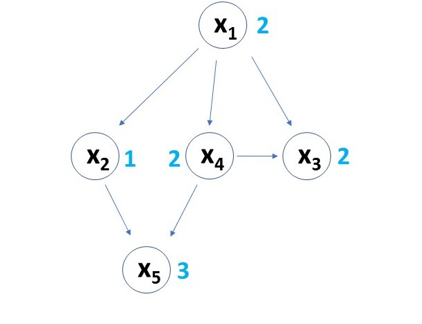
Figure 1: The dimension weighted sparsity graph of the function (3) with respect to the partitioning $x_{1}=(y_{1},y_{2})$, $x_{2}=y_{3}$, $x_{3}=(y_{4},y_{5})$, $x_{4}=(y_{6},y_{7},y_{8},y_{9})$ and $x_{5}=(y_{10},y_{11},y_{12})$

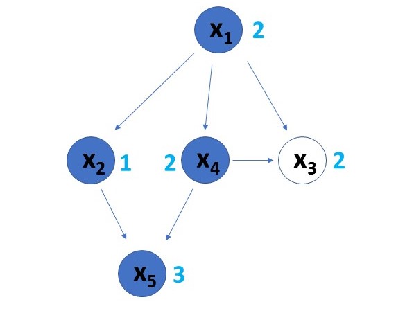
Figure 2: Past of $x_{5}$ in the sparsity graph from Figure 2

Definition 3 (Predecessor, leaf, Past).

1. For a sparsity graph we call a node $x_{i}$ a predecessor of node $x_{j}$ if either $x_{i}=x_{j}$ or if there is a directed path from $x_{i}$ to $x_{j}$.

2. A node $x_{i}$ is called a leaf if it does not have a successor (i.e., all nodes connected to $x_{i}$ are its predecessors).

3. The set of all predecessors of $x_{i}$ is called the past of $x_{i}$ and denoted by $\mathbf{P}(x_{i})$.

4. The largest dimension weighted past $\omega$ in a directed graph with weights $n_{i}$ and nodes $x_{i}$ is given by

   $$\omega:=\max\limits_{i}\sum\limits_{x_{j}\in\mathbf{P}(x_{i})}n_{j}.$$ (4)

For the graph from figure 2, the node $x_{5}$ has the largest weighted path. Its past is colored in blue in Figure 2.

In Remark 3 we have seen that the past of a node $x_{i}$ determines all the nodes the dynamics of $x_{i}$ (indirectly) depend on. Therefore the following definition is closely related to the notion of the past of a node.

For a given node $x_{i}$ the past $\mathbf{P}(x_{i})$ of this node determines the states of the smallest subsystem of the dynamical system containing $x_{i}$, and we refer to this subsystem as the subsystem induced by $\mathbf{P}(x_{i})$. In acyclic sparsity graphs the nodes with maximal past are leafs, i.e. nodes with no successor, because a successor has a larger past than its predecessor.

The sets related to dynamical systems we focus on in this text are the region of attraction, maxmimum positively invariant set and (global) attractors. We define these sets in the following.

Definition 4 (Region of attraction).

For a dynamical system, a finite time $T\in\mathbb{R}_{+}$ and a target set $X_{\mathrm{T}}\subset X$ the region of attraction (ROA) of $X_{\mathrm{T}}$ is defined as

$$R_{T}:=\big{\{}x_{0}\in X : \exists x(\cdot)\text{ s.t. }\dot{x}(t)=f(x(t)),\;x(0)=x_{0},$$ (5)

$$x(t)\in X\text{ on }[0,T],\;x(T)\in X_{\mathrm{T}}\big{\}}.$$

Remark 4.

The reachable set from an initial set $X_{\mathrm{I}}\subset X$ in time $T$

$$S_{T}:=\{x\in X : \dot{x}(t)=f(x(t)),x(t)\in X\text{ on }[0,T],$$ (6)

$$x(T)=x,x(0)\in X_{\mathrm{I}}\}$$

can be obtained by time reversal, i.e. by $S_{T}=R_{T}$ for $X_{\mathrm{T}}:=X_{\mathrm{I}}$ and the dynamics given by $\dot{x}=-f(x)$.

Definition 5 (Maximum positively invariant set).

For a dynamical system the maximum positively invariant (MPI) set is the set of initial conditions $x_{0}$ such that the solutions $\varphi_{t}(x_{0})$ stay in $X$ for all $t\in\mathbb{R}_{+}$.

The MPI set will be denoted by $M_{+}$ in the following.

Definition 6 (Global and weak attractor).

A compact set $\mathcal{A}\subset X$ is called

1. the global attractor (GA) if it is minimal uniformly attracting, i.e., it is the smallest compact set $\mathcal{A}$ such that

   $$\lim_{t\to\infty}\mathrm{dist}(\varphi_{t}(M_{+}),\mathcal{A})=0.$$

2. weak attractor if it is minimal pointwise attracting, i.e. it is the smallest compact set $\mathcal{A}_{w}$ such that for all $x\in M_{+}$

   $$\lim_{t\to\infty}\mathrm{dist}(\varphi_{t}(x),\mathcal{A}_{w})=0.$$

Remark 5.

An important property of the global attractor is that it is characterized by being invariant, i.e. $\varphi_{t}(\mathcal{A})=\mathcal{A}$ for all $t\in\mathbb{R}_{+}$, and attractive see [33].

4 Motivation for subsystems

In this section we provide several examples of systems from practice that possess the sparsity structure considered in our work. In Remark 1 we noted that subsystems are closely related to causality, highlighting an important connection between sparsity and causality. Further it indicates that systems with low causal interconnection provide examples of systems where sparsity in form of subsystems can be exploited.

Network systems

Causality describes the flow of information or the dependence between different states. From this we observe that social networks provide many important and complex examples were sparsity can be observed. This is expressed for instance in the so-called “social-bubbles” as well as the directed flow of information from some people (such as “influencers”, politicians, celebrities, etc.) to their “followers”. Other properties of social networks such as “locality” lead to subsystems as well. That is, interactions at many places take place physically which implies that geographical location influences the flow of information leading to flow of information along continent $\rightarrow$ country $\rightarrow$ department $\rightarrow$ city $\rightarrow$ family/company/school/social clubs etc. Due to the complexity (including its size) of social networks (exact) reduction techniques are necessary for understanding and analysis such networks with applications reaching from epidemologie, political influence, stability, etc. We give an example of a social network graph in 3. Further large scale networks that seem to exhibit subsystems are communication networks, interacting networks, hierarchical networks, citation networks, the internet, food web among others. Some of the mentioned examples are discussed in [35]. Another interesting class of systems where subsystems appear can be found in (distributed) mutlicellular programming [32], [37]. Another class of networks systems, where sparse structures can be found, are supply networks such as water networks, data routing and logistic networks [3] and traffic networks [23], [20]. Whenever there is no back-flow in the supply network, subsystems tend to appear.

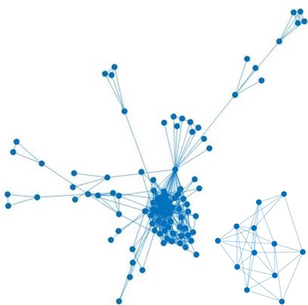
Figure 3: Example of a social network graph

Power grid

Another important example are power flow networks, in particular radial distribution networks [4] where energy is transported from a power plant to cities to districts/suburbs to streets to housing complexes to individual housing units as in Figure 4. An optimal control problem for radial distribution network is described in [25] and a dynamic programming approach with fewer variables, based on the sparse structure, was proposed. The system architecture of a radial distribution networks, that is, directed and branching flow (of energy) without cycles is the most direct extension of a prototype setting, that we will describe in the following Section 5. In fact, systems with a tree-structure with many branches are the most sparse systems (with respect to our notion of sparsity).

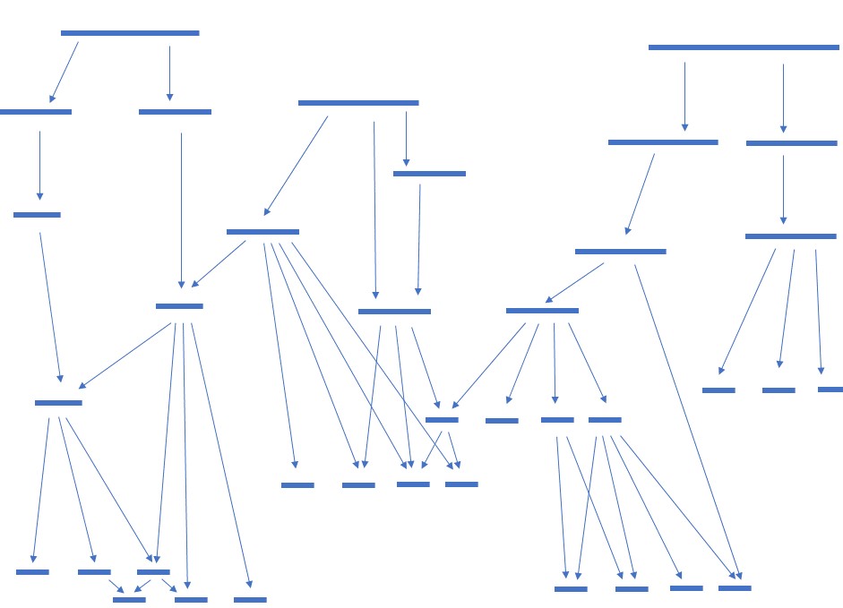
Figure 4: Example of a power grid

Chemical reactions

More generally, systems with information flowing only downstream are called cascaded systems. As mentioned they appear in power flows ([4], [27]) but also in water-energy cascade reservoir systems [24] or in chemical systems where products of reactions act as reactants or enzymes for further reactions downstream [42]. Examples of such are the Heinrich-Model, see Figure 5, and Huang-Ferrell model ([42]).

Figure 5: The Heinrich Model for a chemical cascade reaction where the product of one reaction acts as enzyme for the next reaction

In the case of the Heinrich-Model and Huang-Ferrell model the cascade does not have any branching. This is illustrated in the following Figure 6.

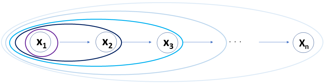
Figure 6: Cascade without branching. Circles around states indicate subsystems, i.e. the all subsystems are induced by index sets of the form $I=\{1,\ldots,k\}$ for $1\leq k\leq n$.

A structure as in Figure 6 means for our approach that we have to consider the whole system itself as a subsystem as well, and hence cannot decouple into subsystem of which all have strictly lower dimension than the whole system. Therefore the computational benefit in such cases is limited. Nevertheless, we do get further qualitative insight by investigating the lower dimensional subsystems according to Theorem 2.

Our work is based on [5] where a 6D Quadrotor was used to illustrate the application of sparsity to reachable set computation. Another example from robotics involving sparsity can be found in [1] where control of a monocycle robot is considered.

5 Sparse dynamics: the prototype setting

We illustrate the procedure at the basic example of a dynamical that allows a decomposition. Nevertheless this examples inspired this work, is studied in [5] and has the following form (with corresponding sparsity graph on the right)

$$\dot{x}_{1} = f_{1}(x_{1})$$

$$\dot{x}_{2} = f_{2}(x_{1},x_{2})$$ (7)

$$\dot{x}_{3} = f_{3}(x_{1},x_{3})$$

on the state space $\mathbb{R}^{n_{1}}\times\mathbb{R}^{n_{2}}\times\mathbb{R}^{n_{3}}$ and we consider a constraint set $X\subset\mathbb{R}^{n_{1}+n_{2}+n_{3}}$ and locally Lipschitz continuous functions $f_{1}:X\rightarrow\mathbb{R}^{n_{1}}$, $f_{2}:X\rightarrow\mathbb{R}^{n_{2}}$ and $f_{3}:X\rightarrow\mathbb{R}^{n_{3}}$ where $f_{1}$ only depends on $x_{1}$, i.e. is constant in $(x_{2},x_{3})$, $f_{2}$ only depends on $(x_{1},x_{2})$, i.e. is constant in $x_{3}$ and $f_{3}$ only depends on $(x_{1},x_{3})$, i.e. is constant in $x_{2}$. The sparsity graph of the system (5) has the “2–cherry” structure depicted in Figure 5. This indicates that the system splits into the decoupled dynamics

$$\frac{\mathrm{d}}{\mathrm{dt}}(x_{1},x_{2})=(f_{1},f_{2})(x_{1},x_{2})$$ (8)

with corresponding flow $\varphi_{t}^{2}$ and

$$\frac{\mathrm{d}}{\mathrm{dt}}(x_{1},x_{3})=(f_{1},f_{3})(x_{1},x_{3})$$ (9)

with corresponding flow $\varphi_{t}^{(3)}$ and

$$\dot{x}_{1}=f_{1}(x_{1})$$ (10)

with corresponding flow $\varphi_{t}^{(1)}$. Let $P_{\{1,i\}}$ denote the canonical projection onto $(x_{1},x_{i})$ and $P_{\{1\}}$ the canonical projection onto the $x_{1}$ component . Then the subsystem relations (8) and (9) read

$$(f_{1},f_{2})\circ P_{\{1,2\}}=P_{\{1,2\}}\circ f,(f_{1},f_{3})\circ P_{\{1,3\}}=P_{\{1,3\}}\circ f$$

as well as $f_{1}\circ P_{\{1\}}=P_{\{1\}}\circ f$ and we have for the corresponding flows

$$\varphi_{t}^{(i)}\circ P_{\{1,i\}}=P_{\{1,2\}}\circ\varphi_{t}\;,\;\varphi_{t}^{(1)}\circ P_{\{1\}}=P_{\{1\}}\circ\varphi_{t}$$ (11)

for $i=2,3$ and for all $t\in\mathbb{R}_{+}$. Note that the $x_{1}$-component of the flows $\varphi^{(2)}$ and $\varphi^{(3)}$ are given by $\varphi^{(1)}$ due to the decoupled dynamics of $x_{1}$.

The state constraints need to be taken into account more carefully. For instance the constraint set for (8) for a fixed $x_{3}$ is given by

$$X_{1,2}(x_{3}):=\{(x_{1},x_{2})\in\mathbb{R}^{n_{1}}\times\mathbb{R}^{n_{2}}:(x_{1},x_{2},x_{3})\in X\}.$$ (12)

In a similar way we define

$$X_{1,3}(x_{2}):=\{(x_{1},x_{3})\in\mathbb{R}^{n_{1}}\times\mathbb{R}^{n_{3}}:(x_{1},x_{2},x_{3})\in X\}.$$ (13)

and

$$X_{1}(x_{2},x_{3}):=\{x_{1}\in\mathbb{R}^{n_{1}}:(x_{1},x_{2},x_{3})\in X\}.$$ (14)

In order to get that the subsystems (8), (9) and (10) are completely decoupled, we need a splitting also in the constraint sets, i.e. the sets $X_{1,2}(x_{3}),X_{1,3}(x_{2})$ and $X_{1}(x_{2},x_{3})$ do not depend on $x_{2}$ and $x_{3}$.

Proposition 1.

For variable $(x_{1},x_{2},x_{3})\in X$ the sets $X_{1,2}(x_{3})$ and $X_{1,3}(x_{2})$ are independent of $(x_{2},x_{3})$ if and only if $X$ is of the form

$$X=X_{1}\times X_{2}\times X_{3}$$ (15)

for some $X_{1}\subset\mathbb{R}^{n_{1}}$, $X_{2}\subset\mathbb{R}^{n_{2}}$ and $X_{3}\subset\mathbb{R}^{n_{3}}$. In particular if (15) holds then (11) holds with corresponding constraint sets $X_{1}\times X_{2}$, $X_{1}\times X_{3}$ and $X_{1}$.

Proof.

If $X$ is of the form (15) then we have for arbitrary $x_{3}\in X_{3}$

$$X_{1,2}(x_{3}) = \{(x_{1},x_{2})\in\mathbb{R}^{n_{1}}\times\mathbb{R}^{n_{2}}:(x_{1},x_{2},x_{3})\in X\}$$

$$= \{(x_{1},x_{2})\in\mathbb{R}^{n_{1}}\times\mathbb{R}^{n_{2}}:x_{1}\in X_{1},x_{2}\in X_{2}\}$$

and we see that this is independent of $x_{3}$. The same argument works also for the sets $X_{1,3}(x_{2})$ and $X_{1}(x_{2},x_{3})$. On the other hand let the sets $X_{1,2}(x_{3})$ and $X_{1,3}(x_{2})$ be independent of $(x_{2},x_{3})$. Let us denote those sets by $X_{1,2}$ and $X_{1,3}$ and let $P_{2}$ and $P_{3}$ be the canonical projections onto the $x_{2}$ and $x_{3}$ component respectively. We have with $x=(x_{1},x_{2},x_{3})\in\mathbb{R}^{n_{1}}\times\mathbb{R}^{n_{2}}\times\mathbb{R}^{n_{3}}$

$$X = \bigcup\limits_{x_{2}\in P_{2}(X)}\{x\in\mathbb{R}^{n_{1}+n_{2}+n_{3}}:(x_{1},x_{3})\in X_{1,3}\}$$ (16)

$$= \bigcup\limits_{x_{3}\in P_{3}(X)}X_{1,2}(x_{3})\times\{x_{3}\}=X_{1,2}\times P_{3}(X).$$

We claim

$$X=P_{1}(X)\times P_{2}(X)\times P_{3}(X).$$

To check this it suffices to check $X\supset P_{1}(X)\times P_{2}(X)\times P_{3}(X)$. Therefore let $x_{1}\in P_{1}(X),x_{2}\in P_{2}(X)$ and $x_{3}\in P_{3}(X)$. Take a pair $(x^{\prime}_{2},x^{\prime}_{3})$ such that $(x_{1},x^{\prime}_{2},x^{\prime}_{3})\in X$. From $(x_{1},x^{\prime}_{2},x^{\prime}_{3})\in X$ it follows $(x_{1},x^{\prime}_{2})\in X_{1,2}$. Hence by (16) $(x_{1},x^{\prime}_{2},x_{3})\in X$. It follows $(x_{1},x_{3})\in X_{1,3}$ and so $(x_{1},x_{2},x_{3})\in X$ by (16). ∎

The last proposition states that we can only completely decouple systems if the constraint set $X$ decomposes as a product. The reason is that otherwise the constraint sets of the subsystems varies with changing states $x_{2},x_{3}$ and $x_{1}$. We give an example that illustrates this issue on the maximum positively invariant set defined in Definition 5. Consider the following system

$$\dot{x}_{1}=0\;,\;\dot{x}_{2}=-x_{1}x_{2}\;,\;\dot{x}_{3}=x_{1}x_{3}(1-x_{3})$$ (17)

on $\mathbb{R}^{3}$ with constraint set $X=\{(x_{1},x_{2},x_{3})\in\mathbb{R}^{3}:x_{1},x_{3}\in[\frac{1}{2},1],x_{2}\in[0,1],x_{2}\geq x_{3}-\frac{1}{2}\}$. Here $X$ does not factor into a product because the $x_{2}$ component in $X$ depends on the state $x_{3}$. Because $x_{2}(t)$ converges to $0$ as $t\rightarrow\infty$ and $x_{3}(t)$ converges to $1$ as $t\rightarrow\infty$ for any initial value coming from $X$ it follows that eventually any trajectory starting in $X$ leaves the constraint set $X$. But for fixed $x_{3}=\frac{1}{2}$ we have $X_{1,2}(x_{3})=[\frac{1}{2},1]\times[0,1]$ and any solution for the subsystem induced by $(x_{1},x_{2})$ starting in $X_{1,2}(\frac{1}{2})$ stays in this set for all times $t\in\mathbb{R}_{+}$. This different behaviour is due to the varying of $x_{3}(t)$ and hence the constraint set for $(x_{1},x_{2})$, namely $X_{1,2}(x_{3}(t))$, is changing in time, which in this case causes that any trajectory with initial value in $X$ to leave $X$ eventually. This is why we will have the following assumption for the rest of this text.

For a dynamical system of the form (5) with compatible sparsity structure assumed on the constraint set we prove that the MPI consists of the MPI sets for the subsystems glued together along the (decoupled) $x_{1}$ component.

Proposition 2.

Let $X=X_{1}\times X_{2}\times X_{3}$ be as in (15) for the sparse dynamical system (5) and let $M_{+}^{1}$, $M_{+}^{2}$ and $M_{+}^{3}$ denote the MPI sets for the subsystems (10), (8) and (9) respectively then the MPI set $M_{+}$ of (5) is given by

$$\{(x_{1},x_{2},x_{3})\in X:(x_{1},x_{2})\in M_{+}^{2},(x_{1},x_{3})\in M_{+}^{3}\}.$$ (18)

Further, in general neither $P_{\{1\}}M_{+}$ nor $P_{\{1,2\}}M_{+}$ nor $P_{\{1,3\}}$ have to coincide with $M_{+}^{1}$, $M_{+}^{2}$ or $M_{+}^{2}$ respectively.

Proof.

Let $M$ denote the set from the right-hand side of (18). Let $(x_{1},x_{2},x_{3})\in M$ and $t\in\mathbb{R}_{+}$. We have $y_{2}:=\varphi_{t}^{(2)}(x_{1},x_{2})\in X_{1}\times X_{2}$ and $y_{3}:=\varphi_{t}^{(3)}(x_{1},x_{3})\in X_{1}\times X_{3}$. Further by (11) the $x_{1}$ component of $y_{2}$ and $y_{3}$ coincide. Hence it follows from the second statement of Proposition 1 that $\varphi_{t}(x_{1},x_{2},x_{3})\in X_{1}\times X_{2}\times X_{3}=X$. That means $M$ is invariant and hence $M$ is contained in the MPI set. On the other hand let $(x_{1},x_{2},x_{3})$ be in the MPI set. Again by Proposition 1 we have for all $t\in\mathbb{R}_{+}$ that $\varphi_{t}^{(2)}(x_{1},x_{2})\in P_{1,2}(X)=X_{1}\times X_{2}$ and $\varphi_{t}^{(3)}(x_{1},x_{3})\in P_{1,3}(X)=X_{1}\times X_{3}$. Hence $(x_{1},x_{2})\in M_{+}^{2}$ and $(x_{1},x_{3})\in M_{+}^{2}$, i.e. $(x_{1},x_{2},x_{3})\in M$. An example for which $M_{+}=\emptyset$ while $M_{+}^{1}\neq\emptyset$ is again given by $\dot{x}_{3}=1,\dot{x}_{2}=\dot{x}_{1}=0$ on $[0,1]^{3}$. Here $M_{+}$ and $M_{+}^{3}$ while clearly are empty while $M_{+}^{1}=[0,1]=X_{1}$ and $M_{+}^{2}=[0,1]^{2}=X_{1}\times X_{2}$. ∎

Proposition 1 (and its generalization to arbitrary sparsity graphs) is the reason why in the following we additionally have to assume a factorization of the constraint set (and the target set in case of ROA) which is compatible with the subsystem structure obtained from the sparsity graph.

In the next section we will generalize the decoupling approach based on the sparsity graph to general dynamics induced by a function $f$.

6 More general graph structures

The goal of this chapter is to apply the techniques that have been illustrated in the previous section on the simple prototype setting (5) to general dynamical systems. Systems, as the ones shown in Fig. 3, Fig. 4, Fig. 5 and Fig. 6, provide several subsystems, and thus computational tasks for these systems can benefit from our approach.

We can use the same arguments that we used for the simple cherry structure of the prototype setting (5) to glue together more nodes, i.e. dynamics of the form $\dot{x_{i}}=f_{i}(x_{1},x_{i})$ for $i=2,\ldots,r$ with $\dot{x}_{1}=f_{1}(x_{1})$. Induction on the branching allows to treat tree-like structures. But we want to treat more general structures – to do so we are led by the observation that Proposition 2 can be rephrased as

$$S=\{x\in X:P_{I_{j}}(x)\in S_{j}\text{ for }j=1,\ldots,k\}$$ (19)

where $S$ denotes the MPI set – and for $j=1,\ldots,k$ the set $S_{i}$ denotes the MPI set for a (maximal) subsystem induced by an index set $I_{j}$ and $P_{I_{j}}$ denotes the projection on $\mathbb{R}^{n_{i}}$ for the corresponding subsystem. A similar result holds for the RO, WA and GA.

We will see that such a result is true for general dynamical systems. To be able to state the result from Theorem 2 in a more convenient way we assume that the sparsity graph is acyclic. It follows that the subsystems we need to consider are induced by leafs (Lemma 1), i.e. the subsystem’s nodes are given by the pasts of the corresponding leafs. We can always achieve acyclic sparsity graph by choosing a suitable partition. For example, it suffices to choose the partition in such a way that for each cycle all its nodes are assigned to one element of the partition. This is illustrated in Figure 7. Iterating this process leads to the so-called condensation graph of the sparsity graph of $f$. To be more precise we define the reduction of a cycle to one node formally in the following remark.

Remark 6 (cycle reduction).

Let $J_{1},\ldots,J_{N}$ be a partition of $\{1,\ldots,n\}$ with corresponding states $\mathbf{x}_{1},\ldots,\mathbf{x}_{N}$. Let $\mathbf{x}_{i_{1}},\ldots,\mathbf{x}_{i_{l}}$ form a cycle in the sparsity graph of $f$ with respect to the partition $J_{1},\ldots,J_{N}$. Then grouping $\mathbf{x}_{i_{1}},\ldots,\mathbf{x}_{i_{l}}$ together means considering the new partition consisting of $\tilde{J}:=\bigcup\limits_{r=1}^{l}J_{i_{r}}$ and $J_{i}$ for $i\in\{1,\ldots,N\}\setminus\{i_{1},\ldots,i_{l}\}$.

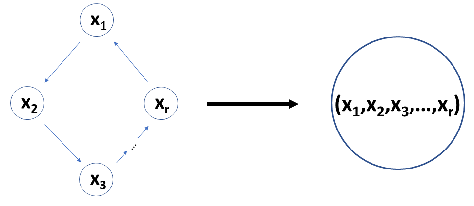
Figure 7: A cycle reduces to one node.

Reducing a cycle to one node does not affect our approach. This is because all nodes in the cycle necessarily occur always together in a subsystem containing any of the nodes from the cycle. Hence the subsystems obtained from a sparsity graph and the same sparsity graph where cycles have been reduced to single nodes coincide. Reducing all cycles leads to the condensation graph, where all strongly connected components ([7]) are reduced to one node. This can be performed in $\mathcal{O}(|V|+|E|)$, [7] Section 22.5, where $V$ denotes the set of nodes and $E$ the set of edges.

Similar arguments reveal that our approach does not allow a reduction if for example its corresponding graph is a path in which each branching is contained in a cycle; see Figure 8. And the same holds for sparsity graphs which are straight lines. Here the situation is even more drastic because the nodes are connected only by one incoming and one outgoing edge, and hence there is clearly much sparsity involved. Exploiting such sparse structures for the ROA is investigated by [36].

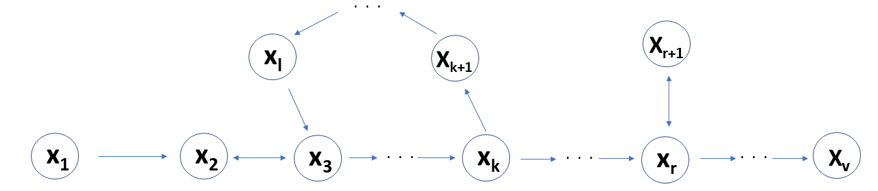
Figure 8: Straight paths with cycles.

The well known result stated in Lemma 1 contains the basic properties of leafs and their pasts that we need for the proof of the main theorem.

Lemma 1.

Any directed graph without cycles has at least one leaf. Furthermore, for directed graphs without cycles we have for the set $V$ of nodes that $V=\bigcup\limits_{x\text{ leaf}}\mathbf{P}(x)$.

Proof.

Let $W$ be a maximal path in the graph, i.e. a path that can’t be extended in $G$. Let $x$ be the last node in $W$. We claim that $x$ is a leaf. If $x$ is not a leaf then there exists an edge $(x,y)$ in $G$ for some node $y$. By maximality of $W$ we can’t add $y$ to $W$, that means the edge $(x,y)$ has been used before in $W$. This means that $W$ has visited $x$ before, i.e. there is a part of $W$ that connects $x$ to itself, i.e. a cycle – contradiction. For the remaining statement let $y$ be an arbitrary node. We can choose a longest path containing this node which has to end in a leaf $x$, hence $y$ is contained in the past of $x$. ∎

Before proving our main result we proceed as we did before in Proposition 2. As indicated in (19) we first establish a description of the ROA, MPI set, WA and GA by decomposing into subsystems according to the sparse structure of the dynamics for more general sparsity graphs than the cherry structure from Section 5.

Theorem 2.

Assume $X=X_{1}\times\cdots\times X_{r}$ and (for the ROA) $X_{\mathrm{T}}=X_{1,\mathrm{T}}\times\cdots\times X_{r,\mathrm{T}}$ for compact sets $X_{j},X_{j,T}\subset\mathbb{R}^{n_{j}}$ for $j=1,\ldots,r$. Assume the sparsity graph has no cycles. Let $x_{1},\ldots,x_{l}$ be the leafs of the sparsity graphs of $f$ with corresponding pasts $\mathbf{P}(x_{1}),\ldots,\mathbf{P}(x_{l})$. For the ROA let $T\in\mathbb{R}_{+}$. Then the ROA $R_{T}$, MPI set $M_{+}$, GA $\mathcal{A}$ and WA $\mathcal{A}_{w}$ are given by

$$R_{T}=\{x\in X:x_{\mathbf{P}(x_{i})}\in R_{T}^{i}\text{ for }i=1,\ldots,l\}$$ (20)

$$M_{+}=\{x\in X:x_{\mathbf{P}(x_{i})}\in M_{+}^{i}\text{ for }i=1,\ldots,l\}$$ (21)

$$\mathcal{A}=\{x\in X:x_{\mathbf{P}(x_{i})}\in\mathcal{A}^{i}\text{ for }i=1,\ldots,l\}$$ (22)

$$\mathcal{A}_{w}=\{x\in X:x_{\mathbf{P}(x_{i})}\in\mathcal{A}_{w}^{i}\text{ for }i=1,\ldots,l\}$$ (23)

where $R_{T}^{i},M_{+}^{i},\mathcal{A}^{i}$ and $\mathcal{A}^{i}_{w}$ denote the ROA, MPI set, GA and WA for the subsystem induced by the past of the leaf $x_{i}$ and $x_{\mathbf{P}(x_{i})}$ denotes the vector of states of $x$ that corresponds to the past of $x_{i}$.

Proof.

As in Proposition 1 the assumption on $X$ guarantees that the subsystems can be treated separately without concerning a violation of the state constraint due to states not contained in the subsystem. For the MPI set we can proceed in the same way as for the basic example (5) Proposition 2. That is why we omit the proof for the MPI set. The idea for the ROA, GA and WA are similar. We start with the ROA. Let $R$ denote the right hand side of (20). Let $x\in R$. We have to show that for the solution $x(\cdot)$ of the dynamical system with initial value $x$ we have $x(t)\in X$ for $t\in[0,T]$ and $x(T)\in X_{T}$. If we write $x(t)=(x_{1}(t),\ldots,x_{r}(t))$ this means we have to show $x_{k}(t)\in X_{k}$ for $t\in[0,T]$ and $x_{k}(T)\in X_{k,\mathrm{T}}$ for all $k=1,\ldots,r$. Fix $k\in\{1,\ldots,r\}$, by Lemma 1 and the assumption that the sparsity graph has no cycles it follows that $x_{k}\in\mathbf{P}(x_{i})$ for some leaf $x_{i}$. By definition of $R$ it follows $x_{k}(t)\in X_{k}$ for all $t\in[0,T]$ and $x_{k}(T)\in X_{k,\mathrm{T}}$ from $x\in R$. Hence $x\in R_{\mathrm{T}}$. For an element $x\in R_{\mathrm{T}}$ we have $x(t)=(x_{1}(t),\ldots,x_{r}(t))\in X_{1}\times\ldots X_{r}=X$ for all $t\in[0,T]$ and $x(T)=(x_{1}(T),\ldots,x_{r}(T))\in X_{1,\mathrm{T}}\times\ldots X_{r,\mathrm{T}}$. Let $x_{i}$ be a leaf. Then, clearly, $x_{\mathbf{P}(x_{i})}(t)\in\prod\limits_{x_{j}\in\mathbf{P}(x_{i})}X_{j}$ for $t\in[0,T]$ and $x_{\mathbf{P}(x_{i})}(T)\in\prod\limits_{x_{j}\in\mathbf{P}(x_{i})}X_{j,\mathrm{T}}$, which exactly means $x_{\mathbf{P}(x_{i})}\in R_{\mathrm{T}}^{i}$. For the GA we use the result for the MPI set and that $\mathcal{A}=M_{+}\cap M_{-}$ where $M_{+}$ denotes the MPI set and $M_{-}$ the maximum negatively invariant set, i.e. the MPI set in reversed time direction (see [33]). Hence the decoupling result is also true for the MNI set. We get

$$\mathcal{A} = M_{+}\cap M_{-}$$

$$= \{x\in X:x_{\mathbf{P}(x_{i})}\in M_{+}^{i}\text{ for }i=1,\ldots,l\}\cap$$

$$\{x\in X:x_{\mathbf{P}(x_{i})}\in M_{-}^{i}\text{ for }i=1,\ldots,l\}$$

$$= \bigcap\limits_{i=1}^{l}\{x\in X:x_{\mathbf{P}(x_{i})}\in M_{+}^{i}\cap M_{-}^{i}=\mathcal{A}^{i}\}$$

$$= \{x\in X:x_{\mathbf{P}(x_{i})}\in\mathcal{A}^{i}\text{ for }i=1,\ldots,l\}$$

where we used again $\mathcal{A}^{i}=M_{+}^{i}\cap M_{-}^{i}$ ([33] Definition 10.4. and Theorem 10.6.). Finally for the weak attractor we will show that the set from (23), denoted by $B_{w}$, is compact, pointwise attractive and contained in the weak attractor – hence by minimality of the weak attractor coincides with $\mathcal{A}_{w}$. Since $B_{w}$ is a closed subset of $X$ we get that $B_{w}$ is compact. To check that $B_{w}$ is attractive let $x\in M_{+}$ and $y$ be any accumulation point of the trajectory of $x$, i.e. there exists $\mathbb{R}_{+}\ni t_{m}\nearrow\infty$ with $\varphi_{t_{m}}(x)\rightarrow y$ as $m\rightarrow\infty$. Let $I_{i}$ denote $\mathbf{P}(x_{i})$ for $i=1,\ldots,k$. We get

$$\varphi^{I_{i}}(P_{I_{i}}x)=P_{I_{i}}\varphi_{t_{m}}(x)\rightarrow P_{I_{i}}y\text{ as }m\rightarrow\infty$$

from which follows that $P_{I_{i}}y$ is an accumulation point of the trajectory of the subsystem induced by ${I_{i}}$ starting at $P_{I_{i}}x$, and hence contained in the weak attractor for the subsystem induced by $I_{i}$. It follows $y\in B_{w}$, i.e. $B_{w}\supset\mathcal{A}_{w}$ and $B_{w}$ is attractive because the accumulation point $y$ was chosen arbitrarily. On the other hand from $\mathcal{A}_{w}$ being attractive it follows, due to (3), that $P_{I_{i}}(\mathcal{A}_{w})$ is attractive for the subsystem induced by $I_{i}$ for all $i=1,\ldots,k$. Hence $\mathcal{A}_{w}^{i}\subset P_{I_{i}}(\mathcal{A}_{w})$ because of minimality of $\mathcal{A}_{w}^{i}$. In particular we have $\mathcal{A}_{w}\subset B_{w}$. ∎

Remark 7.

As in the case of the MPI set shown in Proposition 2 in general the sets $R_{T}^{i}$, $\mathcal{A}^{i}$ and $\mathcal{A}_{w}^{i}$ do not coincide with $P_{\mathbf{P}(x_{i})}(R_{T})$, $P_{\mathbf{P}(x_{i})}(\mathcal{A})$ and $P_{\mathbf{P}(x_{i})}(\mathcal{A}_{w})$ respectively.

Remark 8.

Another typical approach to (global) attractors is via Lyapunov functions. A construction of Lyapunov functions based on the subsystems is possible as well and allows another approach to the decoupling result, which can be of independent interest.

This allows us to compute the desired sets based on computing them for the subsystems induced by the leafs.

Algorithm 1 (Decoupling procedure).

Input: A dynamical system induced by $f$ and a method for approximating/computing the ROA, MPI set or GA for an arbitrary dynamical system. Let $J_{1},\ldots,J_{N}$ be any partition of $\{1,\ldots,n\}$.

1. Reduce the cycles in the corresponding sparsity graph of $f$ as in Remark 6.

2. Compute approximations for subsystems: Let $x_{i_{1}},\ldots,x_{i_{l}}$ be the leafs of the corresponding sparsity graph after reducing the cycles. Use the given method to compute approximations $S_{i_{1}},\ldots,S_{i_{l}}$ of the ROAs, MPI sets or GAs respectively for the subsystems induced by the pasts of the leafs $x_{i_{1}},\ldots,x_{i_{l}}$.

3. Glue $S_{i_{1}},\ldots,S_{i_{l}}$ together as in Theorem 2 by

   $$S:=\{x\in X:x_{\mathbf{P}(x_{i_{r}})}\in S_{i_{r}}\text{ for }r=1,\ldots,l\}.$$

Next we show that the decoupling procedure preserves certain convergence properties. We consider the following two (pseudo) metrics on subsets on $\mathbb{R}^{n}$, one is the Hausdorff distance $\mathrm{dist}(\cdot,\cdot)$ and the other the Lebesgue measures discrepancy, defined by

$$d_{\lambda}(K_{1},K_{2}):=\lambda(K_{1}\Delta K_{2})$$ (24)

where $\lambda$ is the Lebesgue measure and $K_{1}\Delta K_{2}=(K_{1}\setminus K_{2})\cup(K_{2}\setminus K_{1})$ is the symmetric difference between the sets $K_{1}$ and $K_{2}$.

Theorem 3.

Let a dynamical system on $\mathbb{R}^{n}$ be induced by $f$ with state constraint $X=\prod\limits_{j=1}^{N}X_{j}$ for compact sets $X_{j}\subset\mathbb{R}^{n_{j}}$ and for the ROA let $X_{\mathrm{T}}=\prod\limits_{j=1}^{N}X_{j,\mathrm{T}}$ for a partition $J_{1},\ldots,J_{N}$ of $\{1,\ldots,n\}$ with $|J_{j}|=n_{j}$. Given a method for approximating the ROA, MPI set, WA or GA for an arbitrary dynamical systems, the following hold

1. in case of Hausdorff distance (induced by any norm on $\mathbb{R}^{n}$): If the method gives a convergent sequence of outer approximations $S_{k}$ of the desired set $S$, i.e. $S_{k}\supset S$ and

   $$\mathrm{dist}(S_{k},S)\rightarrow 0\;,\;\text{ as }k\rightarrow\infty.$$ (25)

   Then the decoupling procedure, Algorithm 1, produces a sequence of sets $S^{\prime}_{k}$ with

   $$\mathrm{dist}(S^{\prime}_{k},S)\rightarrow 0\;,\;\text{ as }k\rightarrow\infty.$$ (26)

   for $S$ denoting the desired set for the (sparse) dynamical system.

2. In case of Lebesgue measure: Let the sparsity graph of $f$ be acyclic and let $x_{i_{1}},\ldots,x_{i_{l}}$ be the leafs. Let $S^{\prime r}$ denote an approximation of the desired set $S^{r}$ for $r=1,\ldots,l$ for the subsystems induced by the leaf $x_{i_{r}}$. Then we have

   $$d_{\lambda}(S,S^{\prime}) = \leq\sum\limits_{r=1}^{l}\lambda(S^{r}\Delta S^{\prime r})\lambda(\prod\limits_{x_{k}\notin\mathbf{P}(x_{i_{r}})}X_{k})$$ (27)

   where $S$ is the desired set for the sparse dynamical system and $S^{\prime}$ the set obtained from Algorithm 1. In particular if a method produces approximations of $S^{i}$ that converge to $S^{i}$ with respect to $d_{\lambda}$ then the decoupling method produces a set that converges to $S$ with respect to $d_{\lambda}$.

Proof.

Let $x_{i_{1}},\ldots,x_{i_{l}}$ be the leafs in the sparsity graph obtained from the decoupling procedure and $S_{k}^{1},\ldots,S_{k}^{l}$ be the corresponding (converging outer) approximations of the desired sets for the subsystems induced by the leafs. For the first statement assume (26) does not hold. Then there exists a $\varepsilon>0$ and an unbounded subsequence $(k_{m})_{m\in\mathbb{N}}$ such that

$$\mathrm{dist}(S^{\prime}_{k_{m}},S)>\varepsilon$$ (28)

and we find points $x_{k_{m}}\in S^{\prime}_{k_{m}}$ with $\mathrm{dist}(x_{k_{m}},S)>\varepsilon$. By construction of $S^{\prime}_{k}$, boundedness of $S^{1},\ldots,S^{l}$ and the assumption (25) it follows that there exists $x\in\mathbb{R}^{n}$ and a subsequence of $(k_{m})_{m\in\mathbb{N}}$ which we will still denote by $(k_{m})_{m\in\mathbb{N}}$ such that $x_{k_{m}}\rightarrow x$ as $m\rightarrow\infty$. By assumption (25) there exist $y^{i}_{k_{m}}\in S^{i}$ for $i=1,\ldots,l$ with $\|y^{i}_{k_{m}}-(x_{k_{m}})_{\mathbf{P}(x_{i})}\|\rightarrow 0$ as $m\rightarrow\infty$. Hence also $y_{k_{m}}^{i}\rightarrow x_{\mathbf{P}(x_{i})}$ as $m\rightarrow\infty$ for $i=1,\ldots,l$. Because $S^{1},\ldots,S^{l}$ are closed it follows $x_{\mathbf{P}(x_{i})}\in S^{i}$ for $i=1,\ldots,l$ and by Theorem 2 we get $x\in S$. In particular we get

$$\varepsilon<\mathrm{dist}(x_{k_{m}},S)\leq\|x_{k_{m}}-x\|\rightarrow 0$$

as $m\rightarrow\infty$, which is a contradiction. For the second statement we get by the decoupling procedure Algorithm 1 that $S^{\prime}\subset X$ and $S\Delta S^{\prime}\subset\bigcup\limits_{r=1}^{l}\{x\in X:x_{\mathbf{P}(x_{i_{r}})}\in S^{r}\Delta S^{\prime r}\}$. Applying the Lebesgue measure to this inclusion gives

$$\lambda(S\Delta S^{\prime}) \leq \sum\limits_{r=1}^{l}\lambda\left(\{x\in X:x_{\mathbf{P}(x_{i_{r}})}\in S^{r}\Delta S^{\prime r}\}\right)$$

$$= \sum\limits_{r=1}^{l}\lambda(S^{r}\Delta S^{\prime r})\lambda(\prod\limits_{x_{k}\notin\mathbf{P}(x_{r})}X_{k}).$$

∎

In the next section we will state methods from [15], [17] and [34] that give converging (with respect to $d_{\lambda}$) approximations of the ROA, MPI set and GA. Then we have everything we need to state and prove our main theorem. Before doing so we first describe how to choose a good partition of nodes for the sparsity graph of a function $f$.

6.1 Selecting a partition

The choice of a partition of the states can influence the performance of the method strongly. Therefore, we start with factorizing the state space as finely as possible in order to decouple the dynamical system as much as possible.

Definition 7.

We say $X\subset\mathbb{R}^{n}$ factors with respect to a partition $J_{1},\ldots,J_{N}$ of $\{1,\ldots,n\}$ if there exist sets $X_{i}\subset\mathbb{R}^{n_{i}}$ where $n_{i}=|J_{i}|$ for $i=1,\ldots,n$ such that

$$X=\{x\in\mathbb{R}^{n}:P_{J_{i}}x\in X_{i}\text{ for }i=1,\ldots,N\}.$$

We say $J_{1},\ldots,J_{N}$ induces a factorization; the sets $X_{i}$ are given by $P_{j_{i}}X$.

Up to permutation of coordinates a factorization of $X$ states that $X$ is of the form $X=\prod\limits_{i=1}^{N}X_{i}$.

The following Lemma allows us to find the finest factorization of $X$ which will be useful in order to group only as many nodes in the sparsity graph together as needed.

Lemma 2.

There exists a minimal factorization for $X$; that is a factorization induced by $J_{1},\ldots,J_{N}$ of $X$, such that for any other factorization induced by $I_{1},\ldots,I_{M}$ we have for all $i=1,\ldots,M$ that $I_{i}=\bigcup\limits_{k:J_{k}\subset I_{i}}J_{k}$.

Proof.

We give a proof in the Appendix. ∎

A set $X$ that factors is of the norm $X=\prod\limits_{i=1}^{N}X_{i}$ up to a permutation of coordinates of $\mathbb{R}^{n}$. It is now clear that the partition obtained from Lemma 2 allows the finest decoupling of the dynamical system into subsystems, i.e. a decoupling into subsystems of smallest dimension.

7 Application to structured semidefinite programming outer approximations

As an illustrative example, we apply the decoupling procedure, Algorithm 1, to the convex optimization approaches region of attraction, maximum positively invariant set and global attractors from [15], [17] and [34].

For the ROA,MPI set and GA there exist representations in terms of solutions of infinite dimensional linear programs (see for example [36], [15], [18], [17] and [34]). Those provide converging outer approximations satisfying the conditions of Theorem 3 2. The decoupling procedure then allows to speed up the computations. Further we propose similar LPs that exploit the sparse structure even further but they have the disadvantage that they do not provide guaranteed convergence which is why we suggest to pair them with the convergent approach obtained from a hierarchy of SDPs from  [15], [17] and [34] with the decoupling procedure, thereby guaranteeing convergence by design.

At the beginning of this section we consider again general dynamical system on $\mathbb{R}^{n}$ with compact state constraint set $X\subset\mathbb{R}^{n}$ and no sparse structure. Sparse structures will be considered in subsections 7.3 and 7.4.

7.1 Linear program representations for the ROA, MPI set and GA

To state the LP from [15] for the ROA we need the Liouville operator $\mathcal{L}:\mathcal{C}^{1}([0,T]\times X)\rightarrow\mathcal{C}([0,T]\times X)$ that captures the dynamics, which is given by

$$\mathcal{L}v:=\frac{\partial}{\partial t}v+\nabla v\cdot f.$$ (29)

The dual LP from [15] is given by

(36)

In [17] an LP that relates to the MPI set was presented. This LP with discounting factor $\beta>0$ is given by

(42)

Based on the (dual) LP for the MPI set the following LP for the GA was proposed in [34] with discounting factors $\beta_{1},\beta_{2}>0$

$$d^{*}:=$$

s.t.

on X

on X

on X

on X

(43)

Remark 9.

The dual problem (36), (42) and (43) have the advantage that they give rise to outer approximations by the sets $w^{-1}([1,\infty)$, which get tight as feasible points $(v,w)$ or $(p,q,w)$ respectively get optimal. But this is typically not the case for primal feasible elements, which is why we don’t state the primal LPs here. Inner approximations can be approached in a similar way by using the LPs for inner approximations from [19] and [28]

7.2 Semidefinite programs for the ROA, MPI set, GA

In the previous subsection we have presented infinite dimensional LPs on the space of continuous functions – whose minimizers, or more precisely minimizing sequences, allow representations of the ROA, MPI set and GA. In this section we state a well known approach to such LPs that reduces the LP to a hierarchy of semidefinite programs (SDPs). Those SDP tightenings for the dual problems can be found in the corresponding papers (for example [15], [17], [34]). Combining the SDP approach with the decoupling procedure from Algorithm 1 we get a sparse approach towards approximating the ROA, MPI set and GA. We state the SDP procedure here to have a selfcontained sparse approach to convergent approximations for those sets.

For this approach it is necessary to assume additional algebraic structure of the problem because the dual LP tightens to a sum-of-squares problem, which leads to hierarchy of SDPs. This is a standard procedure and we refer to [22] or [21] for details.

Assumption 1.

The vector field $f$ is polynomial and $X\subset\mathbb{R}^{n}$ is a compact basic semi-algebraic set, that is, there exist polynomials $p_{1},\ldots,p_{i}\in\mathbb{R}[x]$ such that $X=\{x\in\mathbb{R}^{n}:p_{j}(x)\geq 0\text{ for }j=1,\ldots,i\}$. Further we assume that one of the $p_{j}$ is given by $p_{j}(x)=R^{2}-\|x\|_{2}^{2}$ for some large enough $R\in\mathbb{R}$. The set $X_{T}\subset\mathbb{R}^{n}$ satisfies similar conditions for polynomials $q_{j}$ for $j=1,\ldots,l$.

The idea for the SDP tightenings is first to reduce the space of continuous functions to the space of polynomials. The fact that the optimal value for the LP is not affected is justified by the Stone-Weierstraß theorem (and the existence of strictly feasible points). For the space of polynomials there is a natural way of reducing to a finite dimensional space, namely by bounding the total degree. That gives a sequence of finite dimensional optimization problems (in the coefficients of the polynomials). But those optimization problems are not tractable because testing non-negativity is a difficult task. The replacement of non-negativity as a sum-of-squares conditions allows a representation as an SDP. Finally convergence is guaranteed by Putinar’s positivstellensatz.

We give the SDP tightening for the ROA for a (non-sparse) dynamical system with constraint set $X$ with finite time horizon $[0,T]$ from [15]. The integer $k\in\mathbb{N}$ denotes the maximal total degree of the occurring polynomials and $d_{f}$ the total degree of the polynomial $f$.

(50)

for sum-of-squares polynomials $s_{1},a_{j},b^{1}_{l},b\in\mathbb{R}[t,x]$, $s_{2},s_{3},s_{4},c_{j},e_{j}\in\mathbb{R}[x]$ for $j=1,\ldots,i$; such that all occurring polynomials in the SDP (50) have degree at most $k$. The vector $\bm{\lambda}$ denotes the vector of moments of the Lebesgue measure on $X$ and $\mathbf{w}$ denotes the coefficients of the polynomial $w$, such that $\langle\mathbf{w},\bm{\lambda}\rangle=\int\limits_{X}w(x)\;d\lambda$.

The SDPs for the MPI set and GA are similar – the non-negativity constraint is replaced by a SOS certificate. We omit stating the SDPs here explicitly (they can be found in [17] and [34]).

By [15], [17] and [34] the sequences $d_{k}^{*}$ of optimal values of the corresponding SDPs from (50) for the ROA, for the MPI set and for the GA converge monotonically from above to the Lebesgue measure of the corresponding sets. Further the corresponding semi-algebraic set

$$S_{k}:=w^{-1}([1,\infty)]=\{x\in X:w(x)\geq 1\}$$ (51)

are outer approximations that get tight (with respect to Lebesgue measure discrepancy) when $(v,w)$ – similarly for the MPI set and GA.

7.3 Decoupling SDPs using sparsity: the algorithm

Now we have everything we need to state our main algorithm and prove our main theorem. The main ingredients are Theorem 3 and convergence properties for the hierarchy of SDPs.

Algorithm 2.

Let $J_{1},\ldots,J_{N}$ be a partition of $\{1,\ldots,n\}$ with $|J_{j}|=n_{j}$ and a dynamical system on $\mathbb{R}^{n}$ be induced by a polynomial $f$ with state constraint $X=\prod\limits_{j=1}^{N}X_{j}$, for compact basic semialgebraic sets $X_{j}\subset\mathbb{R}^{n_{j}}$ satisfying Assumption 1 (and for the ROA $X_{T}=\prod\limits_{j=1}^{N}X_{j,T}$ for compact basic semialgebraic $X_{T,j}\subset\mathbb{R}^{n_{j}}$) for $j=1,\ldots,N$. Fix the maximum degree $k\in\mathbb{N}$ of polynomials occurring in the SDPs.

1. Reduce the cycles in the corresponding dimension weighted sparsity graph of $f$ as in Remark 6.

2. Compute outer approximations of the ROA, MPI set or GA for subsystems by the SDPs (50), respectively from [17], [34]: Let $x_{i_{1}},\ldots,x_{i_{l}}$ be the leafs of the corresponding sparsity graph after reducing the cycles. Use the SDPs (50) respectively their variants for the MPI set or global attractors for polynomials up to degree $k$ to compute approximations $S^{(k)}_{1},\ldots,S^{(k)}_{l}$ of the ROAs, MPI sets or GA respectively for the subsystems induced by the pasts of the leafs $x_{i_{1}},\ldots,x_{i_{l}}$.

3. Glue $S^{(k)}_{1},\ldots,S^{(k)}_{l}$ together as in Theorem 2 by

   $$S^{(k)} := \{x\in X:x_{\mathbf{P}(x_{i_{r}})}\in S^{(k)}_{r}\text{ for }r=1,\ldots,l\}$$

   $$= \{x\in X:w_{k}^{i}(x_{\mathbf{P}(x_{i})})\geq 1\text{ for }i=1,\ldots,l\}.$$

The second equality in (iii.) follows immediately from (51).

Before stating the main theorem we remind of the definition (4) of the largest dimension weighted past $\omega$ which is the number of variables appearing in the largest subsystem.

Theorem 4.

Algorithm 2 produces converging outer approximations of the ROA, MPI set or GA respectively, i.e. $S^{(k)}\supset S$ for all $k\in\mathbb{N}$ and

$$d_{\lambda}(S^{(k)},S)=\lambda(S^{(k)}\Delta S)\rightarrow 0\text{ as }k\rightarrow\infty$$

where $S$ denotes the ROA, MPI set or GA respectively for the dynamical system. The complexity of the corresponding SDPs that need to be solved in Algorithm 2 is determined by $\omega$.

Proof.

This follows immediately from the convergence results of [15], [17], [34] and Theorem 3 because the largest SDP, i.e. the SDP involving the most variables, that occurs is induced by the subsystem whose leaf has the largest weighted past and this SDP acts on sum-of-squares multipliers on $\omega$ variables. ∎

That the complexity of the SDPs is determined by $\omega$ is the reason why this approach is useful to reduce complexity. The SDPs obtained by SOS hierarchies grow combinatorically in the number of variables and the degree bound $k$. The number of variables used in each branch of the tree reduces the number of variables for the remaining problems. To make this more precise let us have a look at the basic branching as in Figure (5). Let $n_{1},n_{2},n_{3}$ be the number of variables in $x_{1},x_{2},x_{3}$; note that for (50) an additional dimension appears due to the time parameter. Let $k$ be the degree used for the SDP (50). Then the size of the largest sum-of-squares multiplier for the full system is

$$\binom{n_{1}+n_{2}+n_{3}+1+\frac{k}{2}}{\frac{k}{2}}$$

while for the subsystems it is

$$\binom{n_{1}+n_{2}+1+\frac{k}{2}}{\frac{k}{2}}\text{ and }\binom{n_{1}+n_{3}+1+\frac{k}{2}}{\frac{k}{2}}.$$

For general graphs it follows similarly that the more the graph separates into subsystems the more effective this approach gets.

Hence we see that the reduction in the number of variables is significant if the dynamics is strongly separated, i.e. pasts of the leafs overlap less, i.e. $n_{i}$ and $\phi_{i}$ are small compared to $n$ and $\Phi$. This is what we would expect because strong separation tells us that fewer interactions are needed in order to describe the system.

Remark 10.

Treating the subsystems separately by the decoupling procedure has another advantage. Namely it allows to take properties of the subsystems into account. Particularly for the SDP approach this allows for example the use of different degrees for the hierarchies of different subsystems. This can be useful if the hierarchy for some subsystems allow the use of low degrees to already capture the dynamics well while for other subsystems high degrees are required to obtain accurate approximations. For the whole system this typically means that also a high degree for the SDP hierarchy is needed (in order to capture the dynamics of the more complex subsystem).

7.4 Sparse improvement

We propose a slightly adapted LP that allows a further (sparse) improvement on the outer approximation while maintaining the reduced computational complexity.

For the rest of this section assume that the sparsity graph of $f$ with respect to a given partition is acyclic and has leafs $x_{i_{1}},\ldots,x_{i_{l}}$. Let $I_{1},\ldots,I_{l}$ be the set of indices corresponding to the nodes in the past of $x_{i_{1}},\ldots,x_{i_{l}}$ and let $X_{I_{r}}:=\prod\limits_{j\in I_{r}}X_{j}$ denote the constraint space for the subsystem induced by the past of $x_{i_{r}}$ for $r=1,\ldots,l$. The set $x_{I_{r}}$ denotes the projection of $x\in X$ onto $X_{I_{r}}$, i.e. the components of $x$ corresponding to $I_{r}$. Similarly for the function $f$ let $f_{I_{r}}$ denote the components of $f$ corresponding to the index set $I_{r}$. Let $n_{r}$ be the dimension of the state space for the subsystem induced by the past of $x_{i_{r}}$, i.e. $X_{I_{r}}\subset\mathbb{R}^{n_{r}}$.

It is possible to combine the LPs for the subsystems but such that the constraints only act on functions on $X_{I_{r}}$ for $r=1,\ldots,l$. We propose the following dual sparse LP for the ROA

(59)

Where $\mathcal{L}_{r}$ denotes the Liouville operator (29) on the subsystem induced by the past of $x_{i_{r}}$.

The LP is sparse because the functions $w^{r},v^{r}$ only depend on $x_{I_{r}}$ instead of $x$. For the corresponding SDP we choose the SOS multiplier to only depend on the variables $x_{I_{r}}$.

Remark 11.

We have summed the corresponding inequalities of the LP (36) for the subsystems. This has the advantage that the set of feasible points for the LP (and the corresponding SDP) is larger. On the other hand it enforces less structure on the feasible points. This can potentially hamper convergence of the approximations. This undesirable property can be avoided by intersecting with the approximations coming from the fully decoupled approach; this is formally stated in Theorem 5.

Similar to the set constructed by the decoupling based on the SDP hierarchy in (51) we can construct a superset of the ROA based on feasible sets for the sparse LP (59).

Proposition 3.

Let $(w^{1},v^{1},w^{2},v^{2},\ldots,w^{l},v^{l})$ be feasible. Then

$$\{x\in X:\sum\limits_{r=1}^{l}w^{r}(x_{I_{r}})\geq l\}\supset R_{T}.$$ (60)

Proof.

We can apply Lemma 2 from [15] to the functions $v(x):=\sum\limits_{r=1}^{l}v^{r}(x_{I_{r}})$ and $w(x):=\sum\limits_{r=1}^{l}w^{r}(x_{I_{r}})$ and the conclusion follows. ∎

Similar arguments for the LPs (42) and (43) for the MPI set and the GA lead to sparse LPs for the MPI set and GA and Proposition 3 holds in an analogue way.

We can enforce the sparse structure of the LPs (59)to the corresponding hierarchy of SDPs; by that we mean that instead of replacing the non-negativity constraint by an SOS constraint with polynomials on $X$ we only use SOS polynomials on the spaces $X_{I_{r}}$. This reduces the complexity due to the possibility to work with the smaller spaces $\mathbb{R}[x_{I_{1}}],\ldots,\mathbb{R}[x_{I_{l}}]\subset\mathbb{R}[x]$ similar to treating the subsystems separately as in the previous subsection.

Even though this approach has similar computational complexity – because the largest SOS multiplier acts on $\omega$ variables – we can’t guarantee convergence. This is why we need to pair this method with the convergent method based on the decoupling the dynamical systems to obtain a convergent sequence of outer approximation.

Theorem 5.

Under the assumption of Theorem 4 let $S^{(k)}$ for $k\in\mathbb{N}$ be the outer approximation of the ROA from (iii.) and $Y^{(k)}$ be the sets obtained from (60) by optimal points $(w^{r},v^{r})_{r=1,\ldots,l}$ of the corresponding sparse SDPs for (59). Then $S^{(k)}\cap Y^{(k)}$ is a converging (with respect to $d_{\lambda}$) outer approximation of the ROA. The largest occurring SOS multiplier acts on $\omega$ variables.

Proof.

By Propositions 3 we have $S^{(k)}\supset S^{(k)}\cap Y^{(k)}\supset S$ where $S$ denotes the desired set. Hence convergence follows from convergence of $S^{(k)}$ stated in Theorem 4. By the enforced sparse structure of the SDPs for the sparse LP (59) the largest SOS multiplier occurs corresponding to the subsystem induced by a leaf with the state space of largest dimension; hence it acts on $\omega$ variables. ∎

Remark 12.

Arguments, analogue to the ones in this section, lead to sparse improvements for the MPI set and global attractor and Theorem 5 holds in a similar way.

8 Numerical examples

8.1 Cherry structure

Cherry structures are the most sparse structures for our framwork. They occur for instance in Dubins car and the 6D Acrobatic Quadrotor [5]. We illustrate a larger (more artificial) example of a cherry structure. We consider the interconnection of Van der Pol oscillators as in Figure 9.

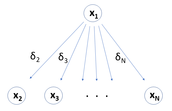
Figure 9: Interconnection of Van-Der Pol oscillators in a cherry structure.

For the leaf nodes $x^{2},\ldots,x^{N}$, the dynamics is

$$\dot{x}^{i}_{1} =2x^{i}_{2}$$

$$\dot{x}^{i}_{2} =-0.8x^{i}_{1}-10[(x^{i}_{1})^{2}-0.21]x^{i}_{2}+\delta_{i}x_{1}^{1}.$$

For the root note $x^{1}$, the dynamics is

$$\dot{x}^{1}_{1} =2x^{1}_{2}$$

$$\dot{x}^{1}_{2} =-0.8x^{1}_{1}-10[(x^{1}_{1})^{2}-0.21]x^{1}_{2}.$$

We illustrate the decoupling procedure by computing outer approximations of the MPI set of this system with respect to the constraint set $[-1.2,1.2]^{2N}$. We carry out the computation for degree $k=8$ and $N=10$, resulting in a total dimension of the state-space equal to 20. The optimal decoupling in this case is into subsystems $(x^{1},x^{i})$, $i=2,\ldots,N$, each of dimension four. Figure 10 shows the sections of the MPI set outer approximations when the value at the root node is fixed at $[0.5,-0.1]$. The computation time was 12 seconds. Next we carried out the the computation with $k=8$ and $N=26$, resulting in state-space dimension of 52. Figure 11 shows the sections of the MPI set outer approximations when the value at the root node is fixed at $[0.5,-0.1]$. The total computation time was 40.3 seconds. It should be mentioned that these problems in dimension 20 or 52 are currently intractable without structure exploitation. Here the sparse structure allowed for decoupling in $9$ respectively $25$ problems in 4 variables, which were solved in less than a minute in total.

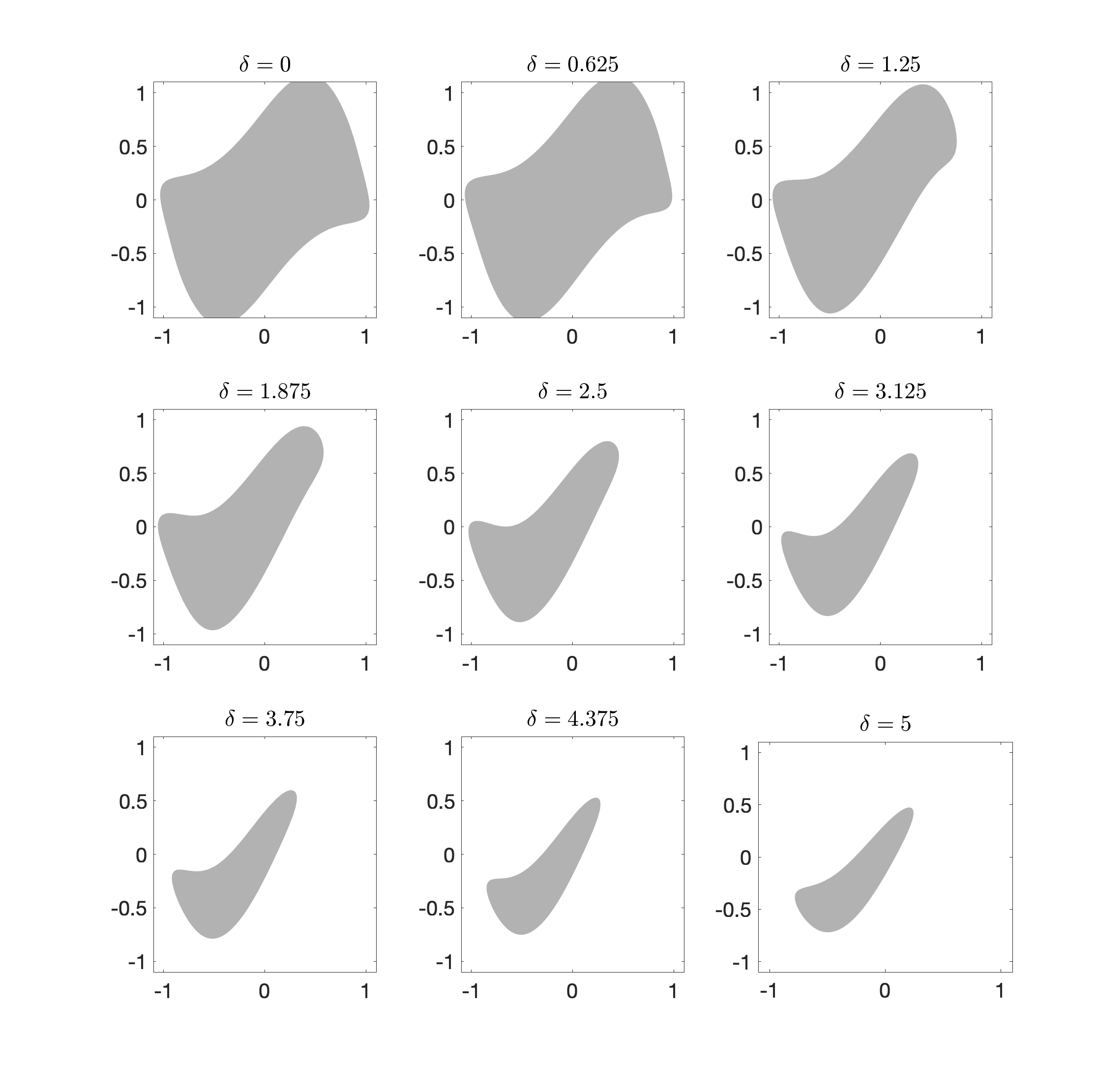
Figure 10: Van der Pol oscillators in a cherry structure: The figure shows the outer approximations of the MPI set for $k=8$ and $N=10$ for the subsystems given by the cherry–branches.

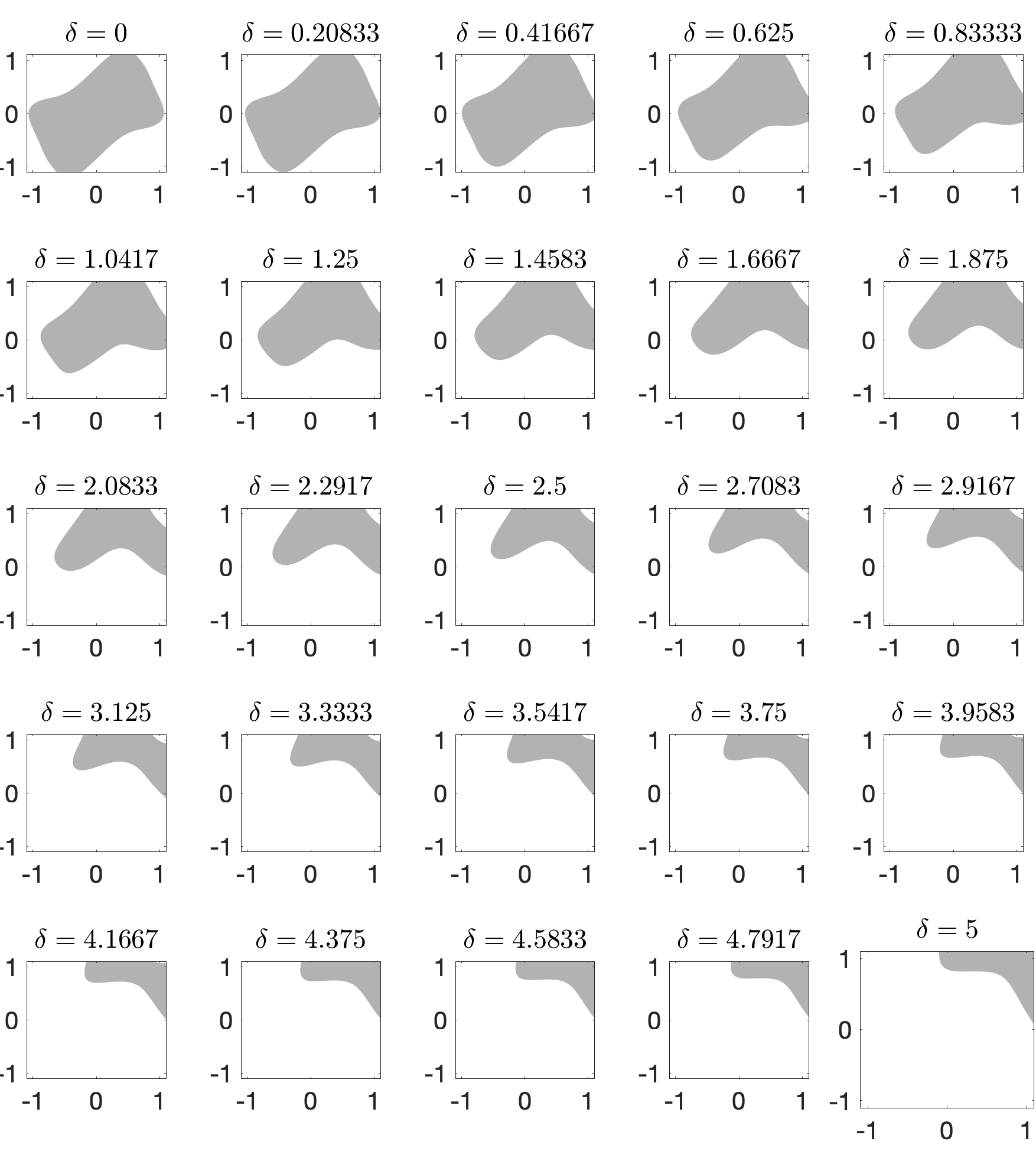
Figure 11: Van der Pol oscillators in a cherry structure: The figure shows the outer approximations of the MPI set for $k=8$ and $N=26$ for the subsystems given by the cherry–branches

8.2 Tree structure

We thank Edgar Fuentes for pointing out to us that radial distribution networks provide common examples of tree structures [4]. In a similar fashion we consider a network of Van der Pol oscillators as in Figure 12.

The coupling is as in the previous example from the first component of the predecessor state to the second component of the successor state. The coupling intensity $\delta$ is set to 0.1 for each edge. The goal is to compute the MPI set with respect to the constraint set $[-1.2,1.2]^{10}$. The optimal decoupling is now into 3 subsystems given by $(x^{1},x^{2},x^{4})$, $(x^{1},x^{2},x^{5})$, $(x^{1},x^{3})$; the respective dimensions are $6$, $6$ and $4$. Figure 13 shows six random sections of the ten dimensional MPI set outer approximation computed by our approach with degree $k=8$. Even though the the overall state-space dimension 10 is less than it was in our previous example, the computation time of 285 seconds is higher since the maximum dimension of the subsystems is higher.

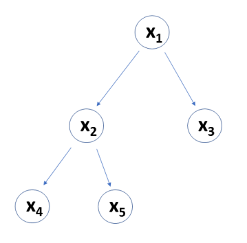
Figure 12: Interconnection of Van-Der Pol oscillators in a tree structure.

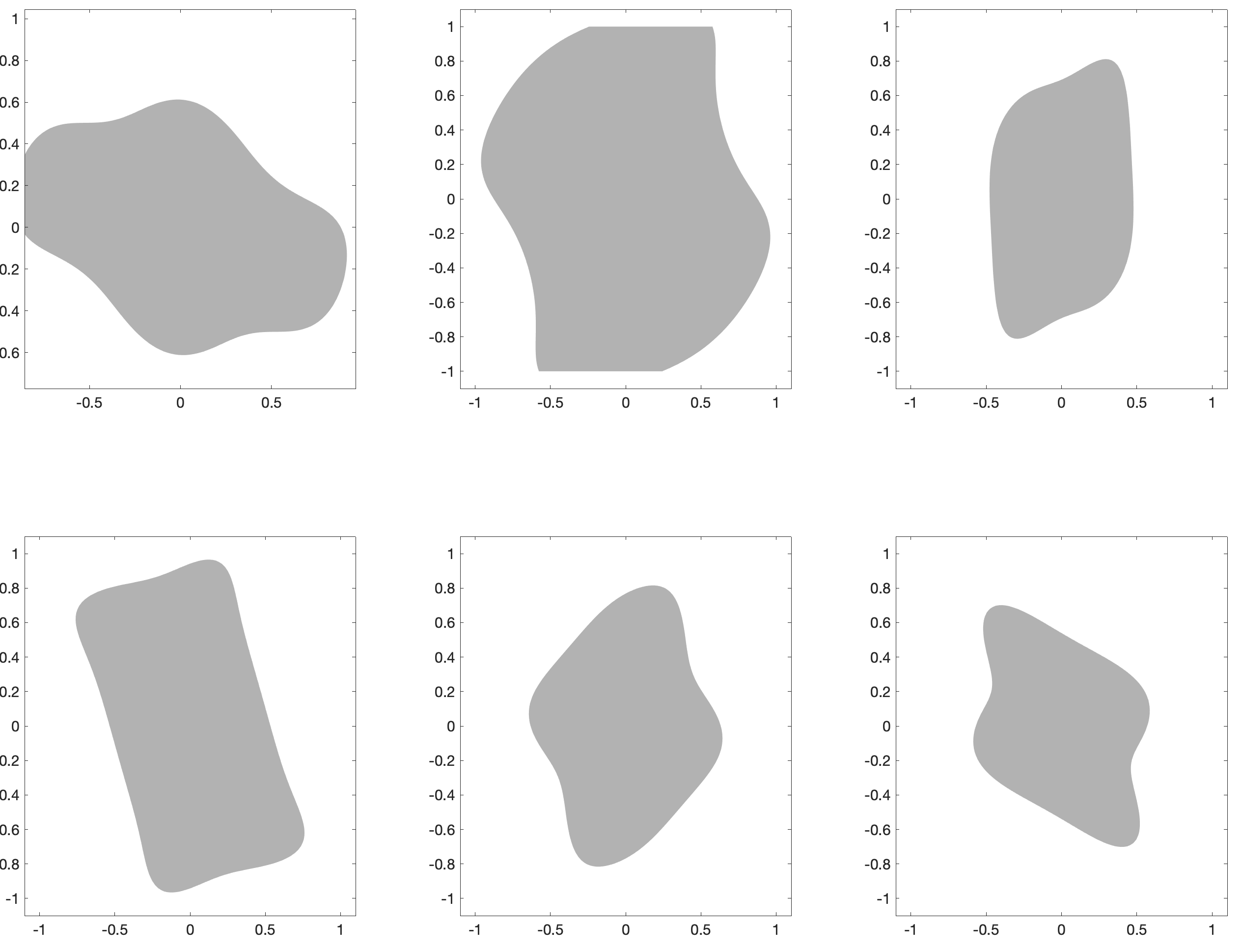
Figure 13: Van der Pol oscillators in a tree structure: Random projections of the outer approximation to the ten dimensional MPI set.

9 Conclusion

We presented a decomposition of several important sets related to nonlinear dynamical systems based on their correspondences for subsystems of the dynamical system. This was motivated by [5] and extended from the region of attraction to also the maximum positively invariant set as well as GA and WA. Compared to [5] we focused on the uncontrolled but state–constrained case and showed how this concept can be generalized for general dynamical systems on $\mathbb{R}^{n}$. We showed that this decomposition gives rise to methods for computing these sets from their correspondences for the subsystems. Using the works [15], [17] and [34] we presented a method that provides a converging sequence of outer approximations based on convex optimization problems, while exploiting the underlying structure.

We believe that decomposing the dynamical system into subsystems as presented here can be beneficial for other objectives such as constructions of Lyapunov functions or invariant measures to name just two. It may also be of interest to exploit sparsity for extreme value computation, building on [12]. Another direction of future work is the inclusion of control, i.e., the computation of the region of attraction with control, the maximum controlled invariant set and optimal control. Utilizing this approach in a data-driven setting, building on [16], is another possible generalization.

Sparsity in the dependence of the dynamics of the states is not the only structure of $f$ that can be exploited. If for example $f$ is a polynomial, then the algebraic structure of $f$ can be investigated as in [41] for instance. In addition, more general sparse structures should be investigated as we have seen that our approach treats straight paths or cycles as subsystems – in the same way as if all the corresponding nodes were fully connected. Work in this direction was done in [36].

Additional reduction techniques, as for example symmetry, can be combined with our approach. Decoupling into subsystems maintains symmetry structures (for the subsystems), so merging our approach with for example the symmetry argument in [9] can be done by first decoupling into subsystems and then exploiting symmetries of the subsystems (independently).

The aim of investigating subsystems is to understand intrinsic lower dimensional dynamics of the dynamical system. But this is also where a fundamental limitation arises from our notion of subsystems because it is not coordinate-free. This can be seen for example by a linear dynamical system $\dot{x}=Ax$ for diagonalizable matrix $A\in\mathbb{R}^{n\times n}$ with non-zero entries. Since every entry of $A$ is non-zero the sparsity graph is the complete graph while after a change of coordinates that diagonalizes $A$ (and transforms the constraint set to a set that factors) the corresponding sparsity graph for this dynamical system consists of isolated nodes, i.e. there are no edges at all. While a coordinate free formulation would describe dynamical systems intrinsically embedded in the whole system, the coordinate dependent formulation is only able to track such embedded dynamics that arise from projections along canonical coordinates. This restrictive notion of subsystems comes with the advantage of an easy practical access by explicitly finding subsystems whenever there are any; and hence should be viewed as a practical attempt to the task of finding intrinsic subsystems. We aim to investigate a coordinate free formulation of the main results in future work.

10 Appendix: proof of Lemma 2

Proof.

We look at the set $T:=\{J\subset\{1,\ldots,n\}:J\text{ and }\{1,\ldots,n\}\setminus J\text{ induces a factorization of }X\}$. The set $T$ is the collection of all partitions consisting of only two sets, such that they induce a factorization of $X$. We will see that $T$ contains minimal elements (with respect to inclusion); these will give rise to the desired factorization of $X$. We start with the following properties of $T$.

1. $T$ is non-empty.
   $J=\{1,\ldots,n\}$ is contained in $X$ because it induces the trivial factorization $X$ of factoring into itself.

2. $T$ is closed with respect to taking the complement in $\{1,\ldots,n\}$.
   Let $J\in T$ then $J^{c}:=\{1,\ldots,n\}\setminus J\in T$ because $J^{c},J$ is a partition that induces the same factorization as $J,J^{c}$.

3. $T$ is closed with respect to intersections.
   Let $J_{1},J_{2}\in T$ with corresponding sets $X_{1}:=P_{J_{1}}(X)$, $X_{2}:=P_{J_{1}^{c}}(X)$ and $Y_{1}:=P_{J_{2}}(X),Y_{2}:=P_{J_{2}^{c}}(X)$. Let $J:=J_{1}\cap J_{2}$ and $I:=\{1,\ldots,n\}\setminus J$. We claim $J,I$ induces a factorization. Therefore let $Z_{1}:=P_{J}(X)$ and $Z_{2}:=P_{I}(X)$. We need to show that we have

   $$X=X^{\prime}:=\{x\in\mathbb{R}^{n}:P_{J}(x)\in Z_{1},P_{I}(x)\in Z_{2}\}.$$ (61)

   For any $x\in X$ we have $x\in X^{\prime}$ by definition of $Z_{1}$ and $Z_{2}$. Let $x^{\prime}\in X^{\prime}$. By definition of $Z_{1}$ there exists $x_{1}\in X$ with $P_{J}(x_{1})=P_{J}(x^{\prime})$. From $J_{1}\in T$ it follows $P_{J_{1}}(x_{1})\in X_{1}$. Since $I\supset J_{1}^{c}$ it follows $P_{J_{1}^{c}}(x_{1})\in P_{J_{1}^{c}}(P_{I}(X))=P_{J_{1}^{c}}(X)=X_{2}$. Since $J_{1},J_{1}^{c}$ induces a factorization we get that the element $x_{2}\in\mathbb{R}^{n}$ with $P_{J_{1}}(x_{2})=P_{J_{1}}(x_{1})$ and $P_{J_{1}^{c}}(x_{2})=P_{J_{1}^{c}}(P_{I}(x^{\prime}))$ belongs to $X$. If we repeat this process with $J_{1}$ replaced by $J_{2}$ we find an element $x_{3}\in X$ such that $P_{J}(x_{3})=P_{J_{1}\cap J_{2}}(x_{3})=P_{J_{1}\cap J_{2}}(x^{\prime})$ and $P_{I}(x_{3})=P_{J_{1}^{c}\cup J_{2}^{c}}(x_{3})=P_{J_{1}^{c}\cup J_{2}^{c}}(x^{\prime})$, i.e. $x^{\prime}=x_{3}\in X$.

4. $T$ is closed with respect to taking union.
   Let $J_{1},J_{2}\in T$. Then $J_{1}\cup J_{2}=(J_{1}^{c}\cap J_{2}^{c})^{c}\in T$.

It follows that $T$ is a (finite) topology and hence there exists a minimal basis of $T$ (consisting of the smallest neighbourhoods of each point), i.e. for each $i\in\{1,\ldots,n\}$ define $U_{i}:=\bigcap\limits_{J\in T:i\in J}J\in T$. Those $U_{i}$ are minimal elements in $T$ containing $i$, and hence their unions covers $\{1,\ldots,n\}$. Further for $i\neq k$ the sets $U_{i}$ and $U_{k}$ are either identical or disjoint, otherwise intersecting them would create smaller non-empty elements in $T$. Let $J_{1},\ldots,J_{N}$ be the partition induced by the sets $U_{i}$, i.e. for all $k=1,\ldots,N$ the set $J_{k}$ is given by some $U_{i}$ and $J_{1},\ldots,J_{N}$ is a partition. We claim that this defines the finest partition that factorizes $X$. First let $I_{1},\ldots,I_{M}$ induce a factorization of $X$. Let $1\leq k\leq M$. Then $I_{k},I_{k}^{c}$ induces a partition because $I_{1},\ldots,I_{M}$ already induces a partition. That means $I_{k}\in T$ and since the $U_{i}$ build a basis we have $I_{k}=\bigcup\limits_{i\in J_{k}}U_{i}$. It remains to show that $J_{1},\ldots,J_{N}$ defines a partition. For each $1\leq k\leq N$ there exist sets $X_{k}$ (and $X_{k}^{\prime}$) such that

$$X=\{x\in\mathbb{R}^{n}:P_{J_{k}}(x)\in X_{k},P_{J_{k}^{c}}(x)\in X_{k}^{\prime}\}.$$ (62)

We claim $X=\{x\in\mathbb{R}^{n}:P_{J_{i}}(x)\in X_{i}\text{ for }i=1,\ldots,N\}$. It suffices to show that $\{x\in\mathbb{R}^{n}:P_{J_{i}}(x)\in X_{i}\text{ for }i=1,\ldots,N\}\subset X$. Therefore let $x\in\mathbb{R}^{n}$ such that $P_{J_{i}}(x)\in X_{i}$. Because $J_{2}\in T$ it follows from $P_{J_{2}}(x)\in X_{2}$ that there exists a $x^{2}\in X$ with $P_{J_{2}}(x^{2})=P_{J_{2}}(x)$. Hence it follows $P_{J_{1}^{c}}(x^{2})\in X^{\prime}_{1}$. In particular the element

$$\tilde{x}^{2}=(\tilde{x}^{2}_{i})_{i=1,\ldots,n}\text{ with }\tilde{x}^{2}_{i}=\begin{cases}x_{i},&i\in J_{1}\\ x^{2}_{i},&i\in J_{1}^{c}\end{cases}$$ (63)

belongs to $X$ and satisfies $\tilde{x}^{2}_{i}=x_{i}$ for $i\in J_{1}\cup J_{2}$. Now we can continue this process for the new partition $(J_{1}\cup J_{2}),J_{3},\ldots,J_{N}$ and find an element $\tilde{x}^{3}\in X$ with $\tilde{x}^{3}_{i}=x_{i}$ for $i\in J_{1}\cup J_{2}\cup J_{3}$. Continuing until we have reached $J_{N}$ we find that finally $x=\tilde{x}^{N}\in X$. ∎

References

- [1] d’Andréa-Novel, Brigitte, Jean-Michel Coron, and Wilfrid Perruquetti, Small-Time Stabilization of Homogeneous Cascaded Systems with Application to the Unicycle and the Slider Examples, SIAM Journal on Control and Optimization 58.5 (2020): 2997-3018.
- [2] F. Blanchini, Set invariance in control, Automatica, 35(11), pp. 1747–1767, 1999.
- [3] F. Bullo, Lectures on network systems. Vol. 1., Santa Barbara, CA: Kindle Direct Publishing, 2019.
- [4] M. Chakravorty, D. Das, Voltage stability analysis of radial distribution networks, International Journal of Electrical Power & Energy Systems, 23, Issue 2, 2001,pp. 129–135.
- [5] M. Chen, S. L. Herbert,M. S. Vashishtha, S. Bansal and C. J. Tomlin, Decomposition of Reachable Sets and Tubes for a Class of Nonlinear Systems, IEEE Transactions on Automatic Control, vol. 63, no. 11, 2001, pp. 3675–3688.
- [6] G. Chesi, Domain of attraction; analysis and control via SOS programming, Lecture Notes in Control and Information Sciences, Vol. 415, Springer-Verlag, Berlin, 2011.
- [7] T. H. Cormen, C.E. Leiserson, R. L. Rivest and C. Stein, Introduction to Algorithms, Second Edition, MIT Press and McGraw-Hill, 2001.
- [8] M. Dellnitz and O. Junge, Set oriented numerical methods for dynamical systems, in Handbook of Dynamical Systems, Vol. 2, 2002, North-Holland, Amsterdam, pp. 221–264.
- [9] G. Fantuzzi and D. Goluskin, Bounding Extreme Events in Nonlinear Dynamics Using Convex Optimization, SIAM J. Appl. Dyn. Syst., 19(3), 2020, pp. 1823–-1864.
- [10] P. Giesl and S. Hafstein, Review on computational methods for Lyapunov functions, Discrete & Continuous Dynamical Systems - B, 20 (8), 2015, pp. 2291–2331.
- [11] Puskorius, Gintaras V., and Lee A. Feldkamp, Neurocontrol of nonlinear dynamical systems with Kalman filter trained recurrent networks, IEEE Transactions on neural networks 5.2 (1994): 279-297.
- [12] D. Goluskin, Bounding extrema over global attractors using polynomial optimisation, Nonlinearity, 33, 2020, 4878.
- [13] Granger, Clive WJ, Investigating causal relations by econometric models and cross-spectral methods, Econometrica: journal of the Econometric Society, pp. 424–438, 1969.
- [14] D. Henrion, M. Korda and J. B. Lasserre, Moment-sos Hierarchy, The: Lectures In Probability, Statistics, Computational Geometry, Control And Nonlinear PDEs,” World Scientific, Vol. 4, 2020.
- [15] D. Henrion and M. Korda, Convex Computation of the Region of Attraction of Polynomial Control Systems, IEEE Transactions on Automatic Control, vol. 59, no. 2, 2014, pp. 297–312.
- [16] M. Korda, Computing controlled invariant sets from data using convex optimization, SIAM Journal on Control and Optimization, vol. 58, no. 5, 2020, pp. 2871–2899.
- [17] M. Korda, D. Henrion and C. N. Jones, Convex computation of the maximum controlled invariant set for polynomial control systems, SIAM Journal on Control and Optimization, 52(5), 2014, pp. 2944-2969.
- [18] M. Korda, D. Henrion and C. N. Jones, Controller design and region of attraction estimation for nonlinear dynamical systems, IFAC Proceedings Volumes, Volume 47, Issue 3, 2014, pp. 2310–2316.
- [19] M. Korda, D. Henrion and C. N. Jones, Inner approximations of the region of attraction for polynomial dynamical systems, IFAC Proceedings Volumes, Volume 46, Issue 23, 2013, pp. 534–539.
- [20] A. T. Kwee, M. F. Chiang, P. K. Prasetyo and E. P. Lim, Traffic-cascade: Mining and visualizing lifecycles of traffic congestion events using public bus trajectories. In Proceedings of the 27th ACM International Conference on Information and Knowledge Management, pp. 1955–1958, 2018.
- [21] J. B. Lasserre, Global optimization with polynomials and the problem of moments, SIAM Journal on optimization, 11(3), 2001, pp. 796–817, 2001.
- [22] J. B. Lasserre, Moments, positive polynomials and their applications, Imperial College Press, London, UK, 2009.
- [23] M. Li, X. Zhou, Y. Wang, L. Jia and M. An, Modelling cascade dynamics of passenger flow congestion in urban rail transit network induced by train delay, Alexandria Engineering Journal,61, 11, pp. 8797–8807, 2022.
- [24] Dedi Liu, Shenglian Guo, Pan Liu, Lihua Xiong, Hui Zou, Jing Tian, Yujie Zeng, Youjiang Shen, Jiayu Zhang, Optimisation of water-energy nexus based on its diagram in cascade reservoir system, Journal of Hydrology, Volume 569, 2019, Pages 347-358.
- [25] Lopez, J. C., Vergara, P. P., Lyra, C., Rider, M. J. and Da Silva, L. C., Optimal operation of radial distribution systems using extended dynamic programming. IEEE Transactions on Power Systems, 2017, 33(2), 1352-1363.
- [26] J. Löfberg, YALMIP : A toolbox for modeling and optimization in MATLAB. In Proc. IEEE CCA/ISIC/CACSD Conference, Taipei, Taiwan, 2004.
- [27] Mohr, Ryan, and Mezić, Igor, Koopman Spectrum and Stability of Cascaded Dynamical Systems, The Koopman Operator in Systems and Control, Springer, Cham, 2020. 99-129.
- [28] A. Oustry, M. Tacchi and D. Henrion, Inner approximations of the maximal positively invariant set for polynomial dynamical systems, arXiv preprint arXiv:1903.04798, 2019.
- [29] Paluš, Milan and Krakovská, Anna and Jakubík, Jozef and Chvosteková, Martina, Causality, dynamical systems and the arrow of time, Chaos: An Interdisciplinary Journal of Nonlinear Science, 28, 7, 075307, 2018.
- [30] J. Peters, S. Bauer and N. Pfister, Causal models for dynamical systems, Probabilistic and Causal Inference: The Works of Judea Pearl, pp. 671–690, 2022.
- [31] M. Putinar, Positive polynomials on compact semi-algebraic sets, Indiana Univ. Mathematics Journal, 42, 1993, pp. 969–984.
- [32] Regot, Sergi and Macia, Javier and Conde, Núria and Furukawa, Kentaro and Kjellén, Jimmy and Peeters, Tom and Hohmann, Stefan and De Nadal, Eulãlia and Posas, Francesc and Solé, Ricard. Distributed biological computation with multicellular engineered networks. Nature, 469(7329):207, 2011.
- [33] J. C. Robinson, Infinite-Dimensional Dynamical Systems. An Introduction to Dissipative Parabolic PDEs and the Theory of Global Attractors, Cambridge University Press, 2001.
- [34] C. Schlosser and M. Korda, Converging outer approximations to global attractors using semidefinite programming, arXiv preprint arXiv:2005.03346, 2020.
- [35] Strogatz, Steven H., Exploring complex networks., nature, 410.6825, pp. 268–276, 2001.
- [36] M. Tacchi, C. Cardozo, D. Henrion and J. B. Lasserre, Approximating regions of attraction of a sparse polynomial differential system, arXiv preprint arXiv:1911.09500, 2019.
- [37] Tamsir, A., Tabor, J. & Voigt, C, Robust multicellular computing using genetically encoded NOR gates and chemical ‘wires’. Nature 469, 212–215 (2011).
- [38] G. Valmorbida and J. Anderson, Region of attraction estimation using invariant sets and rational Lyapunov functions, Automatica, Elsevier, 75, 2017, pp. 37–45.
- [39] H. Waki, S. Kim, M. Kojima, and M. Muramatsu, Sums of squares and semidefinite program relaxations for polynomial optimization problems with structured sparsity, SIAM Journal on Optimization, 17(1), 2006, pp. 218–242, 2006.
- [40] J. Wang, V. Magron, J. B. Lasserre and N. H. A. Mai, CS-TSSOS: Correlative and term sparsity for large-scale polynomial optimization, arXiv preprint arXiv:2005.02828, 2020.
- [41] J. Wang, C. Schlosser, M. Korda, V. Magron, Exploiting Term Sparsity in Moment-SOS hierarchy for Dynamical Systems., arXiv preprint arXiv:2111.08347, 2021.
- [42] J. T. Young, T. S. Hatakeyama and K. Kaneko, Dynamics robustness of cascading systems, PLoS computational biology, 13(3), e1005434, 2017.
- [43] V. I. Zubov, Methods of A. M. Lyapunov and their application, Noordhoff, Groningen, 1964.