Floquet engineering of edge states in the presence of staggered potential and interactions

Abstract

We study the effects of a periodically driven electric field applied to a variety of tight-binding models in one dimension. We first consider a non-interacting system with or without a staggered on-site potential, and we find that periodic driving can generate states localized completely or partially near the ends of a finite-sized system. Depending on the system parameters, such states have Floquet eigenvalues lying either outside or inside the continuum of eigenvalues of the bulk states. In the former case we find that these states are completely localized at the ends and are true edge states, while in the latter case, the states are not completely localized at the ends although the localization can be made almost perfect by tuning the driving parameters. We then consider a system of two bosonic particles which have an on-site Hubbard interaction and show that a periodically driven electric field can generate two-particle states which are localized at the ends of the system. We show that many of these effects can be understood using a Floquet perturbation theory which is valid in the limit of a large staggered potential or large interaction strength. Some of these effects can also be understood qualitatively by considering time-independent Hamiltonians which have a potential at the sites at the edges; Hamiltonians of these kinds effectively appear in a Floquet-Magnus analysis of the driven problem. Finally, we discuss how the edge states produced by periodic driving of a non-interacting system of fermions can be detected by measuring the differential conductance of the system.

I Introduction

Quantum systems whose Hamiltonians are periodically driven in time have been extensively studied in recent years. There has been tremendous progress, both theoretically gross ; kaya ; das ; russo ; nag ; sharma ; laza ; dutta ; frank and experimentally bloch ; kita ; tarr ; recht ; langen ; jotzu ; eckardt ; mciver , in generating novel many-body phases of matter by using periodic driving and understanding various properties of such systems. Two particularly interesting phenomena which can occur are dynamical localization nag ; dunlap ; agarwala1 ; agarwala2 and the generation of states localized at the boundaries of the system oka ; kitagawa10 ; lindner11 ; jiang11 ; gu ; trif12 ; gomez12 ; dora12 ; cayssol13 ; liu13 ; tong13 ; rudner13 ; katan13 ; lindner13 ; kundu13 ; kundu14 ; schmidt13 ; reynoso13 ; wu13 ; manisha13 ; perez ; reichl14 ; carp ; xiong ; manisha17 ; zhou ; deb ; saha . A periodically driven system can be studied by calculating the Floquet operator $U_{T}$ which evolves the system over one time period $T$ of the driving. We can use $U_{T}$ to study the behavior of the system at stroboscopic intervals, i.e., at integer multiples of $T$. In the phenomenon of dynamical localization, particles appear to be stationary if the system is viewed stroboscopically, namely, certain states with one or more particles located at some particular places are eigenstates of $U_{T}$. In the generation of boundary states, $U_{T}$ has some eigenstates which are localized near the boundaries of the system.

The states of a periodically driven system are labeled by the eigenvalues of $U_{T}$. It is possible for states localized near the boundaries to have Floquet eigenvalues which lie within the continuum of eigenvalues of the bulk states; these are called ‘Floquet bound states in a continuum’ longhi ; santander ; zhu . When we numerically find states which appear to be candidates for such bound states, we have to study their wave functions carefully to decide if they are true bound states (with normalizable wave functions) or if they merely have large values in some restricted regions of space but are not normalizable (for an infinite system size) because their wave functions do not go to zero fast enough outside those regions. [We note that in time-independent systems, it is possible for true bound states to appear in the continuum of energies of the bulk states. However, in such cases there are symmetries which do not allow such states to hybridize with the bulk states schult . In the absence of any symmetries, the hybridization with bulk states prevents the existence of true bound states in the continuum].

It is known that interactions between particles can lead to the formation of multiparticle bound states at the edges of a system when there is no driving pinto , while interactions along with periodic driving can produce multiparticle bound states inside the bulk of a system agarwala2 . This naturally leads to the question of whether interactions and driving can produce such bound states at the edges of a system rather than in the bulk.

Finally, it is important to find ways of detecting edge states when they appear in a system. For instance, when a one-dimensional topological superconductor is generated by periodic driving of one of the system parameters, it is known that Majorana end modes can be generated and these can give rise to peaks in the differential conductance at certain values of the voltage bias applied across the system kundu13 .

Keeping all the above considerations in mind, our paper is planned as follows. In Sec. II, we briefly introduce the periodically driven tight-binding models that we will study in detail. These include a non-interacting system and a Bose-Hubbard model with two particles. In both cases, the phase of the nearest-neighbor hopping will be taken to vary sinusoidally with time with a frequency $\omega$ and an amplitude $a$; this describes the effect of a periodically varying electric field through the Peierls prescription. In Sec. III, we look at a non-interacting system with a single particle, with and without an on-site staggered potential $v$. We numerically calculate the Floquet operator $U_{T}$ which evolves the system through one time period $T=2\pi/\omega$, and find its eigenvalues and eigenstates. In both cases, we hold the magnitude $g$ of the nearest-neighbor hopping fixed and study the ranges of the parameters $\omega,~{}a$ and $v$ for which one or more Floquet eigenstates appear near each edge of a long but finite system. When the staggered potential $v$ is much larger than $g$, we study the problem analytically using a Floquet perturbation theory. The results obtained from this are compared with those obtained numerically. We then study the time evolution of a state which is not a Floquet eigenstate and is initially localized at the edge of the system.

In Sec. IV, we study the Bose-Hubbard model with an on-site interaction strength $u$. We consider a system with two particles and study the effect of periodic driving of the hopping phase to find the range of parameters $\omega,~{}a$ and $u$ in which there are Floquet eigenstates with the particles localized near the edges of the system. In the limit that the interaction strength $u$ is much larger than $g$, we again develop a Floquet perturbation theory to find when such bound states occur and see how well this matches the numerical results. We also study the time evolution of a state which initially has both particles at the edge.

In Sec. V, we study how the edge states can be detected using transport measurements. To this end, we consider a tight-binding model of non-interacting fermions in which there are semi-infinite leads on the left and right which are weakly coupled to a finite length wire in the middle. In the wire, the hopping phase is periodically driven as in Sec. II. We find that when the differential conductance across the system has peaks when the chemical potential of the leads is equal to the quasienergies of the edge states of the isolated wire.

We present some additional material in the Appendices. In Appendix A we provide a brief introduction to Floquet theory and the calculation of Floquet eigenstates and eigenvalues. In Appendix B we use the Floquet-Magnus expansion to derive the effective Hamiltonian to first order in $1/\omega$, where $\omega$ is the driving frequency. This shows that an important effect of periodic driving in a finite system is to generate a potential at the sites at the two ends. In Appendix C we therefore study some time-independent models to understand qualitatively the role of such an edge potential in producing edge states. The first model is a non-interacting system with a staggered potential $v$ while the second model is the Bose-Hubbard model with an interaction strength $u$ and two particles. In both cases, we include a potential $A$ at the end sites. We study the conditions under which an edge state (consisting of one particle in the first model and two particles in the second model) appears near the ends.

Our main results are as follows. We find that a tight-binding model in one dimension can host one or more states at each end when the phase of the hopping amplitude is periodically driven in time. The range of driving parameters where such edge states appear increases significantly when a staggered potential or an on-site Bose-Hubbard interaction is present. The edge states can be detected by measuring the differential conductance across a periodically driven wire.

II Introduction to our periodically driven systems

In this section we will briefly introduce the models that we will study to see if periodic driving of a finite-sized system can give rise to states which are localized at its ends. We will study two lattice models in one dimension, one without interactions and one with interactions, and look for edge states in each case. In this paper we will set the lattice spacing equal to unity and work in units where $\hbar=1$ (unless mentioned explicitly).

(i) We will first consider a tight-binding model, with possibly a staggered on-site potential, which is driven by an oscillating electric field.

$$H = -~{}g~{}\sum_{n=0}^{L-2}~{}(e^{\frac{ia}{\omega}\sin(\omega t)}c_{n}^{\dagger}c_{n+1}~{}+~{}e^{-\frac{ia}{\omega}\sin(\omega t)}c_{n+1}^{\dagger}c_{n})$$ (1)

$$+~{}v~{}\sum_{n=0}^{L-1}~{}(-1)^{n}~{}c_{n}^{\dagger}c_{n}.$$

The time-dependent electric field appears through a vector potential in the phase of the nearest-neighbor hopping following the Peierls prescription peierls as follows. If the electric field is $\vec{E}={\vec{E}}_{0}\cos(\omega t)$, the vector potential will be given by $\vec{A}=-(c/\omega)\sin(\omega t){\vec{E}}_{0}$, since ${\vec{E}}=-(1/c)\partial{\vec{A}}/\partial t$. If $q$ is the charge of the particle, the phase of the hopping from a site at ${\vec{r}}_{j}$ to a site at ${\vec{r}}_{i}$ is given by $(q/\hbar c){\vec{A}}\cdot({\vec{r}}_{i}-{\vec{r}}_{j})=-(q/\hbar\omega)\sin(\omega t){\vec{E}}_{0}\cdot({\vec{r}}_{i}-{\vec{r}}_{j})$. The parameter $a$ in the phases in the first line of Eq. (1) is therefore given by $a=-(q/\hbar){\vec{E}}_{0}\cdot({\vec{r}}_{n}-{\vec{r}}_{n+1})$. We have also allowed for a staggered on-site potential $v$ in the model, and we will study the model with and without $v$.

(ii) We will then consider an interacting model of bosons, namely, the Bose-Hubbard model which is again driven by a time-dependent electric field as described above.

$$H = -~{}g~{}\sum_{n=0}^{L-2}(e^{\frac{ia}{\omega}\sin(\omega t)}c_{n}^{\dagger}c_{n+1}~{}+~{}e^{-\frac{ia}{\omega}\sin(\omega t)}c_{n+1}^{\dagger}c_{n})$$ (2)

$$+~{}\frac{u}{2}~{}\sum_{n=0}^{L-1}\rho_{n}(\rho_{n}-1),$$

where $\rho_{n}=c_{n}^{\dagger}c_{n}$. In this interacting model, we will study if periodic driving can give rise to bound states of two bosons which are localized at one end of the system.

In all cases, we will calculate the Floquet operator $U_{T}$ which is a unitary operator which time evolves the system from $t=0$ to $t=T$, where $T=2\pi/\omega$ is the time period (see Appendix A). We will then study the eigenvalues and eigenstates of $U_{T}$. Note that it is sufficient to consider the case $a\geq 0$ in Eqs. (1) and (2), since $a\to-a$ is equivalent to shifting the time by $T/2=\pi/\omega$, and the eigenvalues of $U_{T}$ do not change under time shifts (however, the eigenstates of $U_{T}$ change by a unitary transformation as discussed in Appendix A). We will sometimes use the fact that the Floquet eigenvalues are invariant under time shifts to choose values of the shift where $U_{T}$ has some special symmetries.

III Tight-binding model without interactions

III.1 Tight-binding model

We begin with a nearest-neighbor tight-binding model in one dimension. Since we will only consider a system with one particle in this section, it does not matter if the particle is a fermion or a boson and interactions between particles will not play any role. The time-independent (undriven) model has the Hamiltonian

$$H~{}=~{}-~{}g~{}\sum_{n=0}^{L-2}~{}(c_{n}^{\dagger}c_{n+1}~{}+~{}c_{n+1}^{\dagger}c_{n}).$$ (3)

When this model is driven by an oscillating electric field as discussed above, the Hamiltonian is given by

$$H = -~{}g~{}\sum_{n=0}^{L-2}~{}(e^{\frac{ia}{\omega}\sin(\omega t)}c_{n}^{\dagger}c_{n+1}~{}+~{}e^{-\frac{ia}{\omega}\sin(\omega t)}c_{n+1}^{\dagger}c_{n}).$$

An undriven tight-binding model only admits extended states whose wave functions are given by plane waves on the lattice. We will find that periodic driving can generate edge states in an open-ended (finite length) system for certain values of the driving amplitude $a$.

It is interesting to note that for an infinite chain in which $n$ goes from $-\infty$ to $\infty$ in Eq. (LABEL:ham4), the effective Hamiltonian $H_{eff}$ and therefore the energy-momentum dispersion can be found exactly (see Appendix B). The dispersion is found to be

$$E_{k}~{}=~{}-2gJ_{0}\left(\frac{a}{\omega}\right)\cos k.$$ (5)

Interestingly, a flat band is generated if $J_{0}(a/\omega)=0$ giving rise to dynamical localization.

Before presenting our numerical results, we discuss the concept of inverse participation ratio (IPR) which provides a measure of how well a wave function is localized. Let $\psi_{j}(n)$ be the $j$-th Floquet eigenstate and $n$ runs over the lattice sites $0$ to $L-1$. We assume that this is normalized, so that $\sum_{n=0}^{L-1}|\psi_{j}(n)|^{2}=1$. Then the IPR of the $j$-th eigenstate is defined as $I_{j}=\sum_{n=0}^{L-1}|\psi_{j}(n)|^{4}$. If a state $\psi_{j}(n)$ is extended equally over all sites, then $|\psi_{j}(n)|^{2}=1/L$ for all $n$, which implies that $I_{j}=\sum_{n=0}^{L-1}|\psi_{j}(n)|^{4}=1/L$. But if $\psi_{j}(n)$ is localized over a distance $\xi$ (which is of the order of the decay length of the eigenstate, where the decay length remains constant as $L\to\infty$), then we have $|\psi_{j}(n)|^{2}\sim 1/\xi$ in a region of length $\xi$ and $\sim 0$ elsewhere; this implies that $I_{j}\sim 1/\xi$ which remains finite as $L\to\infty$. Thus, if $L$ is sufficiently large, a plot of $I_{j}$ versus $j$ will be able to distinguish between states which are localized (over a length scale $\xi\ll L$) and states which are extended. Once we find a state $\psi_{j}$ for which $I_{j}$ is significantly larger than $1/L$ (which is the value of the IPR for a completely extended state), we look at a plot of the probabilities $|\psi_{j}(n)|^{2}$ versus $m$ to see whether it is indeed an edge state. As discussed below, we will sometimes find that there are states with large IPR but which are not true bound states at the edges; their wave functions are much larger at the ends than in the bulk but the wave functions do not go to zero in the bulk even when $L\to\infty$. As a result, the IPR for such states may be much larger than $1/L$ for system sizes $L$ of the order of 100 but the IPR would eventually become of order $1/L$ if $L$ was of the order of a million or more.

We now present our numerical results. We have chosen the parameter values $g=1$ and $\omega=1$ and the system size $L=101$. In Fig. 1 we show plots of the largest and second largest values of the IPR as a function of $a$ in the range 0 to 30; these are shown by red and blue curves respectively. We find that the maximum value of the IPR is very large in certain ranges of $a$. We will call these large-IPR states. We will discuss below if these states are truly localized at the edges of the system.

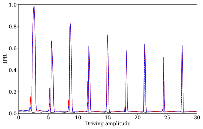
Figure 1: Plots of the two maximum IPR values (red solid and blue dashed lines) and minimum IPR value (black dash-dotted line) as a function of the driving amplitude $a$ in the range $[0,30]$. We see that states with maximum IPR $\gg 1/L$, called large-IPR states, appear in certain intervals of $a$. We have considered a 101-site system with $g=1$ and $\omega=1$.

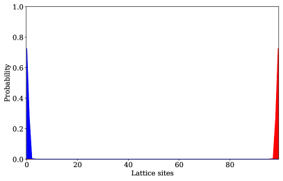
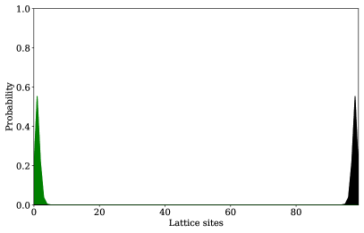
Figure 2: Four edge states for $a=5.6$ (type-1 region), for a 100-site system with $g=1$ and $\omega=1$.

Interestingly we see that the peaks in the IPR occur in the vicinity of the zeros of the Bessel function $J_{0}(a/\omega)$. An important thing to note is that in most of the regions where large-IPR states exist, there are four such states (two at each end of the system). These are the regions where both red and blue curves have large values; we will call these type-1 regions. The probabilities $|\psi(n)|^{2}$ for the four states are shown in Figs. 2 for a 100-site system with $g=1$, $\omega=1$ and $a=5.6$. The states shown in Figs. 2 (a) and (b) have somewhat different profiles, one of them being closer to the end than the other. There also exist small regions where only the red curve have a large value in Fig. 1; we call these type-2 regions. These regions are given by the intervals $[1.97,2.07]$, $[5.17,5.27]$, $[8.40,8.47]$, etc. In these regions, we have two large-IPR states, one at each end, if the number of sites $L$ is even, and one large-IPR state (which has a mode localized at each end simultaneously) if $L$ is odd. For a 100-site system with $g=1$, $\omega=1$, and $a=8.44$, we find that the probabilities for the edge states look very similar to the ones shown in Fig. 2 (a) and are therefore not shown here. The Floquet eigenvalues for $a=5.6$ (type-1) and $a=8.44$ (type-2) cases are shown in Figs. 3 and 4.

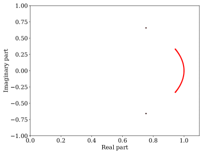
Figure 3: Plot of the real and imaginary parts of the Floquet eigenvalues $a=5.6$ (type-1 region), for a 100-site system with $g=1$ and $\omega=1$. There are four large-IPR states (shown in black) which are pairwise degenerate (hence we only see two black dots). These are well separated from the bulk states (shown by the red curve), and they correspond to bound states at the edges.

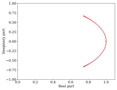
Figure 4: Plot of the real and imaginary parts of the Floquet eigenvalues for $a=8.44$ (type-2 region), for a 100-site system with $g=1$ and $\omega=1$. There are two large-IPR states (shown in black) whose eigenvalues lie close to 1. These lie within the bulk states (shown by the red curve), and they are not true edge states.

We find that there is a significant difference between the large-IPR states of type-1 and type-2. The type-1 states are exponentially localized at the edges; their wave functions go to zero rapidly as we go away from the edges; hence they are true edge states. (For example, for $g=1$, $\omega=1$ and $a=5.6$ which lies in the type-1 region, we find that for the edge states, the probability $|\psi(n)|^{2}$ in the middle of a 100-site system is only about $10^{-32}$ which is essentially zero). Hence their IPR remains large and constant as the system size is increased. This is shown in Fig. 5 for a system with $g=1$, $\omega=1$, and $a=5.6$ (type-1 region). The type-2 states have a large amplitude at the edges, but their wave functions approach some finite (although very small) values as we go away from the edges. Thus the type-2 states are not perfectly localized at the edges; they have a small but finite weight deep inside the bulk, even when the system size becomes very large. This difference in behavior is related to the following. We will see below that the Floquet eigenvalues of the type-1 edge states differ from those of the bulk states by a gap which remains finite as the system size $L\to\infty$. In contrast, the Floquet eigenvalues of the type-2 states lie in the middle of those of the bulk states; the gap between the eigenvalues of these large-IPR states and the bulk states goes to zero as the system size goes to infinity. We will see that the type-2 large-IPR states are actually made up of a linear combination of some bulk states.

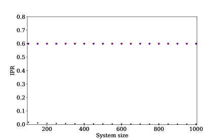
Figure 5: Plot of the largest two IPRs and the minimum IPR versus system size from $L=100$ to 1000 (in steps of 50), for $g=1$, $\omega=1$ and $a=5.6$ (type-1 region). The largest two IPRs correspond to the states at the two ends which are true edge states, hence the IPRs do not change with the system size. The minimum IPR corresponds to one of the bulk states.

We now present some numbers to provide a more detailed understanding of the large-IPR states which are actually not bound states at the edges. For convenience, we will discuss in this paragraph what happens if the phase of the hopping in Eq. (LABEL:ham4) is given by $\cos(\omega t)$ rather than $\sin(\omega t)$; then a Floquet eigenstate $\psi$ which exists at the left edge (starting at site $n=0$) will have $\psi(n)=0$ for all odd values of $n$ (see the discussion about symmetry in item (iii) below). It then turns out that we can tune one of the driving parameters (say, $a$) to find a value for which there is a state which is almost perfectly localized at one end of the system. For instance, for a 100-site system with $g=1$, $\omega=1$, we find that for $a=8.439$, there is a state which is large at the left end, with Floquet eigenvalue equal to 1 and IPR equal to $0.9982$. In this state, we find that the probabilities at the different sites are given approximately by $|\psi(0)|^{2}=0.9991$, $|\psi(2)|^{2}=8.2\times 10^{-4}$, $|\psi(4)|^{2}=1.8\times 10^{-6}$, $|\psi(6)|^{2}=|\psi(8)|^{2}=|\psi(10)|^{2}=\cdots=1.2\times 10^{-6}$, and $|\psi(n)|^{2}=0$ if $n$ is odd. The fact that the Floquet eigenvalue is equal to 1 implies that deep inside the bulk, this state must be a superposition of states with momenta $k=\pm\pi/2$, so that its energy is equal to $E_{k}=-2gJ_{0}(a/\omega)\cos k=0$ (see Appendix B). Next, we find that the above values of $|\psi(n)|^{2}$ remain unchanged even when $L$ is increased to, say, 1000. This can be understood as follows. The numerical program automatically normalizes the wave functions for a finite-sized system; hence for a system with $L$ sites and therefore $L/2$ even-numbered sites (we will assume that $L\gg 1$), the probabilities at the even-numbered sites are given by

$$(|\psi(0)|^{2},|\psi(2)|^{2},|\psi(4)|^{2},|\psi(6)|^{2},\cdots)$$

$$\simeq~{}\frac{1}{1+1.2\times 10^{-6}(L/2)}$$

$$~{}~{}\times~{}(0.9991,8.2\times 10^{-4},1.8\times 10^{-6},1.2\times 10^{-6},\cdots).$$

We then see that the probabilities at the first few sites will not change much from the values they have for $L=100$ till $L$ starts becoming comparable to $1/(1.2\times 10^{-6})\sim 10^{6}$. Clearly, one needs to go to enormous system sizes to distinguish between a true edge state (type-1) and a state which is not a bound state but has an IPR close to 1 when $L$ is about 100.

We thus conclude that periodic driving of a non-interacting tight-binding model with certain values of the driving amplitude $a$ can generate large-IPR states. These are bound states at the edges for type-1 but not true edge states for type-2 (although they can be made almost indistinguishable from a true edge state by tuning the driving parameters as we have seen above).

We will now discuss the symmetry properties of the Floquet operator $U_{T}$ which will, in turn, imply symmetries of the large-IPR states. The symmetries of $U_{T}$ follow from its definition as a time-ordered product (Appendix A). Using Eq. (LABEL:ham4), we can write the Hamiltonian $H$ for one particle as a $L\times L$ matrix in the basis of states $|n\rangle$ (which denotes the state where the particle is at site $n$). The symmetries of $U_{T}$ then follow from the symmetries of $H$ as follows.

(i) The fact that $\sin(\omega t)=-\sin(\omega(T-t))$ implies that $H^{*}(t)=H(T-t)$. This implies that $U_{T}^{*}=U_{T}^{-1}$. If $\psi$ is a Floquet eigenstate satisfying $U_{T}\psi=e^{i\theta}\psi$, this symmetry implies that $\psi^{*}$ is also a Floquet eigenstate with the same eigenvalue. We can then consider the superpositions $\psi+\psi^{*}$ and $i(\psi-\psi^{*})$ to show that $\psi$ can be chosen to be real.

(ii) If we combine the parity transformation $|n\rangle\to|L-1-n\rangle$ with $|n\rangle\to(-1)^{n}|n\rangle$ and complex conjugation, we find that $H(t)\to-H^{*}(t)$. This implies that $U_{T}$ is unitarily related to $U_{T}^{*}$. This implies that if $\psi(n)$ denotes the $n$-th component of an eigenstate of $U_{T}$ with eigenvalue $e^{i\theta}$, then a state $\psi^{\prime}$ with $\psi^{\prime}(n)=(-1)^{n}\psi^{*}(L-1-n)$ is an eigenstate of $U_{T}$ with eigenvalue $e^{-i\theta}$. This implies that if there is a Floquet eigenstate with a large weight near the left edge of the system with eigenvalue $e^{i\theta}$, there will be an eigenstate with a large weight near the right edge with eigenvalue $e^{-i\theta}$. It is clear that these two states have the same IPR since $\sum_{n=0}^{L-1}|\psi(n)|^{4}$ is invariant under $\psi(n)\to(-1)^{n}\psi(L-1-n)$.

(iii) If we shift the time $t\to t+T/4$, the term in the phase of the hopping amplitude in Eq. (LABEL:ham4) changes from $\sin(\omega t)$ to $\cos(\omega t)$. If we combine this with the transformation $|n\rangle\to(-1)^{n}|n>$, we have that $H(t)\to-H(T-t)$. More specifically, the transformation $|n\rangle\to(-1)^{n}|n\rangle$ is done by the unitary and diagonal matrix $W$ whose diagonal elements are given by $W_{nn}=(-1)^{n}$; since $W^{2}=I$, the eigenvalues of $W$ are equal to $\pm 1$. Then

$$WH(t)W~{}=~{}-~{}H(T-t),$$ (7)

and this implies that $WU_{T}W=U_{T}^{-1}$. Hence, for every Floquet eigenstate $\psi$ with eigenvalue $e^{i\theta}$, there will be an eigenstate $W\psi$ with eigenvalue $e^{-i\theta}$. We now recall that Floquet eigenvalues do not change under time shifts while eigenstates change by a unitary transformation; however, if there is a state with a large weight near one particular edge, its unitary transformation will give a state with a large weight at the same edge. We therefore conclude that near each edge, large-IPR states will either come in pairs with Floquet eigenvalues equal to $e^{\pm i\theta}$ (if $e^{i\theta}\neq\pm 1$), or they can come singly if the eigenvalue is equal to $\pm 1$. Further, the argument in the previous paragraph shows that there will be corresponding states with large weight at the opposite edge with the same eigenvalues. Also, if there is a single large-IPR state $\psi$ near an edge with Floquet eigenvalue equal to $\pm 1$, $W\psi$ will have the same eigenvalue and therefore must be identical to $\psi$ up to a sign. Hence $\psi$ must be an eigenstate of $W$. This means that the components of $\psi$, denoted as $\psi(n)$ must be zero if $n$ is odd (even) depending on whether $W\psi$ is equal to $+\psi$ or $-\psi$.

III.2 Tight-binding model with a staggered potential

We will now study the effects of a staggered potential $v$. The Hamiltonian with driving is given by

$$H = -~{}g~{}\sum_{n=0}^{L-2}~{}(e^{\frac{ia}{\omega}\sin(\omega t)}c_{n}^{\dagger}c_{n+1}~{}+~{}e^{-\frac{ia}{\omega}\sin(\omega t)}c_{n+1}^{\dagger}c_{n})$$ (8)

$$+~{}v~{}\sum_{n=0}^{L-1}~{}(-1)^{n}c_{n}^{\dagger}c_{n},$$

where $v$ is the strength of the staggered potential. The numerical results that we obtain are as follows. We have considered a 101-site system with $g=1$ and $\omega=1$. We then find that $v$ and $-v$ give identical plots for the IPRs. (We can show that the symmetry (ii) discussed above continues to hold if we also transform $v\to-v$, provided that $L$ is odd). We vary the driving amplitude $a$ from 0 to 30 in steps of $0.1$, and plot the largest two IPRs as a function of $v$. Figure 6 shows the IPRs for $v=\pm 1$. We find that large IPR values correspond to a pair of eigenstates which are localized at the opposite ends of the system and have the same Floquet eigenvalues. Since large values of IPRs imply the presence of edge states, we see that the regions where edge states exist are significantly larger compared to the case with $v=0$ (Fig. 1).

We can understand why the edge states at the opposite ends have the same Floquet eigenvalues as follows. When the number of lattice sites, $L$, is odd, the Hamiltonian and therefore the Floquet operator $U_{T}$ are invariant under a combination of parity ($n\to L-1-n$) and $a\to-a$. We have seen earlier that changing $a\to-a$ does not change the Floquet eigenvalues. The above symmetry therefore implies that if $\psi_{L}$ is a Floquet eigenstate localized near the left edge with a Floquet eigenvalue $e^{i\theta}$, there will be a Floquet eigenstate $\psi_{R}$ localized near the right edge with the same eigenvalue $e^{i\theta}$.

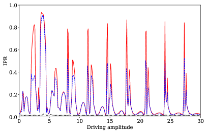
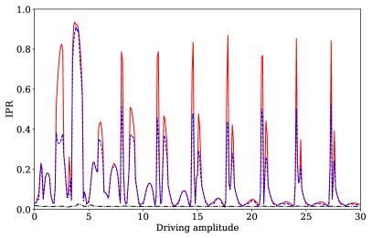
Figure 6: Largest two IPRs as a function of the driving amplitude $a$ for staggered potentials $v=1$ and $-1$, for a 101-site system with $g=1$ and $\omega=1$. The largest and second largest IPRs are shown as red solid and blue dashed lines. The smallest IPR is shown by a black dash-dotted line near the bottom. The two figures look identical due to a parity symmetry as discussed in the text.

There is an interesting difference between the cases where the number of sites is even and odd. In Fig. 7, we show the largest two eigenvalues for $v=\pm 1$ for a 100-site system in Fig. 7. We find once again that large values of the IPR correspond to a pair of eigenstates which are localized at opposite ends of the system; however their Floquet eigenvalues are complex conjugates of each other, unlike the case of an odd number of sites where the Floquet eigenvalues of the state at opposite ends are equal to each other.

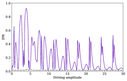
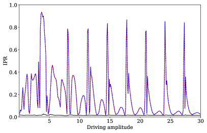
Figure 7: Largest two IPRs (which coincide with each other) as a function of the driving amplitude $a$ for staggered potentials $v=1$ and $-1$, for a 100-site system with $g=1$ and $\omega=1$. The smallest IPR is shown by a dash-dotted line near the bottom. The two figures are not identical as there is no parity symmetry when the number of sites is even.

In Fig. 8 we show the Floquet eigenvalues for a 100-site system with $g=1$, $\omega=1$, $v=1$ and $a=4$. The four isolated points correspond to edge states (two at each end). The value $a=4$ has been chosen since it corresponds to a peak in the largest two IPRs as shown in Fig. 7 (a).

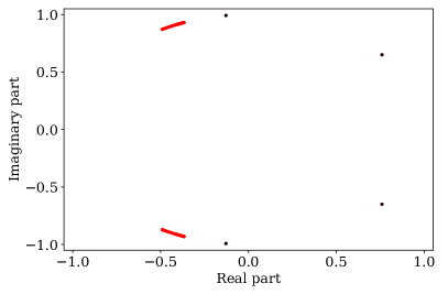
Figure 8: Plot of the real and imaginary parts of the Floquet eigenvalues for a 100-site system with $g=1$, $v=1$, $\omega=1$ and $a=4$. There are four large-IPR states (shown in black). These are well separated from the bulk states (shown by the red curves), and they correspond to bound states at the edges.

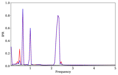
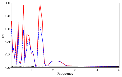
Figure 9: Largest two IPRs as a function of the driving frequency $\omega$ for staggered potentials $v=0$ and $1$, for a 101-site system with $g=1$ and $a=5.6$. The smallest IPR is shown by a black solid line near the bottom.

In Fig. 9 we show the largest two IPRs as a function of $\omega$ for a 101-site system with $g=1$ and $a=5.6$; we have taken $v=0$ and 1 in Figs. 9 (a) and (b) respectively. The figures show that edge states appear in a larger range of values of $\omega$ when $v$ is non-zero. However, edge states do not appear in either case when $\omega$ becomes large enough.

III.2.1 Floquet perturbation theory for $g\ll v$

We have seen numerically that the introduction of a non-zero $v$ enhances the regions of $a$ where edge states exist. We would now like to understand this analytically. Since we have taken the frequency $\omega$ to be of the same order as the hopping amplitude $g$, the Floquet-Magnus expansion in powers of $1/\omega$ would not be useful here bukov ; mikami . We will therefore use a different approach to understand the appearance of edge states. Namely, we will consider the limit $g\ll v$, and will use a Floquet perturbative expansion in $g$ to obtain a time-independent Hamiltonian. We will then match the results obtained in this way to those found numerically.

We begin by briefly discussing the Floquet perturbation theory soori ; bhaskar ; asmi . We write the Hamiltonian in Eq. (8) as $H=H_{0}+V$, where

$$H_{0} = v~{}\sum_{n=0}^{L-1}~{}(-1)^{n}c_{n}^{\dagger}c_{n},$$

$$V = -~{}g~{}\sum_{n=0}^{L-2}~{}[e^{\frac{ia}{\omega}\sin(\omega t)}c_{n}^{\dagger}c_{n+1}~{}+~{}e^{-\frac{ia}{\omega}\sin(\omega t)}c_{n+1}^{\dagger}c_{n}].$$

The eigenstates of $H_{0}$ are the states localized at various sites $|n\rangle=|0\rangle,|1\rangle,|2\rangle,\cdots$, and the eigenenergies are $E_{n}=+v$ or $-v$ depending on whether $n$ is even or odd. Now let $|\psi\rangle$ be a solution of the time-dependent Schrödinger equation. Then

$$i\frac{d\psi}{dt}~{}=~{}(H_{0}~{}+~{}V(t))~{}\psi.$$ (10)

We now write $\psi$ in terms of the eigenstates of $H_{0}$ as

$$|\psi(t)\rangle~{}=~{}\sum_{m}~{}c_{m}(t)~{}e^{-iE_{m}t}|n\rangle.$$ (11)

Substituting this in Eq. (10), we get an equation for the coefficients $c_{n}(t)$,

$$\frac{dc_{m}}{dt}~{}=~{}-i\sum_{m^{\prime}\neq m}\langle m|V(t)|m^{\prime}\rangle~{}e^{i(E_{m}-E_{m^{\prime}})t}~{}c_{m^{\prime}}(t).$$ (12)

We now solve Eq. (12) up to terms of order $g^{2}$. Integrating the above equation, we obtain

$$c_{m}(T)$$ (13)

$$= c_{m}(0)~{}-~{}i\sum_{m^{\prime}\neq m}\int_{0}^{T}dt\langle m|V(t)|m^{\prime}\rangle e^{i(E_{m}-E_{m^{\prime}})t}c_{m^{\prime}}(0)$$

$$-\sum_{m^{\prime}\neq m,m^{\prime\prime}}\int_{0}^{T}dt\langle m|V(t)|m^{\prime}\rangle e^{i(E_{m}-E_{m^{\prime}})t}$$

$$~{}~{}~{}\times\int_{0}^{t}dt^{\prime}\langle m^{\prime}|V(t^{\prime})|m^{\prime\prime}\rangle e^{i(E_{m^{\prime}}-E_{m^{\prime\prime}})t^{\prime}}c_{m^{\prime\prime}}(0).$$

We can re-write Eq. (13) as a matrix equation

$$c_{m}(T)e^{-iE_{m}T}~{}=~{}\sum_{m^{\prime}}(I~{}-~{}iTH_{F}^{(1)}~{}-~{}\dfrac{T^{2}}{2}H_{F}^{(2)})_{mm^{\prime}}c_{m^{\prime}}(0),$$ (14)

where $I$ is the identity matrix. We can now write the matrix appearing in Eq. (14) in the form

$$U_{eff}~{}=~{}e^{-iH_{eff}T}~{}\equiv~{}I~{}-~{}iTH_{F}^{(1)}~{}-~{}\dfrac{T^{2}}{2}H_{F}^{(2)}$$ (15)

up to order $T^{2}$. Namely, we have a unitary matrix $U_{eff}$ which is related to an effective Hamiltonian $H_{eff}$ which is correct up to order $g^{2}$. We find that $H_{eff}$ in terms $H_{F}^{(1)}$ and $H_{F}^{(2)}$ is

$$H_{eff}~{}=~{}H_{F}^{(1)}~{}+~{}\frac{iT}{2}~{}[H_{F}^{(2)}~{}-~{}(H_{F}^{(1)})^{2}].$$ (16)

We can now numerically compute the eigenvalues and eigenstates of $U_{T}=\mathcal{T}\exp(-i\int_{0}^{T}H(t)dt)$ and compare these with the same quantities for $U_{eff}$.

We note first that if $g=0$, the eigenstates of $U_{T}$ are just states localized at different lattice sites; there is a large degeneracy as states localized at even and odd number of sites have the same eigenvalues. With the introduction of even a small $g$, we see a drastic change in the eigenstates. For $g/v\simeq 1/100$ we find two localized edge states (one at each end) while all the other states are extended over the whole system. We find this numerically for both the periodically driven system ($U_{T}$) and the Floquet perturbative calculation ($U_{eff}$). For a 100-site system with $g=1$, $\omega=1$, $a=2.6$, and a large staggered potential $v=10.1$, we find that both $U_{T}$ and $U_{eff}$ have exactly two eigenstates localized at the edges (one at each edge), while all the other states are bulk states delocalized over the entire lattice. Further, the probabilities $|\psi(n)|^{2}$ for the edge states for $U_{T}$ and $U_{eff}$ look almost identical to each other (and are similar to the ones shown in Fig. 2 (a)).

To summarize this section, we see that the introduction of a small hopping $g$ in the driven system with a staggered potential $v$ can change the properties of the eigenstates significantly. We observe this numerically for both the driven system and the effective Hamiltonian obtained from Floquet perturbation theory.

III.2.2 Study of the maximum IPR versus $v$ for different values of $a$

We will now study the variation of the largest three IPRs as a function of $v$ for different values of $a$; this will give us information about the ranges of $v$ where localized edge states exist. In Fig. 10 we show the results for 100-site and 101-site systems, with $g=1$ and $\omega=1$. It is interesting to look at the point $v=0$. We see that the maximum IPR in the vicinity of $v=0$ is small for values of $a$, like $a=4$, which do not correspond to large IPR regions in Fig. 1, while it is large for values of $a$, like $a=2.6$, which lie in the large IPR region in Fig. 1. Hence the results for $v=0$ are consistent between Figs. 1 and 10. For larger values of $v$, we see sharp drops in the IPR values; this is due to hybridization between the edge states at the two ends of system which reduces their probabilities and therefore their IPRs.

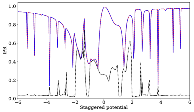
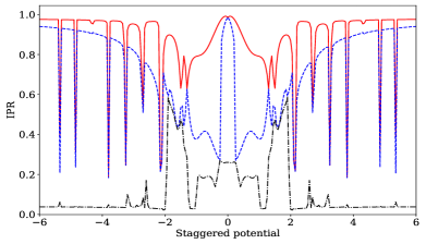
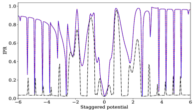
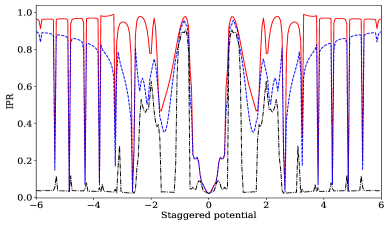
Figure 10: Largest three IPRs (shown as red solid, blue dashed and black dash dots, respectively) as a function of $v$ for different values of $a$ and number of sites, for $g=1$ and $\omega=1$. (a) $a=2.6$ and 100 sites, (b) $a=2.6$ and 101 sites, (c) $a=4$ and 100 sites, and (d) $a=4$ and 101 sites. The results are seen to depend on whether the number of sites is even or odd.

III.2.3 Time evolution of a state initialized at one edge

The driven system has another symmetry if the driving of the phase in Eq. (8) is taken to be $\cos(\omega t)$ instead of $\sin(\omega t)$. We then see that $H(T-t)=H(t)$. If we also change $v\to-v$ and $c_{n}\to(-1)^{n}c_{n}$, using the operator $W$ defined around Eq. (7), we have $H(T-t,-v)=-WH(t,v)W$. Following an argument similar to the one given there, we see that if $U_{T}(v)$ is the Floquet operator for a particular value of $v$, the Floquet operator for $-v$ is given by $U_{T}(-v)=W(U_{T}(v))^{-1}W$. Hence for every Floquet eigenstate of $U_{T}(v)$ given by $\psi(v)$ with Floquet eigenvalue $e^{i\theta}$, there will be a Floquet eigenstate of $U_{T}(-v)$ given by $\psi(-v)=W\psi(v)$ with Floquet eigenvalue $e^{-i\theta}$. Thus the results for $+v$ and $-v$ will be similar, and it is therefore sufficient to study the case $v\geq 0$. In the rest of this section, we will take the phase in Eq. (8) to be $\cos(\omega t)$.

We will now study the dynamics of states initialized near one edge of the system in the presence of periodic driving. We will start at time $t=0$ with a state which is localized at the left edge of the system and study how it evolves with time; the initial state will not be taken to be an eigenstate of the Floquet operator. We will look at how the probability that the particle returns to that edge (we will consider the first three sites to be the edge, so the edge probability is equal to $|\psi(0)|^{2}+|\psi(1)|^{2}+|\psi(2)|^{2}$) varies with the stroboscopic time which will be taken to be integer multiples of the time period $T$. We have studied a 100-site system with $g=1$, $\omega=1$, and $a=2.6$ (where we know that edge states exist for $v=0$) and $a=4$ (where there are no edge states for $v=0$). In Figs. 11 and 12, the sign of $v$ is the sign of the staggered potential at the first site from the left ($n=0$).

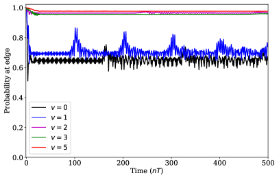
Figure 11: Edge probability of a state initialized at the left edge for a 100-site system with $g=1$, $\omega=1$, and $a=2.6$.

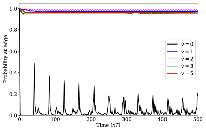
Figure 12: Edge probability of a state initialized at the left edge for a 100-site system with $g=1$, $\omega=1$, and $a=4$.

We conclude the following from Figs. 11 and 12.

(i) For $a=2.6$ where we know that edge states exist at $v=0$, the probability of staying at the edge remains close to 1 for all times. When $|v|$ is increased to 1 and 2, the probability becomes smaller. However, when $|v|$ is increased further to $3$ and $5$, the probability of staying at the edge again comes close to 1 at all times.

(ii) For $a=4$ where there is no edge state at $v=0$, the probability of staying at the edge remains close to zero, except for sharp peaks at some particular times. As $|v|$ is increased to 3 and 5, the probability rises and stays close to 1 at all times.

(iii) Even for values of $v$ and $a$ where the probability of staying close to the edge is small at most times, we see sudden jumps in the probability at some regular time intervals.

These features can be explained as follows. If the system has an edge state at a particular value of $a$ and $v$, then an initial state which is close to the edge will have a large overlap with that eigenstate and will therefore have a large probability for the particle to stay near the edge. This matches with our earlier plots showing the regions of $a$ and $v$ where edge states exist. When there are no edge eigenstates which are localized at the edges, the probability of staying near the edges is low. However there are peaks in the probability of coming close to the edge; this occurs because the particle initially starts at one edge, moves into the bulk, and then repeatedly gets reflected back and forth between the two edges. The probability becomes large whenever it returns to the original edge. This occurs at time intervals given by the recurrence time $2L/v_{max}$, where $L$ is the size of the system and $v_{max}$ is the maximum velocity of the particle when it is subjected to periodic driving. For instance, when the staggered potential $v=0$, the maximum velocity if $v_{max}=|2gJ_{0}(a/\omega)|$. This is because the effective Hamiltonian has a nearest-neighbor hopping amplitude equal to $-gJ_{0}(a/\omega)$ (see Appendix B). Hence the energy dispersion in the bulk is given by $E_{k}=-2gJ_{0}(a/\omega)\cos k$; the group velocity is then given by $v_{k}=2gJ_{0}(a/\omega)\sin k$, which has a maximum value of $|2gJ_{0}(a/\omega)|$.

IV Bose-Hubbard model with periodic driving

We will now consider a model with interacting particles. Specifically we will consider the Bose-Hubbard model and investigate if periodic driving can give rise to two-particle bound states which are localized at one edge of the system. On a lattice of size $L$, the Bose-Hubbard model subjected to periodic driving by an electric field has a Hamiltonian of the form

$$H = -~{}g~{}\sum_{n=0}^{L-2}~{}(e^{\frac{ia}{\omega}\sin(\omega t)}b_{n}^{\dagger}b_{n+1}~{}+~{}e^{-\frac{ia}{\omega}\sin(\omega t)}b_{n+1}^{\dagger}b_{n})$$ (17)

$$+~{}\frac{u}{2}~{}\sum_{n=0}^{L-1}\rho_{n}(\rho_{n}-1),$$

where $\rho_{n}=b_{n}^{\dagger}b_{n}$ is the particle number operator at site $n$. To study a system with two bosons numerically, we construct the Hamiltonian in the basis $|n_{1},n_{2}\rangle$, where $n_{1}$ and $n_{2}$ denote the positions of the two bosons, and we can assume that $n_{1}\leq n_{2}$ since the particles are indistinguishable. For a system with $L$ sites, the Hamiltonian in this basis will be a $L(L+1)/2$-dimensional matrix. After constructing the Hamiltonian we calculate the Floquet operator $U_{T}$ as explained in Appendix A. We then look at the Floquet eigenstates and their IPRs to identify bound states in which both the particles are localized near one edge of the system. In our calculations, we will define the edge as consisting of the three states $|0,0\rangle,~{}|0,1\rangle$ and $|1,1\rangle$, i.e., the probability at the edge will mean the sum of the probabilities of these states. In all our numerical calculations we will take $g=1$ and $\omega=1$, and vary the driving amplitude $a$ and the interaction strength $u$.

Before presenting the numerical results, we note a useful symmetry which relates the Floquet operators for positive and negative values of $u$. This can be seen most clearly if we take the phase of the hopping to be $\cos(\omega t)$ instead of $\sin(\omega t)$ in Eq. (17); then the symmetry $\cos(\omega(T-t))=\cos(\omega t)$ implies that the Hamiltonian $H(t)\to-H(T-t)$ if we change $u\to-u$ and $b_{n}\to(-1)^{n}b_{n}$. The latter corresponds to a transformation by a unitary and diagonal matrix $W_{2}$ which gives $W_{2}|n_{1},n_{2}\rangle=(-1)^{n_{1}+n_{2}}|n_{1},n_{2}\rangle$; note that $W_{2}^{2}=I$. This implies that the Floquet operators for interaction strengths $\pm u$ are related as $U_{T}(-u)=W_{2}(U_{T}(u))^{-1}W_{2}$. Hence, if there is a two-particle bound state $\psi(u)$ at one edge of the system with a Floquet eigenvalue $e^{i\theta}$ for interaction $u$, there will be a two-particle bound state $\psi(-u)$ at the same edge with a Floquet eigenvalue $e^{-i\theta}$ for interaction $-u$; the wave functions for the two eigenstates will be related as $\psi(-u)=W_{2}\psi(u)$. This implies that the probabilities of the different basis states $|n_{1},n_{2}\rangle$ will be identical in the two eigenstates. This symmetry between positive and negative values of $u$ implies that it is sufficient to study the case $u\geq 0$.

IV.1 Edge probability versus $u$ for different values of $a$

We recall from Fig. 1 that driving the non-interacting model with $a=2.6$ gives rise to edge states, while $a=4$ does not lead to edge states. To study the possibility of interactions producing two-particle bound states which are localized near one of the edges, we will specifically choose these two values of $a$ and study the probability at the edge as a function of the interaction strength $u$; we define the edge probability to be the sum of the probabilities of the two particles being at the locations $|0,0\rangle$, $|0,1\rangle$ and $|1,1\rangle$. The numerical results obtained for a 30-site system are shown in Fig. 13. We note the following features in the figure.

(i) For $a=2.6$, the edge probability is fairly large at $u=0$. This is because the non-interacting system has edge states as we saw in Fig. 1, and therefore there are states in which both the particles occupy those states. However, as $u$ is turned on, either to positive or negative values, the edge probability first drops and then starts rising again with increasing $u$. Thus a two-particle bound state at the edge becomes more likely as $u$ increases.

(ii) For $a=4$, the edge probability is small at $u=0$; this is because the non-interacting system does not have edge states as shown in Fig. 1. As $u$ is turned on, the probability at the edge first rises, then drops and then starts rising again as $u$ increases.

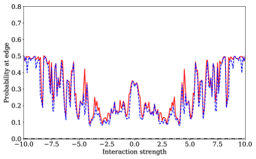
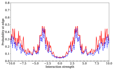
Figure 13: Largest two edge probabilities at edge as a function of $u$. For $a=2.6$, $u=0$ gives a large probability at the edge, while for $a=4$, $u=0$ gives an edge probability close to 0. The overall trend is that as $u$ increases the edge probability increases. Note that a large edge probability does not necessarily imply a bound state.

IV.2 Floquet perturbation theory for $g\ll u$

We now present a Floquet perturbation theory in the limit that $g\ll u$ along the same lines as in Sec. III.2.1. We write the Hamiltonian as a sum

$$H = H_{0}+V,$$

$$H_{0} = \frac{u}{2}~{}\sum_{n=0}^{L-1}~{}\rho_{n}(\rho_{n}-1),$$

$$V = -~{}g~{}\sum_{n=0}^{L-2}~{}(e^{\frac{ia}{\omega}\sin(\omega t)}b_{n}^{\dagger}b_{n+1}~{}+~{}e^{-\frac{ia}{\omega}\sin(\omega t)}b_{n+1}^{\dagger}b_{n}),$$

and treat $V(t)$ as a perturbation. We first consider the limit $g=0$, so the Hamiltonian is $H_{0}=(u/2)\sum_{n=0}^{L-1}\rho_{n}(\rho_{n}-1)$. Then the eigenstates of the Hamiltonian are simply the basis states $|n_{1},n_{2}\rangle$, and driving has no effect on this system. We now find that introducing even a small amount of hopping ($g\ll u$) has a drastic effect. Namely, we find that all bulk states are delocalized and there are only two two-particle bound states which are localized at one of the ends of the system. We can use Floquet perturbation theory to first order in $g$ to understand the emergence of two-particle edge states for small hopping. Before showing the results we first discuss Floquet perturbation theory for this system. For convenience, we will denote the eigenstates of $H_{0}$, $|n_{1},n_{2}\rangle$ by a single symbol $|m\rangle$, where $m$ takes $L(L+1)/2$ possible values. The eigenenergies of $H_{0}$ are $E=0$ or $u$ depending on whether the two bosons are on the same site or on different sites. Since there are degeneracies in the eigenenergies of $H_{0}$, we have to use degenerate Floquet perturbation theory. We look for solutions of the time-dependent Schrödinger equation $|\psi\rangle$ for the time-periodic Hamiltonian $H$. We can write

$$|\psi(t)\rangle=\sum_{m}c_{m}(t)e^{-iE_{m}t}|m\rangle.$$ (19)

Then the Schrödinger equation leads to the following equations for the amplitudes $c_{m}(t)$,

$$\frac{dc_{m}}{dt}~{}=~{}-i\sum_{m^{\prime}\neq m}\langle m|V(t)|m^{\prime}\rangle e^{i(E_{m}-E_{m^{\prime}})t}~{}c_{m^{\prime}}(t).$$ (20)

Up to first order in $g$ and $T$, the effective time-evolution operator relating $c_{m}(T)e^{-iE_{m}T}$ to $c_{m}(0)$ is then given by

$$U_{eff}~{}=~{}I~{}-~{}iTH_{F}^{(1)},$$ (21)

where

$$(H_{F}^{(1)})_{mm^{\prime}}$$

$$= (H_{0})_{mm^{\prime}}~{}+~{}\dfrac{1}{T}~{}\int_{0}^{T}dt~{}e^{i(E_{m}-E_{m^{\prime}})t}~{}\langle m|V(t)|m^{\prime}\rangle.$$

We will now show a comparison of the numerical results obtained for the driven system and those obtained from the effective Hamiltonian $H_{F}^{(1)}$ obtained from Floquet perturbation theory. We consider a $30$-site system with $g=0.1$, $u=20.2$ and $\omega=1$, so that $g\ll u$. We have shown the results for $a=2.6$ in Figs. 14 and 15. In Fig. 14 we see two states with large IPRs which are two-particle bound states localized at one of the two ends of the system. The probabilities $|\psi(n_{1},n_{2})|^{2}$ of these states are shown in Figs. 15 (a-d). We find a good match between the results obtained numerically (Figs. 15 (a) and 15 (c)) and perturbatively (Figs. 15 (b) and 15 (d)).

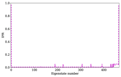
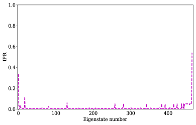
Figure 14: Comparison between IPR plots for the driven system and the perturbatively obtained Hamiltonian respectively for a 30-site system with $g=0.1$, $u=20.2$, $\omega=1$, and $a=2.6$. The IPR plots show two states with large IPRs implying a localized bound state at each of the edges.

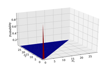
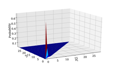
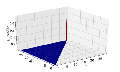
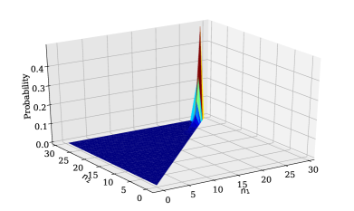
Figure 15: Comparison between numerical results for the driven system and the perturbatively obtained Hamiltonian respectively for a 30-site system with $g=0.1$, $u=20.2$, $\omega=1$, and $a=2.6$. The two-particle probability $|\psi(n_{1},n_{2})|^{2}$ vs $(n_{1},n_{2})$, where $n_{1}\leq n_{2}$, obtained numerically and perturbatively are shown for the two states in plots (a), (c) and (b), (d) respectively.

IV.3 Time evolution of a two-particle state initialized at one edge

We will now study the time evolution of the probability of two particles remaining close to the edge where they are initialized. We will take the initial state to be one where both particles are at the site labeled 0. We define the probability of the two particles to remain near the edge as the sum $|\psi(0,0)|^{2}+|\psi(0,1)|^{2}+|\psi(1,1)|^{2}$ and track this as a function of time. We study this for different values of the driving amplitude $a$ and the interaction strength $u>0$. We again choose two values of $a$ given by $2.6$ and $4$, one lying within the region where single-particle edge states exist, and one lying in the region where there are no edge states. We consider a 20-site system with $g=1$ and $\omega=1$. The numerical results are shown in Figs. 16 and 17 for $a=2.6$ and 4 respectively. We note the following.

(i) For $a=2.6$ where the non-interacting driven model hosts edge states, we see that for $u=0$ the particle always stays near the edge, hence the probability remains non-zero for all times. For $a=4$ which does not give edge states when driven, the probability for $u=0$ drops to zero quickly. Thus the two bosons quickly spread out into the bulk of the system.

(ii) For a moderately strong interaction strength $u=\pm 2,~{}\pm 4$ (of the same order as the hopping $g$), the probability to remain at the edge remains small for all times. Hence a moderate amount of either attraction or repulsion makes the bosons delocalize into the bulk.

(iii) For large $u=\pm 10,~{}\pm 20$ the two particles remain localized near the edge for all times. For large and attractive $u$ this is easy to understand as the two particles being at the zeroth site form a deep attractive well leading to a bound state. This is also true for large and repulsive $u$ since the particles form a deep repulsive well which leads to a bound state on a lattice. (It is interesting to note, for instance, that a large attractive or repulsive potential at one site on a lattice can host a bound state localized near that site, whereas in a continuum model, a $\delta$-function potential can host a bound state only if it is attractive). Hence a small hopping ($g\ll|U|$) cannot delocalize the two bosons for either sign of $u$.

(iv) An interesting feature in some of the plots is the oscillation of the probability with a large time period for certain parameter values. For instance, for $a=2.6$ this happens for $u=\pm 6$ as we see in Fig. 16. This can be understood as follows. If there are two Floquet eigenstates which are localized at the edge, have slightly different Floquet eigenvalues, and have a large overlap with the initial state where both particles are at the zeroth sites, then the time-evolved state will oscillate back forth with a time period with is inversely proportional to the difference of the quasienergies of the two bound state. Indeed we find that for the parameter values given above there are two such eigenstates at the edge with closely spaced Floquet eigenvalues.

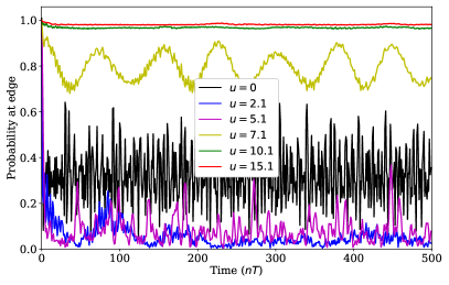
Figure 16: Return probability of a state initialized with both particles at left edge. We have taken a 20-site system with $a=2.6$ and $g=1$.

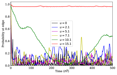
Figure 17: Return probability of a state initialized with both particles at edge. We have taken a 20-site system with $a=4$ and $g=1$.

V Detection of edge states using transport measurements

In this section we will discuss how it may be possible to detect the edge states studied in the earlier sections by looking at transport across the driven system. In particular, if one attaches metallic leads to the two ends of the system, we find that signatures of the edge states may appear as peaks in the differential conductance when one applies a voltage bias across the system which is equal to the quasienergy of one of the edge states. To find the differential conductance across a periodically driven system we have to calculate use Floquet scattering theory moskalets ; agarwal .

Floquet scattering theory works most easily if we consider a model without interactions. We will consider a system of non-interacting electrons described by the driven tight-binding system discussed in Sec. III, which is attached to two leads which are not driven. We will ignore the spin of the electron in this section; to include the effect of spin we will only need to multiply our final results for the conductance by a factor of 2. The Hamiltonian of our system will have the following parts. The periodically driven part in the middle (called the wire $W$) will have $L$ sites going from $n=0$ to $L-1$; the Hamiltonian in this region will be

$$H_{W}~{}=~{}-~{}g~{}\sum_{n=0}^{L-2}~{}(e^{i\frac{a}{\omega}\sin(\omega t)}c_{n}^{\dagger}c_{n+1}~{}+~{}e^{-i\frac{a}{\omega}\sin(\omega t)}c_{n+1}^{\dagger}c_{n}).$$ (23)

(We will ignore the staggered potential $v$ in this section). The leads on the left and right sides of the wire, $L$ and $R$, consist of sites from $n=-\infty$ to $-1$ and from $n=L$ to $\infty$ respectively, with the Hamiltonians

$$H_{L} = -~{}g_{l}~{}\sum_{n=-\infty}^{-2}~{}(c_{n}^{\dagger}c_{n+1}+c_{n+1}^{\dagger}c_{n}),$$

$$H_{R} = -~{}g_{l}~{}\sum_{n=L}^{\infty}(c_{n}^{\dagger}c_{n+1}+c_{n+1}^{\dagger}c_{n}).$$ (24)

(Note that the energy bands in the wire and leads will lie in the ranges $[-2g,2g]$ and $[-2g_{l},2g_{l}]$, respectively, and we are allowing these to differ from each other). Finally, there will be couplings between the left and right leads and the wire given by the Hamiltonian

$$H_{C}~{}=~{}-~{}g_{c}~{}(c_{-1}^{\dagger}c_{0}~{}+~{}c_{0}^{\dagger}c_{-1}~{}+~{}c_{L-1}^{\dagger}c_{L}~{}+~{}c_{L}^{\dagger}c_{L-1}).$$ (25)

We will now consider an electron which is incident from the left lead with an energy $E_{0}=-2g_{l}\cos(k_{0})$ and wave function $\psi(n)=e^{i(k_{0}n-E_{0}t)}$; the energy must lie in the range $[-2g_{l},2g_{l}]$. When the electron enters the wire region which is being driven with a frequency $\omega$, it may lose or gain energy in multiples of $\omega$. Hence it may get reflected back to the left lead or transmitted to the right lead with an energy $E_{p}=E_{0}-p\omega$, where $p$ is an integer. This must be related to the momentum $k_{p}$ by the relation $E_{p}=-2g_{l}\cos(k_{p})$. For this to describe a propagating wave, we must have $k_{p}$ real which means that $E_{p}$ must lie in the range $[-2g_{l},2g_{l}]$. If $E_{p}$ lies outside this range, the corresponding wave functions $e^{ik_{p}n}$ should decay exponentially as we go away from the wire into the leads; hence $k_{p}$ will be complex and we have to choose the imaginary part of $k_{p}$ appropriately. We find that $k_{p}$ has to be chosen as follows.

(i) For $-2g_{l}\leq E_{p}\leq 2g_{l}$, we have $k_{p}=\cos^{-1}[-E_{p}/(2g_{l})]$, and we choose $0\leq k_{p}\leq\pi$. The group velocity for this case is given by $v_{p}=dE_{p}/dk_{p}=2g_{l}\sin(k_{p})$ which satisfies $v_{p}\geq 0$. This will appear in the expressions for the currents in the leads.

(ii) For $E_{p}<-2g_{l}$, we have $k_{p}=i\cosh^{-1}(-\frac{E_{p}}{2g_{l}})$. This corresponds to a decaying wave function which does not contribute to the current in the leads.

(iii) For $E_{p}>2g_{l}$, we have $k_{p}=i\cosh^{-1}(\frac{E_{p}}{2g_{l}})+\pi$. This also corresponds to a decaying wave function and does not contribute to the current.

Next, we find the reflection and transmission amplitudes, $r_{p}$ back to the left lead and $t_{p}$ to the right lead respectively, for different values of $E_{p}$. To do this, we write down the wave functions in the wire and the leads and use their continuity at the junctions between the different regions. The wave functions are as follows.

(i) Region I (left lead):

$$\psi(n) = e^{i(k_{0}n-E_{0}t)}$$ (26)

$$+~{}\sum_{p=-\infty}^{\infty}r_{p}~{}e^{i(-k_{p}n-E_{p}t)}~{}~{}~{}{\rm for}~{}~{}~{}n\leq-1.$$

(ii) Region II (wire):

$$\psi(n)~{}=~{}\sum_{p=-\infty}^{\infty}c_{n,p}~{}e^{-iE_{p}t}~{}~{}~{}{\rm for}~{}~{}~{}0\leq n\leq L-1.$$ (27)

(iii) Region III (right lead):

$$\psi(n)~{}=~{}\sum_{p=-\infty}^{\infty}t_{p}~{}e^{i(k_{p}n-E_{p}t)}~{}~{}~{}{\rm for}~{}~{}~{}n\geq L.$$ (28)

We now solve the Schrödinger equation $id\psi/dt=H\psi$, where $\psi$ denotes all the $\psi(n)$’s combined into a column, and the Hamiltonian $H$ in this equation can be obtained from the second-quantized Hamiltonians in Eqs. (23-25) in the usual way. Solving these equations, which naturally involves matching the wave functions at the junctions between the different regions, and equating the coefficients of $e^{-iE_{p}t}$ on the two sides of every equation for all values of $p$, we obtain the following $L+2$ equations for each value of $p$,

$$g_{c}~{}c_{0,p}~{}-~{}g_{l}~{}r_{p}~{}=~{}g_{l}~{}\delta_{p,0},$$

$$g_{c}~{}r_{p}~{}e^{ik_{p}}~{}+~{}E_{p}~{}c_{0,p}$$

$$+~{}g~{}\sum_{m=-\infty}^{\infty}J_{m}(a/\omega)~{}c_{1,p+m}~{}=~{}-g_{c}~{}e^{-ik_{0}}~{}\delta_{p,0},$$

$$g~{}\sum_{m}(-1)^{m}J_{m}(a/\omega)~{}c_{n-1,p+m}~{}+~{}E_{p}~{}c_{n,p}$$

$$+~{}g~{}\sum_{m}J_{m}(a/\omega)~{}c_{n+1,p+m}~{}=~{}0~{}~{}~{}{\rm for}~{}~{}~{}1\leq n\leq L-2,$$

$$g~{}\sum_{m}(-1)^{m}J_{m}(a/\omega)~{}c_{L-2,p+m}~{}+~{}E_{p}~{}c_{L-1,p}$$

$$+~{}g_{c}~{}t_{p}~{}e^{ik_{p}L}~{}=~{}0,$$

$$g_{c}~{}c_{L-1,p}~{}-~{}g_{l}~{}t_{p}~{}e^{ik_{p}(L-1)}~{}=~{}0.$$ (29)

We can write Eqs. (29) as a matrix equation where the left-hand side consists of a matrix acting on a column of $r_{p},~{}t_{p}$ and $c_{n,p}$’s, and the right-hand side is given by a column formed out of the right-hand sides of the same equations. Inverting this matrix equation we can obtain the $r_{p},t_{p}$ and $c_{n,p}$’s in principle. However, this is a infinite-dimensional matrix equation and we must therefore truncate it to find the solutions numerically. If we keep only $2n_{H}+1$ values of $p$, going from $p=-n_{H}$ to $+n_{H}$, we will obtain a $(L+2)(2n_{H}+1)$-dimensional matrix from which we can find $r_{p},t_{p}$ and $c_{n,p}$. To see if the truncation error is small enough, we can verify how well the current conservation relation

$$v_{0}=\sum_{p}~{}v_{p}~{}(|r_{p}|^{2}+|t_{p}|^{2})$$ (30)

is satisfied, where $v_{p}$ is the group velocity for energy $E_{p}$, and the sum over $p$ in Eq. (30) only runs over values for which $E_{p}$ lies in the range $[-2g_{p},2g_{p}]$.

In the above analysis, we have assumed that the electron is incident from the left lead with an energy $E_{0}$. We can similarly consider what happens if an electron is incident from the right lead with the same energy $E_{0}$. We denote the corresponding reflection and transmission amplitudes by $r_{p}^{\prime}$ back to the right lead and $t_{p}^{\prime}$ to the left lead respectively. We now note that the Hamiltonians in Eqs. (23-25) have a parity symmetry if we shift $t\to t+\pi/\omega$ (this interchanges the factors of $e^{\pm i(a/\omega)\sin(\omega t})$ appearing in Eq. (23)). Hence we will have $|t_{p}|^{2}=|t_{p}^{\prime}|^{2}$ and $|r_{p}|^{2}=|r_{p}^{\prime}|^{2}$. This implies that the outgoing current in the right lead will be given by moskalets

$$I_{R}~{}=~{}\frac{e}{h}\int_{-2g_{l}}^{2g_{l}}~{}dE_{0}~{}\sum_{p=-\infty}^{\infty}\frac{v_{p}}{v_{0}}~{}|t_{p}|^{2}~{}[f(_{L}(E_{0})~{}-~{}f_{R}(E_{0})],$$ (31)

where $f_{L/R}(E_{0})=[e^{(E_{0}-\mu_{L/R})/(k_{B}T)}+1]^{-1}$ denotes the Fermi-Dirac functions for the left (right) leads respectively, the chemical potentials are $\mu_{L/R}=-eV_{L/R}$ where $V_{L/R}$ denote the voltages applied to the leads, $-e$ denotes the electron charge, $h=2\pi\hbar$, and we have ignored the electron spin in writing Eq. (31). At zero temperature ($T=0$), we get $I_{R}=0$ if $V_{L}=V_{R}$. If we set $V_{R}=-E_{0}/e$ and take the limit $V_{L}\to V_{R}$, the differential conductance $G=I_{R}/(V_{L}-V_{R})$ is given by

$$G~{}=~{}\frac{e^{2}}{h}~{}\sum_{p}~{}\frac{v_{p}}{v_{0}}~{}|t_{p}|^{2},$$ (32)

where $|t_{p}|^{2}$ is evaluated at the energy $E_{0}$. We can now plot $G$ as a function of $E_{0}$ to see if any peaks appear due to the edge states produced by the driving in the wire region.

We will now present our numerical results for the edge states and their effects in a plot of $G$ versus of $E_{0}$ in Figs. 18 and 19. We take the coupling between the wire and the leads to be small, i.e., $g_{c}\ll g_{l}$, so that the edge states are not significantly disturbed by this coupling. We choose $g=g_{l}=1$, $g_{c}=0.01$ and $\omega=\pi/4$, and consider two values of $a/\omega=2.5$ and $5.6$ where we know that edge states exist. We indeed see that there are peaks when $E_{0}$ is equal to the quasienergy of any of the edge states or $E_{0}$ differs from the quasienergies by integer multiples of $\omega$. In general we also find contributions to $G$ from the bulk states in the wire, but in the limit $g_{c}\ll g$, these vanish, and we only see contributions from the edge states. It is important to note here that although the band width in the leads, $4g_{l}$, is equal to the bare band width in the wire, $4g$, the driving reduces the effective band width in the wire to $4g|J_{0}(a/\omega)|$, as explained in Appendix B (for $a/\omega=2.5$ and $5.6$, $|J_{0}(a/\omega)|=0.048$ and $0.027$ respectively). As a result, we have edge states whose Floquet eigenvalues lie well outside the effective band width of the wire but inside the band width of the leads. This makes it possible to detect these edge states by sending in an electron with the appropriate energy from the leads, while easily distinguishing their contributions from those of the bulk states in the wire.

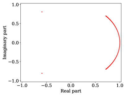
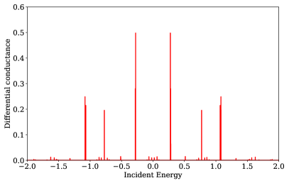
Figure 18: (a) Floquet eigenvalues of edge states (isolated red dots): $-0.5925\pm 0.8056i$ corresponding to quasienergy = $\pm 0.2756$. (b) We see peaks in the differential conductance $G$ (in units of $e^{2}/h$) when the incident electron has the same energy. The other peaks in $G$ correspond to side bands with energies equal to $\pm 0.2756\pm p\omega$.

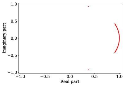
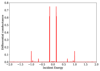
Figure 19: (a) Floquet eigenvalues of edge states (isolated red dots): $0.3755\pm 0.9268i$ corresponding to quasienergy = $\pm 0.1482$. (b) We see peaks in the differential conductance $G$ (in units of $e^{2}/h$) when the incident electron has the same energy. The other peaks in $G$ correspond to side bands with energies equal to $\pm 0.1482\pm p\omega$

Figure 18 (a) shows that the Floquet eigenvalues for a driven 100-site system (with no leads) for $g=1$, $\omega=\pi/4$, and $a/\omega=2.5$. The edge states are clearly distinguishable from the bulk states; their Floquet eigenvalues are $-0.5925\pm 0.8056i$, and the the corresponding quasienergies are $\pm 0.2756$. To calculate the differential conductance, we have chosen a smaller system with $L=10$, so that the states at the two edges can hybridize with each other and thereby lead to transmission across the wire. We choose $g=g_{l}=1$ and $g_{c}=0.01$; the small values of $g_{c}$ (which is equivalent to having a large barrier between the wire and the leads) ensures that the bulk states in the wire contribute very little to the conductance. Figure 18 (b) shows a plot of $G$ versus $E_{0}$. We see that there are exactly at the quasienergies $\pm 0.2756$ corresponding to the edge states and also at side bands whose energies differ from the edge states by integer multiples of $\omega$.

In Figs. 19 (a) and (b), we show the same results for $a/\omega=5.6$; all the other parameters have the same values as in Figs. 18. The edge states now have Floquet eigenvalues $0.3755\pm 0.9268i$, corresponding to quasienergies $\pm 0.2756$. Once again we see peaks in $G$ at these quasienergies and other energies differing from them by integer multiples of $\omega$.

We emphasize that the detection of edge states through a measurement of the conductance requires that the states at the two edges must hybridize with each other by a significant amount; if they do not hybridize, the electron will not be transmit from one end to the other. The hybridization between the two edges is crucially dependent on the system size $L$. We find numerically that the hybridization becomes very small beyond about $L=20$ for the parameter values that we have chosen. This is because the wave function decreases exponentially with some decay length as we go away from the edge; hence the overlap between the edge states at the two ends will become very small if $L$ becomes larger than the decay length. Figure 20 shows a plot of the maximum value of $G$ (i.e., maximized as a function of the incident energy) versus the system size $L$, for the same parameter values as in Figs. 18. We see that there is a sharp drop beyond about $L=20$.

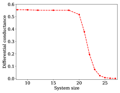
Figure 20: Maximum differential conductance $G$ (in units of $e^{2}/h$) versus system size $L$. We have chosen $\omega=\pi/4$, $a/\omega=2.5$ (so that $J_{0}(a/\omega)$ is close to zero), $g=g_{l}=1.0$, and $g_{c}=0.01$

VI Discussion

We begin by summarizing our results. We find that a tight-binding model in one dimension can host edge states when the phase of the hopping amplitude is periodically driven in time by applying an oscillating electric field. The presence of a staggered potential or an on-site Bose-Hubbard interaction generally enhances the regions where such states appear. The edge states only appear when the driving frequency is of the order of the hopping. For frequencies much larger than the hopping, we find that there are no edge states; the reason for this is explained at the end of Appendix C 1. Hence we cannot use the Floquet-Magnus expansion bukov ; mikami , which is valid at high frequencies, to study the edge states. We have used a Floquet perturbation theory to show that when the staggered potential or the interaction strength is much larger than the hopping, periodic driving can generate states localized at the edges. The results obtained by this method agree well with those found numerically. Finally, we have shown that a measurement of the differential conductance across a periodically driven wire with non-interacting electrons can detect the edge states; the conductance has peaks when the voltage bias coincides with the quasienergy of one of the edge states.

We now recall our most interesting findings. In the case of a non-interacting model, we have studied the ranges of the various parameters for which one or more Floquet eigenstates exist near each edge of a long but finite system. In some cases, we find that these states are truly localized at the edges; their wave functions decay rapidly to zero as one moves away from the edges and are therefore normalizable. In other cases, we find that the wave functions are much larger at the edges than in the bulk; however, they do not go to zero as we go deep into the bulk, and the wave functions are therefore not normalizable. (By tuning the driving parameters, however, the wave functions of these states can be made to go to almost zero in the bulk and therefore look very similar to true edge states). We find that the two kinds of states are respectively associated with Floquet eigenvalues which lie outside or within the continuum of eigenvalues of the bulk states. We have then studied the time evolution of a state which is not a Floquet eigenstate and is initially localized at the edge of the system. Depending on the system parameters, we find that the state can, with a finite probability, remain localized near the edge for all times or can move away completely into the bulk. The former happens if the system has Floquet eigenstates which are localized at the edges. A similar phenomenon occurs in the periodically driven Bose-Hubbard model with two particles when we study the time evolution of a state which initially has both particles at the edge. Once again we find that the particles can remain at the edge with a finite probability or move away into the bulk, depending on the system parameters, and the former happens if there are Floquet eigenstates which are localized at the edges. At the end, we have studied how the edge states can be detected using transport measurements. We consider a tight-binding model of non-interacting fermions in which semi-infinite leads are weakly coupled to a finite length wire in the middle. The hopping phase is periodically driven in the wire; this effectively reduces the value of the hopping in the wire and this can make the band width in the wire much smaller than in the leads. We find that when the isolated wire (i.e., without any leads) has edge states whose Floquet eigenvalues lie outside the range of eigenvalues of the bulk states of the wire, the differential conductance across the system with leads has peaks when the chemical potential of the leads is equal to the quasienergies of the edge states. Hence the conductance can provide clear evidence of the presence of edge states.

We would like to point out two directions for detailed investigations in the future. First, we do not know if the edge states have a topological significance. There does not seem to be a topological invariant which can tell us how many such states should appear at each edge for a given set of system parameters. Second, it would be interesting to examine the effects of disorder on the various edge states. We have found that the edge states are robust to some amount of disorder if their Floquet eigenvalues are separated by a gap from the eigenvalues of the bulk states. This gap-induced protection has been found in other driven systems as well deb ; saha .

It may be possible to test the results presented in this paper in systems of cold atoms trapped in an optical lattice which is periodically shaken eckardt ; lignier . In such systems, the driving parameters can be experimentally varied over a wide range which would allow one to change the ratio $a/\omega$ across several zeros of the Bessel function as in Fig. 1. Regarding the Bose-Hubbard model, the on-site two-body interaction $U$ can be modulated by magnetic Feshbach resonance chin . There are experiments on static systems where the ratio $U/g$ could be varied over a large range trotzky . Periodic driving of such a system would allow one to test our results for this model. Finally, transport measurements for detecting the edge states can be carried out in quantum wire systems where a portion of the wire is subjected to electromagnetic radiation which is associated with an oscillating electric field.

Acknowledgments

S.S. thanks MHRD, India for financial support through a PMRF. D.S. thanks DST, India for Project No. SR/S2/JCB-44/2010 for financial support.

Appendix A Basics of Floquet theory

In this Appendix we will briefly present the basics of Floquet theory bukov ; mikami . Consider a time-periodic Hamiltonian with period $T$, so $H(t+T)=H(t)$. According to Floquet theory, the solutions $\psi_{n}(t)$ of the time-dependent Schrödinger equation $id\psi_{n}/dt=H\psi_{n}$ can be taken to satisfy the condition

$$\psi_{n}(T)~{}=~{}e^{-i\epsilon_{n}T}\psi_{n}(0),$$ (33)

where $e^{-i\epsilon_{n}T}$ is the $n$-th Floquet eigenvalue and $\psi_{n}(0)$ is the corresponding Floquet eigenstate. The quantity $\epsilon_{n}$ is called the quasienergy. Since changing $\epsilon\to\epsilon+j\omega$, where $\omega=2\pi/T$ and $j$ can be any integer, does not change the value of $e^{-i\epsilon T}$, we can take $\epsilon_{n}$ to lie in the range $[-\omega/2,\omega/2]$. Next, we can write $\psi_{n}(t)$ in the form

$$\psi_{n}(t)~{}=~{}e^{-i\epsilon_{n}t}~{}\sum_{m=-\infty}^{\infty}~{}e^{-im\omega t}\phi_{n,m}.$$ (34)

Similarly, the time-periodic Hamiltonian can be written as

$$H~{}=~{}\sum_{p=-\infty}^{\infty}~{}e^{-ip\omega t}H_{p},$$ (35)

Substituting the above expressions in the Schrödinger equation, we obtain an infinite set of equations shirley

$$\sum_{p=-\infty}^{\infty}~{}H_{p}~{}\phi_{n,m-p}~{}=~{}(\epsilon_{n}~{}+~{}m\omega)~{}\phi_{n,m},$$ (36)

where $m$ can take any integer value. This matrix eigenvalue equation can be written as

$$\begin{pmatrix}\ddots&&&&\\ &H_{0}+\omega&H_{-1}&H_{-2}&\\ &H_{1}&H_{0}&H_{-1}&\\ &H_{2}&H_{1}&H_{0}-\omega&\\ &&&&\ddots\\ \end{pmatrix}\begin{pmatrix}\vdots\\ \phi_{n,-1}\\ \phi_{n,0}\\ \phi_{n,1}\\ \vdots\end{pmatrix}$$

$$=~{}\epsilon_{n}\begin{pmatrix}\vdots\\ \phi_{n,-1}\\ \phi_{n,0}\\ \phi_{n,1}\\ \vdots\end{pmatrix}.$$ (37)

We can truncate this infinite dimensional matrix to a suitably large size solve the equation numerically to obtain the quasienergies $\epsilon_{n}$ and Floquet states $\phi_{n,m}$.

There is another approach to solving a Floquet problem. Instead of doing a Fourier expansion of $H$, we define a Floquet time-evolution operator $U_{T}=\tau\exp(-i\int_{0}^{T}H(t)dt)$, where $\tau$ denotes time-ordering. To compute $U_{T}$ numerically, we divide the interval $0$ to $T$ into $N$ steps of size $\Delta t$ each, with $N\Delta t=T$, and define $t_{j}=(j-1/2)\Delta t$, where $j=1,2,\cdots,N$. Then we define

$$U_{T}~{}=~{}e^{-i\Delta tH(t_{N})}~{}\cdots~{}e^{-i\Delta tH(t_{2})}~{}e^{-i\Delta tH(t_{1})},$$ (38)

where we eventually have to take the limit $\Delta t\to 0$ and $N\to\infty$ keeping $N\Delta t=T$ fixed. Since $U_{T}$ is a unitary operator, its eigenvalues must be of the form $e^{i\theta_{n}}$, where the $\theta_{n}$’s are real. Since $\psi_{n}(T)=U_{T}\psi_{n}(0)$, we see from Eq. (33) that $e^{i\theta_{n}}$ is equal to the Floquet eigenvalue $e^{-i\epsilon_{n}T}$. Thus the Floquet eigenvalues and eigenstates can be found by diagonalizing $U_{T}$.

The Floquet eigenvalues have the property that they do not change if the time is shifted by an arbitrary amount $t_{0}$, i.e., if we define the generalized time-evolution operator $U(t_{2},t_{1})=\tau\exp(-i\int_{t_{1}}^{t_{2}}H(t)dt)$, then $U_{T}=U(T,0)$ and $U(T+t_{0},t_{0})$ have the same eigenvalues. This is because the periodicity of the Hamiltonian, $H(t+T)=H(t)$, implies that $U(T,0)$ and $U(T+t_{0},t_{0})$ are related to each other by a unitary transformation. Namely, $U(T+t_{0},t_{0})=U(T+t_{0},T)U(T,0)U(0,t_{0})=[U(0,t_{0})]^{-1}U(T,0)U(0,t_{0})$ since $U(T+t_{0},T)=U(t_{0},0)=[U(0,t_{0})]^{-1}$. Note that the eigenstates of $U(T,0)$ and $U(T+t_{0},t_{0})$ differ by a unitary transformation given by $U(t_{0},0)$.

Appendix B Floquet-Magnus expansion

In this Appendix, we will use the Floquet-Magnus expansion in the high-frequency limit $\omega\to\infty$ to find the effective Hamiltonian $H_{eff}$ for some of our models. Given the form of the time-periodic Hamiltonian in Eq. (35), the effective Hamiltonian is given, up to order $1/\omega$, by bukov ; mikami

$$H_{eff}~{}=~{}H_{0}~{}+~{}\sum_{p\neq 0}~{}\frac{1}{2p\omega}~{}[H_{-p},H_{p}]~{}+~{}\sum_{p\neq 0}~{}\frac{1}{p\omega}~{}[H_{p},H_{0}].$$ (39)

We now evaluate the expression in Eq. (39) for the Hamiltonian given in Eq. (LABEL:ham4) for a semi-infinite chain in which the site label goes from $n=0$ to $\infty$; we do this to study the structure of the effective Hamiltonian near the left end of the system assuming that the right end is infinitely far away. We use the identity abram

$$e^{\frac{ia}{\omega}\sin(\omega t)}~{}=~{}\sum_{p=-\infty}^{\infty}~{}J_{p}\left(\frac{a}{\omega}\right)~{}e^{ip\omega t}.$$ (40)

Using the Bessel function identities $J_{-p}(z)=J_{p}(-z)=(-1)^{p}J_{p}(z)$ for all integers $p$, we find from Eqs. (LABEL:ham4), (35) and (40) that

$$H_{p}~{}=~{}-~{}g~{}(-1)^{p}J_{p}\left(\frac{a}{\omega}\right)~{}\sum_{n=0}^{\infty}~{}(c_{n}^{\dagger}c_{n+1}~{}~{}+~{}(-1)^{p}c_{n+1}^{\dagger}c_{n}).$$ (41)

It then follows that

$$H_{0}~{}=~{}-~{}g~{}J_{0}\left(\frac{a}{\omega}\right)~{}\sum_{n=0}^{\infty}~{}(c_{n}^{\dagger}c_{n+1}~{}~{}+~{}c_{n+1}^{\dagger}c_{n}),$$ (42)

$$[H_{p},H_{0}] = -~{}2g^{2}~{}J_{0}\left(\frac{a}{\omega}\right)~{}J_{p}\left(\frac{a}{\omega}\right)~{}c_{0}^{\dagger}c_{0}~{}~{}{\rm if}~{}~{}p~{}~{}{\rm is~{}odd},$$ (43)

$$= 0~{}~{}{\rm if}~{}~{}p~{}~{}{\rm is~{}even},$$

and $[H_{p},H_{-p}]=0$. Equation (39) therefore gives

$$H_{eff} = -~{}g~{}J_{0}\left(\frac{a}{\omega}\right)~{}\sum_{n=0}^{\infty}~{}(c_{n}^{\dagger}c_{n+1}~{}~{}+~{}c_{n+1}^{\dagger}c_{n})$$

$$-~{}\frac{4g^{2}}{\omega}~{}J_{0}\left(\frac{a}{\omega}\right)\left(\sum_{p=1,3,5,\cdots}~{}\frac{J_{p}\left(\frac{a}{\omega}\right)}{p}\right)c_{0}^{\dagger}c_{0},$$

up to order $1/\omega$. This is a tight-binding model in which the nearest-neighbor hopping amplitude is $-gJ_{0}(a/\omega)$ (instead of the original value of $-g$) and there is a potential at the leftmost site $n=0$. We note here that for a chain which is infinitely long in both directions, the effective Hamiltonian is simply given by

$$H_{eff}~{}=~{}-~{}g~{}J_{0}\left(\frac{a}{\omega}\right)~{}\sum_{n=-\infty}^{\infty}~{}(c_{n}^{\dagger}c_{n+1}~{}~{}+~{}c_{n+1}^{\dagger}c_{n})$$ (45)

to all orders in $1/\omega$. (The energy-momentum dispersion is therefore $E_{k}=-2gJ_{0}(a/\omega)\cos k$). The potential at $n=0$ in Eq. (LABEL:heff2) appears only because the chain ends at that site.

We emphasize that the expression given in Eq. (LABEL:heff2) is only valid in the high-frequency limit, and is therefore not directly applicable to the numerical results reported in the earlier sections where $\omega$ is of the same order as the other parameters of the system such as $g$ and $v$. However, Eq. (LABEL:heff2) demonstrates an interesting qualitative effect that arises when a system ends at one site, namely, the driving gives rise to a potential at that site. It would therefore be interesting to study the effect of such a potential in a time-independent system to gain some understanding of the conditions under which such a potential can host an edge state.

Appendix C Edge states for a static system with an edge potential

Motivated by the results in Appendix B, we will now study whether a semi-infinite chain with a time-independent Hamiltonian with a potential at the leftmost site can host an edge state localized near that site. We will then look at the effect that the addition of a staggered potential can have. These are interesting problems in themselves, quite apart from the fact that they can give us some understanding of why edge states can appear in a periodically driven system.

We will now study two time-independent models on a semi-infinite system in which the site labels go from $n=0$ to $\infty$. In each case, we will study if there are eigenstates of the Hamiltonian which are localized near $n=0$.

(i) A non-interacting tight-binding model with a potential at the leftmost site and a staggered on-site potential. The Hamiltonian is

$$H = -~{}g~{}\sum_{n=0}^{\infty}~{}(c_{n}^{\dagger}c_{n+1}~{}+~{}c_{n+1}^{\dagger}c_{n})~{}+~{}v~{}\sum_{n=0}^{\infty}~{}(-1)^{n}~{}c_{n}^{\dagger}c_{n}$$ (46)

$$+~{}A~{}c_{0}^{\dagger}c_{0},$$

and we will look for a single-particle eigenstate localized near $n=0$.

(ii) A tight-binding Bose-Hubbard model with a potential at the leftmost site and an on-site interaction. The Hamiltonian is

$$H = -~{}g~{}\sum_{n=0}^{\infty}~{}(b_{n}^{\dagger}b_{n+1}~{}+~{}b_{n+1}^{\dagger}b_{n})~{}+~{}\frac{u}{2}~{}\sum_{n=0}^{\infty}\rho_{n}(\rho_{n}-1)$$ (47)

$$+~{}A~{}b_{0}^{\dagger}b_{0},$$

with $\rho_{n}=b_{n}^{\dagger}b_{n}$, and we will look for a two-particle bound state localized near $n=0$.

In the models described by Eqs. (46) and (47) respectively, we will numerically find the regions of parameter space $(v,A)$ and $(u,A)$ where single-particle and two-particle bound states exist near $n=0$. For the non-interacting model, we will provide an analytical derivation of the results using the Lippmann-Schwinger method.

C.1 Non-interacting model with a staggered potential

To numerically find edge states as a function of the parameters $(v,A)$, we consider a 100-site system and look at the two states with the largest values of the IPR. The probabilities of the two states at the leftmost site, $|\psi(0)|^{2}$, are plotted versus $(v,A)$ in Figs. 21 (a) and (b). A large value of the probability corresponds to an edge state localized near $n=0$. We find that this model can have zero, one, or two edge states as we vary $(v,A)$. One edge state exists for a large range of values of $(v,A)$ as we see in Fig. 21 (a) while a second edge state exists for a smaller range of $(v,A)$ as shown in Fig. 21 (b). The two figures have the symmetry that they look the same under the inversion $(v,A)\to(-v,-A)$. This is because the Hamiltonian in Eq. (46) changes sign if we flip the signs of $v$ and $A$ and transform $c_{n}\to(-1)^{n}c_{n}$. Thus if there is a bound state with energy $E$ and wave function $\psi(n)$ for parameters $(v,A)$, there will be a bound state with energy $-E$ and wave function $(-1)^{n}\psi(n)$ for parameters $(-v,-A)$; the probability $|\psi(0)|^{2}$ remains the same under this transformation.

We will now show that the regions of bound states (light regions) in Figs. 21 (a) and (b) can be analytically understood using the Lippmann-Schwinger method. The analysis proceeds as follows. We consider the Hamiltonian $H$ in Eq. (46) for a semi-infinite system. This can be written as a sum $H=H_{0}+V$, where

$$H_{0} = -~{}g~{}\sum_{n=0}^{\infty}~{}(c_{n}^{\dagger}c_{n+1}~{}+~{}c_{n+1}^{\dagger}c_{n})~{}+~{}v~{}\sum_{n=0}^{\infty}~{}(-1)^{n}~{}c_{n}^{\dagger}c_{n},$$

$$V = A~{}c_{0}^{\dagger}c_{0}.$$ (48)

We now write the equation $H|\psi\rangle=(H_{0}+V)|\psi\rangle$ in the form

$$|\psi\rangle=\frac{1}{E~{}I~{}-~{}H_{0}}V|\psi\rangle.$$ (49)

Working in the basis of states $|n\rangle$, where $n=0,1,2,\cdots$, we can use the resolution of identity, $I=\sum_{n=0}^{\infty}~{}|n\rangle\langle n|$, to write

$$V|\psi\rangle = \sum_{n=0}^{\infty}~{}|n\rangle\langle n|\psi\rangle$$ (50)

$$= A|0\rangle\langle 0|\psi\rangle.$$

Combining Eqs. (49-50), we obtain

$$\langle 0|\psi\rangle~{}=~{}A~{}\langle 0|\frac{1}{E~{}I~{}-~{}H_{0}}|0\rangle\langle 0|\psi\rangle.$$ (51)

Assuming that we are looking for a state for which $\psi(0)=\langle 0|\psi\rangle$ is non-zero, Eq. (51) implies that

$$\frac{1}{A}~{}=~{}\langle 0|\frac{1}{E~{}I~{}-~{}H_{0}}|0\rangle.$$ (52)

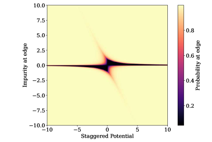
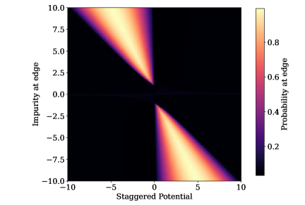
Figure 21: Probabilities $|\psi(0)|^{2}$ of the states with the largest two IPR values at the left edge of a 100-site system versus $(v,A)$. The probability is larger in the lighter colored regions. Plot (a) shows that one edge state exists for a large range of parameters values, while plot (b) shows that a second edge state exists in some smaller regions of parameters. We have set $g=1$.

We will now evaluate the right-hand side of Eq. (52) by using the resolution of identity written in terms of the basis of eigenstates of $H_{0}$. Since $H_{0}$ has a staggered potential, its unit cell has two sites which we will call $(a,b)$. The sites which were earlier labeled as $n=0,1,2,\cdots$ will now denote $(a,n/2)$ if $n$ is even and $(b,(n-1)/2)$ if $n$ is odd. We can then write

$$H_{0} = \sum_{m=0}^{\infty}~{}[(a_{m}^{\dagger}b_{m}~{}+~{}b_{m}^{\dagger}a_{m}~{}+~{}b_{m}^{\dagger}a_{m+1}~{}+~{}a_{m+1}^{\dagger}b_{m})$$ (53)

$$~{}~{}~{}~{}~{}~{}~{}~{}~{}+~{}v~{}(a_{m}^{\dagger}a_{m}~{}-~{}b_{m}^{\dagger}b_{m})].$$

We can find the eigenvalues and eigenstates of this Hamiltonian as follows. If the sum over $m$ went from $-\infty$ to $\infty$, we could use translation invariance and find that the energy eigenvalues are given by

$$E_{k,\pm}~{}=~{}\pm~{}\sqrt{4g^{2}\cos^{2}k~{}+~{}v^{2}},$$ (54)

where $\pm$ denote the positive and negative energy bands respectively, the eigenstates have the plane wave form

$$\psi(a,m,k,\pm) = \alpha_{k,\pm}~{}e^{ikm},$$

$$\psi(b,m,k,\pm) = \beta_{k,\pm}~{}e^{ikm},$$ (55)

where

$$\alpha_{k,\pm} = -~{}\frac{2g\cos k}{\sqrt{(E_{k,\pm}~{}-~{}v)^{2}~{}+~{}4g^{2}\cos^{2}k}},$$

$$\beta_{k,\pm} = \frac{E_{k,\pm}~{}-~{}v}{\sqrt{(E_{k,\pm}~{}-~{}v)^{2}~{}+~{}4g^{2}\cos^{2}k}},$$ (56)

and the momentum $k$ lies in the range $[-\pi/2,\pi/2]$ since the unit cell spacing is equal to 2 in terms of the original lattice spacing. Now, since our system ends on the left at the site $(a,0)$, we can find its eigenstates by appropriately superposing the momentum eigenstates corresponding to $\pm k$ in such a way that the wave function vanishes at the ‘phantom’ sites given by $(a,m=-1)$ and $(b,m=-1)$. Noting that the expressions in Eqs. (56) are even functions of $k$, we then find that the eigenstates of the semi-infinite chain are given by

$$\psi(a,m,k,\pm) = \sqrt{2}~{}\alpha_{k,\pm}~{}\sin(k(m+1)),$$

$$\psi(b,m,k,\pm) = \sqrt{2}~{}\beta_{k,\pm}~{}\sin(k(m+1)),$$ (57)

where the $\sqrt{2}$ has been put in to ensure orthonormality, and $k$ now lies in the range $[0,\pi/2]$. The wave function for the state $|k,\pm\rangle$ at the leftmost site, $(a,m=0)$, is therefore given by $\sqrt{2}\alpha_{k,\pm}\sin k$.

We can now use the above eigenstates $|k,\pm\rangle$ to write the resolution of identity:

$$\int_{0}^{\pi/2}\frac{dk}{\pi/2}~{}(|k,+\rangle\langle k,+|~{}+~{}|k,-\rangle\langle k,-|)~{}=~{}I.$$ (58)

Using this in Eq. (52), we obtain

$$\frac{1}{A} = \int_{0}^{\pi/2}\frac{dk}{\pi/2}~{}[\langle 0|\frac{1}{E~{}I~{}-~{}H_{0}}|k,+\rangle\langle k,+|0\rangle$$

$$~{}~{}~{}~{}~{}~{}~{}~{}~{}~{}~{}~{}~{}~{}~{}~{}~{}~{}~{}+~{}\langle 0|\frac{1}{E~{}I~{}-~{}H_{0}}|k,-\rangle\langle k,-|0\rangle]$$

$$= \int_{0}^{\pi/2}\frac{dk}{\pi/2}~{}2\sin^{2}k~{}\left[\frac{|\alpha_{k,+}|^{2}}{E~{}-~{}E_{k,+}}~{}+~{}\frac{|\alpha_{k,-}|^{2}}{E~{}-~{}E_{k,-}}\right].$$

(The above equation is only valid for $E$ lying outside the energy bands $E_{k,\pm}$, otherwise the denominators can vanish and we would have to evaluate the integral more carefully). Substituting the expression for $\alpha_{k,\pm}$ in Eq. (56) in Eq. (LABEL:ls12), we obtain

$$\frac{1}{A} = \int_{0}^{\pi/2}\frac{dk}{\pi}~{}16g^{2}\sin^{2}k\cos^{2}k$$

$$\times~{}[\frac{1}{(E-E_{k,+})~{}[(E_{k,+}-v)^{2}~{}+~{}4g^{2}\cos^{2}k]}$$

$$~{}~{}~{}+~{}\frac{1}{(E-E_{k,-})~{}[(E_{k,-}-v)^{2}~{}+~{}4g^{2}\cos^{2}k]}].$$

Now, if an edge state exists, its energy $E$ must lie either above the upper band ($E>\sqrt{4g^{2}+v^{2}}$), or below the lower band ($E<-\sqrt{4g^{2}+v^{2}}$), or in the gap between the two bands ($-v<E<v$). In the first two cases, the integral in Eq. (LABEL:ls13) gives the result

$$A~{}=~{}\dfrac{E^{2}~{}-~{}v^{2}~{}+~{}\sqrt{(E^{2}~{}-~{}v^{2})(E^{2}~{}-~{}4g^{2}~{}-~{}v^{2})}}{2(E~{}+~{}v)}.$$ (61)

In the third case, Eq. (LABEL:ls13) gives

$$A~{}=~{}-~{}\dfrac{v^{2}~{}-~{}E^{2}~{}+~{}\sqrt{(v^{2}~{}-~{}E^{2})(4g^{2}~{}+~{}v^{2}-E^{2})}}{2(v~{}+~{}E)}.$$ (62)

Equations (61) and (62) implicitly give the energy $E$ of an edge state in terms of $g$, $v$, and $A$. We find that these give certain conditions on the allowed values of $A$ for a given value of $(g,v)$.

(i) $E<-\sqrt{4g^{2}+v^{2}}$ implies that we must have $A<A_{1}$, where

$$A_{1}~{}=~{}\frac{2g^{2}}{v~{}-~{}\sqrt{v^{2}~{}+~{}4g^{2}}}.$$ (63)

(ii) $E>\sqrt{4g^{2}+v^{2}}$ implies that $A>A_{2}$, where

$$A_{2}~{}=~{}\frac{2g^{2}}{v~{}+~{}\sqrt{v^{2}~{}+~{}4g^{2}}}.$$ (64)

(iii) $-v<E<v$ implies that if $v>0$, we must have $A<0$, while if $v<0$, we must have $A>0$. Namely, we must have

$$Av~{}<~{}0.$$ (65)

The regions described by Eqs. (63-65) are shown in Fig. 22. We see that these agree well with the regions of bound states (light regions) shown in Figs. 21 (a) and (b). In particular, they correctly tell us that there are two bound states in the regions shown in Fig. 21 (b).

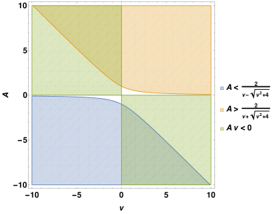
Figure 22: Three colors showing regions of $A$ as a function of $v$ where edge states exist. The regions where two colors overlap have two edge states. We have taken $g=1$.

As a special case of the above results, it is interesting to consider what happens if we set $v=0$; this will also be useful for the next section. Namely, we only have a potential $A$ at the site $n=0$. Equations (63-64) then imply that there will be a bound state if either $A<-g$ or $A>g$. The bound state energy and wave function can be derived easily. For $A<-g$, we find that the wave function and energy are given by

$$\psi(n) = e^{-\kappa n},~{}~{}~{}{\rm where}~{}~{}~{}n~{}\geq~{}0,$$

$$E = -2g\cosh\kappa,~{}~{}~{}{\rm and}~{}~{}~{}e^{\kappa}~{}=~{}-~{}\frac{A}{g},$$ (66)

where $\kappa>0$. For $A>g$, we have

$$\psi(n) = (-1)^{n}~{}e^{-\kappa n},$$

$$E = 2g\cosh\kappa,~{}~{}~{}{\rm and}~{}~{}~{}e^{\kappa}~{}=~{}\frac{A}{g}.$$ (67)

For $v=0$, we have seen above that the condition $|A|>|g|$ is required in order to have an edge state. We can now understand why there are no edge states in the periodically driven system if $\omega$ is very large. Equation (LABEL:heff2) shows that the effective hopping is $-gJ_{0}(a/\omega)$, and the effective edge potential is given by $-(4g^{2}/\omega)J_{0}(a/\omega)\sum_{p=1,3,5,\cdots}J_{p}(a/\omega)/p$. Clearly, when $\omega$ becomes sufficiently large, the effective edge potential will become smaller in magnitude than the effective hopping, and there will not be any edge states.

C.2 Bose-Hubbard model

For the Bose-Hubbard model with an edge potential as described in Eq. (47), we consider a 25-site system with two bosons and numerically find the probability of the two particles to be at the edge, $|\psi(0,0)|^{2}$, as a function of the parameters $(u,A)$. The results are shown in Figs. 23 (a) and (b) for the states with the largest two IPR values. Just as in Fig. 21, there can be zero, one or two two-particle bound states which are localized near the leftmost site of the system.

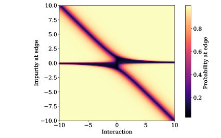
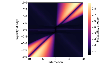
Figure 23: Probabilities $|\psi(0,0)|^{2}$ of the two highest IPR states at the left edge of a 25-site system plotted versus $(u,A)$. The probability is higher in the lighter colored regions. Plot (a) shows that one edge state exists for a large range of parameter values, while plot (b) shows that a second edge state exists in some smaller regions of parameters. We have set $g=1$.

We can understand the existence of a two-particle bound state localized near $n=0$ using a perturbative argument in the limit $|u|\gg|g|,|A|$. To see this, we write the Hamiltonian in Eq. (47) in the form $H=H_{0}+V$, where

$$H_{0} = \frac{u}{2}~{}\sum_{n=0}^{\infty}\rho_{n}(\rho_{n}-1)~{}+~{}A~{}b_{0}^{\dagger}b_{0},$$

$$V = -~{}g~{}\sum_{n=0}^{\infty}~{}(b_{n}^{\dagger}b_{n+1}~{}+~{}b_{n+1}^{\dagger}b_{n}).$$ (68)

We now consider a system with two particles. The eigenstates of $H_{0}$ are of the following kinds. States where there is no particle at $n=0$ and no site has more than one particle (all these states have zero energy), there is one particle at $n=0$ and the other particle is at some other site (these states have energy $A$), the two particles are at the same site which is not at $n=0$ (these have energy $u$), and both the particles are at $n=0$ (this state has energy $u+2A$). We will now work within the space of states where the two particles are at the same site (which may or may not by $n=0$) and derive an effective Hamiltonian within this space to second order in $g$ (i.e., the perturbation $V$ in Eq. (68)).

Starting with an initial state $|n,n\rangle$ (where $n=0,1,2,\cdots$), the hopping can take us to a final state $|n+1,n+1\rangle$ (or $|n-1,n-1\rangle$) through the intermediate state $|n,n+1\rangle$ (or $|n-1,n\rangle$ respectively). The matrix element connecting the initial or final state to the intermediate state is $-g\sqrt{2}$. The energy denominator, given by the difference of the initial and intermediate state energies, is given by $u$ (if $n=0$, the energy denominator is $u+2A$, but we can approximate this by $u$ since we are assuming that $|u|\gg|A|$). The hopping can also take us from a state $|n,n\rangle$ back to the same state $|n,n\rangle$ in two ways (through the intermediate states ($|n,n+1\rangle$ and $|n-1,n\rangle$) if $n\geq 1$ but in only one way (through the intermediate state $|0,1\rangle$) if $n=0$. Putting all this together and using the notation $|n\rangle$ to denote the state in which both particles are at site $n$ and $d_{n}$ and $d_{n}^{\dagger}$ as the annihilation and creation operator for two particles at site $n$, we see that the effective Hamiltonian in this space is given by

$$H_{eff} = ~{}\frac{2g^{2}}{u}~{}\sum_{n=0}^{\infty}~{}(d_{n}^{\dagger}d_{n+1}~{}+~{}d_{n+1}^{\dagger}d_{n})$$

$$+(u+2A+\frac{2g^{2}}{u})~{}d_{0}^{\dagger}d_{0}+(u+\frac{4g^{2}}{u})~{}\sum_{n=1}^{\infty}~{}d_{n}^{\dagger}d_{n}.$$

We see that this Hamiltonian has a single particle (which is actually a pair of bosons) hopping amplitude given by $2g^{2}/u$, a chemical potential $u+4g^{2}/u$ at all sites, and a potential $2A-2g^{2}/u$ at the site $n=0$. We now see that if $u>0$, the result for a single particle with an edge potential discussed at the end of the previous section implies that there will be a bound state localized near $n=0$ if either $2A-2g^{2}/u<-2g^{2}/u$ or $2A-2g^{2}/u>2g^{2}/u$, i.e., if

$${\rm either}~{}~{}~{}A~{}<~{}0~{}~{}~{}{\rm or}~{}~{}~{}A~{}>~{}\frac{2g^{2}}{u}.$$ (70)

If $u<0$, these conditions change to $2A-2g^{2}/u<2g^{2}/u$ or $2A-2g^{2}/u>-2g^{2}/u$, i.e.,

$${\rm either}~{}~{}~{}A~{}<~{}\frac{2g^{2}}{u}~{}~{}~{}{\rm or}~{}~{}~{}A~{}>~{}0.$$ (71)

We see that Eqs. (70) and (71)) correctly describe the regions of bound states in Fig. 23 (a) for $u>0$ and $u<0$ respectively, when $|A|\ll|u|$.

When $|u|,|A|\gg|g|$, but $|u|$ and $|A|$ are of the same order, the perturbation theory described above breaks down. However, we can understand why there are no two-particle bound states localized near $n=0$ close to the line $u+A=0$ as we see in Fig. 23 (a). Ignoring the hopping $g$ entirely, we know that the state where both particles are at $n=0$ has energy $u+2A$ while all the states where one particle is at $n=0$ and the other particle is at any other state have energy $A$. If these two states have the same energy, and a small hopping $g$ is turned on, the state with two particles at $n=0$ will mix with the states where one particle remains at $n=0$ and the other particle escapes far away from there. Hence we no longer have a two-particle bound state localized near $n=0$ as an eigenstate of the Hamiltonian.

The above arguments do not explain the existence of a second bound state that we see in Fig. 23 (b) in some small regions in the parameter space.

References

- (1)
- (2) F. Grossmann, T. Dittrich, P. Jung, and P. Hänggi, Phys. Rev. Lett. 67, 516 (1991).
- (3) Y. Kayanuma, Phys. Rev. A 50, 843 (1994).
- (4) A. Das, Phys. Rev. B 82, 172402 (2010).
- (5) A. Russomanno, A. Silva, and G. E. Santoro, Phys. Rev. Lett. 109, 257201 (2012).
- (6) T. Nag, S. Roy, A. Dutta, and D. Sen, Phys. Rev. B 89, 165425 (2014).
- (7) S. Sharma, A. Russomanno, G. E. Santoro, and A. Dutta, EPL 106, 67003 (2014); A. Russomanno, S. Sharma, A. Dutta and G. E. Santoro, J. Stat. Mech. (2015) P08030.
- (8) A. Lazarides, A. Das, and R. Moessner, Phys. Rev. Lett. 112, 150401 (2014).
- (9) A. Dutta, G. Aeppli, B. K. Chakrabarti, U. Divakaran, T. Rosenbaum, and D. Sen, Quantum Phase Transitions in Transverse Field Spin Models: From Statistical Physics to Quantum Information (Cambridge University Press, Cambridge, 2015).
- (10) A. Lubatsch and R. Frank, Symmetry 11, 1246 (2019), and Eur. Phys. J. B 92, 215 (2019).
- (11) I. Bloch, Nature Phys. 1, 23 (2005).
- (12) T. Kitagawa, M. A. Broome, A. Fedrizzi, M. S. Rudner, E. Berg, I. Kassal, A. Aspuru-Guzik, E. Demler, and A. G. White, Nature Commun. 3, 882 (2012).
- (13) L. Tarruell, D. Greif, T. Uehlinger, G. Jotzu, and T. Esslinger, Nature (London) 483, 302 (2012).
- (14) M. C. Rechtsman, J. M. Zeuner, Y. Plotnik, Y. Lumer, D. Podolsky, S. Nolte, F. Dreisow, M. Segev, and A. Szameit, Nature (London) 496, 196 (2013); M. C. Rechtsman, Y. Plotnik, J. M. Zeuner, D. Song, Z. Chen, A. Szameit, and M. Segev, Phys. Rev. Lett. 111, 103901 (2013); Y. Plotnik, M. C. Rechtsman, D. Song, M. Heinrich, J. M. Zeuner, S. Nolte, Y. Lumer, N. Malkova, J. Xu, A. Szameit, Z. Chen, and M. Segev, Nature Mater. 13, 57 (2014).
- (15) T. Langen, R. Geiger, and J. Schmiedmayer, Annu. Rev. Condens. Matter Phys. 6, 201 (2015).
- (16) G. Jotzu, M. Messer, R. Desbuquois, M. Lebrat, T. Uehlinger, D. Greif, and T. Esslinger, Nature (London) 515, 237 (2014).
- (17) A. Eckardt, Rev. Mod. Phys. 89, 011004 (2017).
- (18) S. A. Sato, J. W. McIver, M. Nuske, P. Tang, G. Jotzu, B. Schulte, H. Hübener, U. De Giovannini, L. Mathey, M. A. Sentef, A. Cavalleri, and A. Rubio, Phys. Rev. B 99, 214302 (2019); J. W. McIver, B. Schulte, F.-U. Stein, T. Matsuyama1, G. Jotzu, G. Meier, and A. Cavalleri, Nature Phys. 16, 38 (2020).
- (19) D. H. Dunlap and V. M. Kenkre, Phys. Rev. B 34, 3625 (1986).
- (20) A. Agarwala, U. Bhattacharya, A. Dutta and D. Sen, Phys. Rev. B 93, 174301 (2016).
- (21) A. Agarwala and D. Sen, Phys. Rev. B 95, 014305 (2017).
- (22) T. Oka and H. Aoki, Phys. Rev. B 79, 081406(R) (2009); T. Kitagawa, T. Oka, A. Brataas, L. Fu, and E. Demler, Phys. Rev. B 84, 235108 (2011).
- (23) T. Kitagawa, E. Berg, M. Rudner, and E. Demler, Phys. Rev. B 82, 235114 (2010).
- (24) N. H. Lindner, G. Refael, and V. Galitski, Nature Phys. 7, 490 (2011).
- (25) L. Jiang, T. Kitagawa, J. Alicea, A. R. Akhmerov, D. Pekker, G. Refael, J. I. Cirac, E. Demler, M. D. Lukin, and P. Zoller, Phys. Rev. Lett. 106, 220402 (2011).
- (26) Z. Gu, H. A. Fertig, D. P. Arovas, and A. Auerbach, Phys. Rev. Lett. 107, 216601 (2011).
- (27) M. Trif and Y. Tserkovnyak, Phys. Rev. Lett. 109, 257002 (2012).
- (28) A. Gomez-Leon and G. Platero, Phys. Rev. B 86, 115318 (2012), and Phys. Rev. Lett. 110, 200403 (2013).
- (29) B. Dóra, J. Cayssol, F. Simon, and R. Moessner, Phys. Rev. Lett. 108, 056602 (2012).
- (30) J. Cayssol, B. Dora, F. Simon, and R. Moessner, Phys. Status Solidi RRL 7, 101 (2013).
- (31) D. E. Liu, A. Levchenko, and H. U. Baranger, Phys. Rev. Lett. 111, 047002 (2013).
- (32) Q.-J. Tong, J.-H. An, J. Gong, H.-G. Luo, and C. H. Oh, Phys. Rev. B 87, 201109(R) (2013).
- (33) M. S. Rudner, N. H. Lindner, E. Berg, and M. Levin, Phys. Rev. X 3, 031005 (2013); F. Nathan and M. S. Rudner, New J. Phys. 17, 125014 (2015).
- (34) Y. T. Katan and D. Podolsky, Phys. Rev. Lett. 110, 016802 (2013).
- (35) N. H. Lindner, D. L. Bergman, G. Refael, and V. Galitski, Phys. Rev. B 87, 235131 (2013).
- (36) A. Kundu and B. Seradjeh, Phys. Rev. Lett. 111, 136402 (2013).
- (37) A. Kundu, H. A. Fertig, and B. Seradjeh, Phys. Rev. Lett. 113, 236803 (2014).
- (38) T. L. Schmidt, A. Nunnenkamp, and C. Bruder, New J. Phys. 15, 025043 (2013).
- (39) A. A. Reynoso and D. Frustaglia, Phys. Rev. B 87, 115420 (2013).
- (40) C.-C. Wu, J. Sun, F.-J. Huang, Y.-D. Li, and W.-M. Liu, EPL 104, 27004 (2013).
- (41) M. Thakurathi, A. A. Patel, D. Sen, and A. Dutta, Phys. Rev. B 88, 155133 (2013); M. Thakurathi, K. Sengupta, and D. Sen, Phys. Rev. B 89, 235434 (2014).
- (42) P. M. Perez-Piskunow, G. Usaj, C. A. Balseiro, and L. E. F. Foa Torres, Phys. Rev. B 89, 121401(R) (2014); G. Usaj, P. M. Perez-Piskunow, L. E. F. Foa Torres, and C. A. Balseiro, Phys. Rev. B 90, 115423 (2014); P. M. Perez-Piskunow, L. E. F. Foa Torres, and G. Usaj, Phys. Rev. A 91, 043625 (2015).
- (43) M. D. Reichl and E. J. Mueller, Phys. Rev. A 89, 063628 (2014).
- (44) D. Carpentier, P. Delplace, M. Fruchart, and K. Gawedzki, Phys. Rev. Lett. 114, 106806 (2015).
- (45) T.-S. Xiong, J. Gong, and J.-H. An, Phys. Rev. B 93, 184306 (2016).
- (46) M. Thakurathi, D. Loss, and J. Klinovaja, Phys. Rev. B 95, 155407 (2017).
- (47) L. Zhou and J. Gong, Phys. Rev. B 97, 245430 (2018).
- (48) O. Deb and D. Sen, Phys. Rev. B 95, 144311 (2017).
- (49) S. Saha, S. N. Sivarajan and D. Sen, Phys. Rev. B 95, 174306 (2017).
- (50) S. Longhi and G. D. Valle, Sci. Rep. 3, 2219 (2013).
- (51) C. González-Santander, P. A. Orellana, and F. Domínguez-Adame, Europhys. Lett. 102, 17012 (2013).
- (52) B. Zhu, Y. Ke, W. Liu, Z. Zhou, and H. Zhong, Phys. Rev. A 102, 023303 (2020).
- (53) R. L. Schult, D. G. Ravenhall, and H. W. Wyld, Phys. Rev. B 39, 5476(R) (1989).
- (54) R. A. Pinto, M. Haque, and S. Flach, Phys. Rev. A 79, 052118 (2009).
- (55) R. Peierls, Zeitschrift für Physik 80, 763 (1933).
- (56) M. Bukov, L. D’Alessio, and A. Polkovnikov, Advances in Physics 64, 139 (2015).
- (57) T. Mikami, S. Kitamura, K. Yasuda, N. Tsuji, T. Oka, and H. Aoki, Phys. Rev. B 93, 144307 (2016).
- (58) A. Soori and D. Sen, Phys. Rev. B 82, 115432 (2010).
- (59) B. Mukherjee, S. Nandy, A. Sen, D. Sen, and K. Sengupta, Phys. Rev. B 101, 245107 (2020).
- (60) A. Haldar, D. Sen, R. Moessner and A. Das, arXiv:1909.04064.
- (61) M. Moskalets and M. Büttiker, Phys. Rev. B 66, 205320 (2002).
- (62) A. Agarwal and D. Sen, Phys. Rev. B 76, 235316 (2007).
- (63) H. Lignier, C. Sias, D. Ciampini, Y. Singh, A. Zenesini, O. Morsch, and E. Arimondo, Phys. Rev. Lett. 99, 220403 (2007).
- (64) C. Chin, R. Grimm, P. Julienne, and E. Tiesinga, Rev. Mod. Phys. 82, 1225 (2010).
- (65) S. Trotzky, L. Pollet, F. Gerbier, U. Schnorrberger, I. Bloch, N. Prokof’ev, B. Svistunov, and M. Troyer, Nature Phys. 6, 998 (2010).
- (66) J. H. Shirley, Phys. Rev. 138, B 979 (1965).
- (67) M. Abramowitz and I. A. Stegun, Handbook of Mathematical Functions (Dover, New York, 1972).