Cold-start Sequential Recommendation via Meta Learner

Abstract

This paper explores meta-learning in sequential recommendation to alleviate the item cold-start problem. Sequential recommendation aims to capture user’s dynamic preferences based on historical behavior sequences and acts as a key component of most online recommendation scenarios. However, most previous methods have trouble recommending cold-start items, which are prevalent in those scenarios. As there is generally no side information in the setting of sequential recommendation task, previous cold-start methods could not be applied when only user-item interactions are available. Thus, we propose a Meta-learning-based Cold-Start Sequential Recommendation Framework, namely Mecos, to mitigate the item cold-start problem in sequential recommendation. This task is non-trivial as it targets at an important problem in a novel and challenging context. Mecos effectively extracts user preference from limited interactions and learns to match the target cold-start item with the potential user. Besides, our framework can be painlessly integrated with neural network-based models. Extensive experiments conducted on three real-world datasets verify the superiority of Mecos, with the average improvement up to 99%, 91%, and 70% in HR@10 over state-of-the-art baseline methods.

Introduction

Increasing research interests have been attracted in sequential recommendation due to its highly practical value in online services (e.g., e-commerce), where users’ current interest are intrinsically dynamic as the evolving of their historical actions. Accurately recommending the user’s next action based only on the sequential dynamic of historical interactions lies in the heart of sequential recommendation.

Markov Chains (MC) (Zimdars, Chickering, and Meek 2001) is a representation of traditional methods, which predicts the user’s next action based on the previous one. Recently, neural network-based methods have become popular due to their strong abilities to model sequential data, such as the methods based on recurrent neural network (RNN) (Hidasi et al. 2015; Tan, Xu, and Liu 2016; Li et al. 2017; Cui et al. 2018), Attention (Liu et al. 2018; Kang and McAuley 2018), convolutional neural network (CNN) (Tang and Wang 2018), and graph neural network (GNN) (Wu et al. 2019; Zheng et al. 2020). For example, NARM (Li et al. 2017) employs RNNs with an attention mechanism to capture the main purpose and sequential behavior, then combines them as a representation for the recommendation. SR-GNN (Wu et al. 2019) models the session data in the graph structure and utilizes a gated GNN to model complex transitions among item nodes.

These sequential recommendation models mainly rely on user-item interactions to portray user preference and item property. Therefore, the number of historical interactions largely determines the model performance. However, new items arrive frequently in those online services, and timely recommending these items to the target users is of high practical value. As they rarely have enough known interactions with users, existing models have trouble in recommendation towards those items. Therefore, cold-start problem needs to be solved in sequential recommendation scenarios.

The basic idea behind existing cold-start methods in the general recommendation is to incorporate side information, such as user and item attributes (e.g., user profile, item ratings or descriptions) (Barjasteh et al. 2016; Saveski and Mantrach 2014) and knowledge from other domains (Hu, Zhang, and Yang 2018). Recently, some meta-learning approaches have been proposed to tackle it (Vartak et al. 2017; Yao et al. 2019; Lee et al. 2019; Du et al. 2019; Dong et al. 2020), but they still cannot get rid of these side information. For example, $s^{2}$Meta (Du et al. 2019) relies on cross-domain knowledge transferring. Vartak et al. (Vartak et al. 2017) utilize item ratings to make the twitter recommendation. MAMO (Dong et al. 2020) predicts the rating for new items with the help of user profile and item descriptions. However, because there is generally no side information in the setting of sequential recommendation task, previous cold-start methods, including those based on meta-learning, cannot be applied in these scenarios. Therefore, the cold-start problem in sequential recommendation remains unexplored.

To alleviate the item cold-start problem in sequential scenarios given only sparse interactions, we propose a MEta-learning-based COld-start Sequential recommendation framework (Mecos). Our framework can be painlessly integrated with neural network-based sequential recommendation models. We first design a sequence pair encoder to effectively extract user preference. Then a matching network is applied to match the query sequence pair to the support set corresponding to the candidate cold-start item. Moreover, we employ the meta-learning based gradient descent approach for parameter optimization. Once trained, the learned metric model can be applied to make recommendations for new items without further fine-tuning. Extensive experiments show the superiority of Mecos in dealing with cold-start items in sequential recommendation.

The main contribution of this work is threefold. First, we propose Mecos framework for sequential scenarios to alleviate the item cold-start problem. To the best of our knowledge, this is the first work to tackle this problem. The task is non-trivial as it aims at a classical problem in a novel and challenging context, where the only available data is the user-item interaction. Second, our framework can be easily integrated with existing neural network-based sequential recommendation models. And once trained, Mecos can be adapted to new items without further fine-tuning. Lastly, we compare Mecos with state-of-the-art methods on three public datasets. Results demonstrate the effectiveness of our framework. And a comprehensive ablation study is conducted to analyze the contributions of the key components.

Related Work

Sequential Recommendation

Neural networks-based recommenders (Wu et al. 2020; Li et al. 2020) have attracted much attention due to their effect in modeling sequential data. RNN with a gated recurrent unit (Hidasi et al. 2015) achieves significant improvement compared with conventional methods. To further improve it, an encoder-decoder model (NARM) applying attention mechanism (Li et al. 2017) is proposed to extract more representative features. Besides these RNN-based methods, CNN is used in Caser (Tang and Wang 2018) to learn local features of a sequence ”image” using convolutional filters. Moreover, to explicitly model the impact of items of different time steps on the current decision, attention-based models are also developed in sequential recommendation, such as STAMP and SASRec (Liu et al. 2018; Kang and McAuley 2018; Liu and Zheng 2020). As GNN becomes popular, it is also employed to model sequential data into graph-structured data to capture complex items transitions (Wu et al. 2019; Yu et al. 2020). Recent works (Zheng, Liu, and Zhou 2019; Zheng et al. 2020) introduced cross-session item transitions. Different from these methods, we explore few-shot learning to alleviate the item cold-start problem in sequential recommendation.

Cold-start Recommendation

The common solution to address cold-start recommendation is to utilize side information, such as auxiliary and contextual information (Barjasteh et al. 2016; Saveski and Mantrach 2014) and knowledge from other domains (Hu, Zhang, and Yang 2018). Traditional content-based methods augment the data with user or item features. Saveski and Mantrach (Saveski and Mantrach 2014) proposed a local collective embedding learning method to exploits items’ properties and user preferences. DecRec (Barjasteh et al. 2016) decouples the rating sub-matrix completion and knowledge transduction from ratings to exploit the side information. Besides, based on the assumption that the same user or item can be located in different scenarios, transferring-based methods (Hu, Zhang, and Yang 2018; Kang et al. 2019) use cross-domain knowledge to mitigate cold-start problems in a new scenario.

Meta-learning in Cold-start Recommendation

Recently, meta-learning for recommender systems has been attracting attention. Most of these works focus on the recommendation scenarios with few training samples because it is natural to turn these tasks into few-shot learning problems. For example, Vartak et al. (Vartak et al. 2017) propose two network architectures based on a meta-learning strategy to predict the user’s rating for twitters based on historical item ratings. $s^{2}$Meta (Du et al. 2019) initializes the recommender with a sequential learning process based on cross-domain knowledge transferring. Li et al. (Li et al. 2019) formulate cold-start recommendation as a zero-shot learning task with user profiles. MeLU (Lee et al. 2019) integrates both user and item attributes and identifies reliable evidence candidates for customized preference estimation. Also relying on user and item side information, MAMO (Dong et al. 2020) uses two designed memory matrices to avoid the local optima for users with a specific pattern. However, as they all rely on side information (e.g., user profile, item attributes, and cross-domain knowledge) to leverage limited training data, they cannot be applied in the sequential recommendation, where the only data that is always available is the user-item interaction. Different from them, our work introduces a general framework to alleviate cold-start problem based only on user-item interactions.

Preliminary

Problem Formulation

In sequential recommendation, a dataset can be represented as a collection of user-item sequences. Let $\mathcal{U}$ and $\mathcal{V}$ represent the user set and item set respectively. And $\zeta_{i}=(v_{i,1},v_{i,2},...,v_{i,n})$ denotes the interaction sequence generated by user $u_{i}\in\mathcal{U}$ in the chronological order. The aim of sequential recommendation model is to recommend the next item $v_{i,n+1}$ that the user $u_{i}$ will interact with based on $\zeta_{i}$. Thus, it is equal to predict next item $v_{i,n+1}$ based on the query sequence pair $(\zeta_{i},\text{?})$. To achieve that, the model will generate a score for each candidate item in the item set $\mathcal{V}$. Then items with a top-$p$ recommendation score will be recommended as the model’s output.

In our task, we have a set of cold-start items $\mathcal{Y}\subset\mathcal{V}$, that every single item in $\mathcal{Y}$ only has a few interactions with users in the dataset. Different from other sequential recommendation models that rely on rich training instances, our goal is to recommend cold-start items with few-shot examples. We use $\mathcal{Y}_{\text{train}}$ and $\mathcal{Y}_{\text{test}}$ to represent the training and testing instances, where $\mathcal{Y}_{\text{test}}\cap\mathcal{Y}_{\text{train}}=\phi$.

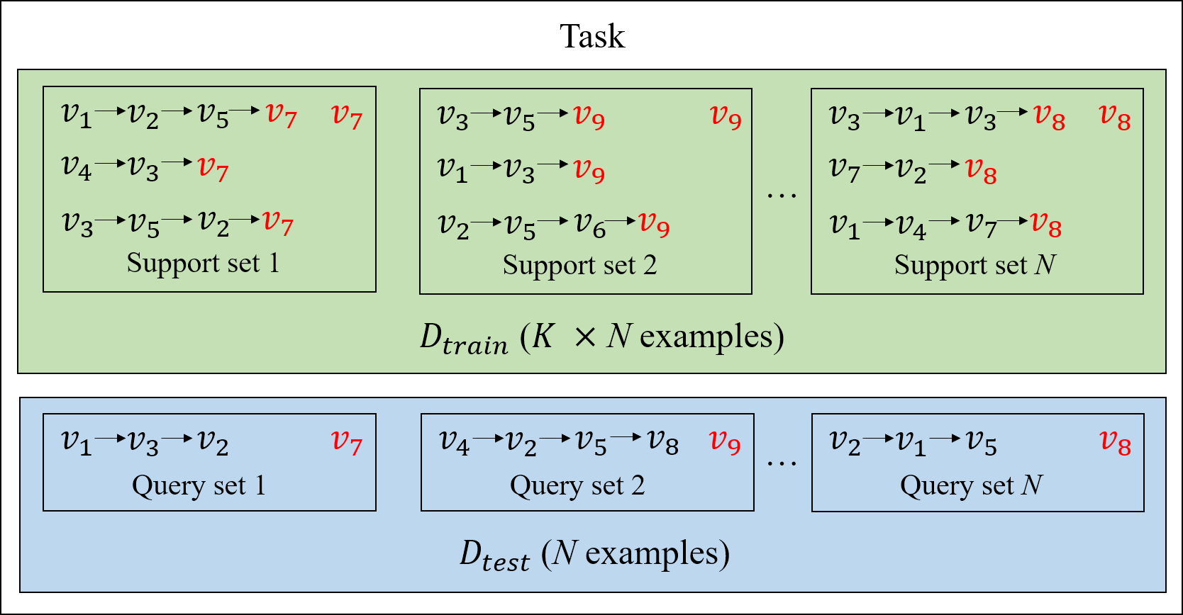
Figure 1: Single task with $K=3$ and $N$ different support sets. Each query set is the query sequence pair that needs to be matched with a candidate cold-start item (red) corresponding to the support set. When $K=3$, we have three training instances for our target item. And $N$ is the size of candidate cold-start items set.

Meta-training

Following the standard meta-learning settings, we train our model based on a set of training tasks $\mathcal{T}_{\text{meta-train}}$. To create a training task $T_{i}\in\mathcal{T}_{\text{meta-train}}$ (Figure 1), we first sample $N$ next-click items from $\mathcal{Y}_{\text{train}}$. For each of those $N$ items, we sample $K$ sequence pairs, where each pair $(\zeta_{i},v_{i,n+1})$ represents a sequence $\zeta_{i}$ and its ground-truth next-click item $v_{i,n+1}$, as the support set. As the cold-start item is recommended to one user at each time, the query set is represented by a single query sequence pair $(\zeta_{i},\text{?})$. We denote those $N$ support/query sets in task $T_{i}$ as $D_{i}^{\text{train}}$ and $D_{i}^{\text{test}}$, respectively. Then the query set will match over all support sets to calculate the similarities between them. The similarity score will be handled as the recommendation score of the candidate next-click item in the corresponding support set. Since we employed the data augmentation on the datasets as previous methods (Liu et al. 2018; Wu et al. 2019) (e.g., a sequence $(v_{0},v_{1},v_{2},v_{3})$ is divided into three successive sequences: $(v_{0},v_{1})$, $(v_{0},v_{1},v_{2})$, $(v_{0},v_{1},v_{2},v_{3})$), the candidate next-click items are actually distributed in all positions of the original sequence thus they are equal to the candidate items. Then the loss can be calculated by the ground-truth next-click item and the recommended one. We will elaborate these in the next sections.

Meta-testing

After training, the model can make predictions for the task with $N$ new ground-truth items from $\mathcal{Y}_{\text{test}}$, which is the meta-testing step. These meta-testing ground-truth items are unseen from the meta-training. The same as meta-training, each meta-testing task also has its few-shot training data and testing data. And these tasks form the meta-test set $\mathcal{T}_{\text{meta-test}}$. Moreover, we randomly leave out a subset of labels in $\mathcal{Y}_{\text{train}}$ to generate the validation set $\mathcal{T}_{\text{meta-valid}}$.

Now we can define our total meta-learning task set as $\mathcal{T}=\mathcal{T}_{\text{meta-train}}\bigcup\mathcal{T}_{\text{meta-test}}\bigcup\mathcal{T}_{\text{meta-valid}}$.

Integrating with Existing Methods

With the input of pre-trained item embeddings generated by existing sequential recommendation models, Mecos can be easily integrated with these methods to improve their performance in cold-start scenarios. Based on our setting, tasks that their ground-truth next-click items have rich interactions will be excluded from $\mathcal{T}$. And these data will be selected for the training of pre-trained item embeddings. To ensure those ground-truth items will not be seen before meta-learning tasks, sequences in pre-trained datasets will be removed when they contain the ground-truth item in $\mathcal{T}$.

It is noteworthy that we are not introducing more complexity or training with more data based on the baseline models. The purpose of pre-training is to make sure that both models with or without Mecos have a similar quality of embeddings for items with rich interactions. And all models are training with the same amount of data. Under these circumstances, we can make a fair comparison of recommendation performance toward cold-start items.

Mecos

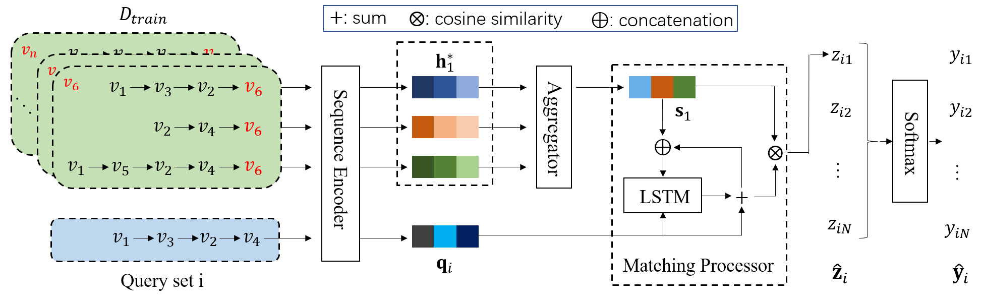
Figure 2: The framework of Mecos. The green square represents a support set that contains few-shot training sequences of a candidate cold-start item (red). Our goal is to recommend cold-start items to the query sequence (blue square). It first generates sequence pair representations (Eq. 1, 2), then aggregates few-shot sequence representations to generate support set representation (Eq. 3). Finally, it employs a matching network (Eq. 4) to compute similarity scores between the query set and all support sets (Eq. 5). After matching the $i$-th query set with $N$ different support sets, we can get a vector of similarity scores $\hat{\mathbf{z}}_{i}$. Then a softmax function is applied to generate the $i$-th query set’s final recommendation score of each candidate item, denoted as $\hat{\mathbf{y}}_{i}$.

In this section, we elaborate on the details of Mecos (Figure 2). With the pre-trained item embeddings as inputs, Mecos first encodes sequence pairs into representation vectors, then aggregates them to generate the support/query set representations. After that, a matching network is employed to match the query set with the support set, which is corresponding to a candidate cold-start item, as the recommendation result.

Encoding Support and Query Set

Due to the inconsistency of sequence length among different sequences, we need to obtain a uniform sequence pair representation for matching. So the Sequence Pair Encoder is designed to get the representation vector $\textbf{s}_{i}$ of the support sequence pair $(\zeta_{i},v_{i,n+1})$ and $\textbf{q}_{i}$ of the query sequence pair $(\zeta_{i},\text{?})$, where $\zeta_{i}$ contains a sequence of items interacted by user $u_{i}$. $\mathbf{v}_{i,j}\in\mathbb{R}^{d}$ denotes the pre-trained embedding of $j$-th item in $\zeta_{i}$, and $\mathbf{v}_{i,n+1}\in\mathbb{R}^{d}$ is the next-click item embedding.

The first step is obtaining the sequence representation $\mathbf{s}$. Since the last-click item in the sequence basically represents user’s current interest, we incorporate it into the sequence embedding $\mathbf{s}$ through self-attention:

$$\begin{split}\begin{aligned} \mathbf{e}_{j}&=\mathbf{p}^{T}\left(\mathbf{W}^{1}_{a}\mathbf{v}_{i,n}+\mathbf{W}^{2}_{a}\mathbf{v}_{i,j}+\mathbf{W}^{3}_{a}\mathbf{v}_{i,avg}+\mathbf{b}\right),\\ \alpha_{j}&=\frac{exp(\mathbf{e}_{j})}{\sum\nolimits_{k=1}^{n}exp(\mathbf{e}_{k})},\\ \mathbf{R}({\zeta}_{i})&=\sum\nolimits_{j=1}^{n}\alpha_{j}\mathbf{v}_{i,j},\end{aligned}\end{split}$$ (1)

where $\mathbf{R}({\zeta}_{i})$ is the representation of sequence $\zeta_{i}$, $\mathbf{p}^{T}\in\mathbb{R}^{d}$ is a projection vector, $\mathbf{W}^{1}_{a},\mathbf{W}^{2}_{a},\mathbf{W}^{3}_{a}\in\mathbb{R}^{d\times d}$ are learnable weighted parameters, $\mathbf{v}_{i,avg}=\sum\nolimits_{j=1}^{n}\left(\mathbf{v}_{i,j}\right)/n$ is the average item embedding, and $\mathbf{b}$ is a bias vector.

Then, for sequence pairs in the support set, we combine the next-click item embedding with the sequence representation vector $\mathbf{\zeta}_{i}$ to generate sequence pair representation $\mathbf{h}$. We utilize a feed-forward network with standard residual connection to better merge the representations:

$$\begin{split}\mathbf{h}_{i}^{0}&=\left[\mathbf{R}({\zeta}_{i});\mathbf{v}_{i,n+1}\right],\\ \mathbf{h}_{i}^{l}&=\operatorname{ReLU}\left(\mathbf{W}^{l}\mathbf{h}_{i}^{l-1}+\mathbf{b}^{l}\right),\\ \mathbf{h}_{i}&=\mathbf{h}_{i}^{0}+\mathbf{h}_{i}^{l},\end{split}$$ (2)

where $\mathbf{h}_{i}$ is the sequence pair representation. $\mathbf{W}^{l}\in\mathbb{R}^{2d\times 2d}$ and $\mathbf{b}^{l}\in\mathbb{R}^{2d}$ denote the weight and bias for layer $l$, respectively. $\operatorname{ReLU}(z)$ is a non-linear activation function.

After encoding $K$ sequence pairs in the support set into $\mathbf{h}^{*}_{i}=\{\mathbf{h}_{i,1},\mathbf{h}_{i,2},...,\mathbf{h}_{i,K}\}$, we aggregate them into the support set representation $\mathbf{s}_{i}$:

$$\begin{split}\mathbf{s}_{i}&=\textit{Aggr}(\mathbf{h}^{*}_{i}),\end{split}$$ (3)

where $\textit{Aggr}(\cdot)$ could be mean pooling, max pooling, feed-forward neural network, etc. To keep the framework simple, we choose the mean pooling layer as $\textit{Aggr}(\cdot)$.

Because the cold-start item is recommended to one query at each time, the representation of the query set $\mathbf{q}_{i}$ is equal to that of the query sequence pair $(\zeta_{i},\text{?})$. Moreover, for the sequence pair in the query set, the next-click item should be inaccessible to prevent data leakage. Thus, in generating the query pair embedding, $\mathbf{h}_{i}^{0}$ in Equation 2 should be rewritten as $\mathbf{h}_{i}^{0}=\mathbf{W}_{q}\mathbf{R}({\zeta}_{i})$, where $\mathbf{W}_{q}\in\mathbb{R}^{2d\times d}$ denotes a projection matrix. And the output of Equation 2 will be the query set representation $\mathbf{q}_{i}$.

Matching Support and Query Set

After encoding support and query sets, we get the support set representation set $\mathbf{S}$ and query set representation set $\mathbf{Q}$. Then we need to match the $i$-th query set representation $\mathbf{q}_{i}\in\mathbf{Q}$ with the $j$-th support set $\mathbf{s}_{j}\in\mathbf{S}$. There are lots of popular similarity metrics, such as Euclidean distance and Cosine similarity. These meatrics simply measures the distance between two vectors in the embedding space, which does not represent relativity in real life. Thus we need to learn a general distance function to capture the real connection in the application scenarios. To address this, we leverage a recurrent matching processor (Vinyals et al. 2016) for multi steps matching. Once trained, our model can be used to any new item types without re-training. The $t$-th step could be defined as following:

$$\begin{split}\hat{\mathbf{q}}_{i}^{t},\mathbf{c}^{t}&=\mathrm{LSTM}\left(\mathbf{q}_{i},\left[\mathbf{q}_{i}^{t-1};\mathbf{s}_{j}\right],\mathbf{c}^{t-1}\right),\\ \mathbf{q}_{i}^{t}&=\hat{\mathbf{q}}_{i}^{t}+\mathbf{q}_{i},\end{split}$$ (4)

where LSTM is a LSTM cell (Hochreiter and Schmidhuber 1997) with input $\mathbf{q}_{i}$, hidden state $\left[\mathbf{q}_{i}^{t-1};\mathbf{s}_{j}\right]$ and cell state $\mathbf{c}^{t-1}$. The last hidden state $\mathbf{q}_{i}^{t}$ after $t$ steps is the refined embedding of the query pair.

Then the similarity score is measured by cosine similarity:

$$\begin{array}[]{c}z_{ij}=\displaystyle\frac{\mathbf{q}_{i}^{t}\mathbf{s}_{j}}{\left\|\mathbf{q}_{i}^{t}\right\|\times\left\|\mathbf{s}_{j}\right\|},\par\end{array}$$ (5)

where $z_{ij}$ denotes the similarity between query set representation $\mathbf{q}_{i}$ and support set representation $\mathbf{s}_{j}$. According to the setting, every support set corresponds to a candidate item. Thus, $z_{ij}$ represents the recommendation score of the candidate item tied with the $j$-th support set and $\hat{\mathbf{z}}_{i}\in\mathbb{R}^{N}$ denotes the set of all candidate item scores for query pair $(\zeta_{i},?)$.

0:  Meta-training task set $\mathcal{T}_{\text{meta-train}}$, pre-trained item embedding $\mathbf{v}_{i}$, initial model parameters $\Theta$

0:  Model’s optimal parameters $\Theta^{*}$

1:  while unfinished do

2:     Shuffle tasks in $\mathcal{T}_{\text{meta-train}}$

3:     for $\textbf{T}_{i}\in\mathcal{T}_{\text{meta-train}}$ do

4:        Sample support sets and query sets

5:        Generate support and query set representations $\mathbf{S},\mathbf{Q}$

6:        for $\mathbf{q}_{i}\in\mathbf{Q}$ do

7:           Match with support set representations in $\mathbf{S}$

8:           Accumulate the loss by Eq. 7

9:        end for

10:        Update parameters $\Theta$ by Adam optimizer

11:     end for

12:  end while

13:  return  $\Theta^{*}$

Algorithm 1 Meta-training process

Objective Function and Model Training

After obtaining $\hat{\mathbf{z}}_{i}$, we apply a softmax function to generate the output vector $\hat{\mathbf{y}}_{i}$ of the model:

$$\begin{split}\hat{\mathbf{y}}_{i}=\operatorname{softmax}(\hat{\mathbf{z}}_{i}),\end{split}$$ (6)

where $\hat{\mathbf{y}}_{i}\in\mathbb{R}^{N}$ denotes the probabilities of items becoming the next-click item in the query sequence $\zeta_{i}$.

The training process is shown in Algorithm 1. For each task, we apply cross-entropy as the loss function:

$$\begin{split}\mathcal{L}_{T}=-\sum_{i=1}^{N}\sum_{j=1}^{N}y_{ij}\log\left(\hat{y}_{ij}\right)+\left(1-y_{ij}\right)\log\left(1-\hat{y}_{ij}\right),\end{split}$$ (7)

where $\mathbf{y}_{i}$ denotes the one-hot vector of the ground truth item for $i$-th query pair. And $y_{ij}$, $\hat{y}_{ij}$ represent the $j$-th element in vector $\mathbf{y}_{i}$ and $\hat{\mathbf{y}}_{i}$, respectively. Finally, our model is trained by Back-Propagation Through Time (BPTT) algorithm.

Experiments

We conduct experiments on three real-world datasets to study our proposed framework. We aim to answer the following research questions:

RQ1: How does integrating state-of-the-art models into Mecos perform as compared with the original models?

RQ2: How do different components in Mecos affect the framework?

RQ3: What are the influences of different settings of hyper-parameters (matching steps and support set size)?

RQ4: How do the representations benefit from Mecos?

Experimental Setup

Datasets. We use three public benchmark datasets for experiments. The first one is based on Steam(Kang and McAuley 2018), which contains user’s reviews of online games from Steam, a large online video game platform. The second one is based on Amazon Electronic, which is crawled from amazon.com by (McAuley et al. 2015). The last one is based on Tmall from IJCAI-15 competition. This dataset contains user behavior logs in Tmall, the largest e-commerce platform in China. We apply the same preprocessing as (Kang and McAuley 2018; Tang and Wang 2018).

Table 1: Statistics of three datasets.

Datasets	Steam	Electronic	Tmall
# sequences	$358,228$	$443,589$	$918,358$
# items	$11,969$	$63,002$	$624,221$
# ground-truth items	$9,496$	$50,331$	$219,560$
Propotion of meta-sequences	$0.12$	$0.31$	$0.20$

Same as (Liu et al. 2018; Tan, Xu, and Liu 2016), the data augmentation strategy is employed on all datasets (e.g., a sequence $(v_{0},v_{1},v_{2},v_{3})$ is divided into three successive sequences: $(v_{0},v_{1})$, $(v_{0},v_{1},v_{2})$, $(v_{0},v_{1},v_{2},v_{3})$). And that strategy is proved to be effective by previous studies (Liu et al. 2018; Tan, Xu, and Liu 2016). According to Pareto Principle (i.e., 80/20 rule), we select the 20 percent next-click items with the least number of interactions as few-shot tasks. And sequences corresponding to them are denoted as meta-sequences. Besides, the proportion of training, validation and testing tasks is $7:1:2$. The statistics of data are listed in Tabel 1.

Table 2: Performance comparison of different sequential recommendation methods with (w) or without (w/o) Mecos. The best performing methods are boldfaced and the best baseline results are indicated by underline.

Dataset	Metric	GRU4Rec		NARM		Caser		STAMP		SASRec		SR-GNN		Avg.
		w/o	w	w/o	w	w/o	w	w/o	w	w/o	w	w/o	w	Improv.
Steam	HR@5	0.0860	0.2018	0.0862	0.1850	0.0839	0.2029	0.0780	0.1861	0.0621	0.1431	0.1119	0.1878	121.33%
	HR@10	0.1498	0.3066	0.1578	0.3002	0.1508	0.3136	0.1392	0.2969	0.1113	0.2358	0.1885	0.3085	98.61%
	HR@20	0.2567	0.4544	0.2785	0.4583	0.2634	0.4500	0.2441	0.4539	0.2074	0.3751	0.3137	0.4561	70.70%
	NDCG@5	0.0533	0.1308	0.0531	0.1206	0.0518	0.1304	0.0486	0.1184	0.0400	0.0955	0.0701	0.1183	129.23%
	NDCG@10	0.0737	0.1639	0.0760	0.1561	0.0732	0.1651	0.0681	0.1529	0.0557	0.1245	0.0947	0.1650	112.60%
	NDCG@20	0.1005	0.1991	0.1062	0.1951	0.1014	0.1997	0.0944	0.1920	0.0798	0.1588	0.1261	0.1945	89.23%
	MRR	0.0720	0.1412	0.0543	0.1380	0.0728	0.1456	0.0689	0.1353	0.0676	0.1138	0.0936	0.1454	95.05%
Electronic	HR@5	0.0745	0.1389	0.0843	0.1479	0.0438	0.1300	0.0464	0.0888	0.0394	0.1029	0.1215	0.1619	107.41%
	HR@10	0.1357	0.2431	0.1604	0.2546	0.0870	0.2285	0.0924	0.1652	0.0796	0.1858	0.1935	0.2591	91.10%
	HR@20	0.2470	0.3970	0.2949	0.4158	0.1740	0.3878	0.1794	0.2995	0.1573	0.3217	0.3236	0.4138	70.65%
	NDCG@5	0.0457	0.0856	0.0507	0.0931	0.0255	0.0807	0.0286	0.0546	0.0230	0.0618	0.0655	0.0975	115.98%
	NDCG@10	0.0652	0.1180	0.0751	0.1277	0.0393	0.0975	0.0432	0.0817	0.0359	0.0890	0.0950	0.1324	95.92%
	NDCG@20	0.0930	0.1565	0.1088	0.1682	0.0610	0.1522	0.0650	0.1122	0.0553	0.1231	0.1202	0.1678	84.53%
	MRR	0.0684	0.1061	0.0699	0.1131	0.0440	0.0903	0.0515	0.0736	0.0514	0.0915	0.0921	0.1243	63.01%
Tmall	HR@5	0.2863	0.3947	0.3105	0.4005	0.1006	0.3384	0.2791	0.3719	0.0862	0.3215	0.3263	0.4030	105.49%
	HR@10	0.3437	0.4666	0.3860	0.4727	0.1724	0.4023	0.3373	0.4386	0.1307	0.3694	0.4081	0.4624	69.59%
	HR@20	0.4371	0.5632	0.4832	0.5703	0.2966	0.5070	0.4252	0.5348	0.2086	0.4487	0.5133	0.5616	44.68%
	NDCG@5	0.2470	0.3409	0.2747	0.3450	0.0640	0.2914	0.2409	0.3245	0.0578	0.2883	0.2548	0.3375	147.48%
	NDCG@10	0.2655	0.3641	0.2957	0.3680	0.0870	0.3107	0.2597	0.3456	0.0721	0.3040	0.2921	0.3609	116.16%
	NDCG@20	0.2889	0.3883	0.3201	0.3927	0.1181	0.3339	0.2817	0.3697	0.0915	0.3232	0.3264	0.3848	90.36%
	MRR	0.2580	0.3477	0.2848	0.3510	0.0799	0.2996	0.2520	0.3327	0.0659	0.2984	0.2956	0.3635	123.46%

Metrics. To evaluate the performance of the proposed method, we adopt three common metrics in our experiments, HR@$p$ (Hit Ratio), NDCG@$p$ (Normalized Discounted Cumulative Gain), and MRR (Mean Reciprocal Rank). HR@$p$ is the proportion of cases having the desired item amongst the top-$p$ items in all test cases. It is equivalent to Recall@$p$ and proportional to Precision@$p$. NDCG@$p$ takes the position of correctly recommended items into consideration in the top-$p$ list, where hits at higher positions get higher scores. MRR is the average of reciprocal ranks of the desired items. It is equivalent to Mean Average Precision (MAP).

Baselines. Because there is no side information in the setting of sequential recommendation task, the previous cold-start methods cannot be applied here (e.g., content-based methods, cross-domain recommenders, and evidence candidate selection strategies). Thus, we focus on models that based only on user-item interactions. We compare proposed framework with following representative and state-of-the-art methods: (1) RNN-based methods including GRU4Rec (Hidasi et al. 2015) and NARM (Li et al. 2017). (2) CNN-based method Caser (Tang and Wang 2018). (3) Attention-based methods including STAMP (Liu et al. 2018) and SASRec (Kang and McAuley 2018). (4) Graph-based method SR-GNN (Wu et al. 2019).

Reproducibility Settings. We follow the original settings suggested by authors to train all baseline models and the pre-trained embeddings, which makes sure that no side information has been included. Each ground-truth next-click item is paired with 127 negative items ($N=128$) randomly sampled from $\mathcal{Y}_{\text{test}}$. All models are trained with the same data (pre-train data, all sequences in $\mathcal{T}_{\text{meta-train}}$ and support sets in $\mathcal{T}_{\text{meta-valid}}$/$\mathcal{T}_{\text{meta-test}}$) for fair comparisons. Moreover, we vary the $K$ to investigate the framework performance with different support set sizes and report $K=3$ in default. Besides, the matching step $t$ and hidden dimensionality $d$ is set to 2 and 100, respectively. All hyper-parameters are chosen based on model’s performances on $\mathcal{T}_{\text{meta-valid}}$. We run all models five times with different random seeds and report the average.

Results and Analysis

Overall Results (RQ1). The experimental results with all baseline methods with or without Mecos are illustrated in Table 2. Mecos significantly improves the state-of-the-art model performance with all metrics in all datasets. That demonstrates the effectiveness of our proposed framework. In addition, since meta-sequences account for a considerable proportion in the whole datasets, Mecos can also help the sequential recommender to perform better in a normal situation (not only in cold-start problem). Besides, Mecos has a larger improvement over original models when $p$ in top-$p$ is smaller. A small value of $p$ in the top-$p$ recommendation means the correct results are in the first few items on the list. As people tend to pay more attention to the items at the top of the page, our framework can help original models to produce more accurate and user-friendly recommendations.

Moreover, with the help of Mecos, the best models in the three datasets are different. In Steam, Caser with Mecos achieves the best on five of the seven metrics. Generally, SR-GNN with Mecos and NARM with Mecos outperform others in Electronic and Tmall, respectively. This indicates that in different recommendation scenarios, we need to adopt different models to get the best effect in alleviating cold-start problems. By incorporating existing base models, Mecos can be utilized as a common solution for different data.

Table 3: Performance of ablation on different components.

Dataset	Metric	Mecos_R	Variant_1	Variant_2	Variant_3
Steam	HR@10	0.1606	0.0933	0.1163	0.0716
	NDCG@10	0.0805	0.0445	0.0555	0.0339
	MRR	0.0551	0.0405	0.0476	0.0294
Electronic	HR@10	0.1382	0.0832	0.1207	0.0770
	NDCG@10	0.0665	0.0382	0.0572	0.0329
	MRR	0.0658	0.0355	0.0505	0.0314
Tmall	HR@10	0.3481	0.3135	0.3230	0.2921
	NDCG@10	0.2915	0.2787	0.2737	0.2552
	MRR	0.2891	0.2461	0.2503	0.2324

Ablation Study (RQ2). We conduct an ablation study to investigate the contribution of each component. To remove the influence of pre-trained embedding models, we conduct our framework based on randomly initialized item embeddings (Mecos_R). And the following variants of it are tested on all datasets, where the results are reported in Table 3:

• (Variant_1) Mecos_R without pair encoder. We replace the sequence pair encoder by a simple mean-pooling layer over all item embeddings in a sequence. As shown in Table 3, it performs much worse than Mecos_R, indicating the importance of pair encoder.

• (Variant_2) Mecos_R without matching processor. We set the matching steps to zero to eliminate its effects. From the results, Mecos_R largely outperforms Variant_2. That demonstrates the matching-processor has strong ability in computing relevance between query and support set, which might contribute to its ability to extract real-world connections.

• (Variant_3) Mecos_R without pair encoder and matching processor. Under that setting, Variant_3 generates the recommendation score for each candidate only based on the similarity between the embedding of the query and the support set, which are both generated by a simple mean pooling layer. As might be expected, it has the worst performance of all variants, which further verifies the importance of these key components. However, it is still better than most baseline models, demonstrating the effect of the pure framework without backbone models.

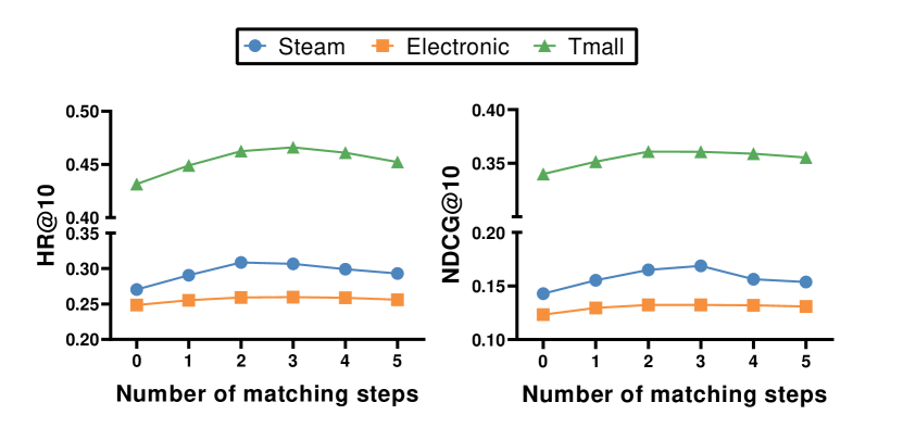
Figure 3: Performance w.r.t. the number of matching steps $t$.

Study of Mecos (RQ3)

Impact of matching steps. As the matching processor contributes a lot to Mecos, it is necessary to further study it. We consider changing the matching steps $t$ to study the influence of matching between query and reference. From Figure 3, increasing the number of matching steps significantly improves the model performance, which is contributed to the effective similarity matching of the recurrent matching processor. However, it is noteworthy that the performance of the model starts to decrease after we continue to increase matching steps. In general, the performance reaches its best when matching steps are maintained on two or three. The reason for that might be the overfitting due to too many steps. As the matching processor continuously injects information from the support set into the query representation in each matching step, the embedding space can become too crowded, resulting in the hubness problem. We can observe the clustering in the embedding visualization section (Figure 5).

Besides, by jointly comparing Table 2 and Figure 4, we observe that SR-GNN with Mecos is consistently superior to SR-GNN. Even without any matching steps, Mecos can also help the base model in alleviating the item cold-start problem. That again verifies the effectiveness and robustness of the framework.

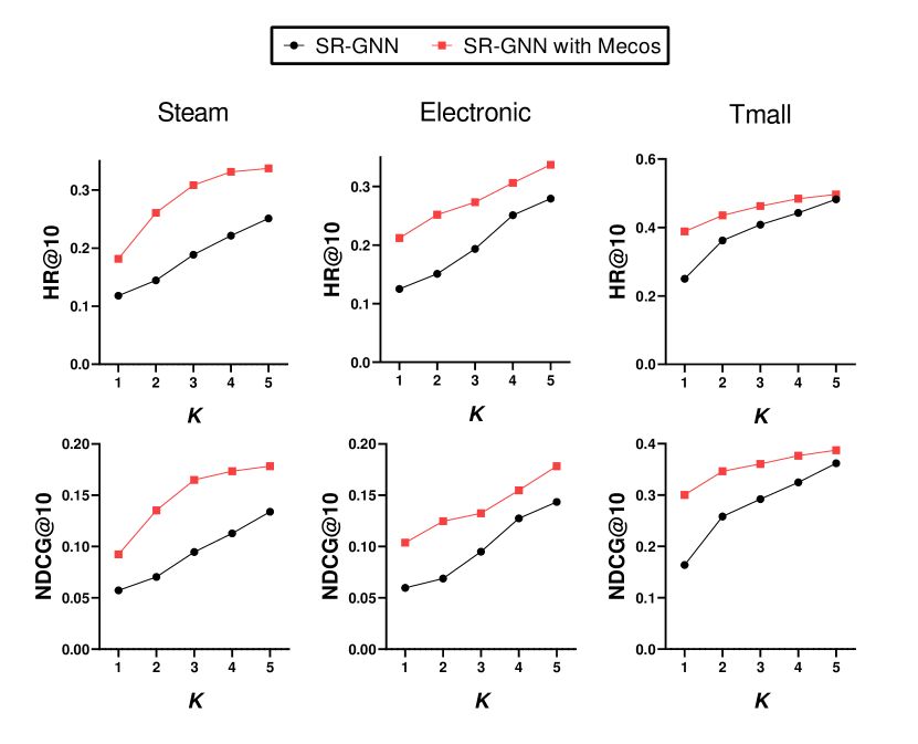
Figure 4: Performance w.r.t. the value of few-shot size $K$. The performance of SR-GNN with Mecos consistently outperforms SR-GNN.

Impact of support set size. Support set size $K$ represents how many instances that the model can use for training. To study the impact of it, we test Mecos with the strongest base model, SR-GNN, with different settings of $K$. According to Figure 4, performance increases with the increase of $K$. That is reasonable because a larger support set contains more known interactions for the target cold-start items. In this way, Mecos can provide a more precise characterization of the product’s potential users. And it is noteworthy that Mecos can also help a lot in cold-start item recommendation with only one-shot training instance ($K=1$), illustrating that Mecos produces reliable results even when training instances are extremely limited (e.g., one-shot learning).

However, for SR-GNN with Mecos, the growth trend of three metrics flattens out with the increase of the support set size $K$. And the performance gap between SR-GNN with and without Mecos is narrowing, indicating that Mecos is not suitable for items that have rich known interactions for training. That phenomenon is most obvious in Tmall datasets for it has the lowest proportion of cold-start items.

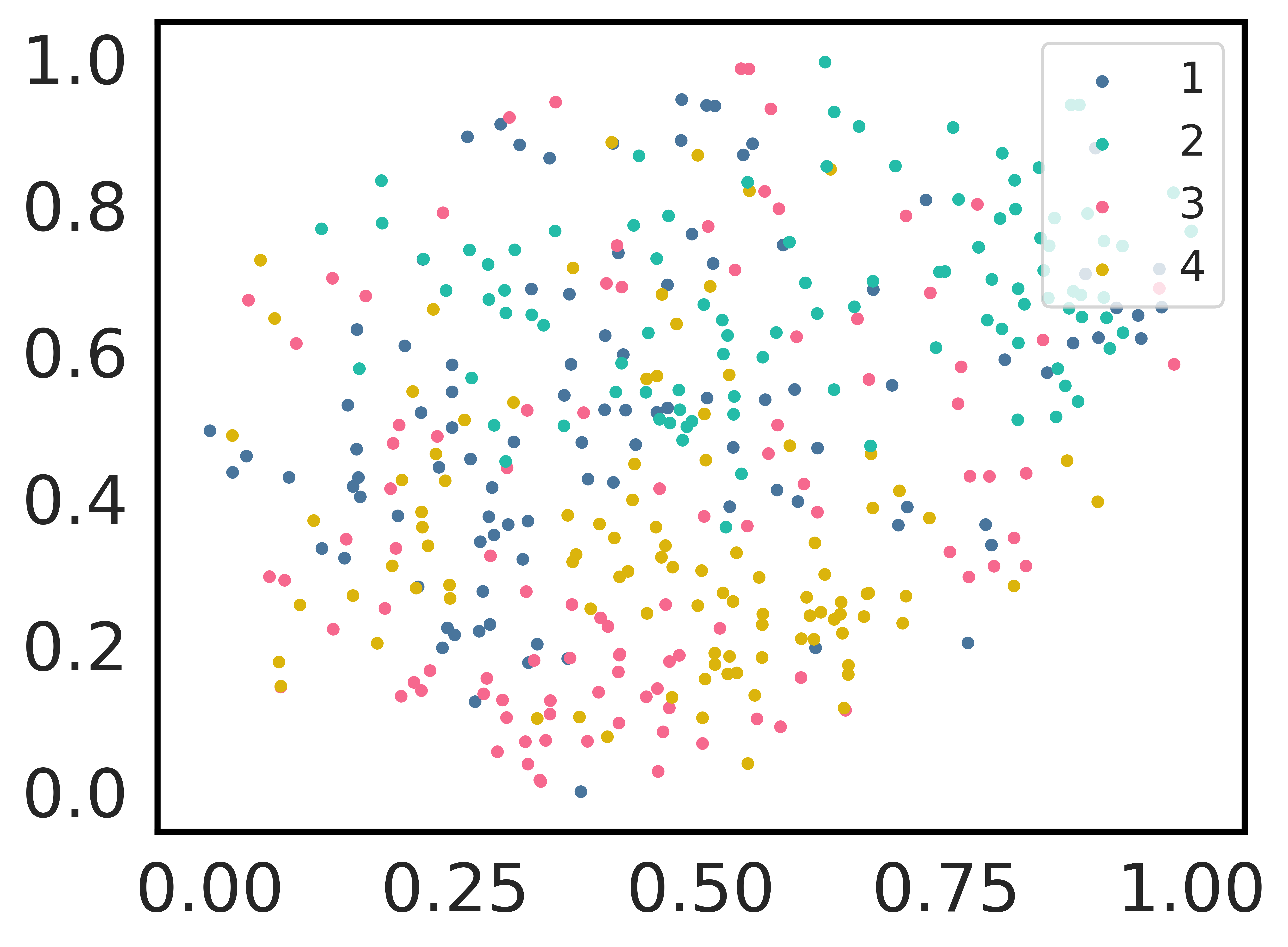
(a) SR-GNN

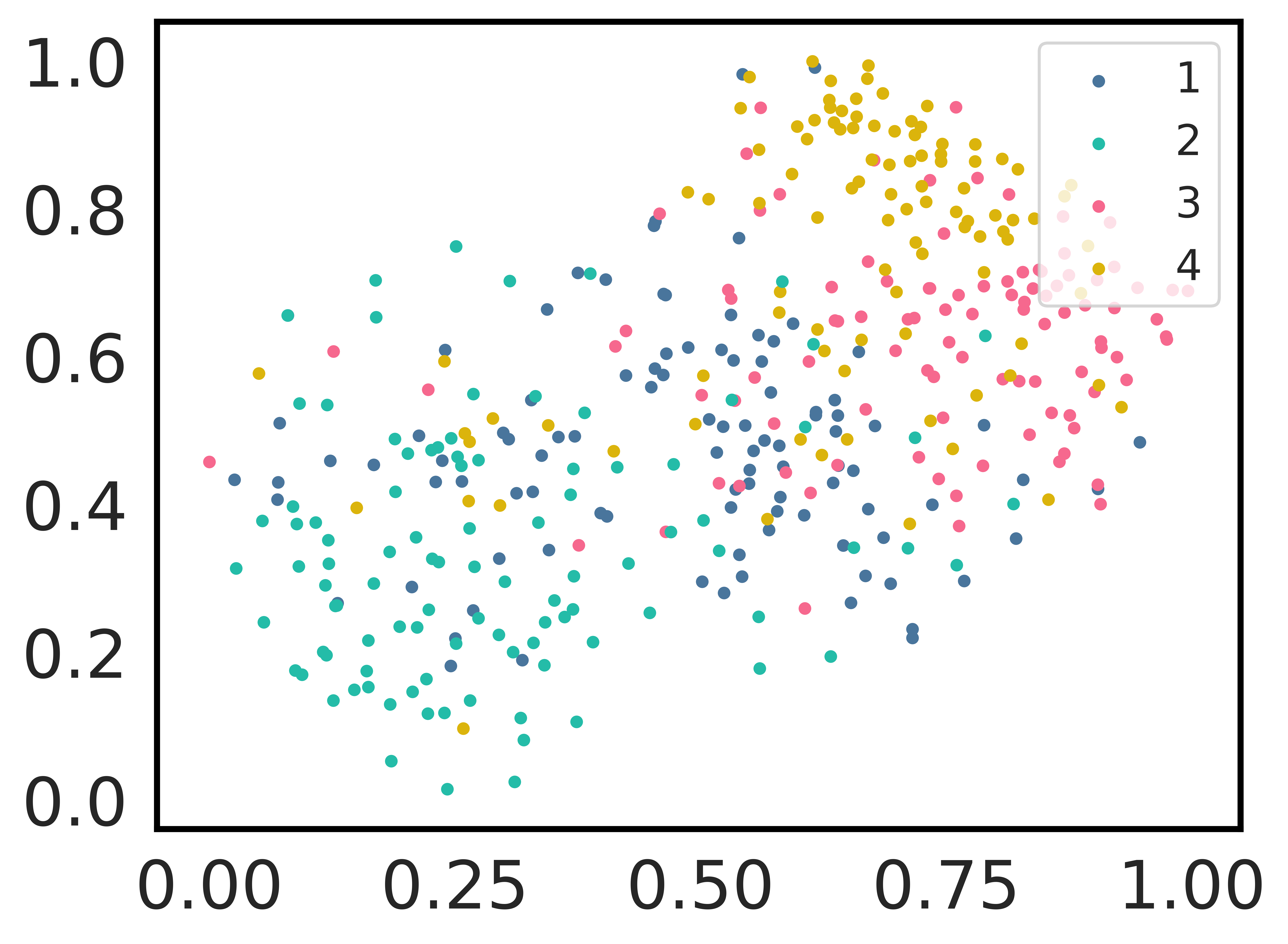
(b) SR-GNN with Mecos

Figure 5: Embedding visulization of query sequence pairs belonging to different candidate next-click items. Points with the same color denote sequence pairs belonging to the same target item.

Embedding Visualization (RQ4)

To intuitively study the impact of our framework, we visualize the query sequence pair embedding for different candidate next-click items by t-SNE (Hochreiter and Schmidhuber 2008). For each of those items, all others can be seen as negative data points. Thus, a reliable model should be able to distinguish these embeddings after training. We conduct the visualization on Steam with four different target items, each target item has 100 query sequence pairs. And we choose SR-GNN as the base model because it outperforms others in Steam. From Figure 5, it is clear that the model with Mecos better distinguishes different types of embeddings.

Conclusion

This work introduces Mecos to alleviate the item cold-start problem in sequential recommendation, which is an important problem in a novel and challenging context. With the pre-trained item embeddings as the input, our framework could be painlessly integrated with other state-of-the-art models. Mecos performs jointly optimization of the sequence pair encoder and the multi-step matching network. And a meta-learning based gradient descent approach is employed for parameter optimization. Once trained, our framework can be directly adapted to the new items updated in the online environment. Extensive experiments conducted on three real-world datasets illustrate the effect of Mecos and the contribution of each component.

References

- Barjasteh et al. (2016) Barjasteh, I.; Forsati, R.; Ross, D.; Esfahanian, A.-H.; and Radha, H. 2016. Cold-start recommendation with provable guarantees: A decoupled approach. TKDE 28(6): 1462–1474.
- Cui et al. (2018) Cui, Q.; Wu, S.; Liu, Q.; Zhong, W.; and Wang, L. 2018. MV-RNN: A multi-view recurrent neural network for sequential recommendation. IEEE Transactions on Knowledge and Data Engineering .
- Dong et al. (2020) Dong, M.; Yuan, F.; Yao, L.; Xu, X.; and Zhu, L. 2020. MAMO: Memory-Augmented Meta-Optimization for Cold-start Recommendation. In KDD.
- Du et al. (2019) Du, Z.; Wang, X.; Yang, H.; Zhou, J.; and Tang, J. 2019. Sequential Scenario-Specific Meta Learner for Online Recommendation. In KDD.
- Hidasi et al. (2015) Hidasi, B.; Karatzoglou, A.; Baltrunas, L.; and Tikk, D. 2015. Session-based recommendations with recurrent neural networks. In ICLR.
- Hochreiter and Schmidhuber (1997) Hochreiter, S.; and Schmidhuber, J. 1997. Long short-term memory. Neural computation 9(8): 1735–1780.
- Hochreiter and Schmidhuber (2008) Hochreiter, S.; and Schmidhuber, J. 2008. Visualizing data using t-SNE. Journal of machine learning research 9: 2579–2605.
- Hu, Zhang, and Yang (2018) Hu, G.; Zhang, Y.; and Yang, Q. 2018. Conet: Collaborative cross networks for cross-domain recommendation. In CIKM.
- Kang et al. (2019) Kang, S.; Hwang, J.; Lee, D.; and Yu, H. 2019. Semi-supervised learning for cross-domain recommendation to cold-start users. In CIKM.
- Kang and McAuley (2018) Kang, W.-C.; and McAuley, J. 2018. Self-attentive sequential recommendation. In ICDM.
- Lee et al. (2019) Lee, H.; Im, J.; Jang, S.; Cho, H.; and Chung, S. 2019. MeLU: Meta-Learned User Preference Estimator for Cold-Start Recommendation. In KDD.
- Li et al. (2019) Li, J.; Jing, M.; Lu, K.; Zhu, L.; Yang, Y.; and Huang, Z. 2019. From zero-shot learning to cold-start recommendation. In AAAI.
- Li et al. (2017) Li, J.; Ren, P.; Chen, Z.; Ren, Z.; Lian, T.; and Ma, J. 2017. Neural attentive session-based recommendation. In CIKM.
- Li et al. (2020) Li, X.; Zhang, M.; Wu, S.; Liu, Z.; Wang, L.; and Yu, P. S. 2020. Dynamic Graph Collaborative Filtering. In ICDM.
- Liu et al. (2018) Liu, Q.; Zeng, Y.; Mokhosi, R.; and Zhang, H. 2018. STAMP: short-term attention/memory priority model for session-based recommendation. In KDD.
- Liu and Zheng (2020) Liu, S.; and Zheng, Y. 2020. Long-tail Session-based Recommendation. In RecSys.
- McAuley et al. (2015) McAuley, J.; Targett, C.; Shi, Q.; and Van Den Hengel, A. 2015. Image-based recommendations on styles and substitutes. In SIGIR.
- Saveski and Mantrach (2014) Saveski, M.; and Mantrach, A. 2014. Item cold-start recommendations: learning local collective embeddings. In RecSys.
- Tan, Xu, and Liu (2016) Tan, Y. K.; Xu, X.; and Liu, Y. 2016. Improved recurrent neural networks for session-based recommendations. In DLRS.
- Tang and Wang (2018) Tang, J.; and Wang, K. 2018. Personalized top-n sequential recommendation via convolutional sequence embedding. In WSDM.
- Vartak et al. (2017) Vartak, M.; Thiagarajan, A.; Miranda, C.; Bratman, J.; and Larochelle, H. 2017. A meta-learning perspective on cold-start recommendations for items. In NIPS.
- Vinyals et al. (2016) Vinyals, O.; Blundell, C.; Lillicrap, T.; Wierstra, D.; et al. 2016. Matching networks for one shot learning. In NIPS.
- Wu et al. (2019) Wu, S.; Tang, Y.; Zhu, Y.; Wang, L.; Xie, X.; and Tan, T. 2019. Session-based recommendation with graph neural networks. In AAAI.
- Wu et al. (2020) Wu, S.; Yu, F.; Yu, X.; Liu, Q.; Wang, L.; Tan, T.; Shao, J.; and Huang, F. 2020. TFNet: Multi-Semantic Feature Interaction for CTR Prediction. In SIGIR.
- Yao et al. (2019) Yao, H.; Liu, Y.; Wei, Y.; Tang, X.; and Li, Z. 2019. Learning from multiple cities: A meta-learning approach for spatial-temporal prediction. In WWW.
- Yu et al. (2020) Yu, F.; Zhu, Y.; Liu, Q.; Wu, S.; Wang, L.; and Tan, T. 2020. TAGNN: Target Attentive Graph Neural Networks for Session-based Recommendation. In SIGIR.
- Zheng et al. (2020) Zheng, Y.; Liu, S.; Li, Z.; and Wu, S. 2020. DGTN: Dual-channel Graph Transition Network for Session-based Recommendation. In ICDMW.
- Zheng, Liu, and Zhou (2019) Zheng, Y.; Liu, S.; and Zhou, Z. 2019. Balancing Multi-level Interactions for Session-based Recommendation. arXiv preprint arXiv:1910.13527 .
- Zimdars, Chickering, and Meek (2001) Zimdars, A.; Chickering, D. M.; and Meek, C. 2001. Using temporal data for making recommendations. In UAI.