Beyond Class-Conditional Assumption: A Primary Attempt to Combat Instance-Dependent Label Noise

Abstract

Supervised learning under label noise has seen numerous advances recently, while existing theoretical findings and empirical results broadly build up on the class-conditional noise (CCN) assumption that the noise is independent of input features given the true label. In this work, we present a theoretical hypothesis testing and prove that noise in real-world dataset is unlikely to be CCN, which confirms that label noise should depend on the instance and justifies the urgent need to go beyond the CCN assumption.The theoretical results motivate us to study the more general and practical-relevant instance-dependent noise (IDN). To stimulate the development of theory and methodology on IDN, we formalize an algorithm to generate controllable IDN and present both theoretical and empirical evidence to show that IDN is semantically meaningful and challenging. As a primary attempt to combat IDN, we present a tiny algorithm termed self-evolution average label (SEAL), which not only stands out under IDN with various noise fractions, but also improves the generalization on real-world noise benchmark Clothing1M. Our code is released . Notably, our theoretical analysis in Section 2 provides rigorous motivations for studying IDN, which is an important topic that deserves more research attention in future.

1 Introduction

Noisy labels are unavoidable in practical applications, where instances are usually labeled by workers on crowdsourcing platforms (Yan et al. 2014; Schroff, Criminisi, and Zisserman 2010). Unfortunately, Deep Neural Networks (DNNs) can memorize noisy labels easily but generalize poorly on clean test data (Zhang et al. 2017). Hence, how to mitigate the effect of noisy labels in the training of DNNs has attracted considerable attention recently. Most existing works, for their theoretical analysis or noise synthesizing in experiments, follow the class-conditional noise (CCN) assumption (Scott, Blanchard, and Handy 2013; Zhang and Sabuncu 2018; Menon et al. 2020; Ma et al. 2020), where the label noise is independent of its input features conditional on the latent true label.

In fact, instances with the same label can be entirely different, hence the probability of mislabeling should be highly dependent on the specific instance. As shown in the first row of Fig. 1, the second right image is likely to be mislabeled as the number 6 and the fourth right image is likely to be manually mislabeled as the number 7; in the second row, the last image is more likely to be mislabeled as the ship. In this paper, our first contribution (Section 2) is to present a theoretical hypothesis testing on the well-known real-world dataset, Clothing1M, to demonstrate the urgent need to go beyond the CCN assumption in practical applications. Meanwhile, we discuss the challenge of instance-dependent noise (IDN) with both theoretical and empirical evidence. Some pioneer efforts has been contributed to IDN, but most results are restricted to binary classification (Menon, van Rooyen, and Natarajan 2018; Bootkrajang and Chaijaruwanich 2018; Cheng et al. 2020) or based on assumptions such as the noise is parts-dependent  (Xia et al. 2020).

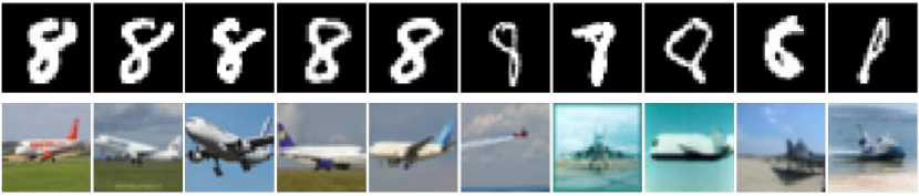
Figure 1: Examples of 8 in MNIST (first row) and Airplane in CIFAR-10 (second row). It is problematic to assume a same probability of mislabeling for diverse samples in each class.

To stimulate the development of theory and methodology on more practical-relevant IDN, we propose an algorithm to generate controllable IDN and present extensive characterizations of training under IDN, which is our second contribution (Section 3). Our third contribution (Section 4) is to propose an algorithm termed self-evolution average label (SEAL) to defend IDN, motivated by an experimental observation that the DNN’s output corresponding to the latent true label can be activated with oscillation before memorizing noise. Specifically, SEAL provides instance-dependent label correction by averaging predictions of a DNN on each instance over the whole training process, then retrains a classifier using the averaged soft labels. The superior performance of SEAL is verified on extensive experiments, including synthetic/real-world datasets under IDN of different noise fractions, and the large benchmark Clothing1M (Xiao et al. 2015) with real-world noise .

2 From CCN to IDN - Theoretical Evidence

2.1 Preliminaries

Considering a $c$-class classification problem, let $\mathcal{X}$ be the feature space, $\mathcal{Y}=\{1,...,c\}$ be the label space, $(X,Y)\in\mathcal{X}\times\mathcal{Y}$ be the random variables with distribution $\mathcal{D}_{X,Y}$ and $D=\{(x_{i},y_{i})\}_{i=1}^{n}$ be a dataset containing i.i.d. samples drawn from $\mathcal{D}_{X,Y}$. In practical applications, the true label $Y$ may not be observable. Instead, we have an observable distribution of noisy labels $(X,\bar{Y})\sim\mathcal{\bar{D}}_{X,\bar{Y}}$ and a dataset $\bar{D}=\{(x_{i},\bar{y}_{i})\}_{i=1}^{n}$ drawn from it. A classifier $f:\mathcal{X}\rightarrow\mathbb{P}^{c}$ is defined by a DNN that outputs a probability distribution over all classes, where $\mathbb{P}^{c}=\{s\in\mathbb{R}_{+}^{c}:\|s\|_{1}=1\}$. By default, the probability is obtained by a softmax function (Goodfellow, Bengio, and Courville 2016) at the output of $f$.

2.2 Beyond the CCN assumption

The CCN assumption is commonly used in previous works, as clearly stated in theoretical analysis (Blum and Mitchell 1998; Yan et al. 2017; Patrini et al. 2016; Zhang and Sabuncu 2018; Xu et al. 2019; Menon et al. 2020; Ma et al. 2020) or inexplicitly used in experiments for synthetizing noisy labels  (Han et al. 2018b; Yu et al. 2019; Arazo et al. 2019; Li, Socher, and Hoi 2020; Lukasik et al. 2020). Under the CCN assumption, the observed label $\bar{Y}$ is independent of $X$ conditioning on the latent true label $Y$.

Definition 1.

(CCN Model) Under the CCN assumption, there is a noise transition matrix $M\in[0,1]^{c\times c}$ and we observe samples $(X,\bar{Y})\sim\mathcal{\bar{D}}=\mathrm{CCN}(\mathcal{D},M)$, where first we draw $(X,Y)\sim\mathcal{D}$ as usual, then flip $Y$ to produce $\bar{Y}$ according to the conditional probability defined by $M$, i.e., $\mathrm{Pr}(\bar{Y}=q|Y=p)=M_{p,q}$, where $p,q\in\mathcal{Y}$.

We have seen various specific cases of CCN, including uniform/symmetric noise (Ren et al. 2018; Arazo et al. 2019; Chen et al. 2019a; Lukasik et al. 2020), pair/asymmetric noise (Han et al. 2018b; Chen et al. 2019b), tri/column/block-diagonal noise (Han et al. 2018a). Since the noise transition process is fully specified by a matrix $M$, one can mitigate the effect of CCN by modeling $M$ (Patrini et al. 2017; Hendrycks et al. 2018; Han et al. 2018a; Xia et al. 2019; Yao et al. 2019). Alternatively, several robust loss functions (Natarajan et al. 2013; Patrini et al. 2017; Zhang and Sabuncu 2018; Xu et al. 2019) have been proposed and justified. Many other works do not focus on theoretical analysis, yet propose methods based on empirical findings or intuitions, such as sample selection (Han et al. 2018b; Song, Kim, and Lee 2019; Yu et al. 2019), sample weighting (Ren et al. 2018) and label correction (Ma et al. 2018; Arazo et al. 2019).

Intuitively, it can be problematic to assign the same noise transition probability to diverse samples in a same class, which is illustrated by examples in Fig. 1. Theoretically, we can justify the need to go beyond the CCN assumption with the following theorem.

Theorem 1.

(CCN hypothesis testing) Given a noisy dataset with n instances, considering random sampling a validation set $\bar{D}^{\prime}=\{(x_{i},\bar{y}_{i})\}_{i=1}^{m},\,m<n$, and training a network $f$ on the rest instances. After training, the validation error on $\bar{D}^{\prime}$ is $\hat{er}_{\bar{D}^{\prime}}^{0-1}[f]=\sum_{i=1}^{m}\frac{1}{m}\mathbbm{1}(f(x_{i})\neq\bar{y}_{i})$, where $\mathbbm{1}(\cdot)$ is the indicator function. Let $w_{p}=\mathrm{Pr}[Y=p],\,p\in\mathcal{Y}$ be the fraction of samples in each class, then the following holds given the CCN assumption.

$$\mathrm{Pr}\left[1-\sum_{p=1}^{c}w_{p}\max_{q\in\mathcal{Y}}M_{p,q}-\hat{er}_{\bar{D}^{\prime}}^{0-1}[f]\geq\varepsilon\right]\leq e^{-2m\varepsilon^{2}}$$ (1)

Proof.

Let $er_{\mathcal{\bar{D}}}^{0-1}[f]=\mathbb{E}_{(X,\bar{Y})\sim\mathcal{\bar{D}}}\mathbbm{1}(f(X)\neq\bar{Y})$ be the generalization error on noisy distribution. For any $f$, the CCN assumption implies $f(X)$ is independent of $\bar{Y}$ conditional on $Y$, then we have,

$$er_{\mathcal{\bar{D}}}^{0-1}[f] =1-\mathbb{E}_{(X,\bar{Y})\sim\mathcal{\bar{D}}}\mathbbm{1}(f(X)=\bar{Y})$$

$$=1-\sum_{p=1}^{c}w_{p}\mathrm{Pr}[f(X)=\bar{Y}|Y=p]$$

$$=1-\sum_{p=1}^{c}w_{p}\sum_{q=1}^{c}\mathrm{Pr}[f(X)=q,\bar{Y}=q|Y=p]$$

$$=1-\sum_{p=1}^{c}w_{p}\sum_{q=1}^{c}\mathrm{Pr}[f(X)=q|Y=p]\cdot M_{p,q}$$

$$\geq 1-\sum_{p=1}^{c}w_{p}\max_{q\in\mathcal{Y}}M_{p,q}.$$

Note that the error $\hat{er}_{\bar{D}^{\prime}}^{0-1}[f]$ is estimated on validation samples that are not used when training $f$, hence $\mathbbm{1}(f(x_{i})\neq\bar{y}_{i}),i=1,\cdots,m$, are $m$ i.i.d Bernoulli random variables with expectation $er_{\mathcal{\bar{D}}}^{0-1}[f]$. Using Hoeffding’s inequality, we have, $\forall\varepsilon>0$,

$$\mathrm{Pr}\left[1-\sum_{p=1}^{c}w_{p}\max_{q\in\mathcal{Y}}M_{p,q}-\hat{er}_{\bar{D}^{\prime}}^{0-1}[f]\geq\varepsilon\right]$$

$$\leq\mathrm{Pr}\left[er_{\mathcal{\bar{D}}}^{0-1}[f]-\hat{er}_{\bar{D}^{\prime}}^{0-1}[f]\geq\varepsilon\right]\leq e^{-2m\varepsilon^{2}}.$$

∎

Now we apply Theorem 1 to the widely used noise benchmark Clothing1M, which contains $1M$ noisy training samples of clothing images in 14 classes. We train a ResNet-50 on $500K$ random sampled instances, validate on the rest and obtain a validation accuracy $\hat{er}_{\bar{D}^{\prime}}^{0-1}[f]=0.1605$. The original paper (Xiao et al. 2015) provides additional refined labels and a noise confusion matrix that can be an estimator of $M$ under the CCN assumption. Moreover, we estimate $w_{p}$ using the proportion of labels on the $14k$ refined subset. In this way, we get $1-\sum_{p=1}^{c}w_{p}\max_{q\in\mathcal{Y}}M_{p,q}=0.3817$. Now we have $1-\sum_{p=1}^{c}w_{p}\max_{q\in\mathcal{Y}}M_{p,q}-\hat{er}_{\bar{D}^{\prime}}^{0-1}[f]=0.2212$. By substituting $\varepsilon=0.2212$ to Eq. (1), we see that this result happens with probability lower than $\mathbf{10^{-21250}}$, which is statistically impossible. This contradiction implies that the CCN assumption does not hold on Clothing1M. In fact, this result is explainable by analyzing the difference between CCN and IDN. Under the CCN assumption, in each class, label noise is independent of input features, hence the network can not generalize well on such independent noise. Thus we derive a high validation error conditioning on CCN. While practically, we obtain an error much lower than the derived one, which implies that the network learned feature-dependent noise that can be generalized to the noisy validation set.

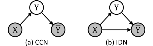
Figure 2: The graphical model of label noise.

2.3 The IDN model and its challenges

Now both theoretical evidence and the intuition imply that label noise should be dependent on input features, yet limited research efforts have been devoted to IDN. For binary classification under IDN, there have been several pioneer theoretical analysis on robustness (Menon, van Rooyen, and Natarajan 2018; Bootkrajang and Chaijaruwanich 2018) and sample selection methods (Cheng et al. 2020), mostly restricted to small-scale machine learning such as logistic regression. Under deep learning scenario, Xia et al. (2020) combat IDN by assuming that the noise is parts-dependent, hence they can estimate the noise transition for each part. Thulasidasan et al. (2019) investigate the co-occurrence of noisy labels with underlying features by adding synthetic features, such as the smudge, to mislabeled instances. However, this is not the typical realistic IDN where the noisy label should be dependent on inherent input features.

As presented in Definition 2, we can model instance-dependent mislabelling among given classes, where the noise transition matrix is a function of $X$. Note that both IDN and CCN consider close-set noise, as contrast to a specific label noise termed open-set noise (Wang et al. 2018), where the noisy instances does not belong to any considered classes. The graphical model of label noise is shown in Fig. 2. CCN can be seen as a degenerated case of IDN such that all instances have the same noise transition matrix.

Definition 2.

(IDN Model) Under the IDN model, $M:\mathcal{X}\rightarrow[0,1]^{c\times c}$ is a function of $X$. We observe samples $(X,\bar{Y})\sim\mathcal{\bar{D}}=\mathrm{IDN}(\mathcal{D},M)$, where first we draw $(X,Y)\sim\mathcal{D}$ as usual, then flip $Y$ to produce $\bar{Y}$ according to the conditional probability defined by $M(X)$ , i.e., $\mathrm{Pr}(\bar{Y}=q|Y=p)=M_{p,q}(X)$, where $p,q\in\mathcal{Y}$.

Many existing robust loss functions (Natarajan et al. 2013; Patrini et al. 2017; Zhang and Sabuncu 2018; Xu et al. 2019) have theoretical guarantees derived from the CCN assumption but not IDN. Some sample selection algorithms (Malach and Shalev-Shwartz 2017; Han et al. 2018b; Yu et al. 2019; Li, Socher, and Hoi 2020), targeting at selecting clean samples from the noisy training set, work quite well under CCN. Though these methods does not directly rely on the CCN assumption, it can be more challenging to identify clean samples under IDN since the label noise is correlated with inherent input features that result in confusion.

Theoretically, we show that the optimal sample selection exists under CCN but may fail under IDN. This is because under IDN, even if we select all clean samples, the distribution of $X$ can be different to its original distribution. While for CCN, we can select an optimal subset in theory. The key issue is whether the following holds for any $p\in\mathcal{Y}$.

$$supp(P(X|\bar{Y}=Y,Y=p))\overset{?}{=}supp(P(X|Y=p)),$$ (2)

where $supp(\cdot)$ is the support of a distribution. For CCN, since $X$ is independent of $\bar{Y}$ conditioning $Y$, the equality in Eq. (2) holds. While for IDN, it mostly does not hold. For example, if samples near the decision boundary are more likely to be mislabeled, then the support is misaligned for clean samples, which means learning with selected clean samples is statistically inconsistent (Cheng et al. 2020). More characterizations will be presented in the next section.

3 A typical controllable IDN

3.1 Enabling controllable experiments

The rapid advance of research on CCN not only attributes to simplicity of the noise model, but also the easy generation process of synthetic noise. We are able to conduct experiments on synthetic CCN with varying noise fractions by randomly flipping labels according to the conditional probability defined by $M$, which enable us to characterize DNNs trained with CCN (Arpit et al. 2017; Chen et al. 2019b), develop algorithms accordingly and quickly verify the idea. Similarly, it is desired to easily generate IDN with any noise fraction for any given benchmark dataset. A practical solution is to model IDN using DNNs’ prediction error because the error is expected to be challenging for DNNs. To yield calibrated softmax output for IDN generation, Berthon et al. (2020) train a classifier on a small subset, calibrate the classifier on another clean validation set (Guo et al. 2017), and then use predictions on the rest instances to obtain noisy labels. It does not generate noise for the whole dataset and the noise largely depends on the small training subset.

To stimulate the development of theory and methodology, we propose a novel IDN generator in Algorithm 1. Our labeler follows the intuition that ‘hard’ instances are more likely to be mislabeled (Du and Cai 2015; Menon, van Rooyen, and Natarajan 2018). Given a dataset $D=\{(x_{i},y_{i})\}_{i=1}^{n}$ with labels believed to be clean, we normally train a DNN for $T$ epochs and get a sequence of networks with various classification performance. For each instance, if many networks predict a high probability on a class different to the labeled one, it means that it is hard to clearly distinguish the instance from this class. Therefore, we can compute the score of mislabeling $N(x)$ and the potential noisy label $\tilde{y}(x)$ as follow:

$$\begin{split}S&=\sum_{t=1}^{T}S^{t}/T\in\mathbb{R}^{n\times c},\\ N(x_{i})&=\max_{k\neq y_{i}}S_{i,k},\quad\tilde{y}(x_{i})=\arg\max_{k\neq y_{i}}S_{i,k},\end{split}$$ (3)

where $S^{t}=[f^{t}(x_{i})]_{i=1}^{n}$ is DNN’s output at $t$-th epoch. The average prediction here reveals the DNN’s confusion on instances throughout training. We flip the label of $p\%$ instances with highest mislabeling scores, where $p$ is the targeted noise fraction. In essence, Algorithm 1 uses predictions of the DNN to synthetize noisy labels, while it stands out for being able to generate noisy labels of any noise ratio for the whole training set, requiring simply a single round of training on given labels. The noise is instance-dependent since it comes from the prediction error on each instance. Moreover, it is a typical challenging IDN since the error is exactly the class hard for the DNN to distinguish. In Appendix A, examples of noisy samples show that the noise is semantically meaningful.

Algorithm 1 IDN Generation.

  Input: Clean samples $D=\{(x_{i},y_{i})\}_{i=1}^{n}$, a targeted noise fraction $p$, epochs $T$.

  Initialize a network $f$.

  for $t=1$ to $T$ do

     for batches $\{(x_{i},y_{i})\}_{i\in\mathcal{B}}$ do

        Train $f$ on $\{(x_{i},y_{i})\}_{i\in\mathcal{B}}$ using cross-entropy loss: $\mathcal{L}_{CE}=-\frac{1}{\lvert\mathcal{B}\rvert}\sum_{i\in\mathcal{B}}\log(f_{y_{i}}^{t}(x_{i}))$

     end for

     Record output $S^{t}=[f^{t}(x_{i})]_{i=1}^{n}\in\mathbb{R}^{n\times c}$.

  end for

  Compute $N(x_{i})$, $\tilde{y}(x_{i})$ using $\{S^{t}\}_{t=1}^{T}$ (Eq. (3)).

  Compute the index set $\mathcal{I}=\{p\%\arg\max_{1\leq i\leq n}N(x_{i})\}$.

  Flip $\bar{y}_{i}=\tilde{y}_{i}$ if $i\in\mathcal{I}$ else keep $\bar{y}_{i}=y_{i}$.

  Output: A dataset with IDN: $\bar{D}=\{(x_{i},\bar{y}_{i})\}_{i=1}^{n}$.

3.2 Characterizations of training with IDN

To combat label noise, we can firstly characterize behaviors of DNNs trained with noise. For example, the memorization effect (Arpit et al. 2017) under CCN claims that DNNs tend to learn simple and general patterns first before memorizing noise, which has motivated extensive robust training algorithms. While our understanding on IDN is still limited. Here we present some empirical findings on IDN, to help researchers understand the behaviors of DNNs trained with IDN and to motivate robust training methods. We conduct experiments on MNIST and CIFAR-10 under IDN with varying noise fractions generated by Algorithm 1. For CCN, we use the most studied uniform noise. In all experiments throughout this paper, the DNN model and training hyperparameters we use are consistent. More details on experimental settings are summarized in Section 4.3 and Appendix B.

It is easier for DNNs to fit IDN.

Firstly, let us focus on the training/testing curves in Fig. 4. For IDN and CCN with the same noise fraction, the training accuracy is higher under IDN. This implies that it is easier for DNNs to fit IDN. The finding is consistent with our intuition since noisy labels under IDN are highly correlated with input features that can mislead DNNs. In this sense, IDN is more difficult to mitigate because the feature-dependent noise is very confusing for DNNs, which can easily result in overfitting. Moreover, the peak testing accuracy before convergence, which implies the DNN learns general patterns first (Arpit et al. 2017), is much lower under IDN. This suggests that due to DNNs can fit IDN easily, the generalization performance degenerates at early stages of training. The observation is consistent with the findings on real-world noise presented by Jiang et al. (2020).

The memorization effect is less significant.

The memorization effect (Arpit et al. 2017) is a critical phenomenon of DNNs trained with CCN: DNNs first learn simple and general patterns of the real data before fitting noise. It has motivated extensive robust training algorithms. The memorization effect is characterized by the testing accuracy and critical sample ratio (CSR) (Arpit et al. 2017) during training, where CSR estimates the density of decision boundaries. A sample $x$ is a critical sample if there exists a $\hat{x}$, s.t.,

$$\arg\max_{k}f_{k}(x)\neq\arg\max_{k}f_{k}(\hat{x}),\,\mathrm{s.t.}\,\|x-\hat{x}\|_{\infty}\leq r.$$ (4)

The curves of testing accuracy and CSR presented in Fig. 4 show typical characterizations of the memorization effect. Similar to CCN, the model achieves maximum testing accuracy before memorizing all training samples under IDN, which suggests that DNNs can learn general patterns first. Moreover, the CSR increases during training, suggesting that DNNs learn gradually more complex hypotheses. It is worth noting that under IDN, both peak testing accuracy and CSR are lower, and the gap between peak and converged testing accuracy is smaller. On MNIST, the testing accuracy decreases since very early stage of training, suggesting that the memorizing of noise dominates learning of real data. Therefore, we conclude that the memorization effect still exists under IDN, but it is less significant compared to CCN.

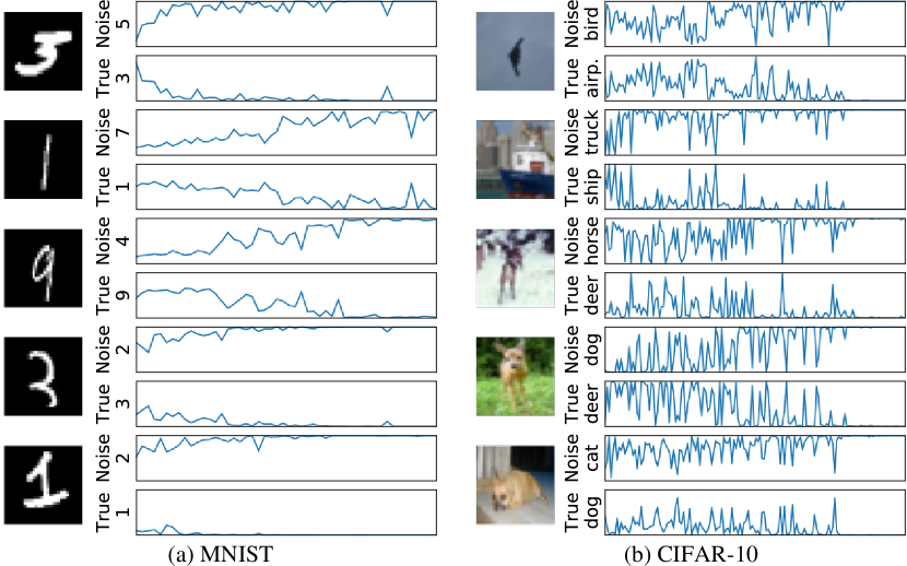
Figure 3: Examples of softmax outputs on the noisy label and latent true label. The x-axis is training epoch and the y-axis is DNN’s output probability. The airp. is airplane for short.

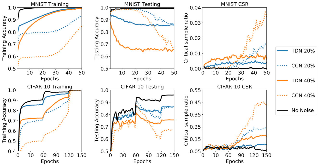
Figure 4: Training/testing accuracy and critical sample ratio throughout training on IDN and CCN with varying noise fractions.

Individual study: instance-level memorization.

Apart from showing the memorization effect for the whole training set, we are interested in how memorization happens for individual instances. As an individual study, we train DNNs under $20\%$ IDN and show examples in Fig. 3. We plot the entry of softmax output corresponding to the noisy label and true label throughout training. DNNs will eventually memorize the wrong label, while during training, the output corresponding to the true label can be largely activated with oscillation. The intensity of oscillation and the epoch when the memorization happens is quite different for each instance.

4 SEAL: a primary attempt to combat IDN

4.1 Methods

Algorithm 2 An iteration of SEAL.

  Input: Noisy samples $\bar{D}=\{(x_{i},\bar{y}_{i})\}_{i=1}^{n}$, epochs $T$, soft labels from the last iteration $\bar{S}$ (optional).

  Initialize a network $f$.

  if $\bar{S}$ is not available then

     $\#\,$The initial iteration, using one-hot noisy labels $\bar{S}=[e_{\bar{y}_{i}}]_{i=1}^{n}\in\mathbb{R}^{n\times c}$ where $e_{\bar{y}_{i}}$ is the one-hot label.

  end if

  for $t=1$ to $T$ do

     for batches $\{(x_{i},\bar{S}_{i})\}_{i\in\mathcal{B}}$ do

        Train $f$ on $\{(x_{i},\bar{S}_{i})\}_{i\in\mathcal{B}}$ using the loss:$\mathcal{L}_{SEAL}=-\frac{1}{\lvert\mathcal{B}\rvert}\sum_{i\in\mathcal{B}}\sum_{k=1}^{c}\bar{S}_{i,k}\log(f_{k}^{t}(x_{i}))$

     end for

     Record output $\bar{S}^{t}=[f^{t}(x_{i})]_{i=1}^{n}\in\mathbb{R}^{n\times c}$.

  end for

  Update $\bar{S}=\sum_{t=1}^{T}\bar{S}^{t}/T\in\mathbb{R}^{n\times c}$.

  Output: Trained $f$, $\bar{S}$ (can be used in next iteration).

To mitigate the effect of label noise, we propose a practical algorithm termed self-evolution average label (SEAL). SEAL provides instance-dependent label correction by averaging predictions of a DNN on each instance over the whole training process, then retrains a classifier using the averaged soft labels. An iteration of SEAL is outlined in Algorithm 2, and we can apply SEAL with multiple iterations.

Here we discuss the intuitions of SEAL. Without loss of generality, assume there exists a latent optimal distribution of true label for each instance. Let $S_{i}^{*}\in\mathbb{P}^{c}$ be the latent optimal label distribution of the $i$-th instance. $S_{i}^{*}$ can be one-hot for a confident instance and be soft otherwise. Intuitively, we can image $S_{i}^{*}$ as the output of an oracle DNN. Considering training a DNN on a $c$-class noisy dataset $\bar{D}=\{(x_{i},\bar{y}_{i})\}_{i=1}^{n}$ for sufficient many $T$ epochs until converged, we let $f^{t}(x_{i})$ be the output on $x_{i}$ at $t$-th epoch. Based on the oscillations show in Figure 3, we roughly approximate the output on $x_{i}$ at $t$-th epoch as

$$f^{t}(x_{i})=\alpha_{i}^{t}\omega_{i}^{t}+(1-\alpha_{i}^{t})e_{\bar{y}_{i}},$$ (5)

where $t\in\{1,2,\cdots,T\}$, $e_{\bar{y}_{i}}$ is the one-hot label, $\alpha_{i}^{t}\in[0,1]$ are coefficients dependent on instances and the network, $w_{i}^{t}\in\mathbb{P}^{c}$ are i.i.d. random vectors with $\mathbb{E}[w_{i}^{t}]=S_{i}^{*}$. The approximation may be inaccurate at the early stage of training because the network does not learn useful features and it is better to add a term for random predictions in the approximation. Still, we ignore this term because random predictions do not introduce bias toward any class and the effect is mitigated by taking the average. With the approximation, we intuitively compare with the prediction of a random epoch $f^{\tau}(x_{i})$, where $\tau$ is a random epoch such that $\mathrm{Pr}[\tau=t]=1/T,\forall t\in\{1,2,\cdots,T\}$. Let $\bar{S}\in\mathbb{R}^{n\times c}$ be the soft labels obtained by SEAL and $\|\cdot\|$ denote a norm on $\mathbb{P}^{c}$, it is not difficult to see that for any training instance $x_{i}$,

$$\|\mathbb{E}[\bar{S}_{i}]-S_{i}^{*}\|\leq\|e_{\bar{y}_{i}}-S_{i}^{*}\|,\\$$ (6)

$$\mathrm{var}(\bar{S}_{i,k})\leq\mathrm{var}(f_{k}^{\tau}(x_{i})),\,\forall k\in\{1,2,\cdots,c\}.$$ (7)

That is, SEAL yields instance-dependent label correction that is expected to be better than the given noisy labels and the label correction has lower variance due to taking the average.

We can run SEAL for multiple iteration to further correct the noise, and we term this ‘self-evolution’. We take the soft label (denoted as $\bar{S}_{i}^{[m]},m\geq 0$) of the last iteration as input and output $\bar{S}_{i}^{[m+1]}$. Using similar approximation as Eq. (5) by replacing the training label $e_{\bar{y}_{i}}$ with $\bar{S}_{i}^{[m]}$, SEAL is expected to produce labels that gradually approach the optimal ones,

$$\|\mathbb{E}[\bar{S}_{i}^{[m+1]}]-S_{i}^{*}\|\leq\|\bar{S}_{i}^{[m]}-S_{i}^{*}\|.$$ (8)

A concern of SEAL is the increased computational cost due to retraining the network. In experiments, we focus on verifying the idea of SEAL and we retrain networks from the scratch in each iteration to show the evolution under exactly the same training process, resulting in scaled computational cost. While in practice, we may save computational cost by reserving the best model (e.g., using a noisy validation set) and training for less epochs.

4.2 SEAL v.s. related methods

Using predictions of DNNs has long been adopted in distillation (Hinton, Vinyals, and Dean 2015) and robust training algorithms that use pseudo labels (Reed et al. 2015; Ma et al. 2018; Tanaka et al. 2018; Song, Kim, and Lee 2019; Nguyen et al. 2019; Arazo et al. 2019). SEAL provides an elegant solution that is simple, effective and has empirical and theoretical intuitions. Taking the average of predictions, motivated by the activation and oscillation of softmax output at the entry of true label, provides label correction. SEAL is different to vanilla distillation (Hinton, Vinyals, and Dean 2015): in the presence of label noise, simply distilling knowledge from a converged teacher network, which memorizes noisy labels, can not correct the noise.

Compared with existing pseudo-labeling methods, SEAL does not require carefully tuning hyperparameters to ensure that (i) the DNN learns enough useful features and (ii) the DNN dose not fit too much noise. It is challenging to compromise between (i) and (ii) in learning with IDN. We have shown that the memorization on correct/noisy labels can be quite different for each training instance. However, the above (i) and (ii) are typically required in existing methods (Reed et al. 2015; Ma et al. 2018; Tanaka et al. 2018; Song, Kim, and Lee 2019; Nguyen et al. 2019; Arazo et al. 2019). For example, one usually needs to tune a warm-up epoch (Tanaka et al. 2018; Song, Kim, and Lee 2019; Arazo et al. 2019) before which no label correction is applied. A small warm-up epoch results in underfitting on useful features while a large one yields overfitting on noise. Worse still, one may need to tune an adaptive weight during training to determine how much we trust predictions of the DNN (Reed et al. 2015; Ma et al. 2018). As theoretically shown by Dong et al. (2019), the conditions are very strict for DNNs to converge and not to fit noise.

When implementing SEAL, there is no specific hyperparameters other than the canonical hyperparameters such as the training epoch and learning rate. To determine these canonical hyperparameters, we simply need to examine the training accuracy on the noisy dataset. Since SEAL averages predictions throughout training, the label correction can be effective even if the DNN memorizes noise when converged. Therefore, our criterion of choosing hyperparameters is to make sure the training accuracy is converged and it is as high as possible. Moreover, the model architecture and training hyperparameters can be shared in each iteration of SEAL.

4.3 Empirical evaluation

Experimental setup.

Our experiments focus on challenging IDN and real-world noise. We demonstrate the performance of SEAL on MNIST and CIFAR-10 (Krizhevsky and Hinton 2009) with varying IDN fractions as well as large-scale real-world noise benchmark Clothing1M (Xiao et al. 2015). We use a CNN on MNIST and the Wide ResNet 28$\times$10 (Zagoruyko and Komodakis 2016) on CIFAR-10. On Clothing1M, we use the ResNet-50 (He et al. 2016) following the benchmark setting (Patrini et al. 2017; Tanaka et al. 2018; Xu et al. 2019). More details on experiments can be found in Appendix B.

SEAL corrects label noise.

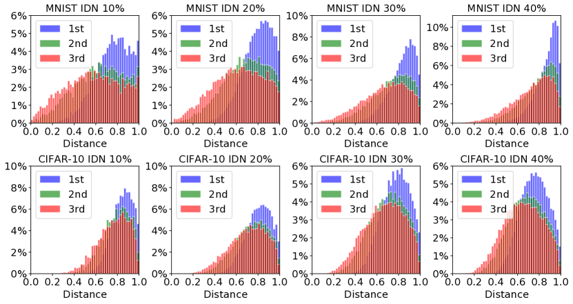
Figure 5: Histograms of distance distribution, where distance is evaluated between the true label and the soft label obtained by SEAL in 1-3 iteration.

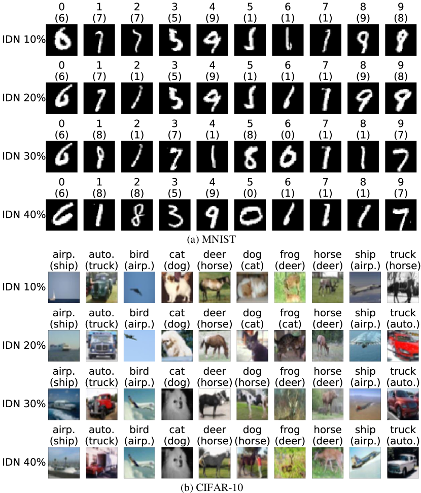
Figure 6: The noisy label and label correction (in parentheses) obtained from SEAL. The airp. and auto. are airplane and automobile for short.

We first evaluate distances between the true label and the soft label obtained by SEAL for all noisy instances. For each noisy instance, the distance is

$$d(\bar{S}_{i},y_{i})=\|\bar{S}_{i}-e_{y_{i}}\|_{1}/\|e_{\bar{y}_{i}}-e_{y_{i}}\|_{1}$$ (9)

where the denominator is to normalize the distance such that $d(\bar{S}_{i},y_{i})\in[0,1]$. Before running SEAL, the label is initialized as the one-hot observed label $e_{\bar{y}_{i}}$, hence the distance concentrates at 1.0. In Fig. 5, we show histograms of distance distribution for all noisy instances. When running SEAL iteratively, the distribution moves toward the left (distance reduced), suggesting that the updated soft label approaches the true label. This verifies that SEAL can correct label noise on varying datasets and noise fractions. To further investigate individual instances, we define $\bar{N}(x)$-the confidence that a label needs correction and $\tilde{y}(x)$-the label correction

$$\bar{N}(x_{i})=\max_{k\neq\bar{y}_{i}}\bar{S}_{i,k},\quad\tilde{y}(x_{i})=\arg\max_{k\neq\bar{y}_{i}}\bar{S}_{i,k}.$$ (10)

In Fig. 6, we present examples with the highest $\bar{N}(x)$ in each class, with the noisy observed label and proposed label correction (in parentheses) annotated on top of each image. SEAL can identify and correct noisy labels.

SEAL improves generalization under IDN.

Table 1: Classification accuracies ($\%$) on MNIST under instance-dependent label noise with different noise fractions.

Method	10$\%$	20$\%$	30$\%$	40$\%$
CE	94.07	85.62	75.75	65.83
	$\pm$0.29	$\pm$0.56	$\pm$0.09	$\pm$0.56
Forward	93.93	85.39	76.29	68.30
	$\pm$0.14	$\pm$0.92	$\pm$0.81	$\pm$0.42
Co-teaching	95.77	91.07	86.20	79.30
	$\pm$0.03	$\pm$0.19	$\pm$0.35	$\pm$0.84
GCE	94.56	86.71	78.32	69.78
	$\pm$0.31	$\pm$0.47	$\pm$0.43	$\pm$0.58
DAC	94.13	85.63	75.82	65.69
	$\pm$0.02	$\pm$0.56	$\pm$0.58	$\pm$0.78
DMI	94.21	87.02	76.19	67.65
	$\pm$0.12	$\pm$0.42	$\pm$0.64	$\pm$0.73
SEAL	96.75	93.63	88.52	80.73
	$\pm$0.08	$\pm$0.33	$\pm$0.15	$\pm$0.41

Table 2: Classification accuracies ($\%$) on CIFAR-10 under instance-dependent label noise with different noise fractions.

Method	10$\%$	20$\%$	30$\%$	40$\%$
CE	91.25	86.34	80.87	75.68
	$\pm$0.27	$\pm$0.11	$\pm$0.05	$\pm$0.29
Forward	91.06	86.35	78.87	71.12
	$\pm$0.02	$\pm$0.11	$\pm$2.66	$\pm$0.47
Co-teaching	91.22	87.28	84.33	78.72
	$\pm$0.25	$\pm$0.20	$\pm$0.17	$\pm$0.47
GCE	90.97	86.44	81.54	76.71
	$\pm$0.21	$\pm$0.23	$\pm$0.15	$\pm$0.39
DAC	90.94	86.16	80.88	74.80
	$\pm$0.09	$\pm$0.13	$\pm$0.46	$\pm$0.32
DMI	91.26	86.57	81.98	77.81
	$\pm$0.06	$\pm$0.16	$\pm$0.57	$\pm$0.85
SEAL	91.32	87.79	85.30	82.98
	$\pm$0.14	$\pm$0.09	$\pm$0.01	$\pm$0.05

We conduct experiments on MNIST and CIFAR-10 with IDN of varying noise fractions, compared with extensive baselines including (i) cross-entropy (CE) loss; (ii) Forward (Patrini et al. 2017), which trains a network to estimate an instance-independent noise transition matrix then corrects the loss; (iii) Co-teaching (Han et al. 2018b), where two classifiers select small-loss instances to train each other; (iv) Generalized Cross Entropy (GCE) loss, which is a robust version of CE loss with theoretical guarantee under CCN; (v) deep abstaining classifier (DAC) (Thulasidasan et al. 2019), which gives option to abstain samples depending on the cross-entropy error and an abstention penalty; (vi) Determinant based Mutual Information (DMI), which is an information-theoretic robust loss. The number of iterations is $10$ on MNIST and $3$ on CIFAR-10. SEAL consistently achieves the best generalization performance, as shown in Table 1 and Table 2, where we report the accuracy at the last epoch and repeat each experiment three times.

SEAL improves generalization under real-world noise.

Table 3: Testing accuracy ($\%$) on Clothing1M. The $*$ marks published results.

Method	Accuracy
CE$*$	68.94
Forward$*$	69.84
Co-teaching	70.15
GCE$*$	69.09
Joint Optimization$*$	72.16
DMI$*$	72.46
CE	69.07
SEAL	70.63
DMI	72.27
SEAL (DMI)	73.40

Clothing1M (Xiao et al. 2015) is a large-scale real-world dataset of clothes collected from shopping websites, with noisy labels assigned by the surrounding text. Following the benchmark setting (Patrini et al. 2017; Tanaka et al. 2018; Xu et al. 2019), the training set consists of $1M$ noisy instances and the additional validation, testing sets consist of $14K$, $10K$ clean instances. The number of SEAL iterations is $3$. In Table 3, we present the test accuracy. By default, SEAL is implemented with normal cross-entropy, where we see $1.56\%$ absolute improvement. Notably, SEAL also improves advanced training algorithms such as DMI (Xu et al. 2019) when we use the method as initialization.

5 Conclusion

In this paper, we theoretically justify the urgent need to go beyond the CCN assumption and study IDN. We formalize an algorithm to generate controllable IDN which is semantically meaningful and challenging. As a primary attempt to combat IDN, we propose a method SEAL, which is effective for both synthetic IDN and real-world noise.

Notably, our theoretical analysis in Section 2 provides rigorous motivations for studying IDN. Learning with IDN is an important topic that deserves more research attention in future.

6 Acknowledgments

The work is supported by the Key-Area Research and Development Program of Guangdong Province, China (2020B010165004) and the National Natural Science Foundation of China (Grant Nos.: 62006219, U1813204).

Appendix A Examples of noisy samples

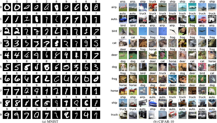
Figure 7: Our IDN labeler generates label noise (on top of each image) highly dependent on instances. As an example, each row corresponds to instances of the same true class, consisting of two correct instances and eight mislabeled instances. The airp. and auto. are airplane and automobile for short.

Appendix B More details on experiments

• On MNIST, we use a convolution neural network (CNN) with the standard input 28$\times$28 and 4 layers as follows: [conv 5$\times$5, filters 20, stride 1, relu, maxpool /2]; [conv 5$\times$5, filters 50, stride 1, relu, maxpool /2]; [fully connect 4*4*50$\rightarrow$500, relu]; [fully connect 500$\rightarrow$10, softmax]. Models are trained for 50 epochs with a batch size of 64 and we report the testing accuracy at the last epoch. For the optimizer, we use SGD with a momentum of 0.5, a learning rete of 0.01, without weight decay.

• On CIFAR-10, we use the Wide ResNet 28$\times$10. Models are trained for 150 epochs with a batch size of 128 and we report the testing accuracy at the last epoch. From Fig 4 in the main paper, we can see that the epoch of $150$ is sufficient large for the training accuracy to converges to $100\%$. For the optimizer, we use SGD with a momentum of 0.9 and a weight decay of $5\times 10^{-4}$ The learning rate is initialized as 0.1 and is divided by 5 after 60 and 120 epochs. We apply the standard data augmentation on CIFAR-10: horizontal random flip and 32$\times$32 random crop after padding 4 pixels around images. The standard normalization with mean=(0.4914, 0.4822, 0.4465), std=(0.2023, 0.1994, 0.2010) is applied before feeding images to the network.

• On Clothing1M, following the benchmark setting (Patrini et al. 2017; Tanaka et al. 2018; Xu et al. 2019), we use the ResNet-50 pre-trained on ImageNet and access the clean validation set consisting of $14K$ instances to do model selection. Models are trained for 10 epochs with a batch size of 256 on the noisy training set consisting of $1M$ instances. For the optimizer, we use SGD with a momentum of 0.9 and a weight decay of $10^{-3}$. We use a learning rate of $10^{-3}$ in the first 5 epochs and $10^{-4}$ in the second 5 epochs in all experiments except for DMI (Xu et al. 2019), where the learning rate is $10^{-6}$ and $0.5\times 10^{-6}$ according to its original paper. We apply the standard data augmentation: horizontal random flip and 224$\times$224 random crop. Before feeding images to the network, we normalize each image with mean and std from ImageNet, i.e., mean=(0.485, 0.456, 0.406), std=(0.229, 0.224, 0.225). Considering that a pre-trained model and a clean validation are accessed in all methods, we do not reinitialize our model in each SEAL iteration, instead, we start the training on top of the best model from the last iteration.

References

- Arazo et al. (2019) Arazo, E.; Ortego, D.; Albert, P.; O’Connor, N.; and Mcguinness, K. 2019. Unsupervised Label Noise Modeling and Loss Correction. In International Conference on Machine Learning.
- Arpit et al. (2017) Arpit, D.; Jastrzebski, S.; Ballas, N.; Krueger, D.; Bengio, E.; Kanwal, M. S.; Maharaj, T.; Fischer, A.; Courville, A.; Bengio, Y.; et al. 2017. A closer look at memorization in deep networks. In International Conference on Machine Learning.
- Berthon et al. (2020) Berthon, A.; Han, B.; Niu, G.; Liu, T.; and Sugiyama, M. 2020. Confidence Scores Make Instance-dependent Label-noise Learning Possible. arXiv preprint arXiv:2001.03772 .
- Blum and Mitchell (1998) Blum, A.; and Mitchell, T. 1998. Combining labeled and unlabeled data with co-training. In Proceedings of the eleventh annual conference on Computational learning theory.
- Bootkrajang and Chaijaruwanich (2018) Bootkrajang, J.; and Chaijaruwanich, J. 2018. Towards instance-dependent label noise-tolerant classification: a probabilistic approach. Pattern Analysis and Applications .
- Chen et al. (2019a) Chen, P.; Liao, B.; Chen, G.; and Zhang, S. 2019a. A meta approach to defend noisy labels by the manifold regularizer PSDR. arXiv preprint arXiv:1906.05509 .
- Chen et al. (2019b) Chen, P.; Liao, B. B.; Chen, G.; and Zhang, S. 2019b. Understanding and Utilizing Deep Neural Networks Trained with Noisy Labels. In International Conference on Machine Learning.
- Cheng et al. (2020) Cheng, J.; Liu, T.; Ramamohanarao, K.; and Tao, D. 2020. Learning with bounded instance-and label-dependent label noise. In International Conference on Machine Learning.
- Dong et al. (2019) Dong, B.; Hou, J.; Lu, Y.; and Zhang, Z. 2019. Distillation Early Stopping? Harvesting Dark Knowledge Utilizing Anisotropic Information Retrieval For Overparameterized Neural Network. arXiv preprint arXiv:1910.01255 .
- Du and Cai (2015) Du, J.; and Cai, Z. 2015. Modelling class noise with symmetric and asymmetric distributions. In AAAI Conference on Artificial Intelligence.
- Goodfellow, Bengio, and Courville (2016) Goodfellow, I.; Bengio, Y.; and Courville, A. 2016. Deep learning. MIT press.
- Guo et al. (2017) Guo, C.; Pleiss, G.; Sun, Y.; and Weinberger, K. Q. 2017. On calibration of modern neural networks. In International Conference on Machine Learning.
- Han et al. (2018a) Han, B.; Yao, J.; Niu, G.; Zhou, M.; Tsang, I.; Zhang, Y.; and Sugiyama, M. 2018a. Masking: A new perspective of noisy supervision. In Advances in Neural Information Processing Systems.
- Han et al. (2018b) Han, B.; Yao, Q.; Yu, X.; Niu, G.; Xu, M.; Hu, W.; Tsang, I.; and Sugiyama, M. 2018b. Co-teaching: Robust training of deep neural networks with extremely noisy labels. In Advances in Neural Information Processing Systems.
- He et al. (2016) He, K.; Zhang, X.; Ren, S.; and Sun, J. 2016. Deep residual learning for image recognition. In IEEE Conference on Computer Vision and Pattern Recognition.
- Hendrycks et al. (2018) Hendrycks, D.; Mazeika, M.; Wilson, D.; and Gimpel, K. 2018. Using trusted data to train deep networks on labels corrupted by severe noise. In Advances in Neural Information Processing Systems.
- Hinton, Vinyals, and Dean (2015) Hinton, G.; Vinyals, O.; and Dean, J. 2015. Distilling the knowledge in a neural network. arXiv preprint arXiv:1503.02531 .
- Jiang et al. (2020) Jiang, L.; Huang, D.; Liu, M.; and Yang, W. 2020. Beyond Synthetic Noise: Deep Learning on Controlled Noisy Labels. In International Conference on Machine Learning.
- Krizhevsky and Hinton (2009) Krizhevsky, A.; and Hinton, G. 2009. Learning multiple layers of features from tiny images. Technical report, Citeseer.
- Li, Socher, and Hoi (2020) Li, J.; Socher, R.; and Hoi, S. C. 2020. Dividemix: Learning with noisy labels as semi-supervised learning. In International Conference on Learning Representations.
- Lukasik et al. (2020) Lukasik, M.; Bhojanapalli, S.; Menon, A. K.; and Kumar, S. 2020. Does label smoothing mitigate label noise? In International Conference on Machine Learning.
- Ma et al. (2020) Ma, X.; Huang, H.; Wang, Y.; Romano, S.; Erfani, S.; and Bailey, J. 2020. Normalized Loss Functions for Deep Learning with Noisy Labels. In International Conference on Machine Learning.
- Ma et al. (2018) Ma, X.; Wang, Y.; Houle, M. E.; Zhou, S.; Erfani, S. M.; Xia, S.-T.; Wijewickrema, S.; and Bailey, J. 2018. Dimensionality-Driven Learning with Noisy Labels. In International Conference on Machine Learning.
- Malach and Shalev-Shwartz (2017) Malach, E.; and Shalev-Shwartz, S. 2017. Decoupling” when to update” from” how to update”. In Advances in Neural Information Processing Systems.
- Menon et al. (2020) Menon, A. K.; Rawat, A. S.; Reddi, S. J.; and Kumar, S. 2020. Can gradient clipping mitigate label noise? In International Conference on Learning Representations.
- Menon, van Rooyen, and Natarajan (2018) Menon, A. K.; van Rooyen, B.; and Natarajan, N. 2018. Learning from binary labels with instance-dependent noise. Machine Learning .
- Natarajan et al. (2013) Natarajan, N.; Dhillon, I. S.; Ravikumar, P. K.; and Tewari, A. 2013. Learning with noisy labels. In Advances in Neural Information Processing Systems.
- Nguyen et al. (2019) Nguyen, D. T.; Mummadi, C. K.; Ngo, T. P. N.; Nguyen, T. H. P.; Beggel, L.; and Brox, T. 2019. Self: Learning to filter noisy labels with self-ensembling. arXiv preprint arXiv:1910.01842 .
- Patrini et al. (2016) Patrini, G.; Nielsen, F.; Nock, R.; and Carioni, M. 2016. Loss factorization, weakly supervised learning and label noise robustness. In International Conference on Machine Learning.
- Patrini et al. (2017) Patrini, G.; Rozza, A.; Krishna Menon, A.; Nock, R.; and Qu, L. 2017. Making deep neural networks robust to label noise: A loss correction approach. In IEEE Conference on Computer Vision and Pattern Recognition.
- Reed et al. (2015) Reed, S. E.; Lee, H.; Anguelov, D.; Szegedy, C.; Erhan, D.; and Rabinovich, A. 2015. Training Deep Neural Networks on Noisy Labels with Bootstrapping. In International Conference on Learning Representations.
- Ren et al. (2018) Ren, M.; Zeng, W.; Yang, B.; and Urtasun, R. 2018. Learning to Reweight Examples for Robust Deep Learning. In International Conference on Machine Learning.
- Schroff, Criminisi, and Zisserman (2010) Schroff, F.; Criminisi, A.; and Zisserman, A. 2010. Harvesting image databases from the web. IEEE Transactions on Pattern Analysis and Machine Intelligence .
- Scott, Blanchard, and Handy (2013) Scott, C.; Blanchard, G.; and Handy, G. 2013. Classification with asymmetric label noise: Consistency and maximal denoising. In Conference on Learning Theory.
- Song, Kim, and Lee (2019) Song, H.; Kim, M.; and Lee, J.-G. 2019. SELFIE: Refurbishing Unclean Samples for Robust Deep Learning. In International Conference on Machine Learning.
- Tanaka et al. (2018) Tanaka, D.; Ikami, D.; Yamasaki, T.; and Aizawa, K. 2018. Joint optimization framework for learning with noisy labels. In IEEE Conference on Computer Vision and Pattern Recognition.
- Thulasidasan et al. (2019) Thulasidasan, S.; Bhattacharya, T.; Bilmes, J.; Chennupati, G.; and Mohd-Yusof, J. 2019. Combating Label Noise in Deep Learning using Abstention. In International Conference on Machine Learning.
- Wang et al. (2018) Wang, Y.; Liu, W.; Ma, X.; Bailey, J.; Zha, H.; Song, L.; and Xia, S.-T. 2018. Iterative learning with open-set noisy labels. In IEEE Conference on Computer Vision and Pattern Recognition.
- Xia et al. (2020) Xia, X.; Liu, T.; Han, B.; Wang, N.; Gong, M.; Liu, H.; Niu, G.; Tao, D.; and Sugiyama, M. 2020. Parts-dependent label noise: Towards instance-dependent label noise. In Advances in Neural Information Processing Systems.
- Xia et al. (2019) Xia, X.; Liu, T.; Wang, N.; Han, B.; Gong, C.; Niu, G.; and Sugiyama, M. 2019. Are Anchor Points Really Indispensable in Label-Noise Learning? In Advances in Neural Information Processing Systems.
- Xiao et al. (2015) Xiao, T.; Xia, T.; Yang, Y.; Huang, C.; and Wang, X. 2015. Learning from massive noisy labeled data for image classification. In IEEE Conference on Computer Vision and Pattern Recognition.
- Xu et al. (2019) Xu, Y.; Cao, P.; Kong, Y.; and Wang, Y. 2019. L_DMI: A Novel Information-theoretic Loss Function for Training Deep Nets Robust to Label Noise. In Advances in Neural Information Processing Systems.
- Yan et al. (2014) Yan, Y.; Rosales, R.; Fung, G.; Subramanian, R.; and Dy, J. 2014. Learning from multiple annotators with varying expertise. Machine learning .
- Yan et al. (2017) Yan, Y.; Xu, Z.; Tsang, I. W.; Long, G.; and Yang, Y. 2017. Robust semi-supervised learning through label aggregation. In AAAI Conference on Artificial Intelligence.
- Yao et al. (2019) Yao, J.; Zhang, Y.; Tsang, I. W.; and Sun, J. 2019. Safeguarded Dynamic Label Regression for Generalized Noisy Supervision. In AAAI Conference on Artificial Intelligence.
- Yu et al. (2019) Yu, X.; Han, B.; Yao, J.; Niu, G.; Tsang, I.; and Sugiyama, M. 2019. How does Disagreement Help Generalization against Label Corruption? In International Conference on Machine Learning.
- Zagoruyko and Komodakis (2016) Zagoruyko, S.; and Komodakis, N. 2016. Wide residual networks. arXiv preprint arXiv:1605.07146 .
- Zhang et al. (2017) Zhang, C.; Bengio, S.; Hardt, M.; Recht, B.; and Vinyals, O. 2017. Understanding deep learning requires rethinking generalization. In International Conference on Learning Representations.
- Zhang and Sabuncu (2018) Zhang, Z.; and Sabuncu, M. 2018. Generalized cross entropy loss for training deep neural networks with noisy labels. In Advances in Neural Information Processing Systems.